Robustness of discrete semifluxons in closed Bose-Hubbard chains

Abstract

We present the properties of the ground state and low-energy excitations of Bose-Hubbard chains with a geometry that varies from open to closed and with a tunable twisted link. In the vicinity of the symmetric $\pi-$flux case the system behaves as an interacting gas of discrete semifluxons for finite chains and interactions in the Josephson regime. The energy spectrum of the system is studied by direct diagonalization and by solving the corresponding Bogoliubov–de Gennes equations. The atom-atom interactions are found to enhance the presence of strongly correlated macroscopic superpositions of semifluxons.

1 Introduction

One-dimensional chains have attracted a great deal of interest in the past due to their simple analytical treatment both for bosons [1] and fermions [2]. The interplay between superfluidity and the effect of interactions in a one-dimensional system is particularly involved with some notable phenomena depending strongly on dimensionality, e.g. Tonks-Girardeau physics [3, 4]. Superfluid properties have been proved in dragged one-dimensional quantum fluids in open geometries [5], together with its breakdown due to interactions [6]. In closed periodic geometries, instead, condensate dragging can lead to a persistent current, experimentally observed in Refs. [7, 8, 9, 10]. Such persistent currents, which have already been experimentally produced in superconducting devices [11, 12, 13] as well as in polariton condensates [14], opened promising lines of research for future quantum computers [11]. In particular, states with half a quantum circulation or semifluxon states, have been detected in polariton spinor Bose-Einstein condensates [15], and have also been theoretically proposed in superconducting loops with Josephson junctions [16, 17].

The physics of persistent currents [9, 18] is intimately linked to phase slip events [19, 20], which have been widely discussed in (atomic [10, 9], superconductor [21, 22] and helium [23]) superfluids. They lead to the appearance of objects with topological defects (vortices, solitons) [24, 25] that can provoke counterflow superposition [25, 26]. Persistent currents may also be produced in ultracold atoms trapped in a few sites of an optical lattice [26, 27, 28, 29], such that one can profit from the nice properties of ultracold atomic experiments, namely the isolation from the environment and the control over the interactions and geometry [30, 31]. In this way we have previously shown how topological defects can be produced by manipulating the phase-dependence of a single link [32]. There, a key ingredient was added to the Bose-Hubbard trimer: a single tunable tunnelling link between two modes. This tunable hopping rate can be eventually turned to negative, which in the symmetric configuration induces a $\pi$ flux through the trimer, thus producing a two-fold degeneracy in the ground state of the single-particle spectrum. These two-fold degenerate states can be interpreted as discrete semifluxon states and provide the basis for the description of the ground state of the system, which is, under certain conditions, a cat state of semifluxon-antisemifluxon states. This symmetric $\pi-$flux case is gauge equivalent to a rotating trimer with a $\pi/3$ phase change between all sites, a configuration which has received attention in the past [33]. It is also gauge equivalent to the melting of vortex states studied in a higher part of the spectrum in Ref. [34]. Our symmetric configuration provides a specific gauge, which implies a feasible experimental way of producing superpositions of semifluxon states.

In this article, we generalize our earlier studies of three-site configurations to general closed Bose-Hubbard chains with any number of sites. Forcing one of the links to flip the quantum phase, macroscopic superpositions of discrete semifluxon states are found to form the degenerate set of ground states of the system for small but finite atom-atom interactions. This feature makes this setup particularly appealing in contrast to the fully symmetric chains considered before [27], where persistent currents in closed Bose-Hubbard configurations were studied for excited states. There are nowadays a variety of experimental setups capable to simulate such chains, e.g. ultracold atomic gases trapped in a circular array [35]. Beyond ultracold atomic systems, Bose-Hubbard Hamiltonians have recently been engineered in experiments with coupled non-linear optical resonators [36], where a two-mode Bose-Hubbard dimer has been produced with all relevant parameters externally controlled. The extension of these setups to three or more modes is a promising open line of research. Exciton polaritons provide another experimental root to engineer these Hamiltonians, since soon after the two-modes case [37] discrete ring optical condensates have also been reported [38].

Our setup demands a good control on the tunnelling rate between two sites of a Bose-Hubbard chain, both in strength and phase. Ultracold atomic gases have provided several proposals to achieve such dependence of the tunnelling terms in the case of external modes [39, 40, 41]. Another option would be to replace the external sites for internal ones, building the connected Bose-Hubbard chain of internal atomic sublevels. In this case, the real one dimensional system is replaced by an extra dimension built from the internal sublevels, in the language of Ref. [42]. In this case a phase-dependent tunnelling can be obtained through the Jaksch-Zoller mechanism [43].

The paper is organized as follows. Section 2 introduces the Hamiltonian that describes the Bose-Hubbard chain with a tunable tunnelling. In Sect. 3, we will analyze in detail the properties of the single-particle problem. Section 4 is devoted to study the coherent ground state of the system and excitations over mean-field states. In Sect. 5 we present the macroscopic superposition of semifluxon states that appears for a given set of parameters, and we investigate their robustness in Sect. 6. We summarize our results and provide future perspectives in Sect. 7.

2 Tunable Bose-Hubbard Hamiltonian

We consider $N$ ultracold interacting bosons populating $M$ quantum states (sites). Following standard procedures [31] the system is described in the lower-band approximation by the Bose-Hubbard (BH) Hamiltonian $\hat{\cal H}=\hat{\cal T}+\hat{\cal U}$, which, under the notation of Ref. [27] takes the form:

$$\hat{\cal T} = -\gamma J\,(\hat{a}^{{\dagger}}(M)\,\hat{a}(1)+{\rm h.c.})-J\sum_{\lambda=1}^{M-1}\left(\hat{a}^{{\dagger}}(\lambda)\,\hat{a}(\lambda+1)+{\rm h.c.}\right)$$

$$\hat{\cal U} = \frac{U}{2}\sum_{\lambda=1}^{M}\hat{a}^{{\dagger}}(\lambda)\,\hat{a}^{{\dagger}}(\lambda)\,\hat{a}(\lambda)\,\hat{a}(\lambda)\,,$$ (1)

where $\hat{a}(\lambda)$ ($\hat{a}^{\dagger}(\lambda)$) are the bosonic annihilation (creation) operators for site $\lambda$, fulfilling canonical commutation relations. $J$ is the tunnelling amplitude between consecutive sites and the parameter $U$ takes into account the on-site atom-atom interaction, which is proportional to the $s$-wave scattering length and is assumed to be repulsive, $U>0$. Attractive atom-atom interactions can also be produced and would more naturally lead to macroscopic superposition states but they are fragile against instabilities. We will analyse the ground state structure and the excitation spectrum as a function of the dimensionless parameter $\Lambda\equiv NU/J$, which gives the ratio between interaction and tunnelling rate.

As mentioned in the introduction, a crucial ingredient in our model is the presence of a single tunable link. In practice, the tunnelling between sites $1$ and $M$ can be varied through a parameter $\gamma$, which is taken to be real. This allows to study very different configurations, for instance, an open 1D Bose-Hubbard chain when $\gamma=0$, and a symmetric non-twisted (twisted) closed chain when $\gamma=1(\gamma=-1)$. In the latter two cases $\hat{\cal H}$ is particularly simple. It can be shown that, for the special cases $\gamma=\pm 1$, $\hat{\cal H}$ is gauge equivalent to a symmetric Hamiltonian (equal couplings) with a total flux $\Phi=0$ and $\Phi=\pi$, respectively:

$$\hat{\cal H}_{\rm sym}=-J\sum_{\lambda=1}^{M}\ \left[e^{i\Phi/M}\,\hat{a}^{\dagger}(\lambda)\,\hat{a}(\lambda+1)+{\rm h.c.}\right]+\hat{\cal U}\,.$$ (2)

In the previous equation, the site $\lambda=M+1$ corresponds to site $1$ (periodicity of the chain). This many-body Hamiltonian describes a Bose-Hubbard 1D circular chain, rotating around its symmetry axis with angular frequency $\Phi$ [33, 27, 44]. Therefore, the physics of the special $\gamma=\pm 1$ cases will be essentially equivalent to the ones considered prior. However, it is worth emphasizing that such local gauge transformation relating the Hamiltonians in Eq. (1) and Eq. (2) does not exist for a general value of $\gamma$.

3 The non-interacting problem

3.1 Single-particle problem

For a single particle the problem reduces to finding the eigenvalues $\mu$ and eigenvectors $\chi(\lambda)$, with $\lambda=1,\dots,M$, of $\hat{\cal T}$:

$$\left(\matrix{\mu&J&0&\cdots&0&0&\gamma J\cr J&\mu&J&\cdots&0&0&0\cr 0&J&\mu&\cdots&0&0&0\cr\vdots&\vdots&\vdots&\ddots&\vdots&\vdots&\vdots\cr 0&0&0&\cdots&\mu&J&0\cr 0&0&0&\cdots&J&\mu&J\cr\gamma J&0&0&\cdots&0&J&\mu}\right)\left(\matrix{\chi(1)\cr\chi(2)\cr\chi(3)\cr\vdots\cr\chi(M-2)\cr\chi(M-1)\cr\chi(M)}\right)=0\ .$$ (3)

Using standard techniques in solving tight binding problems, one finds that the solutions can be either even (symmetric): $\chi^{(S)}(\lambda)=\chi^{(S)}(M+1-\lambda)$ or odd (antisymmetric): $\chi^{(A)}(\lambda)=-\chi^{(A)}(M+1-\lambda)$. They can be written conveniently in terms of Bloch phases $\phi$ as

$$\chi^{(S)}(\lambda) = \frac{1}{\sqrt{\cal{N}_{+}}}\ \cos\left[\left(\frac{M+1}{2}-\lambda\right)\phi\right]\,,$$

$$\chi^{(A)}(\lambda) = \frac{1}{\sqrt{\cal{N}_{-}}}\ \sin\left[\left(\frac{M+1}{2}-\lambda\right)\phi\right]\,,$$ (4)

where the normalization factor of each wave function is ${\cal N}_{\pm}=(M\pm\sin(M\phi)/\sin\phi)/2$. The respective Bloch phases satisfy the implicit equations,

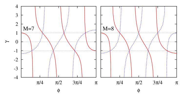
Figure 1: Graphical real solutions of Eq. (5), even solutions, solid red lines, and Eq. (6), odd solutions, dashed blue lines. As en example we depict horizontal lines for $\gamma=\pm 1$, dotted black lines. For a given $\gamma$, the solutions correspond to the crossings between the horizontal dotted line and the solid and dashed lines. The number of sites considered is $M=7$ (left) and $M=8$ (right).

$$\gamma=\frac{\cos(\phi(M+1)/2)}{\cos(\phi(M-1)/2)}$$ (5)

for the even solutions, and

$$\gamma=-\frac{\sin(\phi(M+1)/2)}{\sin(\phi(M-1)/2)}$$ (6)

for the odd ones. In terms of the Bloch phases, the eigenvalues ($\mu$) are then given by

$$\mu=-2J\cos\phi\ .$$ (7)

Figure 1 shows the right hand side of the Eqs. (5) and  (6) for symmetric (solid red) and antisymmetric (dashed blue) wave functions for a chain with $M=7$ and $M=8$. Drawing a horizontal line at the chosen value of $\gamma$, the crossings determine graphically the solutions for real $\phi$, as illustrated for the cases $\gamma=1$ and $-1$. Notice the odd/even degeneracies that appear for $\gamma=\pm 1$, a characteristic feature of these two cases, and their absence for any other values of $\gamma$. It can be checked that the $\gamma=+1$ solutions are $\phi_{q}=2\pi q/M$, with $q=0,\dots,M-1$, all twice degenerate except the first. Similarly, when $\gamma=-1$ the solutions are $\phi_{q}=\frac{2\pi}{M}(q+\frac{1}{2})$, with $q=0,\dots,M-1$, all twice degenerate except the last.

For arbitrary $\gamma$, all the real solutions that can be extracted from those figures fulfill the condition $0\leq\phi\leq\pi$. Therefore the corresponding energies, Eq. (7), are in the band $-2J\leq\mu\leq 2J$, and the associated eigenstates are “bulk states”, see discussion in Sect. 6. This is in agreement with the results in Fig. 2, which shows the single-particle spectrum as a function of $\gamma$ for $M=3,4,5$ and $6$. However, there are some special states whose energy is not contained within the previous interval. They correspond to “surface states”, and will be discussed later.

The poles of Fig. 1 (which give the solutions when $|\gamma|\to\infty$) are determined by the zeros of the denominators in Eqs. (5) and (6), i.e. $\phi^{(S,A)}_{k,(|\gamma|\to\infty)}=\pi k/(M-1)$ where $k$ accounts for the odd (even, including $k=0$) natural numbers for the symmetric (antisymmetric) wave function. As seen in Fig. 1 each $\phi$ corresponding to a finite $\gamma$ is bounded by those of two consecutive poles $\phi_{k-1,(|\gamma|\to\infty)}^{(S,A)}\ <\ \phi^{(S,A)}_{k}\ <\ \phi_{k,(|\gamma|\to\infty)}^{(S,A)}$, where $\phi_{-1,(|\gamma|\to\infty)}$ has to be taken as $0$. These inequalities show that there are no crossings of single-particle levels of the same parity. This feature can be readily seen in Fig. 2, since even single-particle levels (filled symbols) do not intersect levels corresponding to other even-parity states, independently of the number of sites (and the same occurs for odd-parity states, represented by open symbols). Note also that the curves associated to the solid red (dashed blue) lines in Fig. 1 are monotonically decreasing (increasing). Thus a monotonic variation of $\gamma$ gives also a monotonic variation of its corresponding energy in Fig. 2.

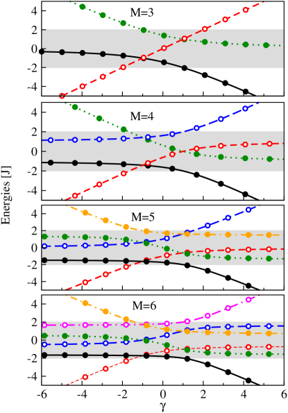
Figure 2: Single-particle spectrum for the cases $M=3$, $4$, $5$ and $6$ sites, as a function of $\gamma$. Filled (open) symbols characterize levels with even (odd)-parity states. The grey region encompasses the range of eigenvalues $|\mu|<2J$, which contains all the states with real Bloch phase, bulk states. The states outside this region, which have imaginary Bloch phase (see the text), are surface states. Energies are in units of $J$.

3.2 Extension to imaginary values of $\phi$: Surface states.

The remaining (up to $M$) eigenstates of Eq. (3) correspond to surface states and require imaginary values of the Bloch phase: $\phi=i\eta$, with $\eta$ real. Then the implicit equation for the eigenvalues (5), becomes

$$\gamma=\frac{\cosh(\eta(M+1)/2)}{\cosh(\eta(M-1)/2)}\,.$$ (8)

and at small $\eta$, the r.h.s. behaves as $1+M/2\ \eta^{2}$ and leads therefore to $\gamma>1$. For large $\eta$ the r.h.s. rises as $e^{\eta}$ and guarantees that there will be solutions for any $\gamma>1$.

For the antisymmetric solutions one has to introduce also $\phi=i\eta$ and the r.h.s of Eq. (6) becomes

$$\gamma=-\frac{\sinh(\eta(M+1)/2)}{\sinh(\eta(M-1)/2)}$$ (9)

and for small $\eta$

$$\gamma\simeq-\frac{M+1}{M-1}\left(1+\frac{1}{6}M\eta^{2}\right)<-{M+1\over M-1}$$ (10)

in agreement with the lower bound in Fig. 1. The asymptotic behaviour for large $\eta$ is now $\gamma\simeq-$ exp$(\eta)$.

Figure 1 also shows that there is a similar problem with the solutions associated to states with highest $\phi$, corresponding to the surface states above the grey region in Fig. 2. In this case one has to set $\phi=\pi+i\eta$ to find the missing solution.

In analogy to the expression of $\gamma$ as a function of the imaginary Bloch phase, the eigenenergies change as well, $\mu=-2J\cosh\eta$, which at large values of $\eta$ becomes $\mu=\mp 2J\gamma$, for the even ($-$) and odd ($+$) surface states. This explains the asymptotic linear behaviour of the energies of these states shown in Fig. 2.

3.3 The special $\gamma=\pm 1$ cases

Fig. 2 shows that the cases of $\gamma=\pm 1$ exhibit degeneracy points where the eigenvectors are linear combinations of the solutions of the previous Hamiltonian. Remarkably, these new states are no longer currentless. One can construct a basis of flow states (from now on, “flow basis”), which can be obtained from the bare states through a unitary transformation,

$${\tilde{\chi}}_{q}(\lambda;\gamma=+1) = \frac{1}{\sqrt{M}}e^{i\frac{2\pi}{M}q\lambda}$$

$${\tilde{\chi}}_{q}(\lambda;\gamma=-1) = \frac{1}{\sqrt{M}}e^{i\frac{2\pi}{M}(q+1/2)\lambda}\ .$$ (11)

These expressions imply equidistributed particle population within all the sites but with a phase variation whose gradient between sites lead to an azimutal velocity.

The $\gamma=1$ case is the commonly considered situation in the literature, as it also appears in the usual tight-binding models in condensed matter systems. Concerning the currents, there is one important difference between $\gamma=1$ and $\gamma=-1$. In the former case, the ground state of the system corresponds to $\phi=0$, which is a currentless state. It is always non-degenerate and its eigenenergy is $\mu_{gs}=-2J$, independently of the number of sites $M$. The first two excited states are degenerate and correspond to $\phi=2\pi/M$ and $-2\pi/M$. They are the discrete version of the usual vortex states (also called fluxons) with a circulation of $\pm 2\pi$ [34, 27]. In contrast, the ground state of a BH closed chain with $\gamma=-1$ is always degenerate. It is spanned by the eigenvectors corresponding to $q=0\,(\phi=\pi/M)$ and $q=M-1\,(\phi=-\pi/M)$ in Eq. (11), which are discrete semifluxon/antisemifluxon states (half-vortices with $\pm\pi$ circulation, see Appendix A for further discussion of their properties). The energy gap $\Delta\equiv\mu_{\rm ex}-\mu_{\rm gs}$ between the degenerate ground states and the first excitation is

$$\Delta=4J\sin(\pi/M)\,\sin(2\pi/M)\simeq 8{J\pi^{2}/M^{2}}\,.$$ (12)

As explained above, the $\gamma=-1$ case can be related by a local gauge transformation to a BH Hamiltonian in which each hopping induces a $\pi/M$ phase, as in Eq. (2). In that case, considered for instance in Ref. [33] for $M=3$, the degeneracy takes place between the fully symmetric ground state for $\gamma=1$, and one of the vortex states.

4 Many-body coherent states

The eigensolutions of $\hat{\cal T}$ described in the previous Section define a new basis for the single particle states, the “mode” basis. The associated creation and annihilation operators will be written as $\hat{b}_{q}^{{\dagger}}$ and $\hat{b}_{q}$, $q=1,\dots,M$, so that

$$\hat{b}_{q}^{{\dagger}} = \sum_{\lambda}\chi_{q}(\lambda)\,\hat{a}^{{\dagger}}(\lambda)\,,\quad\hat{b}_{q}=\sum_{\lambda}\chi^{*}_{q}(\lambda)\,\hat{a}(\lambda)\ ,$$ (13)

with all sums running from $1$ to $M$. From unitarity we have

$$\sum_{\lambda}\chi_{q}^{*}(\lambda)\chi_{q^{\prime}}(\lambda)=\delta_{qq^{\prime}}\,,\quad\sum_{q}\chi_{q}^{*}(\lambda^{\prime})\ \chi_{q}(\lambda)=\delta_{\lambda\lambda^{\prime}}\ ,$$ (14)

and thus $[\hat{b}_{q},\hat{b}^{{\dagger}}_{p}]=\delta_{qp}$. And also that $\hat{a}^{{\dagger}}(\lambda)=\sum_{q}\chi^{*}_{q}(\lambda)\ \hat{b}^{{\dagger}}_{q}$ and $\hat{a}(\lambda)=\sum_{q}\ \chi_{q}(\lambda)\ \hat{b}_{q}\,.$

The coherent states, defined as

$$|\Psi_{q}^{(N)}\rangle \equiv \frac{1}{\sqrt{N!}}(\hat{b}_{q}^{\dagger})^{N}|{\rm vac}\rangle=|0,0,...,N,..0\rangle$$

(15)

will be also named mean-field states for $N$ bosons. For the special cases when $\gamma=\pm 1$ we will see later that working in the “flow” basis, Eq. (11), can be more convenient. We define the corresponding creation operators as

$${\tilde{b}}_{q}^{{\dagger}}(\gamma=\pm 1)=\sum_{\lambda}{\tilde{\chi}}_{q}(\lambda;\gamma=\pm 1)\ \hat{a}^{{\dagger}}(\lambda)\ ,$$ (16)

where the coefficients are given in Eq. (11). For $\gamma=-1$, the cases $q=0$ and $q=M-1$ correspond to the semifluxon, $\hat{b}^{{\dagger}}_{\rm sf}$, and antisemifluxon states, $\hat{b}^{{\dagger}}_{\rm asf}$, already discussed.

4.1 The mean-field ground state

The expectation value of the Hamiltonian (1) in a coherent state leads to the Gross-Pitaevskii (GP) energy functional, which will be useful to obtain the excitations over mean-field coherent states. The expectation value of $\hat{\cal T}$ can be readily computed by using that $\hat{a}^{\dagger}|n\rangle=\sqrt{n+1}\,|n+1\rangle$ and $\hat{a}|n\rangle=\sqrt{n}\,|n-1\rangle$. Since,

$$\langle\Psi_{q}^{(N)}|\hat{a}^{{\dagger}}(\lambda+1)\hat{a}(\lambda)|\Psi_{q}^{(N)}\rangle=N\chi^{*}_{q}(\lambda+1)\chi_{q}(\lambda)\,.$$ (17)

Therefore, the matrix elements of $\hat{\cal{T}}$ are,

$$\langle\Psi_{q}^{(N)}|{\hat{\cal T}}|\Psi_{q}^{(N)}\rangle = -JN\sum_{\lambda=1}^{M-1}(\chi_{q}^{*}(\lambda)\chi_{q}(\lambda+1)+{\rm c.c.})$$ (18)

$$-\gamma JN\left(\chi^{*}_{q}(M)\chi_{q}(1)+\chi^{*}_{q}(1)\chi_{q}(M)\right)\,.$$

One can analogously compute the expectation value of the interaction part of the Hamiltonian to get:

$$\langle\Psi_{q}^{(N)}|\,\hat{\cal U}\,|\Psi_{q}^{(N)}\rangle=\frac{U}{2}N(N-1)\sum_{\lambda=1}^{M}|\chi_{q}(\lambda)|^{4}\,.$$ (19)

Once the matrix elements of the Hamiltonian are obtained, the corresponding GP mean-field equation can be derived by adding a Lagrange multiplier to conserve the norm $\mu_{q}\sum_{\lambda}|\chi_{q}(\lambda)|^{2}$ and differentiating with respect to $\chi^{*}_{q}(\lambda)$. We arrive at the mean-field equations,

$$\mu_{q}\chi_{q}(\lambda) = -J(\chi_{q}(\lambda-1)+\chi_{q}(\lambda+1))+U\,N\,(N-1)\,|\chi_{q}(\lambda)|^{2}\chi_{q}(\lambda)$$

$$\mu_{q}\chi_{q}(1) = -J(\gamma\chi_{q}(M)+\chi_{q}(2))+U\,N\,(N-1)\,|\chi_{q}(1)|^{2}\chi_{q}(1)\,,$$ (20)

which in matrix form becomes Eq. (3) for the non-interacting case. Let us point out that for a consistent derivation one has to assume that the $\chi_{q}(\lambda)$ in Eq. (13) are the ones that follow from solving the GP equation including the interaction, $\hat{\cal U}$. In general these $\chi_{q}(\lambda)$ will be different from the ones found without interaction.

4.2 Elementary excitations

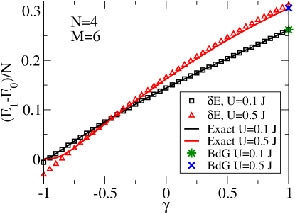
Figure 3: Solid lines represent the exact first excitation energy for $U=0.1J$ (black) and $U=0.5J$ (red). Squares and triangles, first excitation energy computed from Eqs. (23) and (25), replacing $q$ and $p$ by $0$ and $1$. Note also that for $-1<\gamma<1$ the ground and first excited states change symmetry, see Fig. 1. The cross and star symbols are the more accurate Bogoliubov-de Gennes predictions for $\gamma=1$. In all cases, $N=4$ and $M=6$.

We will now assume that to a good approximation, even when $U\neq 0$, the simplest excited states can be approximated as one atom being promoted from the coherent state $|\Psi_{q}^{(N)}\rangle$ made of all the atoms occupying the $\chi_{q}$ to an excited orbital $\chi_{p}$, both $p$ and $q$ orbitals being eigenstates of the non-interacting single particle Hamiltonian,

$$|\Psi_{q}^{(N-1)}\psi_{p}\rangle\equiv\frac{1}{\sqrt{(N-1)!}}(\hat{b}_{q}^{{\dagger}})^{N-1}\hat{b}_{p}^{{\dagger}}|\mbox{vac}\rangle\,.$$ (21)

The expectation value of the Hamiltonian (1) is the sum of the expectation value of the kinetic term and the interactions. The former element is:

$$\langle\Psi_{q}^{(N-1)}\psi_{p}|{\hat{\cal T}}|\Psi_{q}^{(N-1)}\psi_{p}\rangle=-J\,\left(\sum_{\lambda=1}^{M-1}\chi_{p}^{*}(\lambda+1)\chi_{p}(\lambda)+\gamma\chi_{p}^{*}(M)\chi_{p}(1)+{\rm c.c.}\right)$$

$$-J\,(N-1)\left(\sum_{\lambda=1}^{M-1}\chi_{q}^{*}(\lambda+1)\chi_{q}(\lambda)+\gamma\chi_{q}^{*}(M)\chi_{q}(1)+{\rm c.c.}\right)\,.$$ (22)

The kinetic energy cost of the promotion of one particle from the $q$ mode coherent ground state to the $p$ mode is:

$$\delta T \equiv \langle\Psi_{q}^{(N-1)}\psi_{p}|{\hat{\cal T}}|\Psi_{q}^{(N-1)}\psi_{p}\rangle-\langle\Psi_{q}^{(N)}|{\hat{\cal T}}|\Psi_{q}^{(N)}\rangle$$ (23)

$$= -J\bigg{[}\sum_{\lambda=1}^{M-1}\left(\chi_{p}^{*}(\lambda+1)\chi_{p}(\lambda)-\chi_{q}^{*}(\lambda+1)\chi_{q}(\lambda)\right)$$

$$+\gamma(\chi_{p}^{*}(M)\chi_{p}(1)-\chi_{q}^{*}(M)\chi_{q}(1))+{\rm c.c.}\bigg{]}\,.$$

A similar procedure can be followed to obtain the expectation value of $\hat{\cal U}$

$$\langle\Psi_{q}^{(N-1)}\psi_{p}|{\hat{\cal U}}|\Psi_{q}^{(N-1)}\psi_{p}\rangle = \frac{U}{2}\bigg{[}(N-1)(N-2)\sum_{\lambda=1}^{M}|\chi_{q}(\lambda)|^{4}$$ (24)

$$+ 4(N-1)\sum_{\lambda=1}^{M}|\chi_{q}(\lambda)|^{2}|\chi_{p}(\lambda)|^{2}\bigg{]}$$

together with the excitation energy cost due to interactions $\delta U\equiv\langle\Psi_{q}^{(N-1)}\psi_{p}|{\hat{\cal U}}|\Psi_{q}^{(N-1)}\psi_{p}\rangle-\langle\Psi_{q}^{(N)}|{\hat{\cal U}}|\Psi_{q}^{(N)}\rangle$, which yields to

$$\delta U\equiv U(N-1)\sum_{\lambda=1}^{M}\bigg{[}|\chi_{q}(\lambda)|^{2}(2|\chi_{p}(\lambda)|^{2}-|\chi_{q}(\lambda)|^{2})\bigg{]}\,.$$ (25)

Figure 3 shows the calculated lowest excitation energy, $\delta E=\delta T+\delta U$ for a range of values of $\gamma$ and two particular values of $U$. In addition, at $\gamma=1$ the energy gap predicted by the Bogoliubov-de Gennes approach computed as in Eqs. (20) and (21) of [27] has been added (cross for $U=0.5\ J$ and star for $U=0.1\ J$). The figure shows that for small values of $U$ and except in the vicinity of $\gamma=-1$ the present approximation can explain most of the effect of the interaction. The singular point $\gamma=-1$ will be discussed in the next Section.

5 Macroscopic superposition of superconducting flows when $\gamma=-1.$

5.1 Two-orbital approximation for the ground state manifold

As explained above, the non-interacting ground state for the $\gamma=-1$ configuration has a two-fold degeneracy between the two semifluxon states. In Ref. [32], it has been shown that for $M=3$ and small interactions, the low-energy states of the system can be described by a two-mode model involving only these two single-particle states. For a closed chain with $M$ sites, one can expect that the description of the system as a macroscopic superposition of two countercirculating semifluxons can be generalized. Moreover, the single-particle energy gap of Eq. (12) can be expected to protect the persistent currents created in the ground state manifold in ultracold atomic physics experiments. For $M\lesssim 8$ the gap is of the order of the tunnelling $J$. Thus, for few sites and small interactions ($NU\lesssim J$), the physics can be restricted to the degenerate ground state manifold.

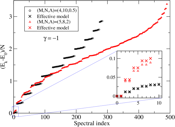
Figure 4: Exact many-body energy spectrum (with respect to the ground state energy) for $(M,N,\Lambda)=(4,10,0.5)$ (black circles) and $(5,8,2)$ (red triangles), in a closed BH chain with $\gamma=-1$. The inset compares the exact spectrum with the predicted values using the effective model in Eq. (27) (black and red crosses).

One can generalize the procedure followed in Ref. [32], by writing the creation and annihilation operators in the coherent flow basis, and truncating such decomposition to the semifluxon (sf) and the antisemifluxon (asf) states, i.e.,

$$\hat{a}^{{\dagger}}(\lambda)=\frac{1}{\sqrt{M}}\left(e^{i\lambda\pi/M}\,\hat{b}^{{\dagger}}_{\rm sf}+e^{-i\lambda\pi/M}\,\hat{b}^{{\dagger}}_{\rm asf}\right)$$ (26)

and the corresponding expression for $\hat{a}(\lambda)$. One can then rewrite the $\hat{\cal U}$ operator by taking into account that sums like $\sum_{\lambda=1}^{M}$ exp$(i2\lambda\pi/M)$ vanish, as

$$\hat{\cal U}={U\over 2M}\left[\hat{N}^{2}_{\rm sf}+\hat{N}^{2}_{\rm asf}+4\hat{N}_{\rm sf}\hat{N}_{\rm asf}-(\hat{N}_{\rm sf}+\hat{N}_{\rm asf})\right]\,,$$ (27)

where $\hat{N}_{x}=\hat{b}^{\dagger}_{x}\hat{b}_{x}$ with $x={\rm sf}$ or $x={\rm asf}$ are the number operators of semifluxon or antisemifluxon states. Since $N=N_{\rm sf}+N_{\rm asf}$ is constant, the last term in Eq. (27) corresponds to a global energy shift that can be neglected. The eigenstates of $\hat{\cal U}$ are the new “Fock” states

$$|N_{\rm sf},N_{\rm asf}\rangle=\frac{1}{\sqrt{N_{\rm sf}!N_{\rm asf}!}}(\hat{b}^{\dagger}_{\rm sf})^{N_{\rm sf}}(\hat{b}^{\dagger}_{\rm asf})^{N_{\rm asf}}|{\rm vac}\rangle\,.$$ (28)

In Fig. 4 we plot the energy spectrum obtained by exact diagonalization of the many-body Hamiltonian, Eq. (1). The band structure of the energy spectrum for small interactions, $\Lambda\lesssim 1$, can be understood by means of the number of atoms and the degeneracy of the flow basis elements (see A). In the figure we show two sets of parameters $(M,N,\Lambda)$ corresponding to $(4,10,0.5)$ and $(5,8,2)$. The spectrum of the first set shows traces of the degeneracy pattern present in the non-interacting case whereas for the second set the gaps close in the middle and slightly in the upper part of the spectrum. The inset in Fig. 4 shows the comparison between the low-lying exact many-body spectrum with the prediction of Eq. (27). This approximation turns out to be very accurate for small interactions $\Lambda<2$. For the two cases considered in the inset one can see that the model provides a good description for $\Lambda=0.5$, but it starts to deviate for larger values, such as $\Lambda=2$.

For small $\Lambda$, the eigenvectors belonging to the low energy manifold can be well approximated by

$$|\Psi_{k}^{\pm}\rangle={1\over\sqrt{2}}(|k,N-k\rangle\pm|N-k,k\rangle)\,,$$ (29)

using the Fock basis, $|N_{\rm sf},N_{\rm asf}\rangle$. The integer index $k$ runs from $0$ to $N$, and the $\pm$ sign labels the two states, which would be degenerate in energy if Eq. (27) was exact. In this approximation, $|\Psi_{0}^{\pm}\rangle$ corresponds to the two-fold degenerate ground state. A similar two-orbital approximation and macroscopic superposition of superfluid flow was considered in Ref. [33] for a three well system in a different gauge.

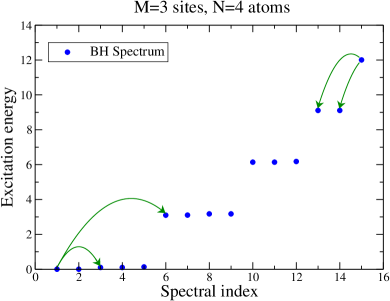
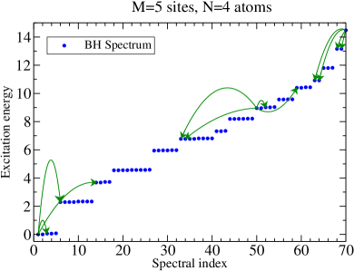
Figure 5: The blue dots indicate the exact many-body spectrum in a closed BH chain with $\gamma=-1$, for $(M,N,\Lambda)=(3,4,0.4)$ (left), and $(5,4,0.4)$ (right). The green arrows, which emerge from coherent mean-field states, account for the transitions predicted by the BdG excitations, Eq. (30).

5.2 Bogoliubov-de Gennes spectrum

The spectrum of elementary excitations in the weakly interacting regime can be studied within the Bogoliubov-de Gennes (BdG) framework. We follow the model presented in Ref. [27] for a circular array of Bose-Einstein condensates with the same tunnelling rate between the sites ($\gamma=1$). For the case of $\gamma=-1$, the equations are formally the same but with $\phi_{q}=\frac{2\pi}{M}(q+\frac{1}{2})$ instead of $\phi_{q}=\frac{2\pi}{M}q$ (see the discussion below Eq. (7)).

The Bogoliubov excitation spectrum is constructed over mean-field states defined as macroscopically occupied modes in the flow basis, Eq. (15), with $q=-1,0,1,\dots,M-2$ (or equivalently $q=0,1,\dots,M-1$). In the previous expression the corresponding coefficients of the creation operator $\hat{b}_{q}^{\dagger}$ are ${\tilde{\chi}}_{q}(\lambda;\gamma=-1)$ defined in Eq. (11). The periodicity of the system imposes that $q$ is a cyclic index, with period $M$: for example, $q=0\,(-1)$ and $M\,(M-1)$ are equivalent.

The excitation energies relative to a macroscopically occupied state can be obtained with the same procedure developed in Ref. [27]:

$$E_{k}^{(\pm)}=2J\sin\left(\frac{2\pi k}{M}\right)\sin(\phi_{q})\pm\sqrt{\varepsilon_{k}\left(\varepsilon_{k}+\frac{2(N-1)\,U}{M}\right)}\,,$$ (30)

with

$$\varepsilon_{k}=2J\cos(\phi_{q})\left[1-\cos\left(\frac{2\pi}{M}k\right)\right]\,.$$ (31)

The cyclic index $k$ runs from $0$ to $M-1$, and it is interesting to note that when $k=0\,(M)$, the Bogoliubov spectrum yields $E_{k=0}^{(\pm)}=0$, which corresponds to remain in the unperturbed mean-field state (without any excitation).

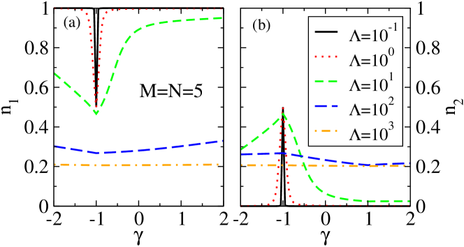
Figure 6: (a) Largest eigenvalue of the one-body density matrix, the condensed fraction $n_{1}$. (b) Second largest eigenvalue of the one-body density matrix $n_{2}$. The plots correspond to the case of $M=N=5$. The curves have been calculated for values of $\Lambda$ that range from $10^{-1}$ to $10^{3}$, and all of them are represented as a function of $\gamma$.

Figure 5 shows the exact many-body spectrum and the BdG excitations (indicated by arrows) relative to the mean-field like states of a system of $N=4$ atoms in $M$ sites. We have calculated the BdG spectrum in a chain with $M=3$ and $M=5$ sites with $\gamma=-1$ and for small interactions $U=0.1\,J$. The results are further discussed in B and collected in Tables 3 and 4. From the two possible excitations $E_{k}^{(\pm)}$ provided by the BdG calculation one has to discard the solution that does not fulfill the BdG normalization condition [27] (crossed as 3.55753 in Tables 3 and 4). Moreover, the solutions must fulfill that the excitations relative to the ground state are positive, whereas those relative to the highly excited macroscopically occupied state in the highest band must be negative.

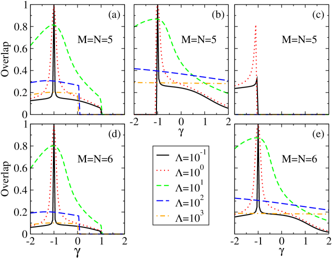
Figure 7: Absolute value of the overlap determinant, Eq. (32) for $M=N=5$ (a) and $M=N=6$ (d). (b) $|\langle\Psi_{\rm gs}^{(N)}|\Psi_{0}^{+}\rangle|$ for $M=N=5$. In the case $M=N=6$, $|\langle\Psi_{\rm gs}^{(N)}|\Psi_{0}^{+}\rangle|\lesssim 10^{-7}$ and is therefore not plotted. (c) and (e) depict $|\langle\Psi_{\rm gs}^{(N)}|\Psi_{0}^{-}\rangle|$ for $M=N=5$, and $M=N=6$, respectively. The curves have been calculated for values of $\Lambda$ that range from $10^{-1}$ to $10^{3}$, and all of them are represented as a function of $\gamma$.

6 Robustness of superconducting flows when $\gamma\neq-1$

The macroscopic superpositions of semifluxon states are predicted to appear for low interactions in the special $\gamma=-1$ case. Our focus here will be on studying the presence of such macroscopic superpositions of superfluid flows when $\gamma\neq-1$. Two indicators will be used to signal the presence of macroscopic cat-like states as the ones written in Eq. (29) with $k=0$. The first one is the overlap between the cat states and the exact solutions resulting from the numerical diagonalization. As discussed earlier, for $\Lambda\lesssim 1$ the ground state is almost doubly degenerate, then, $\{|\Psi_{0}^{+}\rangle,|\Psi_{0}^{-}\rangle\}$ is a suitable basis for the lower manifold, as predicted by the two-orbital model. We therefore define the overlap determinant as,

$${\cal O}=\left|\left(\matrix{\langle\Psi_{\rm gs}^{(N)}|\Psi_{0}^{+}\rangle&\langle\Psi_{\rm gs}^{(N)}|\Psi_{0}^{-}\rangle\cr\langle\Psi_{\rm 1st}^{(N)}|\Psi_{0}^{+}\rangle&\langle\Psi_{\rm 1st}^{(N)}|\Psi_{0}^{-}\rangle\cr}\right)\right|\,,$$ (32)

with $|\Psi_{\rm gs}^{(N)}\rangle$ and $|\Psi_{\rm 1st}^{(N)}\rangle$ the ground and first excited states obtained by direct diagonalization, respectively. The overlap ${\cal O}$ is $1$ when the two manifolds are the same.

The second indicator is the fragmentation of the ground state of the system, given by the eigenvalues $n_{i}$ of the single-particle density matrix, $\hat{\rho}^{(1)}_{ij}=\langle\Psi|\hat{a}_{i}^{\dagger}\hat{a}_{j}|\Psi\rangle/N$, with $i,j=1,\dots,M$. The eigenvalues fulfill $\sum_{i}n_{i}=1$, and the largest one is called the condensed fraction of the system. A fully condensed many-body state has $n_{1}=1$. Instead, the two macroscopic superpositions in Eq. (29) are bifragmented and produce $n_{1}=n_{2}=1/2$. A Mott-insulating phase with integer filling has $n_{i}=1/M$, for $i=1,\dots,M$.

As expected, the values of the overlap determinant are clearly correlated with those of the condensed fraction, see Figs. 6, 7 and 8. The system is found to be approximately bifragmented when there is a noteworthy overlap determinant. For small $\Lambda$ and $\gamma=-1$ we find both condensed fractions $n_{1}\simeq n_{2}\simeq 1/2$ and an overlap determinant very close to $1$, regardless of the number of particles and filling factor, $N/M$. What is somewhat unexpected is that finite values of $\Lambda$ enhance the probability of finding these macroscopic superposition states when $\gamma\neq-1$. For fixed $M$ and filling factors below $1$, the area covered by the significantly fragmented configurations broadens for increasing filling, as seen comparing the $(M,N)=(10,3)$, $(10,4)$, and $(10,5)$ panels in Fig. 8. For filling factors larger than one, the fragmented region gets reduced, see panels $(M,N=M)$ and $(M,N=2M)$ in Fig. 8.

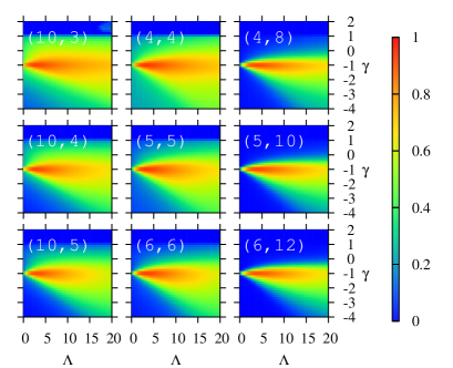
Figure 8: The condensed fraction $n_{1}$ (left panels) and the overlap determinant $\mathcal{O}$ (right panels) are represented in a color map as a function of $\gamma$ and $\Lambda$, for different values of the pair $(M,N)$, which appears as a label in each plot. From top to bottom, the left column has increasing filling factor from $3/10$ to $1/2$, and the middle and right columns have increasing number of sites $M$ for filling factor $1$ and $2$, respectively.

Note that the overlap determinant would be strictly zero if the quasi degeneracy is absent. In this case, even though the ground state may still be well described by $|\Psi_{0}^{+}\rangle$, we would get a zero overlap between the two manifolds. This is the reason why the overlap becomes abruptly zero in the vicinity of $\gamma=1$ signalling a level crossing in the many-body spectrum between the first and second excited states, see Figs. 7 and 8. This level crossing is directly related to the crossing found at $\gamma=1$ in the single-particle spectrum, see Fig. 2. Even though the two-fold degeneracy is broken, we find that the actual ground state of the system has a sizeable overlap with the $|\Psi_{0}^{+}\rangle$ state in a broader region of parameters, as seen in Fig. 7(b). There, for $N=M=5$ we find that $\Lambda\simeq 1$ is a good candidate to find counterflow cat states for a broad range of $\gamma$. The overlaps between the ground state and the two quasi-degenerate cat states in the vicinity of $\gamma=-1$ depend critically on the number of particles. In the case $N=M=5$ for $\gamma\simeq-1$ we find that the overlap between the ground state and $|\Psi_{0}^{+}\rangle$ goes from almost one for $\gamma\gtrsim-1$ to close to zero for $\gamma\lesssim-1$ for $\Lambda\lesssim 1$. While the situation is the opposite for the overlap with $|\Psi_{0}^{-}\rangle$. A much more symmetric situation is found for even number of particles, which does not show this change, as seen in Fig. 7(d,e). This behaviour can be understood from the two-orbital description of Sect. 5.1, details are beyond the scope of the present manuscript.

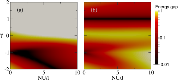
Figure 9: (a) Energy gap between the many-body ground state and the first excited state, and (b) energy difference between the first and second excited states. Both are computed as a function of $\Lambda$ and $\gamma$ for $N=M=5$.

Further increasing the interactions, $\Lambda>100$, the condensed fraction decreases quickly to the expected value $1/M$ for the Mott insulating regime, Fig. 6. For integer filling, in the $\Lambda\to\infty$ limit the ground state is non-degenerate and gapped (Mott insulator of the corresponding filling). Thus, it is expected that already for any finite value of $\Lambda$ the two-fold degeneracy predicted by the two orbital model would be only approximate. For fractional fillings, in contrast, in the large interaction limit the ground state will be degenerate, with the surplus particles delocalized in the chain. In this case the numerics shows that the two-fold degeneracy predicted by our model is present for all values of $\Lambda$.

Besides the condensed fraction and the overlap, a crucial feature of a macroscopic superposition is its robustness, characterized by the presence of an energy gap that protects the superposition to be affected by excitations that could involve larger-energy excited states. In Fig. 9 we present the energy difference between the ground state and the first excited state, panel (a), and the energy difference between the latter and the second excited one, panel (b). There are two important properties exhibited by the peculiar case of $\gamma=-1$. First, for zero interactions, the ground state has a very large degeneracy, $N+1$, stemming from the combinatorial factor, i.e. $N$ particles populating two single-particle states in $N+1$ ways, see A. For very small interactions, $\Lambda\lesssim 0.5$, this is reflected in the very small gap $\lesssim 0.01\,J$ both between the ground and first, see Fig. 9(a), and between the first and second excited many-body eigenstates, see Fig. 9(b). Secondly, for $\gamma=-1$ and $\Lambda\gtrsim 5$, a gap starts to open above the ground state. This gap opening increases the robustness of the macroscopic superposition, which indicates that experimental observation of these states should be feasible.

When $U=0$ the densities can be easily constructed using the wavefunctions given by Eq. (4). When $\gamma>-1$, the ground state is symmetric, see Fig. 1, and the density is given by,

$$\rho^{\gamma}(\lambda)=\frac{N}{\cal{N}_{+}}\ \cos^{2}\left[\left(\frac{M+1}{2}-\lambda\right)\phi\right]\,,$$ (33)

with $\phi$ determined from Eq. (5). These densities are linear in $N$, have a maximum at $\lambda_{m}=(M+1)/2$ and are site symmetric with respect to $\lambda_{m}$. The simplest example is the case $\gamma=0$: then the solution of Eq. (5) is $\phi=\pi/(M+1)$ and

$$\rho^{\gamma=0}(\lambda)=\frac{2N}{M+1}\ \sin^{2}\left(\frac{\pi}{M+1}\lambda\right)\,,$$ (34)

which shows that at the maximum $\rho_{M}=2N/(M+1)$ and at sites $1$ and $M$, $\rho=2N/(M+1)\sin^{2}(\pi/(M+1))$. Analogous expressions, involving hyperbolic functions, can be easily derived for the surface states.

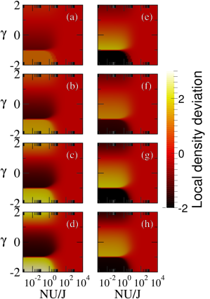
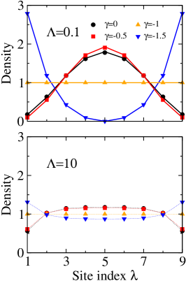
Figure 10: (left panels) Deviation of the local density of the ground state from its global average at the tunable link (a-d), and in the center of the chain, furthest from the tunable link (e-h) as a function of $\Lambda\equiv NU/J$ and $\gamma$. The filling factor is the same for all panels, $N/M=2$. $M=3$, 4, 5 and 6, are depicted in panels (a,e), (b,f), (c,g) and (d,h), respectively. (right panels) Local average density of the ground state, $\langle\hat{a}^{\dagger}(\lambda)\hat{a}(\lambda)\rangle$, as a function of the site index $\lambda$ for $N=M=9$. Symbols depict the exact results for the values of $\gamma=-1.5$ (down-triangles), $-1$ (up-triangles), $-0.5$ (squares) and $0$ (circles). For the small interaction case, $\Lambda=0.1$, we add the non-interacting result, given explicitly in Eq. (33) for bulk states, as solid lines. The dotted lines for $\Lambda=10$ are just linear interpolations of the exact results.

Similar expressions can be written when $\gamma<-1$, now using the odd single-particle solutions. The exact results shown in Fig. 10 for $\Lambda=0.1$ are almost identical to these simple predictions, except when $\gamma$ is very close to $-1$ where the breaking of the degeneracy of the odd and even solutions when $U\neq 0$ has to be taken into account.

The effect of varying $\gamma$ and $\Lambda$ on the density of the cloud is also particularly pronounced. For $\gamma=1$, the population is equal within all the sites, as the system is rotationally symmetric. For $\gamma=-1$ the situation is different due to the quasidegeneracy at the ground state level. For small values of the interaction, the ground state is well represented by the cat states (29), which have an equal amount of fluxon and antifluxon components resulting also in a constant density along the chain, see Fig. 10. In the Mott regime, the system is equipopulated again, regardless of the value of $\gamma$, see the $\Lambda\gtrsim 10$ results in Fig. 10. Already for $|\gamma|\gtrsim 1.5$, the density approaches the one built from the surface modes described in the first section, with population peaked on the sites around the tunable link. In Fig. 10 we provide a broader picture for filling factor $2$. Again for large interactions, both the central density and the density at the extremes approach the $N/M=2$ limit. Interestingly, the region of macroscopic superposition of fluxon-antifluxon states reflects in an almost equipopulation of all sites for all values of $\Lambda$. As discussed above, away from $\gamma=-1$ and for lower interactions, the cat-like state is less robust, resulting in a higher density in the center (extremes) as $\gamma$ increases (decreases). Monitoring the density of the chain can therefore be a good indicator of the macroscopic superposition states expected. For instance, the chain could be initially prepared at small but nonzero interactions and $\gamma=1$. Turning the tunable link from $\gamma=1$ to $\gamma=-1$, the density in the center will grow, reaching very large values for $\gamma\simeq-1$. At $\gamma=-1$ the chain should again be equipopulated. This transition from having almost zero population in the extremes to equipopulation would signal the regime of macroscopic superposition of fluxon-antifluxon states.

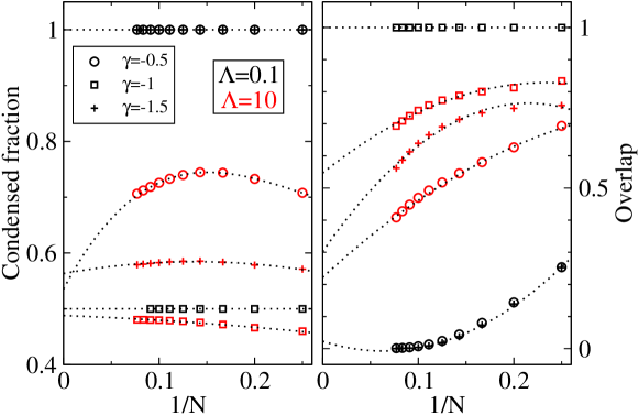
Figure 11: Condensed fraction (left panel) and overlap determinant (right panel), for $\gamma=-0.5$ (circles), $-1$ (squares) and $-1.5$ (crosses), with $\Lambda=0.1$ (black) and $\Lambda=10$ (red), as a function of $1/N$. The filling factor is one in all cases, and the maximum number of particles reached is $N=M=13$. The dotted lines depict a quadratic extrapolation of the calculated points to the thermodynamic limit ($N\to\infty$).

The transition from a condensed to a fragmented state consisting in a macroscopic superposition of counterpropagating flows has been described for finite number of particles and sites using exact diagonalization techniques. It has been shown to take place at small but nonzero interactions, which actually helps to stabilize the superposition. Now we will stretch our numerical diagonalization techniques to explore the thermodynamic limit at small $\Lambda$. We have used the ARPACK package to go up to Hilbert spaces of dimension $\simeq 10^{6}$. This allows us to explore the behaviour of the macroscopic superpositions of semifluxon states with up to $N=M=13$, as shown in Fig. 11. To roughly explore the thermodynamic limit we have performed extrapolations using up to quadratic terms in $1/N$, shown in the figure with dotted lines. The transition to the macroscopic superposition phase is clearly seen to be much more robust at $\Lambda=10$ than $\Lambda=0.1$. In the former, for instance we find values of the overlap determinant of about $0.25$ for $\gamma=-0.5$, $-1$ and $-1.5$ in the extrapolation to the thermodynamic limit. The corresponding ground state fragmentation is close to $0.5$ in agreement with the predicted bifragmented nature of the superposition state. For smaller $\Lambda$ the superposition is only found at values $\gamma\simeq-1$: departures from it lead to a quick loss of the bifragmentation and to small values of the overlap determinant.

7 Summary and conclusions

In this paper we have studied the role of a tunable link in a Bose-Hubbard chain of arbitrary size. In the case of non-interacting closed systems, we find counterpropagating persistent current states in the upper part of the spectrum with $\gamma=1$ [34], and in the ground state for the case of $\gamma=-1$, constituting a cat state of macroscopic flows. In this latter case, we have also analyzed the Bogoliubov excitations over mean-field states when interaction is present, by following a procedure similar to the one presented in Ref. [27].

We have analyzed the robustness of these counterflow cat states by studying the energy spectrum, the density profile, the condensed fraction and the overlap of the non-interacting ground state manifold with the ground state computed by exact diagonalization, as a function of the interaction and $\gamma$. We have found that macroscopic superpositions of counterflow in weakly interacting Bose gases in a closed Bose-Hubbard chain with $\gamma=-1$ is more robust against fluctuation of the parameters, and is protected by a larger energy gap from excited states. Quadratic extrapolation to the large $N$ limit in the filling factor $N/M=1$ regime predicts the existence of such superpositions in the thermodynamic limit for small but non-zero interactions, $\Lambda\lesssim 5$.

The production of macroscopic superpositions of semifluxon states in interacting many-body systems opens a new possibility to obtain persistent currents which may be useful in quantum computation and quantum simulation. An important feature of the results described in this article is that they are applicable to rings of any number of sites and thus can be engineered in a large variety of experimental setups. Thus, closed Bose-Hubbard chains with a single tunable link provide a versatile system in which macroscopic superpositions of flow states can be produced with a tunable twisted link, in which the tunnelling can be varied both in strength and phase. Among the possibilities that exist nowadays, cold atoms [35] and coupled non-linear optical resonators [36] are promising quantum devices to produce countersuperflow states.

8 Acknowledgments

We acknowledge financial support from the Spanish MINECO (FIS2014-52285-C2-1-P and FIS2014-54672-P) and from Generalitat de Catalunya Grant No. 2014SGR401. A. G. is supported by Spanish MECD fellowship FPU13/02106. B. J-D. is supported by the Ramón y Cajal MINECO program.

Appendix A Many-body spectrum for weakly interacting systems: band structure when $\gamma=\pm 1$

In addition to the usual site basis for single bosons, it is convenient to consider also the flow basis that incorporates the matching condition, see Eq. (16):

$$|{\tilde{\psi}}_{q}\rangle = {\tilde{b}}^{{\dagger}}_{q}\,|{\rm vac}\rangle$$ (35)

$$= \frac{1}{\sqrt{M}}\sum_{l=0}^{M-1}e^{i\,l\phi_{q}}\,\hat{a}_{l}^{\dagger}\,|{\rm vac}\rangle\,,$$

where $\phi_{q}=\frac{2\pi}{M}q$ for $\gamma=1$, and $\phi_{q}=\frac{2\pi}{M}(q+\frac{1}{2})$ for $\gamma=-1$,with $q=0,1,...,M-1$. Since $e^{i\,l\phi_{q}}$ is a periodic function, $q$ is a cyclic index with period $M$.

For example, for a trimer $M=3$ with $\gamma=1$, the flow basis, see Eq. (11), expressed in the Fock states (number of particles per each site), is:

$$|0\rangle = {1\over\sqrt{3}}\left(|1,0,0\rangle+|0,1,0\rangle+|0,0,1\rangle\right)$$ (36)

$$|{\rm fl}\rangle = {1\over\sqrt{3}}\left(|1,0,0\rangle+e^{i{2\pi\over 3}}|0,1,0\rangle+e^{i{4\pi\over 3}}|0,0,1\rangle\right)$$

$$|{\rm afl}\rangle = {1\over\sqrt{3}}\left(|1,0,0\rangle+e^{-i{2\pi\over 3}}|0,1,0\rangle+e^{-i{4\pi\over 3}}|0,0,1\rangle\right)\,.$$

The basis elements correspond to equipartition of an atom in the three sites with zero flow, $|0\rangle$, a vortex state with clockwise flow $2\pi$ (fluxon), $|{\rm fl}\rangle$, and an anti-vortex (antifluxon) state, $|{\rm afl}\rangle$, with counterclockwise flow $-2\pi$. Conversely, the $N$ boson Fock states in this basis are $|N_{0},N_{\rm fl},N_{\rm afl}\rangle$, where $N_{0},N_{{\rm fl}}$ and $N_{{\rm afl}}$ are the number of atoms in the $|0\rangle,|{\rm fl}\rangle$ and $|{\rm afl}\rangle$ flow states, respectively. It is important to stress that clockwise and counterclockwise states, $|{\rm fl}\rangle$ and $|{\rm afl}\rangle$ are degenerate since there is not a fixed rotation direction in the hamiltonian.

In the case of a trimer with $\gamma=-1$, the flow basis, Eq. (11), is:

$$|{\rm sf}\rangle = {1\over\sqrt{3}}\left(|1,0,0\rangle+e^{i{\pi\over 3}}|0,1,0\rangle+e^{i{2\pi\over 3}}|0,0,1\rangle\right)$$

$$|{\rm asf}\rangle = {1\over\sqrt{3}}\left(|1,0,0\rangle+e^{-i{\pi\over 3}}|0,1,0\rangle+e^{-i{2\pi\over 3}}|0,0,1\rangle\right)$$

$$|{\rm sfl+fl}\rangle = {1\over\sqrt{3}}\left(|1,0,0\rangle+e^{i\pi}|0,1,0\rangle+e^{i2\pi}|0,0,1\rangle\right)$$ (37)

$$= {1\over\sqrt{3}}\left(|1,0,0\rangle-|0,1,0\rangle+|0,0,1\rangle\right)\,.$$

Here, the states $|\rm sf\rangle$ and $|{\rm asf}\rangle$ are degenerate and correspond to a half-vortex (or semifluxon) and an anti-half-vortex (antisemifluxon) state with clockwise and counterclockwise flow $\pm\pi$, respectively. The third basis element $|{\rm sf+fl}\rangle$ is an excited state with clockwise flow which carries one and a half quantum flux of a vortex state: $3\pi$.

In this flow basis a general Fock state is given by $|N_{\rm sf},N_{\rm asf},N_{\rm sf+fl}\rangle$, where $N_{\rm sf},N_{\rm asf}$ and $N_{\rm sf+fl}$ are the number of atoms in the $|{\rm sf}\rangle,|{\rm asf}\rangle$ and $|{\rm sf+fl}\rangle$ flow states, respectively.

In a Bose-Hubbard chain with $M=5$ sites and $\gamma=-1$, there are 5 elements in the flow basis: $|{\rm sf}\rangle\equiv|{\tilde{\psi}}_{0}\rangle$ and $|{\rm asf}\rangle\equiv|{\tilde{\psi}}_{-1}\rangle$ are degenerate and correspond to semifluxon and antisemifluxon states, respectively; $|{\rm sf+fl}\rangle\equiv|{\tilde{\psi}}_{1}\rangle$ and $|{\rm asf+afl}\rangle\equiv|{\tilde{\psi}}_{3}\rangle$ that are degenerate and carry $\pm 3\pi$ flux; and $|{\rm sf+2fl}\rangle\equiv|{\tilde{\psi}}_{2}\rangle$ which is a non-degenerate state that carries $5\pi$ clockwise flow.

The band structure of the non-interacting spectrum and also for small interactions $\Lambda<1$, see Figs. 4 and  5, can be understood by means of the number of sites, the number of atoms, and the degeneracy of the flow basis elements.

For example for $M=3$ sites and $\gamma=-1$ the single-particle spectrum has a ground state with two degenerate eigenvectors, $|{\rm fl}\rangle$ and $|{\rm afl}\rangle$, and an excited state $|{\rm sf+fl}\rangle$. For a system with $N$ atoms, the total number of bands is $N+1$ that corresponds to the different possibilities of distributing $N$ atoms in a two level system with occupancies $N_{1/2}\equiv N_{\rm sf}+N_{\rm asf}$ and $N_{3/2}\equiv N_{\rm sf+fl}$, with the restriction $N=N_{1/2}+N_{3/2}$. Inside each band, the number of quasi-degenerate levels can be calculated by counting the number of different possibilities $(N_{\rm sf},N_{\rm asf})$ to set $N_{1/2}$ atoms between two degenerate levels $|{\rm sf}\rangle$ and $|{\rm asf}\rangle$, where $N_{1/2}\equiv N_{\rm sf}+N_{\rm asf}$. The quasi-degeneration is $deg_{1/2}=N_{1/2}+1$.

In tables 1 and 2 we present the distribution in bands and the quasi-degeneracy inside each band, for the many-body spectrum of $N$ weakly-interacting atoms in $M$ sites.

Figure 5 shows the band structure of the exact many-body spectrum for $N=4$ atoms in $M=3$ and $M=5$ sites, for small interactions. The band degeneracy predicted in Table 1 and 2 is in agreement with the quasi-degeneracy inside each band obtained numerically (see Fig. 5).

$M=3,N=4$	band 1	band 2	band 3	band 4	band 5
$N_{1/2}=N_{\rm sf}+N_{\rm asf}$	4	3	2	1	0
$(N_{\rm sf},N_{\rm asf})$	(4,0)	(3,0)	(2,0)	(1,0)	(0,0)
	(0,4)	(0,3)	(0,2)	(0,1)	(0,0)
	(3,1)	(2,1)	(1,1)
	(1,3)	(1,2)	(1,1)
	(2,2)
$deg_{1/2}=N_{1/2}+1$	5	4	3	2	1
$N_{3/2}=N_{\rm sf+fl}$	0	1	2	3	4
$deg_{3/2}$	1	1	1	1	1
band degeneracy	5	4	3	2	1
$deg=deg_{1/2}\times deg_{3/2}$

Table 1: Distribution of $N=4$ atoms in the single-particle flow states of $M=3$ sites with $\gamma=-1$: $|{\rm sf}\rangle$, $|{\rm asf}\rangle$ and $|{\rm sf+fl}\rangle$. The many-body states in the flow basis are $|N_{\rm sf},N_{\rm asf},N_{\rm sf+fl}\rangle$. The mean-field like states are marked in boldface and correspond to: $|4,0,0\rangle,|0,4,0\rangle,|0,0,4\rangle$.

$M=5,N=4$	b1	b2	b3	b4	b5	b6	b7	b8	b9	b10	b11	b12	b13	b14	b15
$N_{1/2}=N_{\rm sf}+N_{\rm asf}$	4	3	3	2	2	1	2	1	0	1	0	1	0	0	0
$(N_{\rm sf},N_{\rm asf})$	(4,0)	(3,0)	(3,0)	(2,0)	(2,0)	(1,0)	(2,0)	(1,0)	(0,0)	(1,0)	(0,0)	(1,0)	(0,0)	(0,0)	(0,0)
	(0,4)	(0,3)	(0,3)	(0,2)	(0,2)	(0,1)	(0,2)	(0,1)		(0,1)		(0,1)
	(3,1)	(2,1)	(2,1)	(1,1)	(1,1)		(1,1)
	(1,3)	(1,2)	(1,2)
	(2,2)
$deg_{1/2}=N_{1/2}+1$	5	4	4	3	3	2	3	2	1	2	1	2	1	1	1
$N_{3/2}=N_{\rm sf+fl}+N_{\rm asf+afl}$	0	1	0	2	1	3	0	2	4	1	3	0	2	1	0
$(N_{\rm sf+fl},N_{\rm asf+afl})$	(0,0)	(1,0)	(0,0)	(2,0)	(1,0)	(3,0)	(0,0)	(2,0)	(4,0)	(1,0)	(3,0)	(0,0)	(2,0)	(1,0)	(0,0)
		(0,1)		(0,2)	(0,1)	(0,3)		(0,2)	(0,4)	(0,1)	(0,3)		(0,2)	(0,1)
				(1,1)		(2,1)		(1,1)	(3,1)		(2,1)		(1,1)
						(1,2)			(1,3)		(1,2)
									(2,2)
$deg_{3/2}=N_{3/2}+1$	1	2	1	3	2	4	1	3	5	2	4	1	3	2	1
$N_{5/2}=N_{\rm sf+2fl}$	0	0	1	0	1	0	2	1	0	2	1	3	2	3	4
band degeneracy	5	8	4	9	6	8	3	6	5	4	4	2	3	2	1
$deg=deg_{1/2}\times deg_{3/2}$

Table 2: Distribution of $N=4$ atoms in the single-particle flow states of $M=5$ sites with $\gamma=-1$: $|\rm sf\rangle$, $|\rm asf\rangle$, $|\rm sf+fl\rangle$, $|\rm asf+afl\rangle$, $|\rm sf+2fl\rangle$. The many-body states in the flow basis are $|N_{\rm sf},N_{\rm asf},N_{\rm sf+fl},N_{\rm asf+afl},N_{\rm sf+2fl}\rangle$. The corresponding mean-field like states are marked in boldface and correspond to: $|4,0,0,0,0\rangle,|0,4,0,0,0\rangle,|0,0,4,0,0\rangle,|0,0,0,4,0\rangle$, and $|0,0,0,0,4\rangle$. This case corresponds to a three level system with occupancies $N_{1/2}$, $N_{3/2}$ and $N_{5/2}$ with $N=N_{1/2}+N_{3/2}+N_{5/2}$ and 15 bands.

Appendix B Detailed Bogoliubov analysis of $M=3$ and $M=5$ sites

In this appendix we provide a detailed analysis of the BdG spectrum for $M=3$ and $M=5$ sites at low interactions.

B.1 Case 1: M=3 sites

For $N$ atoms and $M=3$ sites, there are 3 macroscopically occupied states expressed in the Fock basis $|N_{\rm sf},N_{\rm asf},N_{\rm sf+fl}\rangle$ (see A), namely: $|{\tilde{\Psi}}_{q=0}^{(N)}\rangle=|N,0,0\rangle,\,$ $|{\tilde{\Psi}}_{q=-1}^{(N)}\rangle=|0,N,0\rangle$ and $|{\tilde{\Psi}}_{q=1}^{(N)}\rangle=|0,0,N\rangle$. The two first ones are degenerate and belong to the lowest band, and the latter is the unique state in the highest band. One can consider a small rotational bias to break the degeneracy, such as the many-body ground state of the system is either the macroscopically occupied semifluxon mode $|{\tilde{\Psi}}_{q=0}^{(N)}\rangle=|N,0,0\rangle$, or the anti-semifluxon mode $|{\tilde{\Psi}}_{q=-1}^{(N)}\rangle=|0,N,0\rangle$. When $M=3$, for a fixed mean-field state $|{\tilde{\Psi}}_{q}^{(N)}\rangle$, there are three possible values of the index $k=-1,0,1$, and therefore two elementary excitations $k=\pm 1$. In the BdG framework [27], they can be understood as the building up of a fluxon (vortex-like excitation) when $k=1$ or an antifluxon (antivortex-like excitation) when $k=-1$.

Let us consider the macroscopically occupied semifluxon mode $|{\tilde{\Psi}}_{q=0}^{(N)}\rangle=|N,0,0\rangle$, an excitation with $k=-1$ will lead the system to the excited state $|N-1,1,0\rangle$ which corresponds to the promotion of one particle from $|{\rm sf}\rangle$ to $|{\rm sf+fl}\rangle$, whereas a $k=1$ excitation will lead to the final state $|N-1,0,1\rangle$.

In Fig. 5 the BdG excitations are shown for a system with $M=3$, $N=4$ and $U/J=0.1$. When the macroscopically occupied mode is the semifluxon mode $|{\tilde{\Psi}}_{q=0}^{(N)}\rangle=|4,0,0\rangle$, a $k=-1$ excitation leads the system to the excited state $|3,1,0\rangle$ which is the third one in the lowest band, see Table 1 in A. The BdG excitation energy is $E_{k=-1}^{q=0}/J=0.0969$ which is in good agreement with the excitation energy calculated by exact diagonalization $\Delta E^{q=0}_{k=-1}/J=0.0992$ (see Table 3).

A $k=1$ excitation relative to $|{\tilde{\Psi}}_{q=0}^{(N)}\rangle=|4,0,0\rangle$, leads to the many-body state $|3,0,1\rangle$, whereas a $k=-1$ excitation leads to $|3,1,0\rangle$. Both final states are degenerate in the fourth band (see Fig. 5), and therefore the BdG prediction gives the same excitation energies $E_{k=1}^{q=0}/J=E_{k=-1}^{q=0}/J=3.0969$ in quantitative agreement with the exact excitation energy $\Delta E^{q=0}_{k=1}/J=3.0998$ (see Table 3).

$q$	$|{\tilde{\Psi}}_{q}^{N)}\rangle$	$k$	$E_{k}^{+}/J$	$E_{k}^{-}/J$	$\Delta E^{q}_{k}/J$	$|\Psi_{q,k}^{\prime}\rangle$
0	$|4,0,0\rangle$	-1	0.0969	-3.0969	0.0992	$|3,1,0\rangle$
		1	3.0969	-0.0969	3.0998	$|3,0,1\rangle$
-1	$|0,4,0\rangle$	-1	-3.0969	0.0969	0.0992	$|1,3,0\rangle$
		1	-0.0969	3.0969	3.0998	$|0,3,1\rangle$
1	$|0,0,4\rangle$	-1	2.8983	-2.8983	-2.8977	$|1,0,3\rangle$
		1	2.8983	-2.8983	-2.8977	$|0,1,3\rangle$

Table 3: Excitation energies of a macroscopically occupied mode $|{\tilde{\Psi}}_{q}^{(N)}\rangle$: $E_{k}^{(\pm)}$ obtained from the Bogoliubov framework at a given $q$, and $\Delta E^{q}_{k}$ obtained by exact diagonalization. The excitation energies from the ground state $(q=0$ and $q=1)$ must be positive, whereas from the highest excited mode $(q=1)$ they must be negative. $|{\tilde{\Psi}}_{q,k}^{\prime}\rangle$ is the resulting excited many-body state expressed in the Fock basis $|N_{sf},N_{\rm asf},N_{\rm sf+fl}\rangle$. $M=3,N=4,U/J=0.1$

In Table 3 we compare the excitation energies calculated within the BdG formalism and the ones obtained by exact diagonalization of the BH hamiltonian for $M=3$ and $N=4$ and $U/J=0.1$. As can be seen in the table, the agreement for weakly interacting systems is very good.

B.2 Case 2: $M=5$ sites

For $N$ atoms in a BH chain with $M=5$ sites the flow basis is $|N_{\rm sf},N_{\rm asf},N_{\rm sf+fl},N_{\rm asf+afl},N_{\rm sf+2fl}\rangle$. There are 5 macroscopically occupied states ($q=-1,0,1,2,3$), see Table 2 for $N=4$ atoms. Two of them are degenerate in the lowest band (b1): $|\Psi_{q=0}^{0}\rangle=|N,0,0,0,0\rangle$, and $|{\tilde{\Psi}}_{q=-1}^{(N)}\rangle=|0,N,0,0,0\rangle\,$; two are degenerate in a middle band (b9) $|{\tilde{\Psi}}_{q=1}^{(N)}\rangle=|0,0,N,0,0\rangle$, and $|{\tilde{\Psi}}_{q=3}^{(N)}\rangle=|0,0,0,N,0\rangle\,$; and the last one is the highest excited state in the last band (b15) $|{\tilde{\Psi}}_{q=2}^{(N)}\rangle=|0,0,0,0,N\rangle\,$. For a mean-field state, i.e. for a fixed $q$, the BdG framework will provides 5 possible excitation energies labeled by $k=-1,0,1,2,3$ (or an equivalent set of values due to the periodicity).

They can be understood as the building up of: a vortex-like excitation (fluxon) with $k=1$, an antivortex-like excitation (antifluxon) with $k=-1$, a doubly quantized vortex-like excitation (two fluxons) or equivalently three antifluxons with $k=2\,(-3)$, and three fluxons or equivalently two antifluxons with $k=3\,(-2)$.

Again, one can consider a small rotational bias such as the many-body ground state of the system is the macroscopically occupied semifluxon state $|{\tilde{\Psi}}_{q=0}^{(N)}\rangle=|N,0,0,0,0\rangle$. With another bias the ground state of the system can be $|{\tilde{\Psi}}_{q=-1}^{(N)}\rangle=|0,N,0,0,0\rangle$, that corresponds to the macroscopically occupied antisemifluxon state.

We have calculated the BdG excitations related to the macroscopically occupied states for $N=4$ atoms and $U/J=0.1$. In Table 4 we compare the BdG spectrum with the excitation energies obtained from the BH Hamiltonian. We have discarded all solutions which do not fulfill the BdG normalization [27]. From this comparison, it follows that the BdG framework provides a good description for low-lying excitation energies when the interactions are small.

$q$	$|{\tilde{\Psi}}_{q}^{(N)}\rangle$	$k$	$E_{k}^{+}/J$	$E_{k}^{-}/J$	$\Delta E^{q}_{k}/J$	$|{\tilde{\Psi}}_{q,k}^{\prime}\rangle$
0	$|4,0,0,0,0\rangle$	-1	0.0584	-2.2945	0.0590	$|3,1,0,0,0\rangle$
		1	2.2945	-0.0585	2.2913	$|3,0,1,0,0\rangle$
		2	3.6774	-2.2954	3.6797	$|3,0,0,0,1\rangle$
		-2 (3)	2.2954	-3.6774	2.2968	$|3,0,0,1,0\rangle$
1	$|0,0,4,0,0\rangle$	-1	-1.4469	-2.1711	-2.1828	$|1,0,3,0,0\rangle$
		1	2.1711	1.4469	1.4424	$|0,0,3,0,1\rangle$
		-3 (2)	2.1745	0.0617	0.0569	$|0,0,3,1,0\rangle$
		-2 (3)	-0.0617	-2.1744	-2.1822	$|0,1,3,0,0\rangle$
2	$|0,0,0,0,4\rangle$	-1	1.3206	-1.3206	-1.3205	$|0,0,1,0,3\rangle$
		-4 (1)	1.3206	-1.3206	-1.3205	$|0,0,0,1,3\rangle$
		-3 (2)	3.5575	-3.5575	-3.5583	$|0,1,0,0,3\rangle$
		-2 (3)	3.5575	-3.5575	-3.5583	$|1,0,0,0,3\rangle$

Table 4: Same as Table 3 for $M=5,N=4$ and $U/J=0.1$. In this case the many-body states $|{\tilde{\Psi}}_{q}^{(N)}\rangle$ and $|{\tilde{\Psi}}_{q,k}^{\prime}\rangle$ are expressed in the Fock basis $|N_{\rm sf},N_{\rm asf},N_{\rm sf+fl},N_{\rm asf+afl},N_{\rm sf+2fl}\rangle$.

References

- [1] Cazalilla M A, Citro R, Giamarchi T, Orignac E and Rigol M 2011 Rev. Mod. Phys. 83(4) 1405–1466 URL http://link.aps.org/doi/10.1103/RevModPhys.83.1405
- [2] Giamarchi T 2004 Quantum Physics in One Dimension (Oxford University Press)
- [3] Paredes B, Widera A, Murg V, Mandel O, Fölling S, Cirac J I, Shlyapnikov G V, Hänsch T W and Bloch I 2004 Nature 429 277
- [4] Haller E, Gustavsson M, Mark M J, Danzl J G, Hart R, Pupillo G and Nägerl H C 2009 Science 325 5945
- [5] Debusquois R, Chomaz L, Yefsah T, L´eonard J, Beugnon J, Weitenburg C and Dalibard J 2012 Nat. Phys. 8 645
- [6] Astrakharchik G E and Pitaevskii L P 2004 Phys. Rev. A 70 013608
- [7] Ramanathan A, Wright K C, Muniz S R, Zelan M, Hill W T, Lobb C J, Helmerson K, Phillips W D and Campbell G K 2011 Phys. Rev. Lett. 106 130401
- [8] Moulder S, Beattie S, Smith R P, Tammuz N and Hadzibabic Z 2012 Phys. Rev. A 86 013629
- [9] Wright K C, Blakestad R B, Lobb C J, Phillips W D and Campbell G K 2013 Phys. Rev Lett. 110 025302
- [10] Eckel S, Lee J G, Jendrzejewski F, Murray N, Clark C W, Lobb C J, Phillips W D, Edwards M and Campbell G K 2014 Nature 506 200
- [11] Mooij J E, Orlando T P, Levitov L, Tian L, van der Wal C H and Lloyd S 1999 Science 285 1036
- [12] van der Wal C H, ter Haar A C J, Wilhelm F K, Schouten R N, Harmans C J P M, Orlando T P, Lloys S and Mooij J E 2000 Science 290 773
- [13] Forn-Díaz P 2010 Superconducting qubits and quantum resonators Ph.D. thesis T. U. Delft
- [14] Sanvitto D, Marchetti F M, Szymanska M H, Tosi G, Baudisch M, Laussy F P, Krizhanovskii D N, Skolnick M S, Marrucci L, Lemaître A, Bloch J, Tejedor C and Viña L 2010 Nat. Phys. 6 527
- [15] Liu G, Snoke D W, Daley A, Pfeiffer L N and West K 2015 Proceedings of the National Academy of Sciences 112 2676–2681 URL http://www.pnas.org/content/112/9/2676.abstract
- [16] Goldobin E, Koelle D and Kleiner R 2002 Phys. Rev. B 66 100508(R)
- [17] Walser R, Schleich W P, Goldobin E, Crasser O, Koelle D and Kleiner R 2008 New J. Phys. 10 045020
- [18] Ryu C, Andersen M F, Cladé P, Natarajan V, Helmerson K and Phillips W D 2007 Phys. Rev. Lett 99 260401
- [19] Anderson P W 1966 Rev. Mod. Phys. 38 298
- [20] Astafiev O V, Ioffe L B, Kafanov S, Pashkin Y A, Arutyunov K Y, Shahar D, Cohen O and Tsai J S 2012 Nature 484 355
- [21] Langer J S and Ambegaokar V 1967 Phys. Rev. 164 498
- [22] Arutyunov K Y, Golubev D S and Zaikin A D 2008 Physics Reports 464 1
- [23] Varoquaux E 2015 Rev. Mod. Phys. 87 803
- [24] Muñoz Mateo A, Gallemí A, Guilleumas M and Mayol R 2015 Phys. Rev. A 91 063625
- [25] Gallemí A, Muñoz Mateo A, Mayol R and Guilleumas M 2016 New J. Phys. 18 015003
- [26] Aghamalyan D, Cominotti M, Rizzi M, Rossini D, Hekking F, Minguzzi A, Kwek L C and Amico L 2015 New J. Phys. 17 045023
- [27] Paraoanu G S 2003 Phys. Rev. A 67 023607
- [28] Kolovsky A R 2006 New Journal of Physics 8 197
- [29] Roussou A, Tsibidis G D, Smyrnakis J, Magiropoulos M, Efremidis N K, Jackson A D and Kavoulakis G M 2015 Phys. Rev. A 91 023613
- [30] Bloch I, Dalibard J and Zwerger W 2008 Rev. Mod. Phys. 80 885
- [31] Lewenstein M, Sanpera A and Ahufinger V 2012 Ultracold Atoms in Optical Lattices. Simulating Quantum Many-Body Systems (Oxford University Press)
- [32] Gallemí A, Guilleumas M, Martorell J, Mayol R, Polls A and Juliá-Díaz B 2015 New J. Phys. 17 073014
- [33] Hallwood D W, Burnett J and Dunningham J 2006 New J. Phys. 8 180
- [34] Lee C, Alexander T J and Kivshar Y S 2006 Phys. Rev. Lett. 97 180408
- [35] Amico L, Aghamalyan D, Auksztol F, Crepaz H, Dumke R and Kwek L C 2014 Scientific Reports 4 4298
- [36] Eichler C, Salathe Y, Mlynek J, Schmidt S and Wallraff A 2014 Phys. Rev. Lett. 113 110502
- [37] Abbarchi M, Amo A, Gala V G, Solnyshkov D D, Flayac H, Ferrier L, Sagnes I, Galopin E, Lemaitre A, Malpuech G and Bloch J 2013 Nature Physics 9 275
- [38] Dreismann A, Cristofolini P, Balili R, Christmann G, Pinsker F, Berloff N G, Hatzopoulos Z, Savvidis P G and Baumberg J J 2014 Proceedings of the National Academy of Sciences 111 8770–8775 URL http://www.pnas.org/content/111/24/8770.abstract
- [39] Eckardt A, Weiss C and Holthaus M 2005 Phys. Rev. Lett. 95 260404
- [40] Tarruell L, Greif D, Uehlinger T, Jotzu G and Esslinger T 2012 Nature 483 302
- [41] Szirmai G, Mazzarella G and Salasnich L 2014 Phys. Rev. A 90 013607
- [42] Boada O, Celi A, Latorre J I and Lewenstein M 2012 Phys. Rev. Lett. 108 133001
- [43] Jaksch D and Zoller P 2003 New J. Phys. 5 56
- [44] Arwas G, Vardi A and Cohen D 2014 Phys. Rev. A 89 013601