Symbolic Manipulation of Flows of Nonlinear Evolution Equations, with Application in the Analysis of Split-Step Time Integrators

Abstract

We describe a package realized in the Julia programming language which performs symbolic manipulations applied to nonlinear evolution equations, their flows, and commutators of such objects. This tool was employed to perform contrived computations arising in the analysis of the local error of operator splitting methods. It enabled the proof of the convergence of the basic method and of the asymptotical correctness of a defect-based error estimator. The performance of our package is illustrated on several examples.

1 Problem setting

We are interested in the solution to nonlinear evolution equations

$$\partial_{t}u(t)=A(u(t))+B(u(t))=H(u(t)),\quad u(0)=u_{0},$$ (1)

on a Banach space $X$, where $A$ and $B$ are general nonlinear, unbounded operators defined on a subset $D\subset X$, the solution is denoted by $\mathcal{E}_{H}(t,u_{0})$, and analogously for the two sub-flows associated with $A$ and $B$. The structure of the vector fields often suggests to employ additive splitting methods to separately propagate the two subproblems defined by $A$ and $B$,

$$u(t_{1})\approx u_{1}:=\mathcal{S}(h,u_{0})=\mathcal{E}_{B}(b_{s}h,\cdot)\circ\mathcal{E}_{A}(a_{s}h,\cdot)\circ\ldots\circ\mathcal{E}_{B}(b_{1}h,\cdot)\circ\mathcal{E}_{A}(a_{1}h,u_{0}),$$ (2)

where the coefficients $a_{j},b_{j},\,j=1\ldots s$ are determined according to the requirement that a prescribed order of consistency is obtained [5].

Both in the a priori error analysis and for a posteriori error estimation, a defect-based approach has been introduced in [4], which serves both to derive theoretical error bounds and as a basis for adaptive step-size selection.

In the analysis of this error estimate, extensive symbolic manipulation of the flows defined by the operators in (1), their Fréchet derivatives and arising commutators is indispensable. As such calculations imply a high effort of formula manipulation and are highly error prone, we have implemented an automatic tool in the Julia programming language to verify the calculation. Julia is a high-level, high-performance dynamic programming language for technical computing, see [1].

By defining a suitable set of substitution rules, the algorithm can check the equivalence of expressions built from the objects mentioned. On this basis, it was possible to ascertain the correctness of all steps in the proofs given in [4].

2 Local error, defect, and error estimator

We describe the background arising from the application of splitting methods (2) to the solution of evolution equations (1), see [4]. The defect of the splitting approximation is defined as

$$\mathcal{D}(t,u)=\mathcal{S}^{(1)}(t,u)=\partial_{t}\mathcal{S}(t,u)-H(\mathcal{S}(t,u)),$$

while the local error is given by

$$\mathcal{L}(t,u)=\mathcal{S}(t,u)-\mathcal{E}_{H}(t,u)=\int_{0}^{t}\,\mathcal{F}(\tau,t,u)\,{\rm{d}}\tau,$$ (3)

with

$$\mathcal{F}(\tau,t,u)=\partial_{2}\mathcal{E}_{H}(t-\tau,\mathcal{S}(\tau,u))\cdot\,\mathcal{S}^{(1)}(\tau,u).$$

The Lie-Trotter method

We illustrate our analysis of the local error for the simplest Lie-Trotter splitting method,

$$\mathcal{S}(t,u_{0})=\mathcal{E}_{B}(t,\mathcal{E}_{A}(t,u_{0})),$$

see [4]. This involves some nontrivial crucial identities, namely (4)–(9) below, which will be verified using our Julia package in Section 4.

Our aim is to show

$$\mathcal{S}^{(1)}(t,u)=\mathcal{O}(t),$$

and thus

$$\mathcal{L}(t,u)=\mathcal{O}(t^{2}).$$

$\mathcal{S}^{(1)}(t,u)$ can be represented in the form

$$\mathcal{S}^{(1)}(t,u) =\partial_{t}\,\mathcal{S}(t,u)-H(\mathcal{S}(t,u))=\tilde{\mathcal{S}}^{(1)}(t,\mathcal{E}_{A}(t,u)),$$ (4a)

with

$$\tilde{\mathcal{S}}^{(1)}(t,v)=\partial_{2}\mathcal{E}_{B}(t,v)\cdot A(v)-A(\mathcal{E}_{B}(t,v)).$$ (4b)

$\tilde{\mathcal{S}}^{(1)}(t,v)$ satisfies

$$\partial_{t}\tilde{\mathcal{S}}^{(1)}(t,v) =B^{\prime}(\mathcal{E}_{B}(t,v))\cdot\tilde{\mathcal{S}}^{(1)}(t,v)+[B,A](\mathcal{E}_{B}(t,v)),$$ (5)

$$\tilde{\mathcal{S}}^{(1)}(0,v) =0,$$

where

$$[B,A](u)=B^{\prime}(u)A(u)-A^{\prime}(u)B(u)$$

denotes the commutator of the two vector fields.

From

$$\partial_{t}\mathcal{E}_{F}(t,u)=F(\mathcal{E}_{F}(t,u))~{}~{}\Rightarrow~{}~{}\partial_{t}\partial_{2}\mathcal{E}_{F}(t,u)\cdot v=F^{\prime}(\mathcal{E}_{F}(t,u))\cdot\partial_{2}\mathcal{E}_{F}(t,u)\cdot v$$

it follows that $\partial_{2}\mathcal{E}_{F}(t,u)$ is a fundamental system of the linear differential equation

$$\partial_{t}X(t,u)=F^{\prime}(\mathcal{E}_{F}(t,u))\cdot X(t,u)$$

which satisfies

$$\partial_{2}\mathcal{E}_{F}(t,u)^{-1}=\partial_{2}\mathcal{E}_{F}(-t,\mathcal{E}_{F}(t,u)).$$

The solution of an inhomogenous system like (5) of the form

$$\partial_{t}X(t,u)=F^{\prime}(\mathcal{E}_{F}(t,u))\cdot X(t,u)+R(t,u),$$

$$X(0,u)=X_{0}(u)$$

can be represented by the variation of constant formula,

$$X(t,u)=\partial_{2}\mathcal{E}_{F}(t,u)\cdot\left(X_{0}(u)+\int_{0}^{t}\partial_{2}\mathcal{E}_{F}(-\tau,\mathcal{E}_{F}(\tau,u))\cdot R(\tau,u)\,{\rm{d}}\tau\right).$$

Hence, the term $\tilde{\mathcal{S}}^{(1)}(t,v)$ defined in (4b) satisfies

$$\tilde{\mathcal{S}}^{(1)}(t,v)=\partial_{2}\mathcal{E}_{B}(t,v)\cdot\int_{0}^{t}\partial_{2}\mathcal{E}_{B}(-\tau,\mathcal{E}_{B}(\tau,v))\cdot[B,A](\mathcal{E}_{B}(\tau,v))\,{\rm{d}}\tau.$$

From this integral representation it follows

$$\mathcal{D}(t,u)=\tilde{\mathcal{S}}^{(1)}(t,\mathcal{E}_{A}(t,u))=\mathcal{O}(t),$$

and

$$\mathcal{L}(t,u)=\int_{0}^{t}\partial_{2}\mathcal{E}_{H}(t-\tau,\mathcal{S}(\tau,u))\cdot\mathcal{D}(\tau,u)\,{\rm{d}}\tau=\mathcal{O}(t^{2}).$$

As a basis for adaptive time-stepping, we define an a posteriori local error estimator by numerical evaluation of the integral representation (3) of the local error by the trapezoidal rule, yielding

$$\widehat{\mathcal{L}}(t,u)=\tfrac{1}{2}\,t\,\mathcal{F}(t,t,u)=\tfrac{1}{2}\,t\,\mathcal{D}(t,u)=\tfrac{1}{2}\,t\,\mathcal{S}^{(1)}(t,u).$$

To analyze the deviation of this error estimator from the exact error, we use the Peano representation

$$\widehat{\mathcal{L}}(t,u)-\mathcal{L}(t,u)=\int_{0}^{t}K_{1}(\tau,t)\,\partial_{\tau}\mathcal{F}(\tau,t,u)\,{\rm{d}}\tau,$$

with the kernel

$$K_{1}(\tau,t)=\tau-\tfrac{1}{2}\,t=\mathcal{O}(t).$$

To infer asymptotical correctness of the error estimator, we wish to show that

$$\widehat{\mathcal{L}}(t,u)-\mathcal{L}(t,u)=\mathcal{O}(t^{3}).$$

To this end, we compute

$$\partial_{\tau}\mathcal{F}(\tau,t,u) =\partial_{2}\mathcal{E}_{H}(t-\tau,\mathcal{S}(\tau,u))\cdot\,\mathcal{S}^{(2)}(\tau,u)$$

$$\quad{}+\partial_{2}^{2}\mathcal{E}_{H}(t-\tau,\mathcal{S}(\tau,u))(\mathcal{S}^{(1)}(\tau,u),\mathcal{S}^{(1)}(\tau,u))$$ (6)

$$=\partial_{2}\mathcal{E}_{H}(t-\tau,\mathcal{S}(\tau,u))\cdot\,\mathcal{S}^{(2)}(\tau,u)+\mathcal{O}(t),$$

where

$$\mathcal{S}^{(2)}(t,u) =\partial_{t}\,\mathcal{S}^{(1)}(t,u)-H^{\prime}(\mathcal{S}(t,u))\cdot\mathcal{S}^{(1)}(t,u)$$

$$=\tilde{\mathcal{S}}^{(2)}(t,\mathcal{E}_{A}(t,u)),$$ (7a)

with

$$\tilde{\mathcal{S}}^{(2)}(t,v)=\partial_{2}\tilde{\mathcal{S}}^{(1)}(t,v)\cdot A(v)-A^{\prime}(\mathcal{E}_{B}(t,v))\cdot\tilde{\mathcal{S}}^{(1)}(t,v)+[B,A](\mathcal{E}_{B}(t,v)).$$ (7b)

$\tilde{\mathcal{S}}^{(2)}(t,v)$ satisfies

$$\partial_{t}\tilde{\mathcal{S}}^{(2)}(t,v) =B^{\prime}(\mathcal{E}_{B}(t,v))\cdot\tilde{\mathcal{S}}^{(2)}(t,v)$$

$$\quad{}+B^{\prime\prime}(\mathcal{E}_{B}(t,v))(\tilde{\mathcal{S}}^{(1)}(t,v),\tilde{\mathcal{S}}^{(1)}(t,v))$$

$$\quad{}-[B,[B,A]](\mathcal{E}_{B}(t,v))-[A,[B,A]](\mathcal{E}_{B}(t,v))$$ (8)

$$\quad{}+2[B,A]^{\prime}(\mathcal{E}_{B}(t,v))\cdot\tilde{\mathcal{S}}^{(1)}(t,v),$$

$$\tilde{\mathcal{S}}^{(2)}(0,v) =[B,A](v).$$

This implies the integral representation

$$\tilde{\mathcal{S}}^{(2)}(t,v) =\partial_{2}\mathcal{E}_{B}(t,v)\cdot[B,A](v)+\partial_{2}\mathcal{E}_{B}(t,v)\cdot\int_{0}^{t}\partial_{2}\mathcal{E}_{B}(-\tau,\mathcal{E}_{B}(\tau,v))\,\cdot$$

$$\quad\Big{(}B^{\prime\prime}(\mathcal{E}_{B}(\tau,v))(\tilde{\mathcal{S}}^{(1)}(\tau,v),\tilde{\mathcal{S}}^{(1)}(\tau,v))$$

$$\quad~{}{}-[B,[B,A]](\mathcal{E}_{B}(\tau,v))-[A,[B,A]](\mathcal{E}_{B}(\tau,v))$$

$$\quad~{}{}+2[B,A]^{\prime}(\mathcal{E}_{B}(\tau,v))\cdot\tilde{\mathcal{S}}^{(1)}(\tau,v)\Big{)}\,{\rm{d}}\tau.$$

Thus,

$$\mathcal{S}^{(2)}(\tau,u)=\partial_{2}\mathcal{E}_{B}(\tau,\mathcal{E}_{A}(\tau,u))\cdot[B,A](\mathcal{E}_{A}(\tau,u))+\mathcal{O}(t),$$

and altogether

$$\widehat{\mathcal{L}}(t,u)-\mathcal{L}(t,u)=\int_{0}^{t}K_{1}(\tau,t)\,\partial_{\tau}\mathcal{F}(\tau,t,u)\,{\rm{d}}\tau$$

$$=\int_{0}^{t}K_{1}(\tau,t)\,\,\cdot$$

$$\quad\cdot\,\partial_{2}\mathcal{E}_{H}(t-\tau,\mathcal{S}(\tau,u))\cdot\partial_{2}\mathcal{E}_{B}(\tau,\mathcal{E}_{A}(\tau,u))\,\cdot\,[B,A](\mathcal{E}_{A}(\tau,u))\,{\rm{d}}\tau+\mathcal{O}(t^{3})$$

$$=\int_{0}^{t}K_{2}(\tau,t)\,\,\cdot$$

$$\quad\cdot\,\partial_{\tau}\Big{(}\partial_{2}\,\mathcal{E}_{H}(t-\tau,\mathcal{S}(\tau,u))\,\cdot\,\partial_{2}\,\mathcal{E}_{B}(\tau,\mathcal{E}_{A}(\tau,u))\cdot[B,A](\mathcal{E}_{A}(\tau,u))\Big{)}\,{\rm{d}}\tau+\mathcal{O}(t^{3}),$$

where $K_{2}(\tau,t)=\tfrac{1}{2}\tau(t-\tau)=\mathcal{O}(t^{2})$ by partial integration. Here,

$$\partial_{\tau}\Big{(}\partial_{2}\mathcal{E}_{H}(t-\tau,\mathcal{S}(\tau,u))\cdot\partial_{2}\mathcal{E}_{B}(\tau,\mathcal{E}_{A}(\tau,u))\cdot[B,A](\mathcal{E}_{A}(\tau,u))\Big{)}=\mathcal{O}(1),$$ (9a)

because this derivative can be expressed as

$$\Big{[}\partial_{2}\mathcal{E}_{H}(t-\tau,\mathcal{E}_{B}(\tau,v))\cdot\partial_{2}\mathcal{E}_{B}(\tau,v)\cdot[[B,A],A](v)$$

$$\qquad{}+\partial_{2}\mathcal{E}_{H}(t-\tau,\mathcal{E}_{B}(\tau,v))\cdot\partial_{2}\tilde{\mathcal{S}}^{(1)}(\tau,v)\cdot[B,A](v)$$

$$\qquad{}+\partial_{2}^{2}\mathcal{E}_{H}(t-\tau,\mathcal{E}_{B}(\tau,v))\big{(}\tilde{\mathcal{S}}^{(1)}(\tau,v),\partial_{2}\mathcal{E}_{B}(\tau,v)\cdot[B,A](v)\big{)}\Big{]}_{v=\mathcal{E}_{A}(t,u)}.$$ (9b)

The Strang splitting method

For the Strang splitting method

$$\mathcal{S}(t,u_{0})=\mathcal{E}_{B}(\tfrac{t}{2},\mathcal{E}_{A}(t,\mathcal{E}_{B}(\tfrac{t}{2},u_{0}))),$$

our aim is to show

$$\mathcal{S}^{(1)}(t,u)=\mathcal{O}(t^{2}),$$

and thus

$$\mathcal{L}(t,u)=\mathcal{O}(t^{3}).$$

In this case the necessary manipulations become significantly more complex than for the Lie-Trotter case, in particular concerning the analysis of a defect-based a posteriori error estimator. The analysis is based on multiple application of variation of constant formulas in a general nonlinear setting. This was the main motivation for the development of our computational tool; in particular, the theoretical results from [4], which are not repeated here, have been verified using this tool.

3 The Julia package Flows.jl

The package described in the following is available from [2]. It consists of approximately 1000 lines of Julia code and is essentially self-contained, relying only on the Julia standard library but not on additional packages. A predecessor written in Perl has been used for the preparation of [4]. In a Julia notebook, the package is initialized as follows:

• In [1]: using Flows

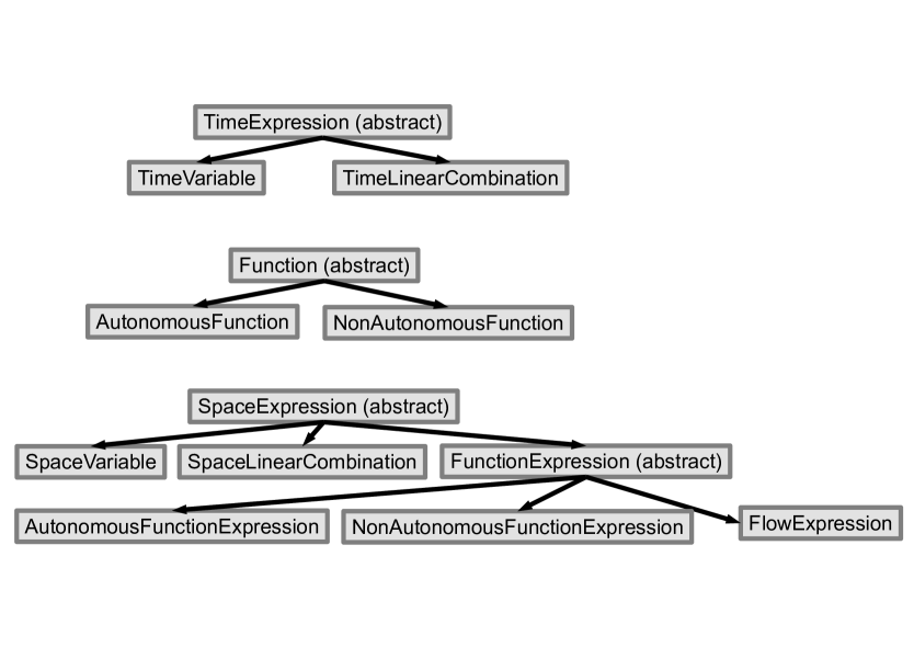
Figure 1: Data type hierarchy of Flows.jl.

Data types

The data types in the package Flows.jl and their hierarchical dependence are illustrated in Figure 1.

Objects of the abstract type TimeExpression represent a first argument $t$ in a flow expression like $\mathcal{E}_{H}(t,u)$.

Objects of type TimeVariable are generated as follows:

• In [2]: @t_vars t s r

• Out[2]: (t,s,r)

Objects of type TimeLinearCombination:

• In [3]: ex = t - 2s + 3r

• Out[3]: $3r+t-2s$

Similarly, objects of the abstract type SpaceExpression represent a second argument $u$ in a flow expression like $\mathcal{E}_{H}(t,u)$.

Objects of type SpaceVariables:

• In [4]: @x_vars u v w

• Out[4]: (u,v,w)

In order to construct objects of type AutonomousFunctionExpression or FlowExpression like $A(u)$ or $\mathcal{E}_{A}(t,u)$ we first need to declare a symbol for $A$ of type AutonomousFunction.

• In [5]: @funs A

• Out[5]: (A,)

Now we can generate objects of types AutonomousFunctionExpression and FlowExpression:

• In [6]: ex1 = A(u)

• Out[6]: $A(u)$
  

• In [7]: ex2 = E(A,t,u)

• Out[7]: $\mathcal{E}_{A}(t,u)$

Additional arguments in such expressions represent arguments for Fréchet derivatives with respect to a SpaceVariable u. Note that the order of the derivative is implicitly determined from the number of arguments.

• In [8]: ex1 = A(u,v,w)

• Out[8]: $A^{\prime\prime}(u)(v,w)$
  

• In [9]: ex2 = E(A,t,u,v)

• Out[9]: $\partial_{2}\mathcal{E}_{A}(t,u)\cdot v$

Objects of type SpaceLinearCombination can be built from such expressions:

• In [10]: ex = -2E(A,t,u,v,w)+2u+A(v,w)

• Out[10]: $-2\partial_{2}^{2}\mathcal{E}_{A}(t,u)(v,w)+2u+A^{\prime}(v)\cdot w$

Methods

differential

 
This method generates the Fréchet derivative of an expression with respect to a SpaceVariable applied to an expression.

• In [11]: ex = A(B(u)) + E(A,t,u,v)

• Out[11]: $A(B(u))+\partial_{2}\mathcal{E}_{A}(t,u)\cdot v$
  

• In [12]: differential(ex,u,B(w))

• Out[12]: $A^{\prime}(B(u))\cdot B^{\prime}(u)\cdot B(w)+\partial_{2}^{2}\mathcal{E}_{A}(t,u)(v,B(w))$

t_derivative

 
This method generates the derivative of an expression with respect to a TimeVariable.

• In [13]: ex = E(A,t-2s,u+E(B,s,v))

• Out[13]: $\mathcal{E}_{A}(t-2s,u+\mathcal{E}_{B}(s,v))$
  

• In [14]: t_derivative(ex,s)

• Out[14]: $\partial_{2}\mathcal{E}_{A}(t-2s,u+\mathcal{E}_{B}(s,v))\cdot B(\mathcal{E}_{B}(s,v))-2A(\mathcal{E}_{A}(t-2s,u+\mathcal{E}_{B}(s,v))$

expand

 
A (higher-order) Fréchet derivative is a (multi-)linear map. The method expand transforms the application of such a (multi-)linear map to a linear combination of expressions into the corresponding linear combination of (multi-)linear maps.

• In [15]: ex1 = E(A,t,u,2v+3w)

• Out[15]: $\partial_{2}\mathcal{E}_{A}(t,u)\cdot(2v+3w)$
  

• In [16]: expand(ex1)

• Out[16]: $2\partial_{2}\mathcal{E}_{A}(t,u)\cdot v+3\partial_{2}\mathcal{E}_{A}(t,u)\cdot w$
  

• In [17]: ex2 = A’’(u,v+w,v+w)

• Out[17]: $2A^{\prime\prime}(u)(v+w,v+w)$
  

• In [18]: expand(ex2)

• Out[18]: $2A^{\prime\prime}(u)(v,w)+A^{\prime\prime}(u)(v,v)+A^{\prime\prime}(u)(w,w)$

substitute

 
Different variants of substitutions are implemented. The most sophisticated one is substitution of an object of type Function by an expression. For example, this allows to define the double commutator $[A,[A,B]](u)$ by substituting $B$ in $[A,B](u)$ by $[A,B](u)$:

• In [19]: C_AB = A(u,B(u))-B(u,A(u))

• Out[19]: $A^{\prime}(u)\cdot B(u)-B^{\prime}(u)\cdot A(u)$
  

• In [20]: substitute(C_AB,B,C_AB,u)

• Out[20]: $-A^{\prime\prime}(u)(B(u),A(u))+B^{\prime}(u)\cdot A^{\prime}(u)\cdot A(u)+B^{\prime\prime}(u)(A(u),A(u))$

  $-A^{\prime}(u)\cdot B^{\prime}(u)\cdot A(u)+A^{\prime}(u)\cdot(-B^{\prime}(u)\cdot A(u)+A^{\prime}(u)\cdot B(u))$

commutator

 
This method generates expressions involving commutators $[A,B]$ and double commutators $[A,[B,C]]$.

• In [21]: ex1 = commutator(A,B,u)

• Out[21]: $A^{\prime}(u)\cdot B(u)-B^{\prime}(u)\cdot A(u)$

• In [22]: ex2 = commutator(A,B,C,u)

• Out[22]: $C^{\prime}(u)\cdot B^{\prime}(u)\cdot A(u)+C^{\prime\prime}(u)(B(u),A(u))-B^{\prime}(u)\cdot C^{\prime}(u)\cdot A(u)$

  ${}-B^{\prime\prime}(u)(C(u),A(u))+A^{\prime}(u)\cdot(B^{\prime}(u)\cdot C(u)-C^{\prime}(u)\cdot B(u))$

Example: We verify the Jacobi identity $[A,[B,C]]+[B,[C,A]]+[C,[A,B]]=0$:

• In [23]: ex3 = expand(commutator(A,B,C,u)+commutator(B,C,A,u)

  +commutator(C,A,B,u))

• Out[23]: $0$

FE2DEF, DEF2FE

 
These methods substitute expressions according to the fundamental identity

$$A(\mathcal{E}_{A}(t,u))=\partial_{2}\mathcal{E}_{A}(t,u)\cdot A(u),$$

see [4].

• In [24]: ex1 = A(E(A,t,u))

• Out[24]: $A(\mathcal{E}_{A}(t,u))$
  

• In [25]: ex2 = FE2DEF(ex1)

• Out[25]: $\partial_{2}\mathcal{E}_{A}(t,u)\cdot A(u)$
  

• In [26]: DEF2FE(ex2)

• Out[26]: $A(\mathcal{E}_{A}(t,u))$

reduce_order

 
This method constitutes the essential manipulation needed for the verification of the identities (4)–(9) in Section 2. By repeated differentiation of the fundamental identity

$$A(\mathcal{E}_{A}(t,u))-\partial_{2}\mathcal{E}_{A}(t,u)\cdot A(u)=0$$

we obtain

$$A^{\prime}(\mathcal{E}_{A}(t,u))\cdot\partial_{2}\mathcal{E}_{A}(t,u)\cdot v-\partial_{2}^{2}\mathcal{E}_{A}(t,u)(A(u),v)-\partial_{2}\mathcal{E}_{A}(t,u)\cdot A^{\prime}(u)\cdot v=0,$$

$$A^{\prime\prime}(\mathcal{E}_{A}(t,u))(\partial_{2}\mathcal{E}_{A}(t,u)\cdot v,\partial_{2}\mathcal{E}_{A}(t,u)\cdot w)+A^{\prime}(\mathcal{E}_{A}(t,u))\cdot\partial_{2}^{2}\mathcal{E}_{A}(t,u)(v,w)$$

$$\qquad-\partial_{2}^{3}\mathcal{E}_{A}(t,u)(A(u),v,w)-\partial_{2}^{2}\mathcal{E}_{A}(t,u)(A^{\prime}(u)\cdot v,w)$$

$$\qquad-\partial_{2}^{2}\mathcal{E}_{A}(t,u)(A^{\prime}(u)\cdot w,v)-\partial_{2}\mathcal{E}_{A}(t,u)\cdot A^{\prime\prime}(u)(v,w)=0,$$

and so on. The method reduce_order transforms expressions of the form of the highest order derivative in these identities by means of these very identities:

• In [27]: ex1 = E(A,t,u,A(u))

• Out[27]: $\partial_{2}\mathcal{E}_{A}(t,u)\cdot A(u)$
  

• In [28]: reduce_order(ex1)

• Out[28]: $A(\mathcal{E}_{A}(t,u))$

• In [29]: ex2 = E(A,t,u,A(u),v)

• Out[29]: $\partial_{2}^{2}\mathcal{E}_{A}(t,u)(A(u),v)$
  

• In [30]: reduce_order(ex2)

• Out[30]: $A^{\prime}(\mathcal{E}_{A}(t,u))\cdot\partial_{2}\mathcal{E}_{A}(t,u)\cdot v-\partial_{2}\mathcal{E}_{A}(t,u)\cdot A^{\prime}(u)\cdot v$
  

• In [31]: ex3 = E(A,t,u,A(u),v,w)

• Out[31]: $\partial_{2}^{3}\mathcal{E}_{A}(t,u)(A(u),v,w)$
  

• In [32]: reduce_order(ex3)

• Out[32]:

  $$\quad\,-\partial_{2}^{2}\mathcal{E}_{A}(t,u)(A^{\prime}(u)\cdot w,v)-\partial_{2}^{2}\mathcal{E}_{A}(t,u)(A^{\prime}(u)\cdot v,w)$$

  $$\quad\,-\partial_{2}\mathcal{E}_{A}(t,u)\cdot A^{\prime\prime}(u)(v,w)+A^{\prime}(\mathcal{E}_{A}(t,u))\cdot\partial_{2}^{2}\mathcal{E}_{A}(t,u)(v,w)$$

  $$\quad\,+A^{\prime\prime}(\mathcal{E}_{A}(t,u))(\partial_{2}\mathcal{E}_{A}(t,u)\cdot v,\partial_{2}\mathcal{E}_{A}(t,u)\cdot w)$$

  
  

Similarly for higher derivatives of analogous form.

4 Verification of crucial identities

We describe a Julia notebook which implements the verification of the identities (4)–(9) of Section 2.

Check (4)

We verify identity (4),

$$\partial_{t}\mathcal{S}(t,u)-H(\mathcal{S}(t,u))=\Big{[}\partial_{2}\mathcal{E}_{B}(t,v)\cdot A(v)-A(\mathcal{E}_{B}(t,v))\Big{]}_{v=\mathcal{E}_{A}(t,u)}.$$

• In [1]: using Flows
  

• In [2]: @t_vars t

• Out[2]: (t,)
  

• In [3]: @x_vars u v

• Out[3]: (u,v)
  

• In [4]: @funs A B

• Out[4]: (A,B)
  

• In [5]: E_Atu = E(A,t,u)

• Out[5]: $\mathcal{E}_{A}(t,u)$
  

• In [6]: E_Btv = E(B,t,v)

• Out[6]: $\mathcal{E}_{B}(t,v)$
  

• In [7]: Stu = E(B,t,E(A,t,u))

• Out[7]: $\mathcal{E}_{B}(t,\mathcal{E}_{A}(t,u))$
  

• In [8]: S1tv = differential(E(B,t,v),v,A(v))-A(E(B,t,v))

• Out[8]: $\partial_{2}\mathcal{E}_{B}(t,v)\cdot A(v)-A(\mathcal{E}_{B}(t,v))$
  

• In [9]: S1tu = substitute(S1tv,v,E(A,t,u))

  ex1 = S1tu

• Out[9]: $-A(\mathcal{E}_{B}(t,\mathcal{E}_{A}(t,u)))+\partial_{2}\mathcal{E}_{B}(t,\mathcal{E}_{A}(t,u))\cdot A(\mathcal{E}_{A}(t,u))$
  

• In [10]: ex2 = t_derivative(Stu,t)-(A(Stu)+B(Stu))

• Out[10]: $-A(\mathcal{E}_{B}(t,\mathcal{E}_{A}(t,u)))+\partial_{2}\mathcal{E}_{B}(t,\mathcal{E}_{A}(t,u))\cdot A(\mathcal{E}_{A}(t,u))$
  

• In [11]: ex1-ex2

• Out[11]: $0$

Check (5)

We verify identity (5),

$$\partial_{t}\tilde{\mathcal{S}}^{(1)}(t,v)=B^{\prime}(\mathcal{E}_{B}(t,v))\cdot\tilde{\mathcal{S}}^{(1)}(t,v)+[B,A](\mathcal{E}_{B}(t,v)).$$

• In [12]: ex1 = B(E(B,t,v),S1tv)+commutator(B,A,E(B,t,v))

• Out[12]: $-A^{\prime}(\mathcal{E}_{B}(t,v))\cdot B(\mathcal{E}_{B}(t,v))+B^{\prime}(\mathcal{E}_{B}(t,v))\cdot(\partial_{2}\mathcal{E}_{B}(t,v)\cdot A(v)$

  $-A(\mathcal{E}_{B}(t,v)))+B^{\prime}(\mathcal{E}_{B}(t,v))\cdot A(\mathcal{E}_{B}(t,v))$
  

• In [13]: ex2 = t_derivative(S1tv,t)

• Out[13]: $-A^{\prime}(\mathcal{E}_{B}(t,v))\cdot B(\mathcal{E}_{B}(t,v))+B^{\prime}(\mathcal{E}_{B}(t,v))\cdot\partial_{2}\mathcal{E}_{B}(t,v)\cdot A(v)$
  

• In [14]: reduce_order(expand(ex1-ex2))

• Out[14]: $0$

Check (6)

We verify identity (6),

$$\partial_{\tau}\big{(}\partial_{2}\mathcal{E}_{H}(t-\tau,\mathcal{S}(\tau,u))\cdot\,\mathcal{S}^{(1)}(\tau,u)\big{)}$$

$$=\partial_{2}\mathcal{E}_{H}(t-\tau,\mathcal{S}(\tau,u))\cdot\,\mathcal{S}^{(2)}(\tau,u)+\partial_{2}^{2}\mathcal{E}_{H}(t-\tau,\mathcal{S}(\tau,u))(\mathcal{S}^{(1)}(\tau,u),\mathcal{S}^{(1)}(\tau,u)).$$

• In [15]: @nonautonomous_funs S

• Out[15]: (S,)
  

• In [16]: @funs H

• Out[16]: (H,)
  

• In [17]: S1tu = t_derivative(S(t,u),t)-H(S(t,u))

• Out[17]: $-H(S(t,u))+\partial_{1}S(t,u)$
  

• In [18]: S2tu = t_derivative(S1tu,t)-H(S(t,u),S1tu)

• Out[18]: $-H^{\prime}(S(t,u))\cdot\partial_{1}S(t,u)+\partial_{1}^{2}S(t,u)-H^{\prime}(S(t,u))\cdot(-H(S(t,u))$

  $+\partial_{1}S(t,u))$
  

• In [19]: @t_vars T

• Out[19]: (T,)

In the following, a trailing semicolon in the input suppresses the display of the corresponding output.

• In [20]: ex1 = E(H,T-t,S(t,u),S2tu)+E(H,T-t,S(t,u),S1tu,S1tu);
  

• In [21]: ex2 = t_derivative(E(H,T-t,S(t,u),S1tu),t);
  

• In [22]: reduce_order(expand(ex1-ex2))

• Out[22]: $0$

Check (7)

We verify identity (7),

$$\partial_{t}\,\mathcal{S}^{(1)}(t,u)-H^{\prime}(\mathcal{S}(t,u))\cdot\mathcal{S}^{(1)}(t,u)$$

$$=\Big{[}\partial_{2}\tilde{\mathcal{S}}^{(1)}(t,v)\cdot A(v)-A^{\prime}(\mathcal{E}_{B}(t,v))\cdot\tilde{\mathcal{S}}^{(1)}(t,v)+[B,A](\mathcal{E}_{B}(t,v))\Big{]}_{v=\mathcal{E}_{A}(t,u)}.$$

• In [23]: S2tu = t_derivative(S1tu,t)-A(Stu,S1tu)-B(Stu,S1tu)

  ex1 = S2tu;
  

• In [24]: S2tv = (differential(S1tv,v,A(v))-A(E(B,t,v),S1tv)

  +commutator(B,A,E(B,t,v)))

  ex2 = substitute(S2tv,v,E(A,t,u));
  

• In [25]: expand(ex1-ex2)

• Out[25]: $0$

Check (8)

We verify identity (8),

$$\partial_{t}\tilde{\mathcal{S}}^{(2)}(t,v) =B^{\prime}(\mathcal{E}_{B}(t,v))\cdot\tilde{\mathcal{S}}^{(2)}(t,v)$$

$$\quad{}+B^{\prime\prime}(\mathcal{E}_{B}(t,v))(\tilde{\mathcal{S}}^{(1)}(t,v),\tilde{\mathcal{S}}^{(1)}(t,v))$$

$$\quad{}-[B,[B,A]](\mathcal{E}_{B}(t,v))-[A,[B,A]](\mathcal{E}_{B}(t,v))$$

$$\quad{}+2[B,A]^{\prime}(\mathcal{E}_{B}(t,v))\cdot\tilde{\mathcal{S}}^{(1)}(t,v).$$

• In [26]: ex1 = (B(E(B,t,v),S2tv) + B(E(B,t,v),S1tv,S1tv)

  -commutator(B,B,A,E(B,t,v))

  -commutator(A,B,A,E(B,t,v))

  +2*substitute(differential

  (commutator(B,A,w),w,S1tv),w,E(B,t,v)));
  

• In [27]: ex2 = t_derivative(S2tv,t);
  

• In [28]: expand(ex1-ex2)

• Out[28]: $0$

Check (9)

We verify identity (9),

$$\partial_{\tau}\Big{(}\partial_{2}\mathcal{E}_{H}(t-\tau,\mathcal{S}(\tau,u))\cdot\partial_{2}\mathcal{E}_{B}(\tau,\mathcal{E}_{A}(\tau,u))\cdot[B,A](\mathcal{E}_{A}(\tau,u))\Big{)}=$$

$$\qquad\Big{[}\partial_{2}\mathcal{E}_{H}(t-\tau,\mathcal{E}_{B}(\tau,v))\cdot\partial_{2}\mathcal{E}_{B}(\tau,v)\cdot[[B,A],A](v)$$

$$\qquad\qquad{}+\partial_{2}\mathcal{E}_{H}(t-\tau,\mathcal{E}_{B}(\tau,v))\cdot\partial_{2}\tilde{\mathcal{S}}^{(1)}(\tau,v)\cdot[B,A](v)$$

$$\qquad\qquad{}+\partial_{2}^{2}\mathcal{E}_{H}(t-\tau,\mathcal{E}_{B}(\tau,v))\big{(}\tilde{\mathcal{S}}^{(1)}(\tau,v),\partial_{2}\mathcal{E}_{B}(\tau,v)\cdot[B,A](v)\big{)}\Big{]}_{v=\mathcal{E}_{A}(t,u)}.$$

• In [29]: ex1 = t_derivative(E(H,T-t,Stu,E(B,t,E(A,t,u),

  commutator(B,A,E(A,t,u)))),t);

• In [30]: ex2 = (substitute(-E(H,T-t,E(B,t,v),E(B,t,v,

  commutator(A,B,A,v)))+E(H,T-t,E(B,t,v),

  differential(S1tv,v,commutator(B,A,v)))

  +E(H,T-t,E(B,t,v),S1tv,E(B,t,v,

  commutator(B,A,v))),v,E(A,t,u)));
  

• In [31]: diff = ex1-ex2

  diff = FE2DEF(diff)

  diff = substitute(diff,H,A(v)+B(v),v)

  diff = expand(reduce_order(diff))

• Out[31]: $0$

5 Elementary differentials

To further demonstrate the functionality and correctness of our package, we consider the elementary differentials obtained by repeated differentiation of a differential equation,

$$y^{\prime}(t) =F(y(t)),$$

$$y^{\prime\prime}(t) =F^{\prime}(y(t))\cdot F(y(t)),$$

$$y^{\prime\prime\prime}(t) =F^{\prime\prime}(y(t))(F(y(t),F(y(t))+F^{\prime}(y(t))\cdot F^{\prime}(y(t))\cdot F(y(t)),$$

$$~{}~{}\vdots$$

The number of terms in these expressions are available from the literature, see [6, Table 2.1] or [3]. The following notebook generates the elementary differentials and counts their number:

• In [1]: using Flows
  

• In [2]: @t_vars t;

  @x_vars u;

  @funs F;
  

• In [3]: ex = E(F,t,u)

• Out[3]: $\mathcal{E}_{F}(t,u)$
  

• In [4]: ex = t_derivative(ex,t)

• Out[4]: $F(\mathcal{E}_{F}(t,u))$
  

• In [5]: ex = t_derivative(ex,t)

• Out[5]: $\;F^{\prime}(\mathcal{E}_{F}(t,u))\cdot F(\mathcal{E}_{F}(t,u))$
  

• In [6]: ex = t_derivative(ex,t)

• Out[6]:

  $$F^{\prime}(\mathcal{E}_{F}(t,u))\cdot F^{\prime}(\mathcal{E}_{F}(t,u))\cdot F(\mathcal{E}_{F}(t,u))$$

  $$+F^{\prime\prime}(\mathcal{E}_{F}(t,u))(F(\mathcal{E}_{F}(t,u)),F(\mathcal{E}_{F}(t,u)))\qquad\qquad\qquad~{}~{}$$

• In [7]: ex = t_derivative(ex,t)

• Out[7]:

  $$3F^{\prime\prime}(\mathcal{E}_{F}(t,u))(F^{\prime}(\mathcal{E}_{F}(t,u))\cdot F(\mathcal{E}_{F}(t,u)),F(\mathcal{E}_{F}(t,u)))\quad\,\,\,\,$$

  $$+F^{\prime\prime\prime}(\mathcal{E}_{F}(t,u))(F(\mathcal{E}_{F}(t,u)),F(\mathcal{E}_{F}(t,u)),F(\mathcal{E}_{F}(t,u)))$$

  $$+F^{\prime}(\mathcal{E}_{F}(t,u))\cdot(F^{\prime}(\mathcal{E}_{F}(t,u))\cdot F^{\prime}(\mathcal{E}_{F}(t,u))\cdot F(\mathcal{E}_{F}(t,u))$$

  $$+F^{\prime\prime}(\mathcal{E}_{F}(t,u))(F(\mathcal{E}_{F}(t,u)),F(\mathcal{E}_{F}(t,u))))$$

  
  

This is not yet fully expanded. It is a linear combination consisting of 3 terms:

• In [8]: length(ex.terms)

• Out[8]: 3

If we expand it, we obtain a linear combination of 4 terms, corresponding to the 4 elementary differentials (Butcher trees) of order 4:

• In [9]: ex = expand(ex)

• Out[9]:

  $$3F^{\prime\prime}(\mathcal{E}_{F}(t,u))(F^{\prime}(\mathcal{E}_{F}(t,u))\cdot F(\mathcal{E}_{F}(t,u)),F(\mathcal{E}_{F}(t,u)))$$

  $$+F^{\prime}(\mathcal{E}_{F}(t,u))\cdot F^{\prime}(\mathcal{E}_{F}(t,u))\cdot F^{\prime}(\mathcal{E}_{F}(t,u))\cdot F(\mathcal{E}_{F}(t,u))$$

  $$+F^{\prime\prime\prime}(\mathcal{E}_{F}(t,u))(F(\mathcal{E}_{F}(t,u)),F(\mathcal{E}_{F}(t,u)),F(\mathcal{E}_{F}(t,u)))$$

  $$+F^{\prime}(\mathcal{E}_{F}(t,u))\cdot F^{\prime\prime}(\mathcal{E}_{F}(t,u))(F(\mathcal{E}_{F}(t,u)),F(\mathcal{E}_{F}(t,u)))$$

  
  

• In [10]: length(ex.terms)

• Out[10]: 4
  

• In [11]: ex = expand(t_derivative(ex,t));
  

• In [12]: length(ex.terms)

• Out[12]: 9
  

• In [13]: ex = expand(t_derivative(ex,t));
  

• In [14]: length(ex.terms)

• Out[14]: 20
  

• In [15]: ex = expand(t_derivative(ex,t));
  

• In [16]: length(ex.terms)

• Out[16]: 48

   In [17]: ex = E(F,t,u)
            ex = expand(t_derivative(ex,t))
            println("order\t#terms")
            println("---------------")
            println(1,"\t",1)
            ex = expand(t_derivative(ex,t))
            println(2,"\t",1)
            for k=3:16
                ex = expand(t_derivative(ex,t))
                println(k,"\t",length(ex.terms))
            end

     order   #terms
     ---------------
     1       1
     2       1
     3       2
     4       4
     5       9
     6       20
     7       48
     8       115
     9       286
     10      719
     11      1842
     12      4766
     13      12486
     14      32973
     15      87811
     16      235381

6 Acknowledgments

This work was supported in part by the projects P24157-N13 of the Austrian Science Fund (FWF) and MA14-002 of the Vienna Science and Technology Fund (WWTF).

References

• [1] http://julialang.org
• [2] https://github.com/HaraldHofstaetter/Flows.jl
• [3] The On-line Encyclopedia of Integer Sequences. https://oeis.org/A000081
• [4] Auzinger, W., Hofstätter, H., Koch, O., Thalhammer, M.: Defect-based local error estimators for splitting methods, with application to Schrödinger equations, Part III: The nonlinear case. J. Comput. Appl. Math. 273, 182–204 (2014)
• [5] Hairer, E., Lubich, C., Wanner, G.: Geometric Numerical Integration. Springer-Verlag, Berlin–Heidelberg–New York (2002)
• [6] Hairer, E., Nørsett, S., Wanner, G.: Solving Ordinary Differential Equations I, 2nd edition. Springer-Verlag, Berlin–Heidelberg–New York (1993)