Cryptographic quantum bound on nonlocality

Abstract

Information causality states that the information obtainable by a receiver cannot be greater than the communication bits from a sender, even if they utilize no-signaling resources. This physical principle successfully explains some boundaries between quantum and postquantum nonlocal correlations, where the obtainable information reaches the maximum limit. We show that no-signaling resources of pure partially entangled states produce randomness (or noise) in the communication bits, and achievement of the maximum limit is impossible, i.e., the information causality principle is insufficient for the full identification of the quantum boundaries already for bipartite settings. The nonlocality inequalities such as so-called the Tsirelson inequality are extended to show how such randomness affects the strength of nonlocal correlations. As a result, a relation followed by most of quantum correlations in the simplest Bell scenario is revealed. The extended inequalities reflect the cryptographic principle such that a completely scrambled message cannot carry information.

I Introduction

It was shown by Bell that the nonlocal correlations predicted by quantum mechanics are inconsistent with local realism Bell (1964). The nonlocal correlations do not contradict the no-signaling principle that prohibits instantaneous communication. However, it was found that the set of quantum correlations is strictly smaller than the set of no-signaling correlations Cirel’son (1980); Popescu and Rohrlich (1994). Concretely, a particular type of the Bell inequality, the Clauser-Horne-Shimony-Holt (CHSH) inequality Clauser et al. (1969), was shown to be violated up to $4$ in general no-signaling correlations Popescu and Rohrlich (1994), while from the Tsirelson inequality Cirel’son (1980) the violation is bounded by $2\sqrt{2}$ in quantum correlations. Since then, many efforts have been made to search for a simple physical principle to close this discrepancy. See Brunner et al. (2014); Popescu (2014); Oas and de Barros (2016) for a good review.

Information causality (IC) Pawłowski et al. (2009) is such a physical principle. Consider two remote parties, Alice and Bob, who share no-signaling nonlocal resources such as entangled states. When Alice sends a message to Bob, IC states that the total information obtainable by Bob cannot be greater than the number of the message bits even if they utilize the no-signaling resources Pawłowski et al. (2009). A powerful necessary condition for respecting the IC principle was derived by considering an explicit communication protocol Pawłowski et al. (2009). The condition, called the IC inequality hereafter, successfully explains the Tsirelson inequality, and even explains some curved boundaries between quantum and postquantum correlations Pawłowski et al. (2009); Allcock et al. (2009). At those quantum boundaries, the protocol achieves the maximum limit of the obtainable information (the number of the message bits). It is then expected that, for every quantum boundary, there exists a protocol for which the maximum limit is achieved.

Apart from searching for physical principles, the identification of the quantum boundaries is originally a difficult problem. Indeed, the analytical necessary and sufficient criterion for the identification has not been given yet even in the simplest Bell scenario, although the Tsirelson-Landau-Masanes (TLM) criterion Tsirelson (1987); Landau (1988); Masanes is known for a case of unbiased marginal probabilities (explain later).

In this paper, we show that pure partially entangled states, which were shown to give rise to boundary correlations Liang et al. (2011); Acín et al. (2012); Ramanathan et al. ; Zhen et al. (2016), produce randomness in the message, and achievement of the maximum limit is impossible no matter what protocol is executed. Hence, the IC principle is insufficient for the full identification of the quantum boundaries already for bipartite settings (similar results have been obtained in multipartite settings Gallego et al. (2011); Yang et al. (2012)). We extend the nonlocality inequalities to include the effects of the randomness. As a result, a relation followed by most of quantum correlations, including both cases of unbiased and biased marginals, is revealed. Moreover, we show that the derived inequalities reflect the cryptographic principle such that a completely scrambled message cannot carry information Shannon (1949). The inequalities reflecting the cryptographic principle contain a quantity defined in quantum mechanics, and the principle cannot immediately exclude postquantum correlations by itself, but tells us a way to determine the quantum boundaries. Note that a similar principle for a different type of randomness was considered in Carmi and Moskovich .

Let us here show a simple example to clarify what we mean by randomness. Consider the simplest Bell scenario, where Alice is given a random bit $x$ and performs the measurement on the partially entangled state $\sqrt{2/3}|00\rangle\!+\!\sqrt{1/3}|11\rangle$ in the basis $|0\rangle/|1\rangle$ for $x\!=\!0$ or $(|0\rangle\pm|1\rangle)/\sqrt{2}$ for $x\!=\!1$, and obtains the outcome $a$. Suppose that Bob somehow knows that $x$ was 1. However, he still cannot determine the value of $a$ completely, because his local state is $\sqrt{2/3}|0\rangle\!+\!\sqrt{1/3}|1\rangle$ for $a\!=\!0$ or $\sqrt{2/3}|0\rangle\!-\!\sqrt{1/3}|1\rangle$ for $a\!=\!1$, which are nonorthogonal. This means that $a$ has some uncertainty indeterminable for Bob, and the uncertainty acts as randomness (or noise) if $a$ is used for the transmission of the information of $x$ (the details are discussed in Sec. IV). As a result, the obtainable information of Bob is reduced. This affects the quantum bound of the CHSH inequality, and the violation is reduced to $2\sqrt{17/9}$ [see Eq. (3) below] from the maximum value of $2\sqrt{2}$.

This paper is organized as follows. In Sec. II, we extend the Tsirelson inequality, the IC inequality, and the Landau inequality (of the TLM criterion) by including the state-dependent quantity measuring the orthogonality between Bob’s local states, because nonorthogonality is key to the randomness as in the above example. In Sec. III, we discuss the tightness of the derived Landau-type inequality, and show that the inequality is widely saturated for both boundary and non-boundary correlations even in the case of biased marginals. We then discuss the information theoretical aspects of the derived IC-type inequality in Sec. IV, where the connection to the cryptographic principle and the insufficiency of the IC principle are shown. In Sec. V, we show an example of how to determine the quantum boundaries under the cryptographic principle. A summary is given in Sec. VI.

II Bounds on nonlocality

To begin with, let us derive the inequalities discussed in this paper. The derivation is surprisingly simple. Consider the simplest Bell scenario, where Alice and Bob share a quantum state, Alice (Bob) performs a measurement depending on a given bit $x$ ($y$) to obtain the outcome bit $a$ ($b$). Their shared state is a pure or mixed state denoted by $\rho$. We use the shorthand notation $\langle\cdots\rangle$ for $\hbox{tr}\rho\cdots$. Without loss of generality, we can assume that they perform projective measurements, because no assumption is made about the system dimension. The observable of Alice (Bob), denoted by $A_{x}$ ($B_{y}$), then satisfies $A_{x}^{2}\!=\!B_{x}^{2}\!=\!I$ with $I$ being the identity operator. The projector of the measurement for Alice’s outcome $a$ is given by $P_{a|x}\!=\!(I+(-1)^{a}A_{x})/2$, and for Bob’s outcome $b$ by $Q_{b|y}\!=\!(I+(-1)^{b}B_{y})/2$. Let us then consider the weighted CHSH expression Lowson et al. (2010) of the form:

$${\cal B}=\sum_{y}t_{y}s_{x}(-1)^{xy}\langle A_{x}\!\otimes\!B_{y}\rangle=\sum_{y}t_{y}E_{y},$$ (1)

where $t_{y}$ and $s_{x}$ are real non-negative parameters, and $E_{y}\!\equiv\!s_{0}\langle A_{0}\!\otimes\!B_{y}\rangle+s_{1}(-1)^{y}\langle A_{1}\!\otimes\!B_{y}\rangle$ is introduced for later convenience. If we define $X_{x}\!\equiv\!t_{0}B_{0}\!+\!(-1)^{x}t_{1}B_{1}$, it can be seen that $X^{2}_{0}\!+\!X^{2}_{1}\!=\!2(t^{2}_{0}\!+\!t^{2}_{1})I$, and we obtain the Tsirelson-type inequality as follows:

$${\cal B} \!\!\!=\!\!\! \sum_{x}s_{x}\sqrt{\langle I\!\otimes\!X^{2}_{x}\rangle}\frac{\langle A_{x}\!\otimes\!X_{x}\rangle}{\sqrt{\langle I\!\otimes\!X^{2}_{x}\rangle}}\leq\sum_{x}s_{x}\sqrt{\langle I\!\otimes\!X^{2}_{x}\rangle}\tilde{D}_{x}$$ (3)

$$\leq\sqrt{2(t_{0}^{2}+t_{1}^{2})(s_{0}^{2}\tilde{D}^{2}_{0}+s_{1}^{2}\tilde{D}^{2}_{1})},$$

where we used $\sum_{x}\langle I\!\otimes\!X_{x}^{2}\rangle\!=\!2(t^{2}_{0}\!+\!t^{2}_{1})$ as a constraint in the last inequality. The quantity $\tilde{D}_{x}$ is defined by

$$\tilde{D}_{x}\equiv\max_{X}\frac{\langle A_{x}\!\otimes\!X\rangle}{\sqrt{\langle I\!\otimes\!X^{2}\rangle}}=\max_{X}\frac{\hbox{tr}X(\rho_{0|x}-\rho_{1|x})}{\sqrt{\hbox{tr}X^{2}(\rho_{0|x}+\rho_{1|x})}},$$ (4)

where the maximization is taken over all Hermitian operators $X$, and $\rho_{a|x}\!=\!\hbox{tr}_{A}(P_{a|x}\!\otimes\!I)\rho$ is Bob’s subnormalized state when Alice is given $x$ and her outcome is $a$. The quantity $\tilde{D}_{x}$ is quite analogous to the generalized trace distance $\bar{D}_{x}=\hbox{tr}|\rho_{0|x}-\rho_{1|x}|$ (the extension of the trace distance to subnormalized states). Indeed, both agree with each other for the case of pure states. For the other general cases, $\tilde{D}_{x}\!\geq\!\bar{D}_{x}$. See Appendix A for the proofs of those properties. It is obvious from the definition of Eq. (4) that $\tilde{D}_{x}\!\leq\!1$, because it is the inner product of the two normalized states $(A_{x}\!\otimes\!I)|\psi\rangle$ and $(I\!\otimes\!X)|\psi\rangle/\sqrt{\langle\psi|I\!\otimes\!X^{2}|\psi\rangle}$ (consider a purification $|\psi\rangle$ if $\rho$ is a mixed state), and the inner product is ensured to be real Tsirelson (1987); Vértesi and Pál (2008). Note that a different type of quantum bounds using the trace distance was shown in Liang and Doherty (2007). Since the envelope of the boundaries of Eq. (3) in the $(E_{0},E_{1})$-space is a quarter-circle, considering the symmetry with respect to $B_{y}\!\rightarrow\!-B_{y}$ and putting $s_{0}\!=\!s_{1}\!=\!1/2$, we have the IC-type inequality:

$$E^{2}_{0}+E^{2}_{1}\leq\frac{\tilde{D}^{2}_{0}+\tilde{D}^{2}_{1}}{2}.$$ (5)

Note that $E_{0}$ and $E_{1}$ coincides with $E_{\rm I}$ and $E_{\rm II}$ in Pawłowski et al. (2009), respectively.

In the same technique as above, a tighter quantum bound is obtained by considering more general weight parameters as follows:

$$\sum_{xy}s_{x}u_{xy}(-1)^{xy}\langle A_{x}\otimes B_{y}\rangle\leq\big{[}\sum_{xy}u^{2}_{xy}\big{]}^{\frac{1}{2}}\big{[}\sum_{x}s^{2}_{x}\tilde{D}^{2}_{x}\big{]}^{\frac{1}{2}},$$ (6)

where $s_{x}$ and $u_{xy}$ are real parameters satisfying $u_{00}u_{01}\!=\!u_{10}u_{11}$. When $\tilde{D}_{0},\tilde{D}_{1}\!>\!0$, the necessary and sufficient condition for the above inequality is given by

$$\left|\tilde{C}_{00}\tilde{C}_{01}-\tilde{C}_{10}\tilde{C}_{11}\right| \leq (1-\tilde{C}^{2}_{00})^{\frac{1}{2}}(1-\tilde{C}^{2}_{01})^{\frac{1}{2}}$$ (7)

$$+ (1-\tilde{C}^{2}_{10})^{\frac{1}{2}}(1-\tilde{C}^{2}_{11})^{\frac{1}{2}},$$ (8)

where $\tilde{C}_{xy}\!\equiv\!\langle A_{x}\otimes B_{y}\rangle/\tilde{D}_{x}\!\equiv\!C_{xy}/\tilde{D}_{x}$. The derivation is given in Appendix B. This is an extension of the Landau inequality Landau (1988). The Landau inequality is a representation of the TLM criterion, and hence is necessary and sufficient so that a given set of the conditional probabilities $\{p(ab|xy)\}$ (or a given set of $\{C_{xy}\}$) is quantum realizable in the case of unbiased marginals such that $p(a|x)\!=\!p(b|y)\!=\!1/2$. It is known that the Navascués-Pironio-Acín (NPA) inequality Navascués et al. (2007, 2008) gives a tighter bound than the Landau inequality for the case of biased marginals. It is also possible to extend the NPA inequality to include $\tilde{D}_{x}$ as shown in Appendix B.

The above inequalities all represent the effects of the nonorthogonality between Bob’s local states for $a\!=\!0$ and 1. Indeed, when $\rho_{0|x}$ and $\rho_{1|x}$ are orthogonal for both $x=0$ and $1$, we have $\tilde{D}_{0}\!=\!\tilde{D}_{1}\!=\!1$, and those reproduce the inequalities known so far. Note that $\tilde{D}_{x}\!=\!1$ if and only if $\bar{D}_{x}\!=\!1$ (see Appendix A) and so also in the case of $\hbox{tr}\rho_{0|x}\!=\!0$ or $\hbox{tr}\rho_{1|x}\!=\!0$. This is included in the orthogonal case throughout this paper.

III Tightness of bounds

The inequalities derived in Sec. II must hold for all physical realizations (by projective measurements). A nonlocal correlation is generally identified by the set of conditional probabilities $\{p(ab|xy)\}$, and the left-hand side of e.g., Eq. (6) is determined by $\{p(ab|xy)\}$ only (for a fixed weight). On the other hand, the right-hand side is monotonically increasing with respect to $\tilde{D}_{x}$. It is then found that, if a set $\{p(ab|xy)\}$ saturates the Landau inequality [i.e., the equality of Eq. (6) holds with $\tilde{D}_{0}\!=\!\tilde{D}_{1}\!=\!1$ by appropriately chosen weight parameters], the realization that produces the same $\{p(ab|xy)\}$ but with $\tilde{D}_{x}\!<\!1$ is not allowed. Namely, we have the following:

Lemma 1. For every correlation that saturates the Landau inequality, there is no realization such that Bob’s subnormalized states $\rho_{0|x}$ and $\rho_{1|x}$ are nonorthogonal. The same holds for Alice’s states.

Note that this is the case of the NPA inequality by Eq. (41). Note further that Lemma 1 is consistent with the fact that the nonclassical boundary correlations with unbiased marginals are all used for the self-testing of the maximally entangled state of two qubits, i.e., solely realized by the maximally entangled state Wang et al. (2016), because every boundary correlation with unbiased marginals is given by the saturation of the Landau inequality.

In the case of the Landau-type inequality Eq. (8) that includes $\tilde{D}_{x}$, the saturation does not necessarily imply that the correlation is located at a boundary. Rather, the inequality is widely saturated even for non-boundary correlations. To see this, let us consider the completely random correlation $\mathbf{I}$ given by $p(ab|xy)=1/4$ ($\forall a,b,x,y$), which is realized by the maximally mixed state of two qubits $\rho_{AB}\!=\!\frac{1}{4}I_{A}\!\otimes\!I_{B}$, where $C_{xy}\!=\!0$ and $\tilde{D}_{x}\!=\!0$. Then, if Eq. (8) is saturated for a correlation $\mathbf{p}$ by some realization, it is also done for $\mathbf{q}$ of the form

$$\mathbf{q}\!=\!\lambda\mathbf{p}+(1-\lambda)\mathbf{I},$$ (9)

where $0\!\leq\!\lambda\!\leq\!1$. This is because, when $\mathbf{p}$ is realized by $\rho^{\mathbf{p}}_{AB}$, $\mathbf{q}$ is realized by the shared state of

$$\rho^{\mathbf{p}}_{AB}\otimes({\textstyle\frac{1}{4}}I_{A}\otimes I_{B})\otimes\big{[}\lambda|00\rangle\langle 00|+(1-\lambda)|11\rangle\langle 11|\big{]}_{AB}$$ (10)

such that Alice and Bob switch their measured states (and the corresponding measurements) between $\rho^{\mathbf{p}}_{AB}$ and $\frac{1}{4}(I_{A}\!\otimes\!I_{B})$ according to the shared randomness produced by $\lambda|00\rangle\langle 00|\!+\!(1\!-\!\lambda)|11\rangle\langle 11|$, and it is found from the closed form of $\tilde{D}_{x}$ (see Appendix A) that $\tilde{D}_{x}$ for $\mathbf{q}$ and $\mathbf{p}$ are related through $\tilde{D}^{\mathbf{q}}_{x}\!=\!\lambda\tilde{D}^{\mathbf{p}}_{x}\!+\!(1-\lambda)\tilde{D}^{\mathbf{I}}_{x}\!=\!\lambda\tilde{D}^{\mathbf{p}}_{x}$, and hence $\tilde{C}^{\mathbf{q}}_{xy}\!=\!\tilde{C}^{\mathbf{p}}_{xy}$ holds. This implies that, if Eq. (8) is saturated for every boundary of the set of quantum correlations, the inequality is saturated for all correlations inside the set. This is indeed the case of unbiased marginals, because the inequality is saturated for every boundary with $\tilde{D}_{0}\!=\!\tilde{D}_{1}\!=\!1$, and we obtain the following:

Lemma 2. For every correlation with unbiased marginals, there always exists a realization such that the equality holds in Eq. (8).

An important observation is that the inequality is saturated even for the case of biased marginals. A two-qubit realization to give the maximal violation of the Bell expression $\beta\langle A_{0}\rangle+\alpha\langle A_{0}B_{0}\rangle+\alpha\langle A_{0}B_{1}\rangle+\langle A_{1}B_{0}\rangle-\langle A_{1}B_{1}\rangle$ was shown in Acín et al. (2012), where the partially entangled state $|\psi\rangle=\cos\theta|00\rangle+\sin\theta|11\rangle$ produces the boundary correlations with biased marginals. In this realization, we have $\tilde{D}_{0}\!=\!1$ and $\tilde{D}_{1}\!=\!\sin 2\theta$ irrespective of $\alpha$, $\tilde{C}_{00}\!=\!\tilde{C}_{01}\!=\!\frac{\alpha}{\sqrt{\sin^{2}2\theta+\alpha^{2}}}$, $\tilde{C}_{10}\!=\!-\tilde{C}_{11}\!=\!\frac{\sin 2\theta}{\sqrt{\sin^{2}2\theta+\alpha^{2}}}$, and Eq. (8) is saturated for a whole range of $\alpha$ and $\sin 2\theta$.

It is known that any extremal nonclassical correlation in the simplest Bell scenario has a two-qubit realization, where projective measurements of rank 1 are performed on a pure entangled state Masanes (2006). For such extremal realizations, by applying appropriate local unitary transformations, Alice and Bob’s observables are written as

$$A_{x}=\cos\theta^{A}_{x}\sigma_{1}+\sin\theta^{A}_{x}\sigma_{3},\hbox{~{}}B_{y}=\cos\theta^{B}_{y}\sigma_{1}+\sin\theta^{B}_{y}\sigma_{3},$$ (11)

where $(\sigma_{1},\sigma_{3},\sigma_{3})$ are the Pauli matrices. Moreover, $\rho\!=\!|\psi\rangle\langle\psi|$ is chosen to be real symmetric, and let us express

$$\!\!\!\!\!\!\!\!\hbox{tr}_{A}(A_{x}\!\otimes\!I)|\psi\rangle\langle\psi| \!\!=\!\! \alpha^{B}_{x}I+\beta^{B}_{x}(\cos\phi^{B}_{x}\sigma_{1}+\sin\phi^{B}_{x}\sigma_{3}),$$ (12)

$$\!\!\!\!\!\!\!\!\hbox{tr}_{B}(I\!\otimes\!B_{y})|\psi\rangle\langle\psi| \!\!=\!\! \alpha^{A}_{y}I+\beta^{A}_{y}(\cos\phi^{A}_{y}\sigma_{1}+\sin\phi^{A}_{y}\sigma_{3}).$$ (13)

As shown in Appendix C, the necessary and sufficient condition for the saturation of Eq. (8) is given by

$$\sin(\phi^{B}_{0}-\theta^{B}_{0})\sin(\phi^{B}_{0}-\theta^{B}_{1})\sin(\phi^{B}_{1}-\theta^{B}_{0})\sin(\phi^{B}_{1}-\theta^{B}_{1})\leq 0.$$ (14)

Similarly, for the counterpart inequality on Alice’s side,

$$\sin(\phi^{A}_{0}-\theta^{A}_{0})\sin(\phi^{A}_{0}-\theta^{A}_{1})\sin(\phi^{A}_{1}-\theta^{A}_{0})\sin(\phi^{A}_{1}-\theta^{A}_{1})\leq 0.$$ (15)

We have performed the Monte Carlo calculations, where a two-qubit realization to give the maximal violation of a randomly generated Bell expression is obtained. The numerical results suggest that Eq. (14) and (15) are simultaneously satisfied for all nonclassical extremal correlations, and hence support the following conjecture:

Conjecture 1. For every extremal correlation, there always exists a realization such that the equality holds in Eq. (8) and in the counterpart inequality on Alice’s side.

In this way, most of correlations including the case of biased marginals appear to obey a simple and unified rule, which is revealed by considering the nonorthogonality between local states. Note that, when the real symmetric $\rho$ is maximally entangled, Eq. (14) and (15), which specify a geometric relation between angles (see Wang et al. (2016)), are necessary and sufficient for the extremality of the generated correlation with unbiased marginals. When the real symmetric $\rho$ is chosen to be pure and partially entangled, do those provide a simple necessary and sufficient condition for the extremality also in the case of biased marginals? This is an intriguing open problem.

IV Information theoretical aspects

To discuss the information theoretical aspects of the IC-type inequality Eq. (5), let us introduce a communication protocol. A nonlocal game known as the inner product game has been studied in connection to communication complexity Buhrman et al. (2010); van Dam (2013). The protocol we consider is its communication version shown in Fig. 1, where Alice and Bob is given a random $n$-bit string $\vec{x}\!=\!(x_{1},\cdots,x_{n})$ and $\vec{y}\!=\!(y_{1},\cdots,y_{n})$ generated with the probability $s_{\vec{x}}$ and $t_{\vec{y}}$, respectively. Alice (Bob) outputs a bit $a_{p}$ ($b_{p}$) utilizing shared quantum states, and she sends the message $m$ to Bob that is $a_{p}$ scrambled by an independent random bit $r$ such as $m=a_{p}\oplus r$. The purpose of this protocol is that Bob obtains the value of $(\vec{x}\cdot\vec{y})\oplus r$, where $\vec{x}\cdot\vec{y}\!=\!\sum_{i}x_{i}y_{i}\mod 2$. The task is nontrivial even for $\vec{y}=(0,\cdots,0)$ due to the scrambling by $r$. A more important role of $r$ becomes clear later. Let $A_{\vec{x}}$ ($B_{\vec{y}}$) be the observable of Alice (Bob) to obtain $a_{p}$ ($b_{p}$), and the projector of Alice (Bob) be $P_{a_{p}|\vec{x}}$ ($Q_{b_{p}|\vec{y}}$). Then, Bob’s success probability for a given $\vec{y}$ averaged over $\vec{x}$ is

$$p_{\vec{y}} = \sum_{\vec{x}}s_{\vec{x}}\sum_{a_{p}b_{p}}\langle P_{a_{p}|\vec{x}}\otimes Q_{b_{p}|\vec{y}}\rangle\delta_{\vec{x}\cdot\vec{y}=a_{p}\oplus b_{p}}$$ (16)

$$= \frac{1}{2}\big{(}1+\sum_{\vec{x}}s_{\vec{x}}\langle A_{\vec{x}}\otimes(-1)^{\vec{x}\cdot\vec{y}}B_{\vec{y}}\rangle\big{)}.$$ (17)

Concerning the quantum bound of the bias $E_{\vec{y}}\!\equiv\!2p_{\vec{y}}\!-\!1$, the discussion runs in parallel with Sec. II. Indeed, $\sum_{\vec{x}}X_{\vec{x}}^{2}\!=\!2^{n}\sum_{\vec{y}}t_{\vec{y}}^{2}I$ holds for $X_{\vec{x}}\!\equiv\!\sum_{\vec{y}}t_{\vec{y}}(-1)^{\vec{x}\cdot\vec{y}}B_{\vec{y}}$, hence $\sum_{\vec{y}}t_{\vec{y}}E_{\vec{y}}\!\leq\!(2^{n}\sum_{\vec{x}\vec{y}}t_{\vec{y}}^{2}s_{\vec{x}}^{2}\tilde{D}^{2}_{\vec{x}})^{\frac{1}{2}}$, and we have $\sum_{\vec{y}}E^{2}_{\vec{y}}\!\leq\!2^{n}\sum_{\vec{x}}s_{\vec{x}}^{2}\tilde{D}^{2}_{\vec{x}}$. Let us now assume that Alice and Bob utilize the $n$ identical “quantum boxes”, each of which accepts inputs $(x,y)$ and produces outputs $(a,b)$ according to $\{p(ab|xy)\}$, and assume that $a_{p}$ ($b_{p}$) is the parity bit of Alice’s (Bob’s) outputs from the $n$ boxes as shown in Fig. 1. Under those assumptions, $B_{\vec{y}}$ must have a tensor product form such as $B_{\vec{y}}\!=\!B_{y_{1}}\otimes B_{y_{2}}\otimes\cdots$, which implies that the maximization operator $X$ in $\tilde{D}_{\vec{x}}$ also has a tensor product form. It is then found that

$$\sum_{\vec{y}}E^{2}_{\vec{y}}\leq\big{(}\frac{\tilde{D}^{2}_{0}+\tilde{D}^{2}_{1}}{2}\big{)}^{n}$$ (18)

must hold in this protocol for $s_{\vec{x}}\!=\!1/2^{n}$, whose right-hand side is the $n$-th power of the right-hand side of Eq. (5).

In the general setting of communication, where Alice is given $\vec{x}$ and sends the bit string $\vec{m}$ to Bob as a message, the information obtainable by Bob is characterized by the mutual information $I(\vec{x}\!:\!\vec{m}\rho_{B})$, where $\rho_{B}$ is the state of Bob’s half of no-signaling resources. Using the no-signaling condition and the information-theoretical relations respected by quantum mechanics, it was shown that Pawłowski et al. (2009); Dahlsten et al. (2012); Al-Safi and Short (2011)

$$I(\vec{x}:\vec{m}\rho_{B}) = I(\vec{m}:\vec{x}\rho_{B})-I(\vec{m}:\rho_{B})$$ (19)

$$\leq H(\vec{m})-H(\vec{m}|\vec{x}\rho_{B})\leq H(\vec{m}).$$ (20)

Since the entropy $H(\vec{m})$ cannot exceed the number of bits in $\vec{m}$, the IC principle is derived. The left-hand side of Eq. (18), where the $2^{n}$ variables Bob tries to obtain are pair-wise independent Pawłowski and Winter (2012); Al-Safi and Short (2011); Bavarian and Shor (2015), generally corresponds to the term $I(\vec{x}\!:\!\vec{m}\rho_{B})$. To investigate the origin of the right-hand side of Eq. (18), let us focus on the term $H(\vec{m}|\vec{x}\rho_{B})$ omitted in the derivation of the IC principle (also in a generalization of the IC inequality Chavesl et al. (2014)).

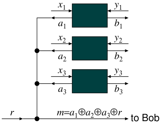
Figure 1: The case of $n\!=\!3$ is shown. The parity bit of all the outputs of the $n$ boxes is scrambled by a random bit $r$ and is sent to Bob as a message.

In the protocol of Fig. 1, since Alice is given $\vec{x}$ and $r$, the relation corresponding to Eq. (20) is

$$I(\vec{x}r:m\rho_{B})=H(m)-H(m|\vec{x}r\rho_{B})=1-H(a_{p}|\vec{x}\rho_{B}),$$ (21)

where we took into account $I(m\!:\!\rho_{B})\!=\!0$ and used $H(m|\vec{x}r\rho_{B})\!=\!H(a_{p}|\vec{x}\rho_{B})$ because the conditional entropy $H(X|Y)\!\equiv\!H(XY)\!-\!H(Y)$ means the remaining uncertainty of $X$ after knowing $Y$ (in the classical variable case). Let us then evaluate $1-H(a_{p}|\vec{x}\rho_{B})$ in quantum mechanics. Considering the individual measurement strategy for boxes, the optimal success probability of guessing Alice’s outcome $a$ of a single box for the input $x$ is given by $(1\!+\!\bar{D}_{x})/2$, which is an operational meaning of the generalized trace distance. As shown in Appendix D, the result of the evaluation in the $n\!\rightarrow\!\infty$ limit is then

$$1-H(a_{p}|\vec{x}\rho_{B})=\frac{1}{2\ln 2}\big{(}\frac{\bar{D}^{2}_{0}+\bar{D}^{2}_{1}}{2}\big{)}^{n},$$ (22)

which appears to well correspond to the right-hand side of Eq. (18) (although there is a slight difference between $\tilde{D}_{x}$ and $\bar{D}_{x}$ in the case of mixed states).

In this way, it is found that the inequalities discussed in this paper represent the effects of the nonzero $H(\vec{m}|\vec{x}\rho_{B})$ in Eq. (20). For the nonzeroness, it is crucial whether or not Bob can completely determine Alice’s outcome (abstractly denoted by $\vec{a}$ hereafter) from the type of her measurement $\vec{x}$ and his local state $\rho_{B}$. If he cannot do this, it implies $H(\vec{a}|\vec{x}\rho_{B})\!>\!0$ and results in $H(\vec{m}|\vec{x}\rho_{B})\!>\!0$ when $\vec{m}$ is constructed from $\vec{a}$ and $\vec{x}$. In this situation, $\vec{a}$ appears to have some randomness and be scrambling the information of $\vec{x}$ encoded in $\vec{m}$ from the viewpoint of Bob. This can occur not only when quantum resources are mixed states, but also pure states. Indeed, quantum correlations, which can be realized by partially entangled states (whose Schmidt coefficients are nondegenerate so that the Schmidt basis is unique), inevitably show $H(\vec{a}|\vec{x}\rho_{B})\!>\!0$, because Alice’s measurements are non-commuting Fine (1982) and the basis of at least one measurement differs from the Schmidt basis. As a result, Bob’s local states for different values of $\vec{a}$ become nonorthogonal, and he cannot completely determine $\vec{a}$. It is a peculiar feature of quantum mechanics that there exist the extremal correlations that are realized by partially entangled states Liang et al. (2011); Acín et al. (2012); Ramanathan et al. ; Zhen et al. (2016) and show $H(\vec{a}|\vec{x}\rho_{B})\!>\!0$, because every extremal correlation of both sets of classical and general no-signaling correlations (local deterministic correlations Brunner et al. (2014) and the Popescu-Rohrlich type boxes Popescu and Rohrlich (1994); Barrett et al. (2005)) does not show $H(\vec{a}|\vec{x}\rho_{B})\!>\!0$.

The randomness discussed above inevitably reduces the information obtainable by Bob. Indeed, it is clear from Eq. (20) that, for a quantum correlation that shows nonzero $H(\vec{a}|\vec{x}\rho_{B})$, any protocol whose $\vec{m}$ contains the information of $\vec{a}$ and $H(\vec{m}|\vec{x}\rho_{B})\!>\!0$ cannot achieve $I(\vec{x}\!:\!\vec{m}\rho_{B})\!=\!H(\vec{m})$ (the achievement is possible when $\vec{m}$ does not contain the information of $\vec{a}$, but in that case the quantum correlation is not used by the protocol). This include the case of the extremal correlations realized by partially entangled states discussed above. For those nonlocal correlations, the strength is constrained by a principle other than the IC principle. To investigate what the principle is, let us consider the protocol of Fig. 1 again. The point is that the message $m$ is completely scrambled by $r$. As a result, $I(\vec{x}:m\rho_{B})=0$ must hold by the cryptographic principle (or the principle of the information theoretic security), which states that a completely scrambled message (i.e., scrambled by independent random bits with the same number of the message bits) cannot carry information Shannon (1949). This cryptographic principle is derived in the same way as in Pawłowski et al. (2009) using the chain rule of mutual information [$I(A\!:\!B|C)=I(A\!:\!BC)-I(A\!:\!C)$] and the exchange symmetry [$I(A\!:\!B|C)=I(B\!:\!A|C)$] as

$$I(\vec{x}:m\rho_{B}) = I(\vec{x}:\rho_{B}|m)+I(\vec{x}:m)$$ (23)

$$= I(\rho_{B}:\vec{x}m)-I(\rho_{B}:m)=0,$$ (24)

where we used $I(\vec{x}m:\rho_{B})=0$ by the no-signaling condition and used $I(m\!:\!\vec{x})\!=\!I(m\!:\!\rho_{B})\!=\!0$ by the independence of $r$. From this cryptographic principle, Eq. (21) is also obtained as

$$0 = I(\vec{x}:m\rho_{B})=I(m\rho_{B}:\vec{x}r)-I(m\rho_{B}:r|\vec{x})$$ (25)

$$= I(\vec{x}r:m\rho_{B})-I(r:\vec{x}m\rho_{B})$$ (26)

$$= I(\vec{x}r:m\rho_{B})-I(m:\vec{x}r\rho_{B})$$ (27)

$$= I(\vec{x}r:m\rho_{B})-1+H(a_{p}|\vec{x}\rho_{B}),$$ (28)

where the independence of $r$ was again used. From this, it is found that $I(\vec{x}r\!:\!m\rho_{B})\!>\!1-H(a_{p}|\vec{x}\rho_{B})$ implies $I(\vec{x}\!:\!m\rho_{B})\!>\!0$; the transmission of information of $\vec{x}r$ beyond $1-H(a_{p}|\vec{x}\rho_{B})$ implies that the completely scrambled message $m$ would carry information of $\vec{x}$. Namely, the strength of the nonlocal correlation is constrained so that the violation of the cryptographic principle does not occur. The inequalities derived in this paper represent the effects of nonzero $H(a_{p}|\vec{x}\rho_{B})$, and those can be said to be cryptographic quantum bounds on nonlocality.

V Boundary condition

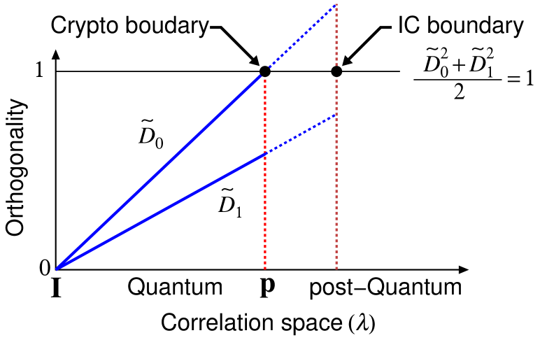
Figure 2: The variation of $\tilde{D}_{0}$ and $\tilde{D}_{1}$ as a function of $\lambda$ in the correlation space of $\lambda\mathbf{p}+(1-\lambda)\mathbf{I}$, where $\mathbf{p}$ is a boundary correlation.

The information theoretical relation representing the cryptographic principle is an equality such as Eq. (28), which is consistent with the fact that the equality of Eq. (8) widely holds not only for boundary correlations but also for non-boundary correlations. However, this is an undesirable property for the purpose of identifying the quantum boundaries. Nevertheless, the cryptographic bounds tell us a way to determine the boundaries. The two-qubit realization shown in Acín et al. (2012) and discussed in Sec. III again gives an informative example. Consider the boundary correlation that maximally violates the Bell expression $\frac{2}{\sqrt{3}}\langle A_{0}\rangle+\langle A_{0}B_{0}\rangle+\langle A_{0}B_{1}\rangle+\langle A_{1}B_{0}\rangle-\langle A_{1}B_{1}\rangle$, where $|\psi\rangle\!=\!\sqrt{2/3}|00\rangle\!+\!\sqrt{1/3}|11\rangle$, $\langle A_{0}\rangle\!=\!1/3$, $\langle A_{1}\rangle\!=\!0$, $\langle B_{0}\rangle\!=\!\langle B_{1}\rangle\!=\!1/\sqrt{17}$, $\langle A_{0}B_{0}\rangle\!=\!\langle A_{0}B_{1}\rangle\!=\!3/\sqrt{17}$, $\langle A_{1}B_{0}\rangle\!=\!-\langle A_{1}B_{1}\rangle\!=\!8/\sqrt{17}/3$, $\tilde{D}_{0}\!=\!1$, and $\tilde{D}_{1}\!=\!\sqrt{8}/3$. This is the same as the simple example shown in Sec. I. For this boundary correlation, the IC inequality is not saturated as $E^{2}_{0}\!+\!E^{2}_{1}\!=\!17/18\!<\!1$, while the cryptographic bound of the IC-type Eq. (5) is saturated as $(\tilde{D}^{2}_{0}\!+\!\tilde{D}^{2}_{1})/2\!=\!17/18$. Note that, since the left-hand side is the same for both inequalities, the saturation of the IC-type inequality implies that the protocol used for the derivation of the IC inequality in Pawłowski et al. (2009) is already optimal for maximizing the left-hand side.

Let us then consider the correlation of the form Eq. (9) with ${\mathbf{p}}$ being the boundary correlation. As discussed in Sec. III, $\tilde{D}_{0}$ and $\tilde{D}_{1}$ of ${\mathbf{q}}$ that saturate Eq. (8) vary linearly with $\lambda$ as schematically shown in Fig. 2. It is then found that the quantum boundary is determined such that $\tilde{D}_{0}$ reaches the maximum limit of 1. Indeed, if $\tilde{D}_{0}$ only takes 1 over all possible realizations of a correlation, the correlation must be located at a boundary, because, if ${\mathbf{q}}$ with $\lambda\!=\!\lambda_{0}\!>\!1$ is quantum realizable, ${\mathbf{p}}$ has a realization with $\tilde{D}_{0}\!=\!1/\lambda_{0}\!<\!1$, which causes a contradiction. This is indeed the case of ${\mathbf{p}}$ because the realization was shown to be unique up to local unitary transformations Acín et al. (2012).

In this way, $\tilde{D}_{0}$ and $\tilde{D}_{1}$, which must not exceed 1, individually set a limit to determine the quantum boundaries. Every boundary in the case of unbiased marginals can be identified in such a way by Lemma 1. This is the case of local deterministic correlations also, where either $\hbox{tr}\rho_{0|x}\!=\!0$ or $\hbox{tr}\rho_{1|x}\!=\!0$ holds and there is no realization with $\tilde{D}_{x}\!<\!1$. Unfortunately, however, the results of the Monte Carlo calculations indicate that both $\tilde{D}_{0}$ and $\tilde{D}_{1}$ (and Alice’s counterparts) are generally less than 1 for extremal correlations with biased marginals, i.e., most are determined by another limit, in spite that the equality of Eq. (8) is respected. What is the principle to fully identify the boundaries? This still remains open.

VI Summary

To conclude, we obtained the nonlocality inequalities in the simplest Bell scenario, which must be respected by quantum mechanics and include the effects of the randomness produced in the message when quantum resources such as partially entangled states and mixed states are used for communication. The randomness originates from the nonorthogonality of receiver’s states and the effects enter the inequalities through the trace distancelike quantity, which is hence close to the bias of the optimal success probability of guessing the sender’s measurement outcome, when assuming that a receiver knows the type of the measurement. The obtained inequalities reflect the constraint by the cryptographic principle. This is due to the fact that the randomness reduces the information obtainable by a receiver, and the transmission of information beyond the reduction implies that a completely scrambled message would carry information.

Introducing the cryptographic principle to nonlocality inequalities leads to two effects. First, the inequalities come to be saturated inside the set of quantum correlations. Indeed, the obtained Landau-type inequality is saturated for all (boundary and non-boundary) correlations with unbiased marginals. We conjecture that the inequality is saturated for every extremal correlation even with biased marginals, i.e., most of nonlocal correlations in the simplest Bell scenario obey a simple and unified rule. Second, the maximum limit of one message bit set by the information causality principle splits into the two trace distancelike quantities, which must not exceed 1 and individually set a limit to determine the quantum boundaries. Namely, the maximalness of the orthogonality (or vanishment of the above mentioned randomness) play an important role in determining some of the quantum boundaries.

Appendix A Properties of $\tilde{D}$

Some properties of the trace distancelike quantity

$$\tilde{D}(\rho,\sigma)=\max_{X}\frac{\hbox{tr}X(\rho-\sigma)}{\sqrt{\hbox{tr}X^{2}(\rho+\sigma)}},$$ (29)

between subnormalized $\rho$ and $\sigma$ are proved here. Without loss of generality, we can assume $\hbox{tr}(\rho+\sigma)\!=\!1$, otherwise renormalize $\rho$ and $\sigma$. Since the maximization is taken over all Hermitian operators $X$, the constraint of $\hbox{tr}X^{2}(\rho+\sigma)\!=\!1$ does not alter the optimization result, and hence let us maximize

$$\hbox{tr}X(\rho-\sigma)-l(\hbox{tr}X^{2}(\rho+\sigma)-1),$$ (30)

where $l$ is the Lagrange multiplier. The extremal condition with respect to the small deviation of $X\!\rightarrow\!X+\Delta X$, where $\Delta X$ is any Hermitian operator, is given by

$$Y\equiv\rho-\sigma-l(\rho+\sigma)X-lX(\rho+\sigma)=0.$$ (31)

In the case of pure states, let $\rho\!=\!p|0\rangle\langle 0|$ and $\sigma\!=\!(1-p)|\phi\rangle\langle\phi|$ where $|\phi\rangle=\cos\phi|0\rangle+\sin\phi|1\rangle$, and let $X=\left(\begin{array}[]{cc}a&b\cr b&c\end{array}\right)$. From $\langle 1|Y|1\rangle\!=\!0$ and $\langle\phi_{\perp}|Y|\phi_{\perp}\rangle\!=\!0$, where $|\phi_{\perp}\rangle=\sin\phi|0\rangle-\cos\phi|1\rangle$, we have $a+c=0$ and hence $X^{2}\!=\!(a^{2}+b^{2})I=I$ so that $\hbox{tr}X^{2}(\rho+\sigma)\!=\!1$. Since

$$\bar{D}(\rho,\sigma)\equiv\hbox{tr}|\rho-\sigma|=\max_{X^{2}=I}\hbox{tr}X(\rho-\sigma),$$ (32)

we have $\tilde{D}(\rho,\sigma)\!=\!\bar{D}(\rho,\sigma)$ in the case of pure states. In the other general cases, $\tilde{D}(\rho,\sigma)\!\geq\!\bar{D}(\rho,\sigma)$ is obvious.

Moreover, let $\rho\!-\!\sigma\!=\!Q\!-\!S$ where $Q$ and $S$ are positive operators with orthogonal support. Since $|\rho\!-\!\sigma|\!\leq\!\rho\!+\!\sigma$, $\hbox{tr}(Q\!+\!S)\!=\!\hbox{tr}|\rho\!-\!\sigma|$, and $\tilde{D}(\rho,\sigma)\!=\!1$ if $\rho$ and $\sigma$ are orthogonal, we have

$$\tilde{D}(\rho,\sigma) \leq \max_{X}\frac{\hbox{tr}X(\rho-\sigma)}{\sqrt{\hbox{tr}X^{2}|\rho-\sigma|}}=\max_{X}\frac{\hbox{tr}X(Q-S)}{\sqrt{\hbox{tr}X^{2}(Q+S)}}$$ (33)

$$= \sqrt{\hbox{tr}(Q+S)}=\sqrt{\bar{D}(\rho,\sigma)}.$$ (34)

Therefore, $\bar{D}(\rho,\sigma)\!\leq\!\tilde{D}(\rho,\sigma)\!\leq\!\sqrt{\bar{D}(\rho,\sigma)}$, and hence $\tilde{D}(\rho,\sigma)\!=\!1$ if and only if $\bar{D}(\rho,\sigma)\!=\!1$.

The optimization with respect to $X$ in Eq. (29) can be performed analytically as follows. Let $|i\rangle$ be the eigenstate of $\rho+\sigma$, i.e., $(\rho+\sigma)|i\rangle=\lambda_{i}|i\rangle$, and $x_{ij}\equiv\langle i|X|j\rangle$. We then have

$$\hbox{tr}X^{2}(\rho+\sigma) = \sum_{i}\lambda_{i}(x_{ii})^{2}+\sum_{j>i}(\lambda_{i}+\lambda_{j})|x_{ij}|^{2}$$ (35)

$$= \sum_{i}(x^{\prime}_{ii})^{2}+\sum_{j>i}|x^{\prime}_{ij}|^{2}=1,$$ (36)

where $x^{\prime}_{ii}\equiv\sqrt{\lambda_{i}}x_{ii}$ and $x^{\prime}_{ij}\equiv\sqrt{\lambda_{i}\!+\!\lambda_{j}}x_{ij}$ for $i\!\neq\!j$. Moreover, using $a_{ij}=\langle i|\rho-\sigma|j\rangle$, we have

$$\hbox{tr}X(\rho-\sigma) = \sum_{i}x_{ii}a_{ii}+\sum_{j>i}(x_{ij}a^{*}_{ij}+x^{*}_{ij}a_{ij})$$ (37)

$$= \sum_{i}\frac{x^{\prime}_{ii}a_{ii}}{\sqrt{\lambda_{i}}}+\sum_{j>i}\frac{x^{\prime}_{ij}a^{*}_{ij}+x^{\prime*}_{ij}a_{ij}}{\sqrt{\lambda_{i}+\lambda_{j}}}.$$ (38)

Since $\tilde{D}(\rho,\sigma)$ is given by the maximum of Eq. (38) under the constraint of Eq. (36), we have

$$\tilde{D}(\rho,\sigma)=\big{(}\sum_{i}\frac{(a_{ii})^{2}}{\lambda_{i}}+\sum_{j>i}\frac{4|a_{ij}|^{2}}{\lambda_{i}+\lambda_{j}}\big{)}^{\frac{1}{2}}=\big{(}\sum_{ij}\frac{2|a_{ij}|^{2}}{\lambda_{i}+\lambda_{j}}\big{)}^{\frac{1}{2}}.$$

Appendix B Landau-type inequality

In the CHSH expression with general weight parameters, if we define $X_{x}\!=\!u_{x0}B_{0}\!+\!(-1)^{x}u_{x1}B_{1}$, we have $X^{2}_{0}\!+\!X^{2}_{1}\!=\!\sum_{xy}u^{2}_{xy}I$ by virtue of $u_{00}u_{01}\!=\!u_{10}u_{11}$, and hence obtain Eq. (6). When $\tilde{D}_{0},\tilde{D}_{1}\!>\!0$, we have

$$\sum_{x}\big{(}u_{x0}\tilde{C}_{x0}+(-1)^{x}u_{x1}\tilde{C}_{x1}\big{)}^{2}\leq\sum_{xy}u^{2}_{xy}.$$ (39)

Noticing $\tilde{C}^{2}_{xy}\!\leq\!1$ and using $v_{xy}\!\equiv\!u_{xy}(1\!-\!\tilde{C}^{2}_{xy})^{\frac{1}{2}}$, this is rewritten as

$$(\tilde{C}_{00}\tilde{C}_{01}\!-\!\tilde{C}_{10}\tilde{C}_{11})v_{00}v_{01}\leq(1\!-\!\tilde{C}^{2}_{00})^{\frac{1}{2}}(1\!-\!\tilde{C}^{2}_{01})^{\frac{1}{2}}\sum_{xy}{\textstyle\frac{1}{2}}v^{2}_{xy}.$$

Since $u_{00}u_{01}\!=\!u_{10}u_{11}$, it can be seen that

$$(1\!-\!\tilde{C}^{2}_{00})^{\frac{1}{2}}(1\!-\!\tilde{C}^{2}_{01})^{\frac{1}{2}}\sum_{xy}{\textstyle\frac{1}{2}}v^{2}_{xy}$$

$$\!\!\geq\!\! (1\!-\!\tilde{C}^{2}_{00})^{\frac{1}{2}}(1\!-\!\tilde{C}^{2}_{01})^{\frac{1}{2}}(|v_{00}v_{01}|+|v_{10}v_{11}|)$$

$$\!\!=\!\! [(1\!-\!\tilde{C}^{2}_{00})^{\frac{1}{2}}(1\!-\!\tilde{C}^{2}_{01})^{\frac{1}{2}}+(1\!-\!\tilde{C}^{2}_{10})^{\frac{1}{2}}(1\!-\!\tilde{C}^{2}_{11})^{\frac{1}{2}}]|v_{00}v_{01}|,$$

and we obtain Eq. (8). In the case of $\tilde{D}_{x_{0}}\!=\!0$ for either $x_{0}\!=\!0$ or $1$, $C_{x_{0}y}\!=\!0$ holds because $\tilde{D}_{x_{0}}\!\geq\!|C_{x_{0}y}|$ by definition, and we have Eq. (8) in which $\tilde{C}_{x_{0}0}\!=\!\tilde{C}_{x_{0}1}\!=\!0$.

Similarly, for a tilted CHSH expression, we have

$$\sum_{xy}s_{x}u_{xy}(-1)^{xy}\langle(A_{x}\!+\!\epsilon_{x}I)\otimes B_{y}\rangle$$ (40)

$$\leq \big{[}\sum_{xy}u^{2}_{xy}\big{]}^{\frac{1}{2}}\big{[}\sum_{x}s^{2}_{x}(\tilde{D}^{\epsilon}_{x})^{2})\big{]}^{\frac{1}{2}},$$ (41)

where $u_{00}u_{01}\!=\!u_{10}u_{11}$ again, $\epsilon_{x}$ is real, and

$$\tilde{D}^{\epsilon}_{x}\!\equiv\!\max_{X}\frac{\hbox{tr}X[(1+\epsilon_{x})\rho_{0|x}-(1-\epsilon_{x})\rho_{1|x}]}{\sqrt{\hbox{tr}X^{2}(\rho_{0|x}+\rho_{1|x})}}.$$ (42)

In the same way as Appendix A, it is not difficult to see $(\tilde{D}^{\epsilon}_{x})^{2}\!=\!\tilde{D}_{x}^{2}\!+\!2\epsilon_{x}\langle A_{x}\rangle\!+\!\epsilon_{x}^{2}$. When $\tilde{D}^{2}_{0}\!>\!\langle A_{0}\rangle^{2}$ and $\tilde{D}^{2}_{1}\!>\!\langle A_{1}\rangle^{2}$, the necessary and sufficient condition of Eq. (41) is again Eq. (8) but with

$$\tilde{C}_{xy}\equiv\frac{C_{xy}-\langle A_{x}\rangle\langle B_{y}\rangle}{(\tilde{D}^{2}_{x}-\langle A_{x}\rangle^{2})^{\frac{1}{2}}(1-\langle B_{y}\rangle^{2})^{\frac{1}{2}}}.$$ (43)

This is an extension of the NPA inequality Navascués et al. (2007, 2008).

Appendix C Extremal correlation

Under the parametrization of Eq. (11), the expectation of the Bell expression $\sum_{abxy}V_{abxy}p(ab|xy)$ with $p(ab|xy)\!=\!\langle\psi|P_{a|x}\!\otimes\!Q_{b|y}|\psi\rangle$ is maximized when $\rho\!=\!|\psi\rangle\langle\psi|$ is real symmetric. A necessary and sufficient condition for the saturation of Eq. (8) is that it is possible to assign nontrivial values to $u_{xy}$ such that Eq. (6) is saturated (and $u_{00}u_{01}\!=\!u_{10}u_{11}$). This is possible only when $X_{x}\!=\!\sum_{y}(-1)^{xy}u_{xy}B_{y}$ agrees with the operator of maximizing $\tilde{D}_{x}$. Note that $\rho$ is pure and the projector is rank 1, $\rho_{a|x}$ is also pure and $\tilde{D}_{x}\!=\!\bar{D}_{x}$. Since the operator of maximizing $\tilde{D}_{x}$ is then unique up to the normalization, we have $X_{x}\!\propto\!\cos\phi^{B}_{x}\sigma_{1}\!+\!\sin\phi^{B}_{x}\sigma_{3}$ hence $\sum_{y}(-1)^{xy}u_{xy}\sin(\phi^{B}_{x}\!-\!\theta^{B}_{y})\!=\!0$. In order that $u_{00}u_{01}\!=\!u_{10}u_{11}$, $-\sin(\phi^{B}_{1}\!-\!\theta^{B}_{0})\sin(\phi^{B}_{0}\!-\!\theta^{B}_{0})u^{2}_{00}\!=\!\sin(\phi^{B}_{0}\!-\!\theta^{B}_{1})\sin(\phi^{B}_{1}\!-\!\theta^{B}_{1})u^{2}_{11}$ and $-\sin(\phi^{B}_{0}\!-\!\theta^{B}_{1})\sin(\phi^{B}_{1}\!-\!\theta^{B}_{1})u^{2}_{01}\!=\!\sin(\phi^{B}_{1}\!-\!\theta^{B}_{0})\sin(\phi^{B}_{0}\!-\!\theta^{B}_{0})u^{2}_{10}$ must hold, and we obtain Eq. (14). Since there are no other constraints for $u_{xy}$, we can assign nontrivial values to $u_{xy}$ if Eq. (14) is satisfied.

Appendix D Evaluation of $1-H(a_{p}|\vec{x}\rho_{B})$

Let us denote Bob’s guess for the parity bit $a_{p}$ (for a given $\vec{x}$) under the individual measurement strategy for boxes by $b_{p}$, the conditional probability by $P_{a_{p}|b_{p}}$, and the other probabilities similarly. Let us then evaluate the leading term of $H(a_{p}|b_{p})$ given by

$$H(a_{p}|b_{p})=P_{b_{p}=0}h(P_{0|0})+P_{b_{p}=1}h(P_{1|1})$$

$$\!\!\!\approx\!\!\! 1-\frac{1}{2\ln 2}\big{[}P_{b_{p}=0}(2P_{0|0}-1)^{2}+P_{b_{p}=1}(2P_{1|1}-1)^{2}\big{]}$$

$$\!\!\!=\!\!\! 1-\frac{1}{2\ln 2}\big{[}\frac{(P_{a_{p}=b_{p}}-P_{a_{p}=1})^{2}}{P_{b_{p}=0}}+\frac{(P_{a_{p}=b_{p}}-P_{a_{p}=0})^{2}}{P_{b_{p}=1}}\big{]},$$

for $k\!\gg\!1$ and $n\!-\!k\!\gg\!1$ with $k$ being the number of 0 in a given $\vec{x}$ (see also Bennett et al. (1996)). Since the optimal success probability of guessing $a$ for a single box is $(1\!+\!\bar{D}_{x})/2$, the optimal probability for $a_{p}$ is given by $P_{a_{p}=b_{p}}\!=\!(1+\bar{D}^{k}_{0}\bar{D}^{n-k}_{1})/2$. Using Alice’s marginals $p(a|x)$ of a single box, we have

$$P_{a_{p}=0}=\frac{1}{2}\big{[}1+\left(2p(0|0)-1\right)^{k}\left(2p(0|1)-1\right)^{n-k}\big{]}.$$ (44)

Suppose that $\rho_{0|x}$ and $\rho_{1|x}$ are nonorthogonal. Moreover, $\hbox{sup}(\rho_{0|x})$ and $\hbox{sup}(\rho_{1|x})$ are not identical in general. This implies $|2p(0|x)\!-\!1|\!<\!\bar{D}_{x}\!<\!1$, and hence the leading term comes from $\bar{D}^{k}_{0}\bar{D}^{n-k}_{1}$. As a result, since $H(a_{p}|b_{p})\approx 1-\bar{D}^{2k}_{0}\bar{D}^{2(n-k)}_{1}/(2\ln 2)$, we have

$$1-H(a_{p}|\vec{x}\rho_{B})=1-\frac{1}{2^{n}}\sum_{\vec{x}}H(a_{p}|b_{p})$$

$$\!\!\!\approx\!\!\! \frac{1}{2\ln 2}\frac{1}{2^{n}}\sum_{k=0}^{n}\binom{n}{k}\bar{D}^{2k}_{0}\bar{D}^{2(n-k)}_{1}=\frac{1}{2\ln 2}\big{(}\frac{\bar{D}^{2}_{0}+\bar{D}^{2}_{1}}{2}\big{)}^{n}.$$

References

• Bell (1964) J. Bell, Physics 1, 195 (1964).
• Cirel’son (1980) B. S. Cirel’son, Lett. Math. Phys. 4, 93 (1980).
• Popescu and Rohrlich (1994) S. Popescu and D. Rohrlich, Found. Phys. 24, 379 (1994).
• Clauser et al. (1969) J. F. Clauser, M. A. Horne, A. Shimony, and R. A. Holt, Phys. Rev. Lett. 23, 880 (1969).
• Brunner et al. (2014) N. Brunner, D. Cavalcanti, S. Pironio, V. Scarani, and S. Wehner, Rev. Mod. Phys. 86, 419 (2014).
• Popescu (2014) S. Popescu, Nat. Phys. 10, 264 (2014).
• Oas and de Barros (2016) G. Oas and J. A. de Barros, Contextuality from Quantum Physics to Psychology (World Scientific, Singapore, 2016), chap. 15, pp. 335–366.
• Pawłowski et al. (2009) M. Pawłowski, T. Paterek, D. Kaszlikowski, V. Scarani, A. Winter, and M. Zukowski, Nature (London) 461, 1101 (2009).
• Allcock et al. (2009) J. Allcock, N. Brunner, M. Pawlowski, and V. Scarani, Phys. Rev. A 80, 040103 (2009).
• Tsirelson (1987) B. S. Tsirelson, J. Sov. Math. 36, 557 (1987).
• Landau (1988) L. J. Landau, Found. Phys. 18, 449 (1988).
• (12) L. Masanes, arXiv:quant-ph/0309137.
• Liang et al. (2011) Y.-C. Liang, T. Vértesi, and N. Brunner, Phys. Rev. A 83, 022108 (2011).
• Acín et al. (2012) A. Acín, S. Massar, and S. Pironio, Phys. Rev. Lett. 108, 100402 (2012).
• (15) R. Ramanathan, D. Goyeneche, P. Mironowicz, and P. Horodecki, arXiv:1506.05100.
• Zhen et al. (2016) Y.-Z. Zhen, K. T. Goh, Y.-L. Zheng, W.-F. Cao, X. Wu, K. Chen, and V. Scarani, Phys. Rev. A 94, 022116 (2016).
• Gallego et al. (2011) R. Gallego, L. E. Würflinger, A. Acín, and M. Navascués, Phys. Rev. Lett. 107, 210403 (2011).
• Yang et al. (2012) T. H. Yang, D. Cavalcanti, M. L. Almeida, C. Teo, and V. Scarani, New J. Phys. 14, 013061 (2012).
• Shannon (1949) C. E. Shannon, Bell System Technical Journal 28, 656 (1949).
• (20) A. Y. Carmi and D. Moskovich, arXiv:1507.07514.
• Lowson et al. (2010) T. Lowson, N. Linden, and S. Popescu, arXiv:1011.6245 (2010).
• Vértesi and Pál (2008) T. Vértesi and K. F. Pál, Phys. Rev. A 77, 042106 (2008).
• Liang and Doherty (2007) Y.-C. Liang and A. C. Doherty, Phys. Rev. A 75, 042103 (2007).
• Navascués et al. (2007) M. Navascués, S. Pironio, and A. Acín, Phys. Rev. Lett. 98, 010401 (2007).
• Navascués et al. (2008) M. Navascués, S. Pironio, and A. Acín, New J. Phys. 10, 073013 (2008).
• Wang et al. (2016) Y. Wang, X. Wu, and V. Scarani, New J. Phys. 18, 025021 (2016).
• Masanes (2006) L. Masanes, Phys. Rev. Lett. 97, 050503 (2006).
• Buhrman et al. (2010) H. Buhrman, R. Cleve, S. Massar, and R. de Wolf, Rev. Mod. Phys. 82, 665 (2010).
• van Dam (2013) W. van Dam, Natural Computing 12, 9 (2013).
• Dahlsten et al. (2012) O. C. O. Dahlsten, D. Lercher, and R. Renner, New J. Phys. 14, 063024 (2012).
• Al-Safi and Short (2011) S. W. Al-Safi and A. J. Short, Phys. Rev. A 84, 042323 (2011).
• Pawłowski and Winter (2012) M. Pawłowski and A. Winter, Phys. Rev. A 85, 022331 (2012).
• Bavarian and Shor (2015) M. Bavarian and P. W. Shor, Proc. of 2015 Conference on Innovations in Theoretical Computer Science (ITCS ’15) p. 123 (2015).
• Chavesl et al. (2014) R. Chavesl, C. Majenz, and D. Gross, Nat. Commun. 6, 5766 (2014).
• Fine (1982) A. Fine, Phys. Rev. Lett. 48, 291 (1982).
• Barrett et al. (2005) J. Barrett, N. Linden, S. Massar, S. Pironio, S. Popescu, and D. Roberts, Phys. Rev. A 71, 022101 (2005).
• Bennett et al. (1996) C. H. Bennett, T. Mor, and J. A. Smolin, Phys. Rev. A 54, 2675 (1996).