Flavour Physics and CP Violation

Abstract

We explain the many reasons for the interest in flavor physics. We describe flavor physics and the related CP violation within the Standard Model, and explain how the B-factories proved that the Kobayashi-Maskawa mechanism dominates the CP violation that is observed in meson decays. We explain the implications of flavor physics for new physics, with emphasis on the “new physics flavor puzzle”, and present the idea of minimal flavor violation as a possible solution. We explain why the values flavor parameters of the Standard Model are puzzling, present the Froggatt-Nielsen mechanism as a possible solution, and describe how measurements of neutrino parameters are interpreted in the context of this puzzle. We show that the recently discovered Higgs-like boson may provide new opportunities for making progress on the various flavor puzzles.

0.1 What is flavor?

The term “flavors” is used, in the jargon of particle physics, to describe several copies of the same gauge representation, namely several fields that are assigned the same quantum charges. Within the Standard Model, when thinking of its unbroken $SU(3)_{\rm C}\times U(1)_{\rm EM}$ gauge group, there are four different types of particles, each coming in three flavors:

• Up-type quarks in the $(3)_{+2/3}$ representation: $u,c,t$;

• Down-type quarks in the $(3)_{-1/3}$ representation: $d,s,b$;

• Charged leptons in the $(1)_{-1}$ representation: $e,\mu,\tau$;

• Neutrinos in the $(1)_{0}$ representation: $\nu_{1},\nu_{2},\nu_{3}$.

The term “flavor physics” refers to interactions that distinguish between flavors. By definition, gauge interactions, namely interactions that are related to unbroken symmetries and mediated therefore by massless gauge bosons, do not distinguish among the flavors and do not constitute part of flavor physics. Within the Standard Model, flavor-physics refers to the weak and Yukawa interactions.

The term “flavor parameters” refers to parameters that carry flavor indices. Within the Standard Model, these are the nine masses of the charged fermions and the four “mixing parameters” (three angles and one phase) that describe the interactions of the charged weak-force carriers ($W^{\pm}$) with quark-antiquark pairs. If one augments the Standard Model with Majorana mass terms for the neutrinos, one should add to the list three neutrino masses and six mixing parameters (three angles and three phases) for the $W^{\pm}$ interactions with lepton-antilepton pairs.

The term “flavor universal” refers to interactions with couplings (or to parameters) that are proportional to the unit matrix in flavor space. Thus, the strong and electromagnetic interactions are flavor-universal. An alternative term for “flavor-universal” is “flavor-blind”.

The term “flavor diagonal” refers to interactions with couplings (or to parameters) that are diagonal, but not necessarily universal, in the flavor space. Within the Standard Model, the Yukawa interactions of the Higgs particle are flavor diagonal.

The term “flavor changing” refers to processes where the initial and final flavor-numbers (that is, the number of particles of a certain flavor minus the number of anti-particles of the same flavor) are different. In “flavor changing charged current” processes, both up-type and down-type flavors, and/or both charged lepton and neutrino flavors are involved. Examples are (i) muon decay via $\mu\to e\bar{\nu}_{i}\nu_{j}$, and (ii) $K^{-}\to\mu^{-}\bar{\nu}_{j}$ (which corresponds, at the quark level, to $s\bar{u}\to\mu^{-}\bar{\nu}_{j}$). Within the Standard Model, these processes are mediated by the $W$-bosons and occur at tree level. In “flavor changing neutral current” (FCNC) processes, either up-type or down-type flavors but not both, and/or either charged lepton or neutrino flavors but not both, are involved. Example are (i) muon decay via $\mu\to e\gamma$ and (ii) $K_{L}\to\mu^{+}\mu^{-}$ (which corresponds, at the quark level, to $s\bar{d}\to\mu^{+}\mu^{-}$). Within the Standard Model, these processes do not occur at tree level, and are often highly suppressed.

Another useful term is “flavor violation”. We explain it later in these lectures.

0.2 Why is flavor physics interesting?

• Flavor physics can discover new physics or probe it before it is directly observed in experiments. Here are some examples from the past:

  • The smallness of $\frac{\Gamma(K_{L}\to\mu^{+}\mu^{-})}{\Gamma(K^{+}\to\mu^{+}\nu)}$ led to predicting a fourth (the charm) quark;

  • The size of $\Delta m_{K}$ led to a successful prediction of the charm mass;

  • The size of $\Delta m_{B}$ led to a successful prediction of the top mass;

  • The measurement of $\varepsilon_{K}$ led to predicting the third generation.

  • The measurement of neutrino flavor transitions led to the discovery of neutrino masses.

• CP violation is closely related to flavor physics. Within the Standard Model, there is a single CP violating parameter, the Kobayashi-Maskawa phase $\delta_{\rm KM}$ [1]. Baryogenesis tells us, however, that there must exist new sources of CP violation. Measurements of CP violation in flavor changing processes might provide evidence for such sources.

• The fine-tuning problem of the Higgs mass, and the puzzle of the dark matter imply that there exists new physics at, or below, the TeV scale. If such new physics had a generic flavor structure, it would contribute to flavor changing neutral current (FCNC) processes orders of magnitude above the observed rates. The question of why this does not happen constitutes the new physics flavor puzzle.

• Most of the charged fermion flavor parameters are small and hierarchical. The Standard Model does not provide any explanation of these features. This is the Standard Model flavor puzzle. The puzzle became even deeper after neutrino masses and mixings were measured because, so far, neither smallness nor hierarchy in these parameters have been established.

0.3 Flavor in the Standard Model

A model of elementary particles and their interactions is defined by the following ingredients: (i) The symmetries of the Lagrangian and the pattern of spontaneous symmetry breaking; (ii) The representations of fermions and scalars. The Standard Model (SM) is defined as follows:
(i) The gauge symmetry is

$$G_{\rm SM}=SU(3)_{\rm C}\times SU(2)_{\rm L}\times U(1)_{\rm Y}.$$ (1)

It is spontaneously broken by the VEV of a single Higgs scalar, $\phi(1,2)_{1/2}$ $\left(\langle\phi^{0}\rangle=v/\sqrt{2}\right)$:

$$G_{\rm SM}\to SU(3)_{\rm C}\times U(1)_{\rm EM}.$$ (2)

(ii) There are three fermion generations, each consisting of five representations of $G_{\rm SM}$:

$$Q_{Li}(3,2)_{+1/6},\ \ U_{Ri}(3,1)_{+2/3},\ \ D_{Ri}(3,1)_{-1/3},\ \ L_{Li}(1,2)_{-1/2},\ \ E_{Ri}(1,1)_{-1}.$$ (3)

0.3.1 The interaction basis

The Standard Model Lagrangian, ${\cal L}_{\rm SM}$, is the most general renormalizable Lagrangian that is consistent with the gauge symmetry (1), the particle content (3) and the pattern of spontaneous symmetry breaking (2). It can be divided to three parts:

$${\cal L}_{\rm SM}={\cal L}_{\rm kinetic}+{\cal L}_{\rm Higgs}+{\cal L}_{\rm Yukawa}.$$ (4)

As concerns the kinetic terms, to maintain gauge invariance, one has to replace the derivative with a covariant derivative:

$$D^{\mu}=\partial^{\mu}+ig_{s}G^{\mu}_{a}L_{a}+igW^{\mu}_{b}T_{b}+ig^{\prime}B^{\mu}Y.$$ (5)

Here $G^{\mu}_{a}$ are the eight gluon fields, $W^{\mu}_{b}$ the three weak interaction bosons and $B^{\mu}$ the single hypercharge boson. The $L_{a}$’s are $SU(3)_{\rm C}$ generators (the $3\times 3$ Gell-Mann matrices ${1\over 2}\lambda_{a}$ for triplets, $0$ for singlets), the $T_{b}$’s are $SU(2)_{\rm L}$ generators (the $2\times 2$ Pauli matrices ${1\over 2}\tau_{b}$ for doublets, $0$ for singlets), and the $Y$’s are the $U(1)_{\rm Y}$ charges. For example, for the quark doublets $Q_{L}$, we have

$${\cal L}_{\rm kinetic}(Q_{L})=i{\overline{Q_{Li}}}\gamma_{\mu}\left(\partial^{\mu}+{i\over 2}g_{s}G^{\mu}_{a}\lambda_{a}+{i\over 2}gW^{\mu}_{b}\tau_{b}+{i\over 6}g^{\prime}B^{\mu}\right)\delta_{ij}Q_{Lj},$$ (6)

while for the lepton doublets $L_{L}^{I}$, we have

$${\cal L}_{\rm kinetic}(L_{L})=i{\overline{L_{Li}}}\gamma_{\mu}\left(\partial^{\mu}+{i\over 2}gW^{\mu}_{b}\tau_{b}-\frac{i}{2}g^{\prime}B^{\mu}\right)\delta_{ij}L_{Lj}.$$ (7)

The unit matrix in flavor space, $\delta_{ij}$, signifies that these parts of the interaction Lagrangian are flavor-universal. In addition, they conserve CP.

The Higgs potential, which describes the scalar self interactions, is given by:

$${\cal L}_{\rm Higgs}=\mu^{2}\phi^{\dagger}\phi-\lambda(\phi^{\dagger}\phi)^{2}.$$ (8)

For the Standard Model scalar sector, where there is a single doublet, this part of the Lagrangian is also CP conserving.

The quark Yukawa interactions are given by

$$-{\cal L}_{\rm Y}^{q}=Y^{d}_{ij}{\overline{Q_{Li}}}\phi D_{Rj}+Y^{u}_{ij}{\overline{Q_{Li}}}\tilde{\phi}U_{Rj}+{\rm h.c.},$$ (9)

(where $\tilde{\phi}=i\tau_{2}\phi^{\dagger}$) while the lepton Yukawa interactions are given by

$$-{\cal L}_{\rm Y}^{\ell}=Y^{e}_{ij}{\overline{L_{Li}}}\phi E_{Rj}+{\rm h.c.}.$$ (10)

This part of the Lagrangian is, in general, flavor-dependent (that is, $Y^{f}\not\propto{\bf 1}$) and CP violating.

0.3.2 Global symmetries

In the absence of the Yukawa matrices $Y^{d}$, $Y^{u}$ and $Y^{e}$, the SM has a large $U(3)^{5}$ global symmetry:

$$G_{\rm global}(Y^{u,d,e}=0)=SU(3)_{q}^{3}\times SU(3)_{\ell}^{2}\times U(1)^{5},$$ (11)

where

$$SU(3)_{q}^{3} = SU(3)_{Q}\times SU(3)_{U}\times SU(3)_{D},$$

$$SU(3)_{\ell}^{2} = SU(3)_{L}\times SU(3)_{E},$$

$$U(1)^{5} = U(1)_{B}\times U(1)_{L}\times U(1)_{Y}\times U(1)_{\rm PQ}\times U(1)_{E}.$$ (12)

Out of the five $U(1)$ charges, three can be identified with baryon number ($B$), lepton number ($L$) and hypercharge ($Y$), which are respected by the Yukawa interactions. The two remaining $U(1)$ groups can be identified with the PQ symmetry whereby the Higgs and $D_{R},E_{R}$ fields have opposite charges, and with a global rotation of $E_{R}$ only.

The point that is important for our purposes is that ${\cal L}_{\rm kinetic}+{\cal L}_{\rm Higgs}$ respect the non-Abelian flavor symmetry $S(3)_{q}^{3}\times SU(3)_{\ell}^{2}$, under which

$$Q_{L}\to V_{Q}Q_{L},\ \ \ U_{R}\to V_{U}U_{R},\ \ \ D_{R}\to V_{D}D_{R},\ \ L_{L}\to V_{L}L_{L},\ \ \ E_{R}\to V_{E}E_{R},$$ (13)

where the $V_{i}$ are unitary matrices. The Yukawa interactions (9) and (10) break the global symmetry,

$$G_{\rm global}(Y^{u,d,e}\neq 0)=U(1)_{B}\times U(1)_{e}\times U(1)_{\mu}\times U(1)_{\tau}.$$ (14)

(Of course, the gauged $U(1)_{Y}$ also remains a good symmetry.) Thus, the transformations of Eq. (13) are not a symmetry of ${\cal L}_{\rm SM}$. Instead, they correspond to a change of the interaction basis. These observations also offer an alternative way of defining flavor physics: it refers to interactions that break the $SU(3)^{5}$ symmetry (13). Thus, the term “flavor violation” is often used to describe processes or parameters that break the symmetry.

One can think of the quark Yukawa couplings as spurions that break the global $SU(3)_{q}^{3}$ symmetry (but are neutral under $U(1)_{B}$),

$$Y^{u}\sim(3,\bar{3},1)_{SU(3)_{q}^{3}},\ \ \ Y^{d}\sim(3,1,\bar{3})_{SU(3)_{q}^{3}},$$ (15)

and of the lepton Yukawa couplings as spurions that break the global $SU(3)_{\ell}^{2}$ symmetry (but are neutral under $U(1)_{e}\times U(1)_{\mu}\times U(1)_{\tau}$),

$$Y^{e}\sim(3,\bar{3})_{SU(3)_{\ell}^{2}}.$$ (16)

The spurion formalism is convenient for several purposes: parameter counting (see below), identification of flavor suppression factors (see Section 0.5), and the idea of minimal flavor violation (see Section 0.5.3).

0.3.3 Counting parameters

How many independent parameters are there in ${\cal L}_{\rm Y}^{q}$? The two Yukawa matrices, $Y^{u}$ and $Y^{d}$, are $3\times 3$ and complex. Consequently, there are 18 real and 18 imaginary parameters in these matrices. Not all of them are, however, physical. The pattern of $G_{\rm global}$ breaking means that there is freedom to remove 9 real and 17 imaginary parameters (the number of parameters in three $3\times 3$ unitary matrices minus the phase related to $U(1)_{B}$). For example, we can use the unitary transformations $Q_{L}\to V_{Q}Q_{L}$, $U_{R}\to V_{U}U_{R}$ and $D_{R}\to V_{D}D_{R}$, to lead to the following interaction basis:

$$Y^{d}=\lambda_{d},\ \ \ Y^{u}=V^{\dagger}\lambda_{u},$$ (17)

where $\lambda_{d,u}$ are diagonal,

$$\lambda_{d}={\rm diag}(y_{d},y_{s},y_{b}),\ \ \ \lambda_{u}={\rm diag}(y_{u},y_{c},y_{t}),$$ (18)

while $V$ is a unitary matrix that depends on three real angles and one complex phase. We conclude that there are 10 quark flavor parameters: 9 real ones and a single phase. In the mass basis, we will identify the nine real parameters as six quark masses and three mixing angles, while the single phase is $\delta_{\rm KM}$.

How many independent parameters are there in ${\cal L}_{\rm Y}^{\ell}$? The Yukawa matrix $Y^{e}$ is $3\times 3$ and complex. Consequently, there are 9 real and 9 imaginary parameters in this matrix. There is, however, freedom to remove 6 real and 9 imaginary parameters (the number of parameters in two $3\times 3$ unitary matrices minus the phases related to $U(1)^{3}$). For example, we can use the unitary transformations $L_{L}\to V_{L}L_{L}$ and $E_{R}\to V_{E}E_{R}$, to lead to the following interaction basis:

$$Y^{e}=\lambda_{e}={\rm diag}(y_{e},y_{\mu},y_{\tau}).$$ (19)

We conclude that there are 3 real lepton flavor parameters. In the mass basis, we will identify these parameters as the three charged lepton masses. We must, however, modify the model when we take into account the evidence for neutrino masses.

0.3.4 The mass basis

Upon the replacement ${\cal R}e(\phi^{0})\to\frac{v+h^{0}}{\sqrt{2}}$, the Yukawa interactions (9) give rise to the mass matrices

$$M_{q}={v\over\sqrt{2}}Y^{q}.$$ (20)

The mass basis corresponds, by definition, to diagonal mass matrices. We can always find unitary matrices $V_{qL}$ and $V_{qR}$ such that

$$V_{qL}M_{q}V_{qR}^{\dagger}=M_{q}^{\rm diag}\equiv\frac{v}{\sqrt{2}}\lambda_{q}.$$ (21)

The four matrices $V_{dL}$, $V_{dR}$, $V_{uL}$ and $V_{uR}$ are then the ones required to transform to the mass basis. For example, if we start from the special basis (17), we have $V_{dL}=V_{dR}=V_{uR}={\bf 1}$ and $V_{uL}=V$. The combination $V_{uL}V_{dL}^{\dagger}$ is independent of the interaction basis from which we start this procedure.

We denote the left-handed quark mass eigenstates as $U_{L}$ and $D_{L}$. The charged current interactions for quarks [that is the interactions of the charged $SU(2)_{\rm L}$ gauge bosons $W^{\pm}_{\mu}={1\over\sqrt{2}}(W^{1}_{\mu}\mp iW_{\mu}^{2})$], which in the interaction basis are described by (6), have a complicated form in the mass basis:

$$-{\cal L}_{W^{\pm}}^{q}={g\over\sqrt{2}}{\overline{U_{Li}}}\gamma^{\mu}V_{ij}D_{Lj}W_{\mu}^{+}+{\rm h.c.}.$$ (22)

where $V$ is the $3\times 3$ unitary matrix ($VV^{\dagger}=V^{\dagger}V={\bf 1}$) that appeared in Eq. (17). For a general interaction basis,

$$V=V_{uL}V_{dL}^{\dagger}.$$ (23)

$V$ is the Cabibbo-Kobayashi-Maskawa (CKM) mixing matrix for quarks [2, 1]. As a result of the fact that $V$ is not diagonal, the $W^{\pm}$ gauge bosons couple to quark mass eigenstates of different generations. Within the Standard Model, this is the only source of flavor changing quark interactions.

Exercise 1: Prove that, in the absence of neutrino masses, there is no mixing in the lepton sector.

Exercise 2: Prove that there is no mixing in the $Z$ couplings. (In the physics jargon, there are no flavor changing neutral currents at tree level.)

The detailed structure of the CKM matrix, its parametrization, and the constraints on its elements are described in Appendix .9.

0.4 Testing CKM

Measurements of rates, mixing, and CP asymmetries in $B$ decays in the two B factories, BaBar abd Belle, and in the two Tevatron detectors, CDF and D0, signified a new era in our understanding of CP violation. The progress is both qualitative and quantitative. Various basic questions concerning CP and flavor violation have received, for the first time, answers based on experimental information. These questions include, for example,

• Is the Kobayashi-Maskawa mechanism at work (namely, is $\delta_{\rm KM}\neq 0$)?

• Does the KM phase dominate the observed CP violation?

As a first step, one may assume the SM and test the overall consistency of the various measurements. However, the richness of data from the B factories allow us to go a step further and answer these questions model independently, namely allowing new physics to contribute to the relevant processes. We here explain the way in which this analysis proceeds.

0.4.1 $S_{\psi K_{S}}$

The CP asymmetry in $B\to\psi K_{S}$ decays plays a major role in testing the KM mechanism. Before we explain the test itself, we should understand why the theoretical interpretation of the asymmetry is exceptionally clean, and what are the theoretical parameters on which it depends, within and beyond the Standard Model.

The CP asymmetry in neutral meson decays into final CP eigenstates $f_{CP\ }$ is defined as follows:

$${\cal A}_{f_{CP\ }}(t)\equiv\frac{d\Gamma/dt[\overline{B}{}^{0}_{\rm phys}(t)\to f_{CP\ }]-d\Gamma/dt[{B^{0}}_{\rm phys}(t)\to f_{CP\ }]}{d\Gamma/dt[\overline{B}{}^{0}_{\rm phys}(t)\to f_{CP\ }]+d\Gamma/dt[{B^{0}}_{\rm phys}(t)\to f_{CP\ }]}\;.$$ (24)

A detailed evaluation of this asymmetry is given in Appendix .10. It leads to the following form:

$${\cal A}_{f_{CP\ }}(t) = S_{f_{CP\ }}\sin(\Delta mt)-C_{f_{CP\ }}\cos(\Delta mt),$$

$$S_{f_{CP\ }} \equiv \frac{2\,{\cal I}m(\lambda_{f_{CP\ }})}{1+|\lambda_{f_{CP\ }}|^{2}},\ \ \ C_{f_{CP\ }}\equiv\frac{1-|\lambda_{f_{CP\ }}|^{2}}{1+|\lambda_{f_{CP\ }}|^{2}}\;,$$ (25)

where

$$\lambda_{f_{CP\ }}=e^{-i\phi_{B}}(\overline{A}_{f_{CP\ }}/A_{f_{CP\ }})\;.$$ (26)

Here $\phi_{B}$ refers to the phase of $M_{12}$ [see Eq. (129)]. Within the Standard Model, the corresponding phase factor is given by

$$e^{-i\phi_{B}}=(V_{tb}^{*}V_{td})/(V_{tb}V_{td}^{*})\;.$$ (27)

The decay amplitudes $A_{f}$ and $\overline{A}_{f}$ are defined in Eq. (107).

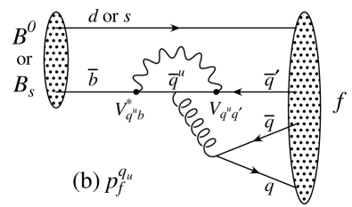
Figure 1: Feynman diagrams for (a) tree and (b) penguin amplitudes contributing to $B^{0}\to f$ or $B_{s}\to f$ via a $\bar{b}\to\bar{q}q\bar{q}^{\prime}$ quark-level process.

The $B^{0}\to J/\psi K^{0}$ decay [3, 4] proceeds via the quark transition $\bar{b}\to\bar{c}c\bar{s}$. There are contributions from both tree ($t$) and penguin ($p^{q_{u}}$, where $q_{u}=u,c,t$ is the quark in the loop) diagrams (see Fig. 1) which carry different weak phases:

$$A_{f}=\left(V^{\ast}_{cb}V_{cs}\right)t_{f}+\sum_{q_{u}=u,c,t}\left(V^{\ast}_{q_{u}b}V_{q_{u}s}\right)p^{q_{u}}_{f}\;.$$ (28)

(The distinction between tree and penguin contributions is a heuristic one, the separation by the operator that enters is more precise. For a detailed discussion of the more complete operator product approach, which also includes higher order QCD corrections, see, for example, ref. [5].) Using CKM unitarity, these decay amplitudes can always be written in terms of just two CKM combinations:

$$A_{\psi K}=\left(V^{\ast}_{cb}V_{cs}\right)T_{\psi K}+\left(V^{\ast}_{ub}V_{us}\right)P^{u}_{\psi K},$$ (29)

where $T_{\psi K}=t_{\psi K}+p^{c}_{\psi K}-p^{t}_{\psi K}$ and $P^{u}_{\psi K}=p^{u}_{\psi K}-p^{t}_{\psi K}$. A subtlety arises in this decay that is related to the fact that ${B}^{0}\to J/\psi K^{0}$ and $\overline{B}^{0}\to J/\psi\overline{K}{}^{0}$. A common final state, e.g. $J/\psi K_{S}$, can be reached via $K^{0}-\overline{K}{}^{0}$ mixing. Consequently, the phase factor corresponding to neutral $K$ mixing, $e^{-i\phi_{K}}=(V^{*}_{cd}V_{cs})/(V_{cd}V^{*}_{cs})$, plays a role:

$$\frac{\overline{A}_{\psi K_{S}}}{A_{\psi K_{S}}}=-\frac{\left(V_{cb}V^{\ast}_{cs}\right)T_{\psi K}+\left(V_{ub}V^{\ast}_{us}\right)P^{u}_{\psi K}}{\left(V^{\ast}_{cb}V_{cs}\right)T_{\psi K}+\left(V^{\ast}_{ub}V_{us}\right)P^{u}_{\psi K}}\times\frac{V_{cd}^{\ast}V_{cs}}{V_{cd}V_{cs}^{\ast}}.$$ (30)

The crucial point is that, for $B\to J/\psi K_{S}$ and other $\bar{b}\to\bar{c}c\bar{s}$ processes, we can neglect the $P^{u}$ contribution to $A_{\psi K}$, in the SM, to an approximation that is better than one percent:

$$|P^{u}_{\psi K}/T_{\psi K}|\times|V_{ub}/V_{cb}|\times|V_{us}/V_{cs}|\sim({\rm loop\ factor})\times 0.1\times 0.23\mathrel{\hbox to0.0pt{\lower 4.0pt\hbox{\hskip 1.0pt$\sim$}\hss}\raise 1.0pt\hbox{$<$}}0.005.$$ (31)

Thus, to an accuracy better than one percent,

$$\lambda_{\psi K_{S}}=\left(\frac{V_{tb}^{*}V_{td}}{V_{tb}V_{td}^{*}}\right)\left(\frac{V_{cb}V_{cd}^{*}}{V_{cb}^{*}V_{cd}}\right)=-e^{-2i\beta},$$ (32)

where $\beta$ is defined in Eq. (105), and consequently

$$S_{\psi K_{S}}=\sin 2\beta,\ \ \ C_{\psi K_{S}}=0\;.$$ (33)

(Below the percent level, several effects modify this equation [6, 7, 8, 9].)

Exercise 3: Show that, if the $B\to\pi\pi$ decays were dominated by tree diagrams, then $S_{\pi\pi}=\sin 2\alpha$.

Exercise 4: Estimate the accuracy of the predictions $S_{\phi K_{S}}=\sin 2\beta$ and $C_{\phi K_{S}}=0$.

When we consider extensions of the SM, we still do not expect any significant new contribution to the tree level decay, $b\to c\bar{c}s$, beyond the SM $W$-mediated diagram. Thus, the expression $\bar{A}_{\psi K_{S}}/A_{\psi K_{S}}=(V_{cb}V_{cd}^{*})/(V_{cb}^{*}V_{cd})$ remains valid, though the approximation of neglecting sub-dominant phases can be somewhat less accurate than Eq. (31). On the other hand, $M_{12}$, the $B^{0}-\overline{B}^{0}$ mixing amplitude, can in principle get large and even dominant contributions from new physics. We can parametrize the modification to the SM in terms of two parameters, $r_{d}^{2}$ signifying the change in magnitude, and $2\theta_{d}$ signifying the change in phase:

$$M_{12}=r_{d}^{2}\ e^{2i\theta_{d}}\ M_{12}^{\rm SM}(\rho,\eta).$$ (34)

This leads to the following generalization of Eq. (33):

$$S_{\psi K_{S}}=\sin(2\beta+2\theta_{d}),\ \ \ C_{\psi K_{S}}=0\;.$$ (35)

The experimental measurements give the following ranges [10]:

$$S_{\psi K_{S}}=+0.68\pm 0.02,\ \ \ C_{\psi K_{S}}=+0.005\pm 0.017\;.$$ (36)

0.4.2 Self-consistency of the CKM assumption

The three generation standard model has room for CP violation, through the KM phase in the quark mixing matrix. Yet, one would like to make sure that indeed CP is violated by the SM interactions, namely that $\sin\delta_{\rm KM}\neq 0$. If we establish that this is the case, we would further like to know whether the SM contributions to CP violating observables are dominant. More quantitatively, we would like to put an upper bound on the ratio between the new physics and the SM contributions.

As a first step, one can assume that flavor changing processes are fully described by the SM, and check the consistency of the various measurements with this assumption. There are four relevant mixing parameters, which can be taken to be the Wolfenstein parameters $\lambda$, $A$, $\rho$ and $\eta$ defined in Eq. (100). The values of $\lambda$ and $A$ are known rather accurately [11] from, respectively, $K\to\pi\ell\nu$ and $b\to c\ell\nu$ decays:

$$\lambda=0.2254\pm 0.0007,\ \ \ A=0.811^{+0.022}_{-0.012}.$$ (37)

Then, one can express all the relevant observables as a function of the two remaining parameters, $\rho$ and $\eta$, and check whether there is a range in the $\rho-\eta$ plane that is consistent with all measurements. The list of observables includes the following:

• The rates of inclusive and exclusive charmless semileptonic $B$ decays depend on $|V_{ub}|^{2}\propto\rho^{2}+\eta^{2}$;

• The CP asymmetry in $B\to\psi K_{S}$, $S_{\psi K_{S}}=\sin 2\beta=\frac{2\eta(1-\rho)}{(1-\rho)^{2}+\eta^{2}}$;

• The rates of various $B\to DK$ decays depend on the phase $\gamma$, where $e^{i\gamma}=\frac{\rho+i\eta}{\sqrt{\rho^{2}+\eta^{2}}}$;

• The rates of various $B\to\pi\pi,\rho\pi,\rho\rho$ decays depend on the phase $\alpha=\pi-\beta-\gamma$;

• The ratio between the mass splittings in the neutral $B$ and $B_{s}$ systems is sensitive to $|V_{td}/V_{ts}|^{2}=\lambda^{2}[(1-\rho)^{2}+\eta^{2}]$;

• The CP violation in $K\to\pi\pi$ decays, $\epsilon_{K}$, depends in a complicated way on $\rho$ and $\eta$.

The resulting constraints are shown in Fig. 2.

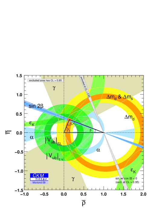
Figure 2: Allowed region in the $\rho,\eta$ plane. Superimposed are the individual constraints from charmless semileptonic $B$ decays ($|V_{ub}/V_{cb}|$), mass differences in the $B^{0}$ ($\Delta m_{d}$) and $B_{s}$ ($\Delta m_{s}$) neutral meson systems, and CP violation in $K\to\pi\pi$ ($\varepsilon_{K}$), $B\to\psi K$ ($\sin 2\beta$), $B\to\pi\pi,\rho\pi,\rho\rho$ ($\alpha$), and $B\to DK$ ($\gamma$). Taken from [12].

The consistency of the various constraints is impressive. In particular, the following ranges for $\rho$ and $\eta$ can account for all the measurements [11]:

$$\rho=+0.131^{+0.026}_{-0.013},\ \ \ \eta=+0.345\pm 0.014.$$ (38)

One can make then the following statement [13]:
Very likely, CP violation in flavor changing processes is dominated by the Kobayashi-Maskawa phase.

In the next two subsections, we explain how we can remove the phrase “very likely” from this statement, and how we can quantify the KM-dominance.

0.4.3 Is the KM mechanism at work?

In proving that the KM mechanism is at work, we assume that charged-current tree-level processes are dominated by the $W$-mediated SM diagrams (see, for example, [14]). This is a very plausible assumption. I am not aware of any viable well-motivated model where this assumption is not valid. Thus we can use all tree level processes and fit them to $\rho$ and $\eta$, as we did before. The list of such processes includes the following:

1. Charmless semileptonic $B$-decays, $b\to u\ell\nu$, measure $R_{u}$ [see Eq. (104)].

2. $B\to DK$ decays, which go through the quark transitions $b\to c\bar{u}s$ and $b\to u\bar{c}s$, measure the angle $\gamma$ [see Eq. (105)].

3. $B\to\rho\rho$ decays (and, similarly, $B\to\pi\pi$ and $B\to\rho\pi$ decays) go through the quark transition $b\to u\bar{u}d$. With an isospin analysis, one can determine the relative phase between the tree decay amplitude and the mixing amplitude. By incorporating the measurement of $S_{\psi K_{S}}$, one can subtract the phase from the mixing amplitude, finally providing a measurement of the angle $\gamma$ [see Eq. (105)].

In addition, we can use loop processes, but then we must allow for new physics contributions, in addition to the $(\rho,\eta)$-dependent SM contributions. Of course, if each such measurement adds a separate mode-dependent parameter, then we do not gain anything by using this information. However, there is a number of observables where the only relevant loop process is $B^{0}-\overline{B}{}^{0}$ mixing. The list includes $S_{\psi K_{S}}$, $\Delta m_{B}$ and the CP asymmetry in semileptonic $B$ decays:

$$S_{\psi K_{S}} = \sin(2\beta+2\theta_{d}),$$

$$\Delta m_{B} = r_{d}^{2}(\Delta m_{B})^{\rm SM},$$

$${\cal A}_{\rm SL} = -{\cal R}e\left(\frac{\Gamma_{12}}{M_{12}}\right)^{\rm SM}\frac{\sin 2\theta_{d}}{r_{d}^{2}}+{\cal I}m\left(\frac{\Gamma_{12}}{M_{12}}\right)^{\rm SM}\frac{\cos 2\theta_{d}}{r_{d}^{2}}.$$ (39)

As explained above, such processes involve two new parameters [see Eq. (34)]. Since there are three relevant observables, we can further tighten the constraints in the $(\rho,\eta)$-plane. Similarly, one can use measurements related to $B_{s}-\overline{B}_{s}$ mixing. One gains three new observables at the cost of two new parameters (see, for example, [15]).

The results of such fit, projected on the $\rho-\eta$ plane, can be seen in Fig. 3. It gives [12]

$$\eta=0.44^{+0.05}_{-0.23}\ \ (3\sigma).$$ (40)

[A similar analysis in Ref. [16] obtains the $3\sigma$ range $(0.31-0.46)$.] It is clear that $\eta\neq 0$ is well established:
The Kobayashi-Maskawa mechanism of CP violation is at work.

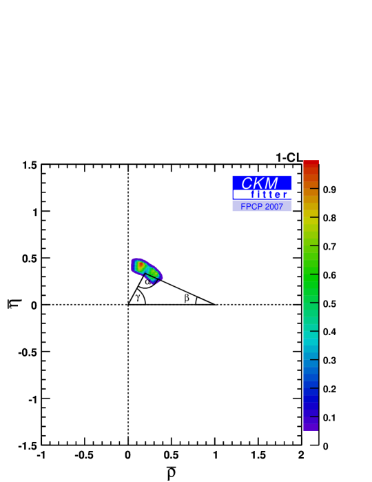
Figure 3: The allowed region in the $\rho-\eta$ plane, assuming that tree diagrams are dominated by the Standard Model [12].

Another way to establish that CP is violated by the CKM matrix is to find, within the same procedure, the allowed range for $\sin 2\beta$ [16]:

$$\sin 2\beta^{\rm tree}=0.80\pm 0.03.$$ (41)

Thus, $\beta\neq 0$ is well established.

The consistency of the experimental results (36) with the SM predictions (33,41) means that the KM mechanism of CP violation dominates the observed CP violation. In the next subsection, we make this statement more quantitative.

0.4.4 How much can new physics contribute to $B^{0}-\overline{B}{}^{0}$ mixing?

All that we need to do in order to establish whether the SM dominates the observed CP violation, and to put an upper bound on the new physics contribution to $B^{0}-\overline{B}{}^{0}$ mixing, is to project the results of the fit performed in the previous subsection on the $r_{d}^{2}-2\theta_{d}$ plane. If we find that $\theta_{d}\ll\beta$, then the SM dominance in the observed CP violation will be established. The constraints are shown in Fig. 4(a). Indeed, $\theta_{d}\ll\beta$.

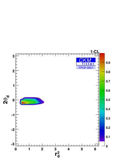
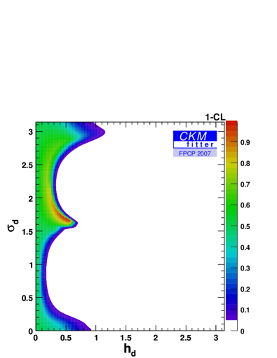
Figure 4: Constraints in the (a) $r_{d}^{2}-2\theta_{d}$ plane, and (b) $h_{d}-\sigma_{d}$ plane, assuming that NP contributions to tree level processes are negligible [12].

An alternative way to present the data is to use the $h_{d},\sigma_{d}$ parametrization,

$$r_{d}^{2}e^{2i\theta_{d}}=1+h_{d}e^{2i\sigma_{d}}.$$ (42)

While the $r_{d},\theta_{d}$ parameters give the relation between the full mixing amplitude and the SM one, and are convenient to apply to the measurements, the $h_{d},\sigma_{d}$ parameters give the relation between the new physics and SM contributions, and are more convenient in testing theoretical models:

$$h_{d}e^{2i\sigma_{d}}=\frac{M_{12}^{\rm NP}}{M_{12}^{\rm SM}}.$$ (43)

The constraints in the $h_{d}-\sigma_{d}$ plane are shown in Fig. 4(b). We can make the following two statements:

1. A new physics contribution to $B^{0}-\overline{B}^{0}$ mixing amplitude that carries a phase that is significantly different from the KM phase is constrained to lie below the 20-30% level.

2. A new physics contribution to the $B^{0}-\overline{B}^{0}$ mixing amplitude which is aligned with the KM phase is constrained to be at most comparable to the CKM contribution.

One can reformulate these statements as follows:

1. The KM mechanism dominates CP violation in $B^{0}-\overline{B}^{0}$ mixing.

2. The CKM mechanism is a major player in $B^{0}-\overline{B}^{0}$ mixing.

0.5 The new physics flavor puzzle

0.5.1 A model independent discussion

It is clear that the Standard Model is not a complete theory of Nature:

1. It does not include gravity, and therefore it cannot be valid at energy scales above $m_{\rm Planck}\sim 10^{19}$ GeV:

2. It does not allow for neutrino masses, and therefore it cannot be valid at energy scales above $m_{\rm seesaw}\sim 10^{15}$ GeV;

3. The fine-tuning problem of the Higgs mass suggests that the scale where the SM is replaced with a more fundamental theory is actually much lower, $m_{\rm top-partners}\mathrel{\hbox to0.0pt{\lower 4.0pt\hbox{\hskip 1.0pt$\sim$}\hss}\raise 1.0pt\hbox{$<$}}$ a few TeV.

4. If the dark matter is made of weakly interacting massive particles (WIMPs) then, again, a low scale of new physics is likely, $m_{\rm wimp}\mathrel{\hbox to0.0pt{\lower 4.0pt\hbox{\hskip 1.0pt$\sim$}\hss}\raise 1.0pt\hbox{$<$}}$ a few TeV.

Given that the SM is only an effective low energy theory, non-renormalizable terms must be added to ${\cal L}_{\rm SM}$ of Eq. (4). These are terms of dimension higher than four in the fields which, therefore, have couplings that are inversely proportional to the scale of new physics $\Lambda_{\rm NP}$. For example, the lowest dimension non-renormalizable terms are dimension five:

$$-{\cal L}_{\rm Yukawa}^{\rm dim-5}={Z_{ij}^{\nu}\over\Lambda_{\rm NP}}L_{Li}^{I}L_{Lj}^{I}\phi\phi+{\rm h.c.}.$$ (44)

These are the seesaw terms, leading to neutrino masses.

Exercise 5: How does the global symmetry breaking pattern (14) change when (44) is taken into account?

Exercise 6: What is the number of physical lepton flavor parameters in this case? Identify these parameters in the mass basis.

As concerns quark flavor physics, consider, for example, the following dimension-six, four-fermion, flavor changing operators:

$${\cal L}_{\Delta F=2}=\frac{z_{sd}}{\Lambda_{\rm NP}^{2}}(\overline{d_{L}}\gamma_{\mu}s_{L})^{2}+\frac{z_{cu}}{\Lambda_{\rm NP}^{2}}(\overline{c_{L}}\gamma_{\mu}u_{L})^{2}+\frac{z_{bd}}{\Lambda_{\rm NP}^{2}}(\overline{d_{L}}\gamma_{\mu}b_{L})^{2}+\frac{z_{bs}}{\Lambda_{\rm NP}^{2}}(\overline{s_{L}}\gamma_{\mu}b_{L})^{2}.$$ (45)

Each of these terms contributes to the mass splitting between the corresponding two neutral mesons. For example, the term ${\cal L}_{\Delta B=2}\propto(\overline{d_{L}}\gamma_{\mu}b_{L})^{2}$ contributes to $\Delta m_{B}$, the mass difference between the two neutral $B$-mesons. We use $M_{12}^{B}=\frac{1}{2m_{B}}\langle B^{0}|{\cal L}_{\Delta F=2}|\overline{B}^{0}\rangle$ and

$$\langle B^{0}|(\overline{d_{La}}\gamma^{\mu}b_{La})(\overline{d_{Lb}}\gamma_{\mu}b_{Lb})|\overline{B}^{0}\rangle=-\frac{1}{3}m_{B}^{2}f_{B}^{2}B_{B}.$$ (46)

This leads to $\Delta m_{B}/m_{B}=2|M_{12}^{B}|/m_{B}\sim(|z_{bd}|/3)(f_{B}/\Lambda_{\rm NP})^{2}$. Analogous expressions hold for the other neutral mesons.

The experimental results for CP conserving and CP violating observables related to neutral meson mixing (mass splittings and CP asymmetries in tree level decays, respectively) are given in Table 1.

Table 1: Measurements related to neutral meson mixing

Sector	CP-conserving	CP-violating
sd	$\Delta m_{K}/m_{K}=7.0\times 10^{-15}$	$\epsilon_{K}=2.3\times 10^{-3}$
cu	$\Delta m_{D}/m_{D}=8.7\times 10^{-15}$	$A_{\Gamma}/y_{\rm CP}\mathrel{\hbox to0.0pt{\lower 4.0pt\hbox{\hskip 1.0pt$\sim$}\hss}\raise 1.0pt\hbox{$<$}}0.2$
bd	$\Delta m_{B}/m_{B}=6.3\times 10^{-14}$	$S_{\psi K}=+0.67\pm 0.02$
bs	$\Delta m_{B_{s}}/m_{B_{s}}=2.1\times 10^{-12}$	$S_{\psi\phi}=-0.04\pm 0.09$

The measurements quoted in Table 1 lead, for a given value of $|z_{ij}|$ and $z^{I}_{ij}\equiv{\cal I}m(z_{ij})$, to lower bounds on the scale $\Lambda_{\rm NP}$. In Table 2 we give the bounds that correspond to $|z_{ij}|=1$ and to $z^{I}_{ij}=1$. The bounds scale like $\sqrt{z_{ij}}$ and $\sqrt{z^{I}_{ij}}$, respectively.

Table 2: Lower bounds on the scale of new physics $\Lambda_{\rm NP}$, in units of TeV. The bounds from CP conserving (violating) observables scale like $\sqrt{z_{ij}}$ ($\sqrt{z^{I}_{ij}}$).

$ij$	CP-conserving	CP-violating
sd	$1\times 10^{3}$	$2\times 10^{4}$
cu	$1\times 10^{3}$	$3\times 10^{3}$
bd	$4\times 10^{2}$	$8\times 10^{2}$
bs	$7\times 10^{1}$	$2\times 10^{2}$

We conclude that if the new physics has a generic flavor structure, that is $z_{ij}={\cal O}(1)$, then its scale must be above $10^{3}-10^{4}$ TeV. If the leading contributions involve electroweak loops, the lower bound is somewhat lower, of order $10^{2}-10^{3}$ TeV. The bounds from the corresponding four-fermi terms with LR structure, instead of the LL structure of Eq. (45), are even stronger. If indeed $\Lambda_{\rm NP}\gg TeV$, it means that we have misinterpreted the hints from the fine-tuning problem and the dark matter puzzle.

There is, however, another way to look at these constraints:

$$z_{sd} \mathrel{\hbox to0.0pt{\lower 4.0pt\hbox{\hskip 1.0pt$\sim$}\hss}\raise 1.0pt\hbox{$<$}} 8\times 10^{-7}\ (\Lambda_{\rm NP}/TeV)^{2},$$

$$z_{cu} \mathrel{\hbox to0.0pt{\lower 4.0pt\hbox{\hskip 1.0pt$\sim$}\hss}\raise 1.0pt\hbox{$<$}} 5\times 10^{-7}\ (\Lambda_{\rm NP}/TeV)^{2},$$

$$z_{bd} \mathrel{\hbox to0.0pt{\lower 4.0pt\hbox{\hskip 1.0pt$\sim$}\hss}\raise 1.0pt\hbox{$<$}} 5\times 10^{-6}\ (\Lambda_{\rm NP}/TeV)^{2},$$

$$z_{bs} \mathrel{\hbox to0.0pt{\lower 4.0pt\hbox{\hskip 1.0pt$\sim$}\hss}\raise 1.0pt\hbox{$<$}} 2\times 10^{-4}\ (\Lambda_{\rm NP}/TeV)^{2},$$ (47)

$$z_{sd}^{I} \mathrel{\hbox to0.0pt{\lower 4.0pt\hbox{\hskip 1.0pt$\sim$}\hss}\raise 1.0pt\hbox{$<$}} 6\times 10^{-9}\ (\Lambda_{\rm NP}/TeV)^{2},$$

$$z_{cu}^{I} \mathrel{\hbox to0.0pt{\lower 4.0pt\hbox{\hskip 1.0pt$\sim$}\hss}\raise 1.0pt\hbox{$<$}} 1\times 10^{-7}\ (\Lambda_{\rm NP}/TeV)^{2},$$

$$z_{bd}^{I} \mathrel{\hbox to0.0pt{\lower 4.0pt\hbox{\hskip 1.0pt$\sim$}\hss}\raise 1.0pt\hbox{$<$}} 1\times 10^{-6}\ (\Lambda_{\rm NP}/TeV)^{2},$$

$$z_{bs}^{I} \mathrel{\hbox to0.0pt{\lower 4.0pt\hbox{\hskip 1.0pt$\sim$}\hss}\raise 1.0pt\hbox{$<$}} 2\times 10^{-5}\ (\Lambda_{\rm NP}/TeV)^{2}.$$ (48)

It could be that the scale of new physics is of order TeV, but its flavor structure is far from generic. Specifically, if new particles at the TeV scale couple to the SM fermions, then there are two ways in which their contributions to FCNC processes, such as neutral meson mixing, can be suppressed: degeneracy and alignment. Either of these principles, or a combination of both, signifies non-generic structure.

One can use the language of effective operators also for the SM, integrating out all particles significantly heavier than the neutral mesons (that is, the top, the Higgs and the weak gauge bosons). Thus, the scale is $\Lambda_{\rm SM}\sim m_{W}$. Since the leading contributions to neutral meson mixings come from box diagrams, the $z_{ij}$ coefficients are suppressed by $\alpha_{2}^{2}$. To identify the relevant flavor suppression factor, one can employ the spurion formalism. For example, the flavor transition that is relevant to $B^{0}-\overline{B}{}^{0}$ mixing involves $\overline{d_{L}}b_{L}$ which transforms as $(8,1,1)_{SU(3)_{q}^{3}}$. The leading contribution must then be proportional to $(Y^{u}Y^{u\dagger})_{13}\propto y_{t}^{2}V_{tb}V_{td}^{*}$. Indeed, an explicit calculation, using VIA for the matrix element and neglecting QCD corrections, gives (a detailed derivation can be found in Appendix B of [17])

$$\frac{2M_{12}^{B}}{m_{B}}\approx-\frac{\alpha_{2}^{2}}{12}\frac{f_{B}^{2}}{m_{W}^{2}}S_{0}(x_{t})(V_{tb}V_{td}^{*})^{2},$$ (49)

where $x_{i}=m_{i}^{2}/m_{W}^{2}$ and

$$S_{0}(x)=\frac{x}{(1-x)^{2}}\left[1-\frac{11x}{4}+\frac{x^{2}}{4}-\frac{3x^{2}\ln x}{2(1-x)}\right].$$ (50)

Similar spurion analyses, or explicit calculations, allow us to extract the weak and flavor suppression factors that apply in the SM:

$${\cal I}m(z_{sd}^{\rm SM}) \sim \alpha_{2}^{2}y_{t}^{2}|V_{td}V_{ts}|^{2}\sim 1\times 10^{-10},$$

$$z_{sd}^{\rm SM} \sim \alpha_{2}^{2}y_{c}^{2}|V_{cd}V_{cs}|^{2}\sim 5\times 10^{-9},$$

$${\cal I}m(z_{cu}^{\rm SM}) \sim \alpha_{2}^{2}y_{b}^{2}|V_{ub}V_{cb}|^{2}\sim 2\times 10^{-14},$$

$$z_{bd}^{\rm SM} \sim \alpha_{2}^{2}y_{t}^{2}|V_{td}V_{tb}|^{2}\sim 7\times 10^{-8},$$

$$z_{bs}^{\rm SM} \sim \alpha_{2}^{2}y_{t}^{2}|V_{ts}V_{tb}|^{2}\sim 2\times 10^{-6}.$$ (51)

Note that we did not include $z_{cu}^{\rm SM}$ in the list. The reason is tha it requires a more detailed consideration. The naively leading short distance contribution is $\propto\alpha_{2}^{2}(y_{s}^{4}/y_{c}^{2})|V_{cs}V_{us}|^{2}\sim 5\times 10^{-13}$. However, higher dimension terms can replace a $y_{s}^{2}$ factor with $(\Lambda/m_{D})^{2}$ [18]. Moreover, long distance contributions are expected to dominate. In particular, peculiar phase space effects [19, 20] have been identified which are expected to enhance $\Delta m_{D}$ to within an order of magnitude of the its measured value. The CP violating part, on the other hand, is dominated by short distance physics.

It is clear then that contributions from new physics at $\Lambda_{\rm NP}\sim 1\ TeV$ should be suppressed by factors that are comparable or smaller than the SM ones. Why does that happen? This is the new physics flavor puzzle.

The fact that the flavor structure of new physics at the TeV scale must be non-generic means that flavor measurements are a good probe of the new physics. Perhaps the best-studied example is that of supersymmetry. Here, the spectrum of the superpartners and the structure of their couplings to the SM fermions will allow us to probe the mechanism of dynamical supersymmetry breaking.

0.5.2 The supersymmetric flavor puzzle

We consider, as an example, the contributions from the box diagrams involving the squark doublets of the second and third generations, $\tilde{Q}_{L2,3}$, to the $B_{s}-\overline{B_{s}}$ mixing amplitude. The contributions are proportional to $K_{3i}^{d*}K^{d}_{2i}K_{3j}^{d*}K^{d}_{2j}$, where $K^{d}$ is the mixing matrix of the gluino couplings to a left-handed down quark and their supersymmetric squark partners ($\propto[(\delta^{d}_{LL})_{23}]^{2}$ in the mass insertion approximation, described in Appendix .11.1). We work in the mass basis for both quarks and squarks. A detailed derivation [21] is given in Appendix .11.2. It gives:

$$M_{12}^{s} = \frac{\alpha_{s}^{2}m_{B_{s}}f_{B_{s}}^{2}B_{B_{s}}\eta_{\rm QCD}}{108m_{\tilde{d}}^{2}}[11\tilde{f}_{6}(x)+4xf_{6}(x)]\frac{(\Delta\tilde{m}^{2}_{\tilde{d}})^{2}}{\tilde{m}_{d}^{4}}(K_{32}^{d*}K_{22}^{d})^{2}.$$ (52)

Here $m_{\tilde{d}}$ is the average mass of the two squark generations, $\Delta m^{2}_{\tilde{d}}$ is the mass-squared difference, and $x=m_{\tilde{g}}^{2}/m_{\tilde{d}}^{2}$.

Eq. (52) can be translated into our generic language:

$$\Lambda_{\rm NP} = m_{\tilde{q}},$$ (53)

$$z_{1}^{bs} = \frac{11\tilde{f}_{6}(x)+4xf_{6}(x)}{18}\alpha_{s}^{2}\left(\frac{\Delta\tilde{m}_{\tilde{d}}^{2}}{m_{\tilde{d}}^{2}}\right)^{2}(K_{32}^{d*}K_{22}^{d})^{2}\approx 10^{-4}(\delta^{LL}_{23})^{2},$$

where, for the last approximation, we took the example of $x=1$ [and used, correspondingly, $11\tilde{f}_{6}(1)+4f_{6}(1)=1/6$], and defined

$$\delta^{LL}_{23}=\left(\frac{\Delta\tilde{m}_{\tilde{d}}^{2}}{m_{\tilde{d}}^{2}}\right)(K_{32}^{d*}K_{22}^{d}).$$ (54)

Similar expressions can be derived for the dependence of $K^{0}-\overline{K^{0}}$ on $(\delta^{d}_{MN})_{12}$, $B^{0}-\overline{B^{0}}$ on $(\delta^{d}_{MN})_{13}$, and $D^{0}-\overline{D^{0}}$ on $(\delta^{u}_{MN})_{12}$. Then we can use the constraints of Eqs. (0.5.1,0.5.1) to put upper bounds on $(\delta^{q}_{MN})_{ij}$. Some examples are given in Table 3 (see Ref. [22] for details and list of references).

Table 3: The phenomenological upper bounds on $(\delta^{q}_{LL})_{ij}$ and $\langle\delta^{q}_{ij}\rangle=\sqrt{(\delta^{q}_{LL})_{ij}(\delta^{q}_{RR})_{ij}}$. Here $q=u,d$ and $M=L,R$. The constraints are given for $m_{\tilde{q}}=1$ TeV and $x=m_{\tilde{g}}^{2}/m_{\tilde{q}}^{2}=1$. We assume that the phases could suppress the imaginary part by a factor of $\sim 0.3$. Taken from Ref. [22].

$q$	$ij$	$(\delta^{q}_{LL})_{ij}$	$\langle\delta^{q}_{ij}\rangle$
d	12	0.03	0.002
d	13	0.2	0.07
d	23	0.2	0.07
u	12	0.1	0.008

We learn that, in most cases, we need $\delta^{q}_{ij}/m_{\tilde{q}}\ll 1/{\rm TeV}$. One can immediately identify three generic ways in which supersymmetric contributions to neutral meson mixing can be suppressed:

1. Heaviness: $m_{\tilde{q}}\gg 1\ TeV$;

2. Degeneracy: $\Delta m^{2}_{\tilde{q}}\ll m_{\tilde{q}}^{2}$;

3. Alignment: $K^{q}_{ij}\ll 1$.

When heaviness is the only suppression mechanism, as in split supersymmetry [23], the squarks are very heavy and supersymmetry no longer solves the fine tuning problem. (When the first two squark generations are mildly heavy and the third generation is light, as in effective supersymmetry [24], the fine tuning problem is still solved, but additional suppression mechanisms are needed.) If we want to maintain supersymmetry as a solution to the fine tuning problem, either degeneracy or alignment or a combination of the two is needed. This means that the flavor structure of supersymmetry is not generic, as argued in the previous section.

Take, for example, $(\delta^{d}_{LL})_{12}\leq 0.03$. Naively, one might expect the alignment to be of order $(V_{cd}V_{cs}^{*})\sim 0.2$, which is far from sufficient by itself. Barring a very precise alignment ($|K^{d}_{12}|\ll|V_{us}|$) [25, 26] and accidental cancelations, we are led to conclude that the first two squark generations must be quasi-degenerate. Actually, by combining the constraints from $K^{0}-\overline{K^{0}}$ mixing and $D^{0}-\overline{D^{0}}$ mixing, one can show that this is the case independently of assumptions about the alignment [27, 28, 29]. Analogous conclusions can be drawn for many TeV-scale new physics scenarios: a strong level of degeneracy is required (for definitions and detailed analysis, see [30]).

Exercise 9: Does $K_{31}^{d}\sim|V_{ub}|$ suffice to satisfy the $\Delta m_{B}$ constraint with neither degeneracy nor heaviness? (Use the two generation approximation and ignore the second generation.)

Is there a natural way to make the squarks degenerate? Degeneracy requires that the $3\times 3$ matrix of soft supersymmetry breaking mass-squared terms $\tilde{m}^{2}_{Q_{L}}\simeq\tilde{m}^{2}_{\tilde{q}}{\bf 1}$. We have mentioned already that flavor universality is a generic feature of gauge interactions. Thus, the requirement of degeneracy is perhaps a hint that supersymmetry breaking is gauge mediated to the MSSM fields.

0.5.3 Minimal flavor violation (MFV)

If supersymmetry breaking is gauge mediated, the squark mass matrices for $SU(2)_{L}$- doublet and $SU(2)_{L}$-singlet squarks have the following form at the scale of mediation $m_{M}$:

$$\tilde{M}^{2}_{U_{L}}(m_{M}) = \left(m^{2}_{\tilde{Q}_{L}}+D_{U_{L}}\right){\bf 1}+M_{u}M_{u}^{\dagger},$$

$$\tilde{M}^{2}_{D_{L}}(m_{M}) = \left(m^{2}_{\tilde{Q}_{L}}+D_{D_{L}}\right){\bf 1}+M_{d}M_{d}^{\dagger},$$

$$\tilde{M}^{2}_{U_{R}}(m_{M}) = \left(m^{2}_{\tilde{U}_{R}}+D_{U_{R}}\right){\bf 1}+M_{u}^{\dagger}M_{u},$$

$$\tilde{M}^{2}_{D_{R}}(m_{M}) = \left(m^{2}_{\tilde{D}_{R}}+D_{D_{R}}\right){\bf 1}+M_{d}^{\dagger}M_{d},$$ (55)

where $D_{q_{A}}=(T_{3})_{q_{A}}-(Q_{\rm EM})_{q_{A}}s^{2}_{W}m_{Z}^{2}\cos 2\beta$ are the $D$-term contributions. Here, the only source of the $SU(3)^{3}_{q}$ breaking are the SM Yukawa matrices.

This statement holds also when the renormalization group evolution is applied to find the form of these matrices at the weak scale. Taking the scale of the soft breaking terms $m_{\tilde{q}_{A}}$ to be somewhat higher than the electroweak breaking scale $m_{Z}$ allows us to neglect the $D_{q_{A}}$ and $M_{q}$ terms in (0.5.3). Then we obtain

$$\tilde{M}^{2}_{Q_{L}}(m_{Z}) \sim m^{2}_{\tilde{Q}_{L}}\left(r_{3}{\bf 1}+c_{u}Y_{u}Y_{u}^{\dagger}+c_{d}Y_{d}Y_{d}^{\dagger}\right),$$

$$\tilde{M}^{2}_{U_{R}}(m_{Z}) \sim m^{2}_{\tilde{U}_{R}}\left(r_{3}{\bf 1}+c_{uR}Y_{u}^{\dagger}Y_{u}\right),$$

$$\tilde{M}^{2}_{D_{R}}(m_{Z}) \sim m^{2}_{\tilde{D}_{R}}\left(r_{3}{\bf 1}+c_{dR}Y_{d}^{\dagger}Y_{d}\right).$$ (56)

Here $r_{3}$ represents the universal RGE contribution that is proportional to the gluino mass ($r_{3}={\cal O}(6)\times(M_{3}(m_{M})/m_{\tilde{q}}(m_{M}))$) and the $c$-coefficients depend logarithmically on $m_{M}/m_{Z}$ and can be of ${\cal O}(1)$ when $m_{M}$ is not far below the GUT scale.

Models of gauge mediated supersymmetry breaking (GMSB) provide a concrete example of a large class of models that obey a simple principle called minimal flavor violation (MFV) [31]. This principle guarantees that low energy flavor changing processes deviate only very little from the SM predictions. The basic idea can be described as follows. The gauge interactions of the SM are universal in flavor space. The only breaking of this flavor universality comes from the three Yukawa matrices, $Y^{u}$, $Y^{d}$ and $Y^{e}$. If this remains true in the presence of the new physics, namely $Y^{u}$, $Y^{d}$ and $Y^{e}$ are the only flavor non-universal parameters, then the model belongs to the MFV class.

Let us now formulate this principle in a more formal way, using the language of spurions that we presented in section 0.3.2. The Standard Model with vanishing Yukawa couplings has a large global symmetry (11,0.3.2). In this section we concentrate only on the quarks. The non-Abelian part of the flavor symmetry for the quarks is $SU(3)_{q}^{3}$ of Eq. (0.3.2) with the three generations of quark fields transforming as follows:

$$Q_{L}(3,1,1),\ \ U_{R}(1,3,1),\ \ D_{R}(1,1,3).$$ (57)

The Yukawa interactions,

$${\cal L}_{Y}=\overline{Q_{L}}Y^{d}D_{R}H+\overline{Q_{L}}Y^{u}U_{R}H_{c},$$ (58)

($H_{c}=i\tau_{2}H^{*}$) break this symmetry. The Yukawa couplings can thus be thought of as spurions with the following transformation properties under $SU(3)_{q}^{3}$ [see Eq. (15)]:

$$Y^{u}\sim(3,\bar{3},1),\qquad Y^{d}\sim(3,1,\bar{3}).$$ (59)

When we say “spurions”, we mean that we pretend that the Yukawa matrices are fields which transform under the flavor symmetry, and then require that all the Lagrangian terms, constructed from the SM fields, $Y^{d}$ and $Y^{u}$, must be (formally) invariant under the flavor group $SU(3)_{q}^{3}$. Of course, in reality, ${\cal L}_{Y}$ breaks $SU(3)_{q}^{3}$ precisely because $Y^{d,u}$ are not fields and do not transform under the symmetry.

The idea of minimal flavor violation is relevant to extensions of the SM, and can be applied in two ways:

1. If we consider the SM as a low energy effective theory, then all higher-dimension operators, constructed from SM-fields and $Y$-spurions, are formally invariant under $G_{\rm global}$.

2. If we consider a full high-energy theory that extends the SM, then all operators, constructed from SM and the new fields, and from $Y$-spurions, are formally invariant under $G_{\rm global}$.

Exercise 10: Use the spurion formalism to argue that, in MFV models, the $K_{L}\to\pi^{0}\nu\bar{\nu}$ decay amplitude is proportional to $y_{t}^{2}V_{td}V_{ts}^{*}$.

Exercise 11: Find the flavor suppression factors in the $z_{i}^{bs}$ coefficients, if MFV is imposed, and compare to the bounds in Eq. (0.5.1).

Examples of MFV models include models of supersymmetry with gauge-mediation or with anomaly-mediation of its breaking.

Testing MFV at the LHC

If the LHC discovers new particles that couple to the SM fermions, then it will be able to test solutions to the new physics flavor puzzle such as MFV [32]. Much of its power to test such frameworks is based on identifying top and bottom quarks.

To understand this statement, we notice that the spurions $Y^{u}$ and $Y^{d}$ can always be written in terms of the two diagonal Yukawa matrices $\lambda_{u}$ and $\lambda_{d}$ and the CKM matrix $V$, see Eqs. (17,18). Thus, the only source of quark flavor changing transitions in MFV models is the CKM matrix. Next, note that to an accuracy that is better than ${\cal O}(0.05)$, we can write the CKM matrix as follows:

$$V=\pmatrix{1}&0.230\\ -0.2310\\ 001\\ .$$ (60)

Exercise 12: The approximation (60) should be intuitively obvious to top-physicists, but definitely counter-intuitive to bottom-physicists. (Some of them have dedicated a large part of their careers to experimental or theoretical efforts to determine $V_{cb}$ and $V_{ub}$.) What does the approximation imply for the bottom quark? When we take into account that it is only good to ${\cal O}(0.05)$, what would the implications be?

We learn that the third generation of quarks is decoupled, to a good approximation, from the first two. This, in turn, means that any new particle that couples to an odd number of the SM quarks (think, for example, of heavy quarks in vector-like representations of $G_{\rm SM}$), decay into either third generation quark, or to non-third generation quark, but not to both. For example, in Ref. [32], MFV models with additional charge $-1/3$, $SU(2)_{\rm L}$-singlet quarks – $B^{\prime}$ – were considered. A concrete test of MFV was proposed, based on the fact that the largest mixing effect involving the third generation is of order $|V_{cb}|^{2}\sim 0.002$: Is the following prediction, concerning events of $B^{\prime}$ pair production, fulfilled:

$$\frac{\Gamma(B^{\prime}\overline{B^{\prime}}\to Xq_{1,2}q_{3})}{\Gamma(B^{\prime}\overline{B^{\prime}}\to Xq_{1,2}q_{1,2})+\Gamma(B^{\prime}\overline{B^{\prime}}\to Xq_{3}q_{3})}\mathrel{\hbox to0.0pt{\lower 4.0pt\hbox{\hskip 1.0pt$\sim$}\hss}\raise 1.0pt\hbox{$<$}}10^{-3}.$$ (61)

If not, then MFV is excluded. One could similarly test various versions of minimal lepton flavor violation (MLFV) [33, 34, 35, 36, 37, 38].

Analogous tests can be carried out in the supersymmetric framework [39, 43, 44, 40, 41, 42, 45]. Here, there is also a generic prediction that, in each of the three sectors ($Q_{L},U_{R},D_{R}$), squarks of the first two generations are quasi-degenerate, and do not decay into third generation quarks. Squarks of the third generation can be separated in mass (though, for small $\tan\beta$, the degeneracy in the $\tilde{D}_{R}$ sector is threefold), and decay only to third generation quarks.

We conclude that measurements at the LHC related to new particles that couple to the SM fermions are likely to teach us much more about flavor physics.

0.6 The Standard Model flavor puzzle

The SM has thirteen flavor parameters: six quark Yukawa couplings, four CKM parameters (three angles and a phase), and three charged lepton Yukawa couplings. (One can use fermions masses instead of the fermion Yukawa couplings, $Y_{f}=\sqrt{2}m_{f}/v$.) The orders of magnitudes of these thirteen dimensionless parameters are as follows:

$$Y_{t} \sim 1,\ \ \ Y_{c}\sim 10^{-2},\ \ \ Y_{u}\sim 10^{-5},$$

$$Y_{b} \sim 10^{-2},\ \ \ Y_{s}\sim 10^{-3},\ \ \ Y_{d}\sim 10^{-4},$$

$$Y_{\tau} \sim 10^{-2},\ \ \ Y_{\mu}\sim 10^{-3},\ \ \ Y_{e}\sim 10^{-6},$$

$$|V_{us}| \sim 0.2,\ \ |V_{cb}|\sim 0.04,\ \ |V_{ub}|\sim 0.004,\ \ \ \delta_{\rm KM}\sim 1.$$ (62)

Only two of these parameters are clearly of ${\cal O}(1)$, the top-Yukawa and the KM phase. The other flavor parameters exhibit smallness and hierarchy. Their values span six orders of magnitude. It may be that this set of numerical values are just accidental. More likely, the smallness and the hierarchy have a reason. The question of why there is smallness and hierarchy in the SM flavor parameters constitutes “The Standard Model flavor puzzle."

The motivation to think that there is indeed a structure in the flavor parameters is strengthened by considering the values of the four SM parameters that are not flavor parameters, namely the three gauge couplings and the Higgs self-coupling:

$$g_{s}\sim 1,\ \ g\sim 0.6,\ \ e\sim 0.3,\ \ \lambda\sim 0.2.$$ (63)

This set of values does seem to be a random distribution of order-one numbers, as one would naively expect.

A few examples of mechanisms that were proposed to explain the observed structure of the flavor parameters are the following:

• An approximate Abelian symmetry (“The Froggatt-Nielsen mechanism" [46]);

• An approximate non-Abelian symmetry (see e.g. [47]);

• Conformal dynamics (“The Nelson-Strassler mechanism" [48]);

• Location in an extra dimension [49].

We will take as an example the Froggatt-Nielsen mechanism.

0.6.1 The Froggatt-Nielsen mechanism

Small numbers and hierarchies are often explained by approximate symmetries. For example, the small mass splitting between the charged and neural pions finds an explanation in the approximate isospin (global $SU(2)$) symmetry of the strong interactions.

Approximate symmetries lead to selection rules which account for the size of deviations from the symmetry limit. Spurion analysis is particularly convenient to derive such selection rules. The Froggatt-Nielsen mechanism postulates a $U(1)_{H}$ symmetry, that is broken by a small spurion $\epsilon_{H}$. Without loss of generality, we assign $\epsilon_{H}$ a $U(1)_{H}$ charge of $H(\epsilon_{H})=-1$. Each SM field is assigned a $U(1)_{H}$ charge. In general, different fermion generations are assigned different charges, hence the term ‘horizontal symmetry.’ The rule is that each term in the Lagrangian, made of SM fields and the spurion should be formally invariant under $U(1)_{H}$.

The approximate $U(1)_{H}$ symmetry thus leads to the following selection rules:

$$Y^{u}_{ij} = \epsilon_{H}^{|H(\bar{Q}_{i})+H(U_{j})+H(\phi_{u})|},$$

$$Y^{d}_{ij} = \epsilon_{H}^{|H(\bar{Q}_{i})+H(D_{j})+H(\phi_{d})|},$$

$$Y^{e}_{ij} = \epsilon_{H}^{|H(\bar{L}_{i})+H(E_{j})-H(\phi_{d})|}.$$ (64)

As a concrete example, we take the following set of charges:

$$H(\bar{Q}_{i}) = H(U_{i})=H(E_{i})=(2,1,0),$$

$$H(\bar{L}_{i}) = H(D_{i})=(0,0,0),$$

$$H(\phi_{u}) = H(\phi_{d})=0.$$ (65)

It leads to the following parametric suppressions of the Yukawa couplings:

$$Y^{u}\sim\pmatrix{\epsilon}^{4}&\epsilon^{3}\epsilon^{2}\\ \epsilon^{3}\epsilon^{2}\epsilon\\ \epsilon^{2}\epsilon 1\\ ,\ \ Y^{d}\sim(Y^{e})^{T}\sim\pmatrix{\epsilon}^{2}&\epsilon^{2}\epsilon^{2}\\ \epsilon\epsilon\epsilon\\ 111\\ .$$ (66)

We emphasize that for each entry we give the parametric suppression (that is the power of $\epsilon$), but each entry has an unknown (complex) coefficient of order one, and there are no relations between the order one coefficients of different entries.

The structure of the Yukawa matrices dictates the parametric suppression of the physical observables:

$$Y_{t} \sim 1,\ \ \ Y_{c}\sim\epsilon^{2},\ \ \ Y_{u}\sim\epsilon^{4},$$

$$Y_{b} \sim 1,\ \ \ Y_{s}\sim\epsilon,\ \ \ Y_{d}\sim\epsilon^{2},$$

$$Y_{\tau} \sim 1,\ \ \ Y_{\mu}\sim\epsilon,\ \ \ Y_{e}\sim\epsilon^{2},$$

$$|V_{us}| \sim \epsilon,\ \ |V_{cb}|\sim\epsilon,\ \ |V_{ub}|\sim\epsilon^{2},\ \ \ \delta_{\rm KM}\sim 1.$$ (67)

For $\epsilon\sim 0.05$, the parametric suppressions are roughly consistent with the observed hierarchy. In particular, this set of charges predicts that the down and charged lepton mass hierarchies are similar, while the up hierarchy is the square of the down hierarchy. These features are roughly realized in Nature.

Exercise 13: Derive the parametric suppression and approximate numerical values of $Y^{u}$, its eigenvalues, and the three angles of $V_{L}^{u}$, for $H(Q_{i})=4,2,0$, $H(U_{i})=3,2,0$ and $\epsilon_{H}=0.2$

Could we explain any set of observed values with such an approximate symmetry? If we could, then the FN mechanism cannot be really tested. The answer however is negative. Consider, for example, the quark sector. Naively, we have 11 $U(1)_{H}$ charges that we are free to choose. However, the $U(1)_{Y}\times U(1)_{B}\times U(1)_{\rm PQ}$ symmetry implies that there are only 8 independent choices that affect the structure of the Yukawa couplings. On the other hand, there are 9 physical parameters. Thus, there should be a single relation between the physical parameters that is independent of the choice of charges. Assuming that the sum of charges in the exponents of Eq. (0.6.1) is of the same sign for all 18 combinations, the relation is

$$|V_{ub}|\sim|V_{us}V_{cb}|,$$ (68)

which is fulfilled to within a factor of 2. There are also interesting inequalities (here $i<j$):

$$|V_{ij}|\mathrel{\hbox to0.0pt{\lower 4.0pt\hbox{\hskip 1.0pt$\sim$}\hss}\raise 1.0pt\hbox{$>$}}m(U_{i})/m(U_{j}),\ m(D_{i})/m(D_{j}).$$ (69)

All six inequalities are fulfilled. Finally, if we order the up and the down masses from light to heavy, then the CKM matrix is predicted to be $\sim{\bf 1}$, namely the diagonal entries are not parametrically suppressed. This structure is also consistent with the observed CKM structure.

0.6.2 The flavor of neutrinos

Five neutrino flavor parameters have been measured in recent years (see e.g. [50]): two mass-squared differences,

$$\Delta m^{2}_{21}=(7.5\pm 0.2)\times 10^{-5}\ {\rm eV}^{2},\ \ \ |\Delta m^{2}_{32}|=(2.5\pm 0.1)\times 10^{-3}\ {\rm eV}^{2},$$ (70)

and the three mixing angles,

$$|U_{e2}|=0.55\pm 0.01,\ \ |U_{\mu 3}|=0.64\pm 0.02,\ \ |U_{e3}|=0.15\pm 0.01.$$ (71)

These parameters constitute a significant addition to the thirteen SM flavor parameters and provide, in principle, tests of various ideas to explain the SM flavor puzzle.

The numerical values of the parameters show various surprising features:

• $|U_{\mu 3}|>{\rm any}\ |V_{ij}|$;

• $|U_{e2}|>{\rm any}\ |V_{ij}|$;

• $|U_{e3}|$ is not particularly small ($|U_{e3}|\not\ll|U_{e2}U_{\mu 3}|$);

• $m_{2}/m_{3}\mathrel{\hbox to0.0pt{\lower 4.0pt\hbox{\hskip 1.0pt$\sim$}\hss}\raise 1.0pt\hbox{$>$}}1/6>{\rm any}\ m_{i}/m_{j}$ for charged fermions.

These features can be summarized by the statement that, in contrast to the charged fermions, neither smallness nor hierarchy have been observed so far in the neutrino related parameters.

One way of interpretation of the neutrino data comes under the name of neutrino mass anarchy [51, 52, 53]. It postulates that the neutrino mass matrix has no structure, namely all entries are of the same order of magnitude. Normalized to an effective neutrino mass scale, $v^{2}/\Lambda_{\rm seesaw}$, the various entries are random numbers of order one. Note that anarchy means neither hierarchy nor degeneracy.

If true, the contrast between neutrino mass anarchy and quark and charged lepton mass hierarchy may be a deep hint for a difference between the flavor physics of Majorana and Dirac fermions. The source of both anarchy and hierarchy might, however, be explained by a much more mundane mechanism. In particular, neutrino mass anarchy could be a result of a FN mechanism, where the three left-handed lepton doublets carry the same FN charge. In that case, the FN mechanism predict parametric suppression of neither neutrino mass ratios nor leptonic mixing angles, which is quite consistent with (70) and (71). Indeed, the viable FN model presented in Section 0.6.1 belongs to this class.

Another possible interpretation of the neutrino data is to take $m_{2}/m_{3}\sim|U_{e3}|\sim 0.15$ to be small, and require that they are parametrically suppressed (while the other two mixing angles are order one). Such a situation is impossible to accommodate in a large class of FN models [54].

The same data, and in particular the proximity of $|U_{e2}|$ to $1/\sqrt{3}\simeq 0.58$ and the proximity of $|U_{\mu 3}|$ to $1/\sqrt{2}\simeq 0.71$ led to a very different interpretation. This interpretation, termed ‘tribimaximal mixing’ (TBM), postulates that the leptonic mixing matrix is parametrically close to the following special form [55]:

$$|U|_{\rm TBM}=\pmatrix{}{2}{\sqrt{6}}&\frac{1}{\sqrt{3}}0\\ \frac{1}{\sqrt{6}}\frac{1}{\sqrt{3}}\frac{1}{\sqrt{2}}\\ \frac{1}{\sqrt{6}}\frac{1}{\sqrt{3}}\frac{1}{\sqrt{2}}\\ .$$ (72)

Such a form is suggestive of discrete non-Abelian symmetries, and indeed numerous models based on an $A_{4}$ symmetry have been proposed [56, 57]. A significant feature of of TBM is that the third mixing angle should be close to $|U_{e3}|=0$. Until recently, there have been only upper bounds on $|U_{e3}|$, consistent with the models in the literature. In the last year, however, a value of $|U_{e3}|$ close to the previous upper bound has been established [58], see Eq. (71). Such a large value (and the consequent significant deviation of $|U_{\mu 3}|$ from maximal bimixing) puts in serious doubt the TBM idea. Indeed, it is difficult in this framework, if not impossible, to account for $\Delta m^{2}_{12}/\Delta m^{2}_{23}\sim|U_{e3}|^{2}$ without fine-tuning [59].

0.7 Higgs physics: the new flavor arena

A Higgs-like boson $h$ has been discovered by the ATLAS and CMS experiments at the LHC [60, 61]. The fact that for the $f=\gamma\gamma$ and $f=ZZ^{*}$ final states, the experiments measure

$$R_{f}\equiv\frac{\sigma(pp\to h){\rm BR}(h\to f)}{[\sigma(pp\to h){\rm BR}(h\to f)]^{\rm SM}},$$ (73)

of order one (see e.g. [62]),

$$R_{ZZ^{*}} = 1.1\pm 0.2,$$ (74)

$$R_{\gamma\gamma} = 1.1\pm 0.2,$$ (75)

is suggestive that the $h$-production via gluon-gluon fusion proceeds at a rate similar to the Standard Model (SM) prediction, giving a strong indication that $Y_{t}$, the $ht\bar{t}$ Yukawa coupling, is of order one. This first determination of $Y_{t}$ signifies a new arena for the exploration of flavor physics.

In the future, measurements of $R_{b\bar{b}}$ and $R_{\tau^{+}\tau^{-}}$ will allow us to extract additional flavor parameters: $Y_{b}$, the $hb\bar{b}$ Yukawa coupling, and $Y_{\tau}$, the $h\tau^{+}\tau^{-}$ Yukawa coupling. For the latter, the current allowed range is already quite restrictive:

$$R_{\tau^{+}\tau^{-}}=1.0\pm 0.4.$$ (76)

It may well be that the values of $Y_{b}$ and/or $Y_{\tau}$ will deviate from their SM values. The most likely explanation of such deviations will be that there are more than one Higgs doublets, and that the doublet(s) that couple to the down and charged lepton sectors are not the same as the one that couples to the up sector.

A more significant test of our understanding of flavor physics, which might provide a window into new flavor physics, will come further in the future, when $R_{\mu^{+}\mu^{-}}$ is measured. (At present, there is an upper bound, $R_{\mu^{+}\mu^{-}}<9.8$.) The ratio

$$X_{\mu^{+}\mu^{-}}\equiv\frac{{\rm BR}(h\to\mu^{+}\mu^{-})}{{\rm BR}(h\to\tau^{+}\tau^{-})},$$ (77)

is predicted within the SM with impressive theoretical cleanliness. To leading order, it is given by $X_{\mu^{+}\mu^{-}}=m_{\mu}^{2}/m_{\tau}^{2}$, and the corrections of order $\alpha_{W}$ and of order $m_{\mu}^{2}/m_{\tau}^{2}$ to this leading result are known. It is an interesting question to understand what can be learned from a test of this relation [63, 64].

It is also possible to search for the SM-forbidden decay modes, $h\to\mu^{\pm}\tau^{\mp}$ [65, 66, 67, 68]. A measurement of, or an upper bound on

$$X_{\mu\tau}\equiv\frac{{\rm BR}(h\to\mu^{+}\tau^{-})+{\rm BR}(h\to\mu^{-}\tau^{+})}{{\rm BR}(h\to\tau^{+}\tau^{-})},$$ (78)

would provide additional information relevant to flavor physics. Thus, a broader question is to understand the implications for flavor physics of measurements of $R_{\tau^{+}\tau^{-}}$, $X_{\mu^{+}\mu^{-}}$ and $X_{\mu\tau}$ [63].

Let us take as an example how we can use the set of these three measurements if there is a single light Higgs boson. A violation of the SM relation $Y_{ij}^{\rm SM}=\frac{\sqrt{2}m_{i}}{v}\delta_{ij}$, is a consequence of nonrenormalizable terms. The leading ones are the $d=6$ terms. In the interaction basis, we have

$${\cal L}_{Y}^{d=4} = -\lambda_{ij}\bar{f}_{L}^{i}f_{R}^{j}\phi+{\rm h.c.},$$ (79)

$${\cal L}_{Y}^{d=6} = -\frac{\lambda^{\prime}_{ij}}{\Lambda^{2}}\bar{f}_{L}^{i}f_{R}^{j}\phi(\phi^{\dagger}\phi)+{\rm h.c.}\,,$$

where expanding around the vacuum we have $\phi=(v+h)/\sqrt{2}$. Defining $V_{L,R}$ via

$$\sqrt{2}m=V_{L}\left(\lambda+\frac{v^{2}}{2\Lambda^{2}}\lambda^{\prime}\right)V_{R}^{\dagger}v,$$ (80)

where $m={\rm diag}(m_{e},m_{\mu},m_{\tau})$, and defining $\hat{\lambda}$ via

$$\hat{\lambda}=V_{L}\lambda^{\prime}V_{R}^{\dagger},$$ (81)

we obtain

$$Y_{ij}=\frac{\sqrt{2}m_{i}}{v}\delta_{ij}+\frac{v^{2}}{\Lambda^{2}}\hat{\lambda}_{ij}.$$ (82)

To proceed, one has to make assumptions about the structure of $\hat{\lambda}$. In what follows, we consider first the assumption of minimal flavor violation (MFV) and then a Froggatt-Nielsen (FN) symmetry.

0.7.1 MFV

MFV requires that the leptonic part of the Lagrangian is invariant under an $SU(3)_{L}\times SU(3)_{E}$ global symmetry, with the left-handed lepton doublets transforming as $(3,1)$, the right-handed charged lepton singlets transforming as $(1,3)$ and the charged lepton Yukawa matrix $Y$ is a spurion transforming as $(3,\bar{3})$.

Specifically, MFV means that, in Eq. (79),

$$\lambda^{\prime}=a\lambda+b\lambda\lambda^{\dagger}\lambda+{\cal O}(\lambda^{5}),$$ (83)

where $a$ and $b$ are numbers. Note that, if $V_{L}$ and $V_{R}$ are the diagonalizing matrices for $\lambda$, $V_{L}\lambda V_{R}^{\dagger}=\lambda^{\rm diag}$, then they are also the diagonalizing matrices for $\lambda\lambda^{\dagger}\lambda$, $V_{L}\lambda\lambda^{\dagger}\lambda V_{R}^{\dagger}=(\lambda^{\rm diag})^{3}$. Then, Eqs. (80), (81) and (82) become

$$\frac{\sqrt{2}m}{v} = \left(1+\frac{av^{2}}{2\Lambda^{2}}\right)\lambda^{\rm diag}+\frac{bv^{2}}{2\Lambda^{2}}(\lambda^{\rm diag})^{3},$$

$$\hat{\lambda} = a\lambda^{\rm diag}+b(\lambda^{\rm diag})^{3}=a\frac{\sqrt{2}m}{v}+\frac{2\sqrt{2}bm^{3}}{v^{3}},$$

$$Y_{ij} = \frac{\sqrt{2}m_{i}}{v}\delta_{ij}\left[1+\frac{av^{2}}{\Lambda^{2}}+\frac{2bm_{i}^{2}}{\Lambda^{2}}\right],$$ (84)

where, in the expressions for $\hat{\lambda}$ and $Y$, we included only the leading universal and leading non-universal corrections to the SM relations.

We learn the following points about the Higgs-related lepton flavor parameters in this class of models:

1. $h$ has no flavor off-diagonal couplings:

   $$Y_{\mu\tau},Y_{\tau\mu}=0.$$ (85)

2. The values of the diagonal couplings deviate from their SM values. The deviation is small, of order $v^{2}/\Lambda^{2}$:

   $$Y_{\tau}\approx\left(1+\frac{av^{2}}{\Lambda^{2}}\right)\ \frac{\sqrt{2}m_{\tau}}{v}.$$ (86)

3. The ratio between the Yukawa couplings to different charged lepton flavors deviates from its SM value. The deviation is, however, very small, of order $m_{\ell}^{2}/\Lambda^{2}$:

   $$\frac{Y_{\mu}}{Y_{\tau}}=\frac{m_{\mu}}{m_{\tau}}\left(1-\frac{2b(m_{\tau}^{2}-m_{\mu}^{2})}{\Lambda^{2}}\right).$$ (87)

The predictions of the SM with MFV non-renormalizable terms are then the following:

$$\left(\frac{\sigma(pp\to h)^{\rm SM}}{\sigma(pp\to h)}\frac{\Gamma_{\rm tot}}{\Gamma_{\rm tot}^{\rm SM}}\right)R_{\tau^{+}\tau^{-}} = 1+2av^{2}/\Lambda^{2},$$

$$X_{\mu^{+}\mu^{-}} = (m_{\mu}/m_{\tau})^{2}(1-4bm_{\tau}^{2}/\Lambda^{2}),$$

$$X_{\tau\mu} = 0.$$ (88)

Thus, MFV will be excluded if experiments observe the $h\to\mu\tau$ decay. On the other hand, MFV allows for a universal deviation of ${\cal O}(v^{2}/\Lambda^{2})$ of the flavor-diagonal dilepton rates, and a smaller non-universal deviation of ${\cal O}(m_{\tau}^{2}/\Lambda^{2})$.

0.7.2 FN

An attractive explanation of the smallness and hierarchy in the Yukawa couplings is provided by the Froggatt-Nielsen (FN) mechanism [46]. In this framework, a $U(1)_{H}$ symmetry, under which different generations carry different charges, is broken by a small parameter $\epsilon_{H}$. Without loss of generality, $\epsilon_{H}$ is taken to be a spurion of charge $-1$. Then, various entries in the Yukawa mass matrices are suppressed by different powers of $\epsilon_{H}$, leading to smallness and hierarchy.

Specifically for the leptonic Yukawa matrix, taking $h$ to be neutral under $U(1)_{H}$, $H(h)=0$, we have

$$\lambda_{ij}\propto\epsilon_{H}^{H(E_{j})-H(L_{i})}\,.$$ (89)

We emphasize that the FN mechanism dictates only the parametric suppression. Each entry has an arbitrary order one coefficient. The resulting parametric suppression of the masses and leptonic mixing angles is given by [69]

$$m_{\ell_{i}}/v\sim\epsilon_{H}^{H(E_{i})-H(L_{i})}\,,\ \ \ |U_{ij}|\sim\epsilon_{H}^{H(L_{j})-H(L_{i})}\,.$$ (90)

Since $H(\phi^{\dagger}\phi)=0$, the entries of the matrix $\lambda^{\prime}$ have the same parametric suppression as the corresponding entries in $\lambda$ [26], though the order one coefficients are different:

$$\lambda^{\prime}_{ij}={\cal O}(1)\times\lambda_{ij}.$$ (91)

This structure allows us to estimate the entries of $\hat{\lambda}_{ij}$ in terms of physical observables:

$$\hat{\lambda}_{33} \sim m_{\tau}/v,$$

$$\hat{\lambda}_{22} \sim m_{\mu}/v,$$

$$\hat{\lambda}_{23} \sim |U_{23}|(m_{\tau}/v),$$

$$\hat{\lambda}_{32} \sim (m_{\mu}/v)/|U_{23}|.$$ (92)

We learn the following points about the Higgs-related lepton flavor parameters in this class of models:

1. $h$ has flavor off-diagonal couplings:

   $$Y_{\mu\tau} = {\cal O}\left(\frac{|U_{23}|vm_{\tau}}{\Lambda^{2}}\right),$$

   $$Y_{\tau\mu} = {\cal O}\left(\frac{vm_{\mu}}{|U_{23}|\Lambda^{2}}\right).$$ (93)

2. The values of the diagonal couplings deviate from their SM values:

   $$Y_{\tau}\approx\frac{\sqrt{2}m_{\tau}}{v}\ \left[1+{\cal O}\left(\frac{v^{2}}{\Lambda^{2}}\right)\right].$$ (94)

3. The ratio between the Yukawa couplings to different charged lepton flavors deviates from its SM value:

   $$\frac{Y_{\mu}}{Y_{\tau}}=\frac{m_{\mu}}{m_{\tau}}\left[1+{\cal O}\left(\frac{v^{2}}{\Lambda^{2}}\right)\right].$$ (95)

The predictions of the SM with FN-suppressed non-renormalizable terms are then the following:

$$\left(\frac{\sigma(pp\to h)^{\rm SM}}{\sigma(pp\to h)}\frac{\Gamma_{\rm tot}}{\Gamma_{\rm tot}^{\rm SM}}\right)R_{\tau^{+}\tau^{-}} = 1+{\cal O}(v^{2}/\Lambda^{2}),$$

$$X_{\mu^{+}\mu^{-}} = (m_{\mu}/m_{\tau})^{2}(1+{\cal O}(v^{2}/\Lambda^{2})),$$

$$X_{\tau\mu} = {\cal O}(v^{4}/\Lambda^{4}).$$ (96)

Thus, FN will be excluded if experiments observe deviations from the SM of the same size in both flavor-diagonal and flavor-changing $h$ decays. On the other hand, FN allows non-universal deviations of ${\cal O}(v^{2}/\Lambda^{2})$ in the flavor-diagonal dilepton rates, and a smaller deviation of ${\cal O}(v^{4}/\Lambda^{4})$ in the off-diagonal rate.

0.8 Conclusions

(i) Measurements of CP violating $B$-meson decays have established that the Kobayashi-Maskawa mechanism is the dominant source of the observed CP violation.

(ii) Measurements of flavor changing $B$-meson decays have established the the Cabibbo-Kobayashi-Maskawa mechanism is a major player in flavor violation.

(iii) The consistency of all these measurements with the CKM predictions sharpens the new physics flavor puzzle: If there is new physics at, or below, the TeV scale, then its flavor structure must be highly non-generic.

(iv) Measurements of neutrino flavor parameters have not only not clarified the standard model flavor puzzle, but actually deepened it. Whether they imply an anarchical structure, or a tribimaximal mixing, it seems that the neutrino flavor structure is very different from that of quarks.

(v) If the LHC experiments, ATLAS and CMS, discover new particles that couple to the Standard Model fermions, then, in principle, they will be able to measure new flavor parameters. Consequently, the new physics flavor puzzle is likely to be understood.

(vi) If the flavor structure of such new particles is affected by the same physics that sets the flavor structure of the Yukawa couplings, then the LHC experiments (and future flavor factories) may be able to shed light also on the standard model flavor puzzle.

(vii) The recently discovered Higgs-like boson provides an opportunity to make progress in our understanding of the flavor puzzle(s).

The huge progress in flavor physics in recent years has provided answers to many questions. At the same time, new questions arise. The LHC era is likely to provide more answers and more questions.

.9 The CKM matrix

The CKM matrix $V$ is a $3\times 3$ unitary matrix. Its form, however, is not unique:

$(i)$ There is freedom in defining $V$ in that we can permute between the various generations. This freedom is fixed by ordering the up quarks and the down quarks by their masses, i.e. $(u_{1},u_{2},u_{3})\to(u,c,t)$ and $(d_{1},d_{2},d_{3})\to(d,s,b)$. The elements of $V$ are written as follows:

$$V=\pmatrix{V}_{ud}&V_{us}V_{ub}\\ V_{cd}V_{cs}V_{cb}\\ V_{td}V_{ts}V_{tb}\\ .$$ (97)

$(ii)$ There is further freedom in the phase structure of $V$. This means that the number of physical parameters in $V$ is smaller than the number of parameters in a general unitary $3\times 3$ matrix which is nine (three real angles and six phases). Let us define $P_{q}$ ($q=u,d$) to be diagonal unitary (phase) matrices. Then, if instead of using $V_{qL}$ and $V_{qR}$ for the rotation (21) to the mass basis we use $\tilde{V}_{qL}$ and $\tilde{V}_{qR}$, defined by $\tilde{V}_{qL}=P_{q}V_{qL}$ and $\tilde{V}_{qR}=P_{q}V_{qR}$, we still maintain a legitimate mass basis since $M_{q}^{\rm diag}$ remains unchanged by such transformations. However, $V$ does change:

$$V\to P_{u}VP_{d}^{*}.$$ (98)

This freedom is fixed by demanding that $V$ has the minimal number of phases. In the three generation case $V$ has a single phase. (There are five phase differences between the elements of $P_{u}$ and $P_{d}$ and, therefore, five of the six phases in the CKM matrix can be removed.) This is the Kobayashi-Maskawa phase $\delta_{\rm KM}$ which is the single source of CP violation in the quark sector of the Standard Model [1].

The fact that $V$ is unitary and depends on only four independent physical parameters can be made manifest by choosing a specific parametrization. The standard choice is [70]

$$V=\pmatrix{c}_{12}c_{13}&s_{12}c_{13}s_{13}e^{-i\delta}\\ -s_{12}c_{23}-c_{12}s_{23}s_{13}e^{i\delta}c_{12}c_{23}-s_{12}s_{23}s_{13}e^{i\delta}s_{23}c_{13}\\ s_{12}s_{23}-c_{12}c_{23}s_{13}e^{i\delta}-c_{12}s_{23}-s_{12}c_{23}s_{13}e^{i\delta}c_{23}c_{13}\\ ,$$ (99)

where $c_{ij}\equiv\cos\theta_{ij}$ and $s_{ij}\equiv\sin\theta_{ij}$. The $\theta_{ij}$’s are the three real mixing parameters while $\delta$ is the Kobayashi-Maskawa phase. It is known experimentally that $s_{13}\ll s_{23}\ll s_{12}\ll 1$. It is convenient to choose an approximate expression where this hierarchy is manifest. This is the Wolfenstein parametrization, where the four mixing parameters are $(\lambda,A,\rho,\eta)$ with $\lambda=|V_{us}|=0.23$ playing the role of an expansion parameter and $\eta$ representing the CP violating phase [71, 72]:

$$V=\pmatrix{1}-\frac{1}{2}\lambda^{2}-\frac{1}{8}\lambda^{4}&\lambda A\lambda^{3}(\rho-i\eta)\\ -\lambda+\frac{1}{2}A^{2}\lambda^{5}[1-2(\rho+i\eta)]1-\frac{1}{2}\lambda^{2}-\frac{1}{8}\lambda^{4}(1+4A^{2})A\lambda^{2}\\ A\lambda^{3}[1-(1-\frac{1}{2}\lambda^{2})(\rho+i\eta)]-A\lambda^{2}+\frac{1}{2}A\lambda^{4}[1-2(\rho+i\eta)]1-\frac{1}{2}A^{2}\lambda^{4}\\ \;.$$ (100)

A very useful concept is that of the unitarity triangles. The unitarity of the CKM matrix leads to various relations among the matrix elements, e.g.

$$V_{ud}V_{us}^{*}+V_{cd}V_{cs}^{*}+V_{td}V_{ts}^{*}=0,$$ (101)

$$V_{us}V_{ub}^{*}+V_{cs}V_{cb}^{*}+V_{ts}V_{tb}^{*}=0,$$ (102)

$$V_{ud}V_{ub}^{*}+V_{cd}V_{cb}^{*}+V_{td}V_{tb}^{*}=0.$$ (103)

Each of these three relations requires the sum of three complex quantities to vanish and so can be geometrically represented in the complex plane as a triangle. These are “the unitarity triangles", though the term “unitarity triangle" is usually reserved for the relation (103) only. The unitarity triangle related to Eq. (103) is depicted in Fig. 5.

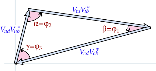
Figure 5: Graphical representation of the unitarity constraint $V_{ud}V_{ub}^{*}+V_{cd}V_{cb}^{*}+V_{td}V_{tb}^{*}=0$ as a triangle in the complex plane.

The rescaled unitarity triangle is derived from (103) by (a) choosing a phase convention such that $(V_{cd}V_{cb}^{*})$ is real, and (b) dividing the lengths of all sides by $|V_{cd}V_{cb}^{*}|$. Step (a) aligns one side of the triangle with the real axis, and step (b) makes the length of this side 1. The form of the triangle is unchanged. Two vertices of the rescaled unitarity triangle are thus fixed at (0,0) and (1,0). The coordinates of the remaining vertex correspond to the Wolfenstein parameters $(\rho,\eta)$. The area of the rescaled unitarity triangle is $|\eta|/2$.

Depicting the rescaled unitarity triangle in the $(\rho,\eta)$ plane, the lengths of the two complex sides are

$$R_{u}\equiv\left|{V_{ud}V_{ub}\over V_{cd}V_{cb}}\right|=\sqrt{\rho^{2}+\eta^{2}},\ \ \ R_{t}\equiv\left|{V_{td}V_{tb}\over V_{cd}V_{cb}}\right|=\sqrt{(1-\rho)^{2}+\eta^{2}}.$$ (104)

The three angles of the unitarity triangle are defined as follows [73, 74]:

$$\alpha\equiv\arg\left[-{V_{td}V_{tb}^{*}\over V_{ud}V_{ub}^{*}}\right],\ \ \ \beta\equiv\arg\left[-{V_{cd}V_{cb}^{*}\over V_{td}V_{tb}^{*}}\right],\ \ \ \gamma\equiv\arg\left[-{V_{ud}V_{ub}^{*}\over V_{cd}V_{cb}^{*}}\right].$$ (105)

They are physical quantities and can be independently measured by CP asymmetries in $B$ decays. It is also useful to define the two small angles of the unitarity triangles (102,101):

$$\beta_{s}\equiv\arg\left[-{V_{ts}V_{tb}^{*}\over V_{cs}V_{cb}^{*}}\right],\ \ \ \beta_{K}\equiv\arg\left[-{V_{cs}V_{cd}^{*}\over V_{us}V_{ud}^{*}}\right].$$ (106)

.10 CPV in $B$ decays to final CP eigenstates

We define decay amplitudes of $B$ (which could be charged or neutral) and its CP conjugate $\overline{B}$ to a multi-particle final state $f$ and its CP conjugate $\overline{f}$ as

$$A_{f}=\langle f|{\cal H}|B\rangle\quad,\quad\overline{A}_{f}=\langle f|{\cal H}|\overline{B}\rangle\quad,\quad A_{\overline{f}}=\langle\overline{f}|{\cal H}|B\rangle\quad,\quad\overline{A}_{\overline{f}}=\langle\overline{f}|{\cal H}|\overline{B}\rangle\;,$$ (107)

where ${\cal H}$ is the Hamiltonian governing weak interactions. The action of CP on these states introduces phases $\xi_{B}$ and $\xi_{f}$ according to

$$CP\ |B\rangle = e^{+i\xi_{B}}\,|\overline{B}\rangle\quad,\quad CP\ |f\rangle=e^{+i\xi_{f}}\,|\overline{f}\rangle\;,$$

$$CP\ |\overline{B}\rangle = e^{-i\xi_{B}}\,|B\rangle\quad,\quad CP\ |\overline{f}\rangle=e^{-i\xi_{f}}\,|f\rangle\ ,$$ (108)

so that $(CP\ )^{2}=1$. The phases $\xi_{B}$ and $\xi_{f}$ are arbitrary and unphysical because of the flavor symmetry of the strong interaction. If CP is conserved by the dynamics, $[CP\ ,{\cal H}]=0$, then $A_{f}$ and $\overline{A}_{\overline{f}}$ have the same magnitude and an arbitrary unphysical relative phase

$$\overline{A}_{\overline{f}}=e^{i(\xi_{f}-\xi_{B})}\,A_{f}\;.$$ (109)

A state that is initially a superposition of ${B^{0}}$ and $\overline{B}{}^{0}$, say

$$|\psi(0)\rangle=a(0)|{B^{0}}\rangle+b(0)|\overline{B}{}^{0}\rangle\;,$$ (110)

will evolve in time acquiring components that describe all possible decay final states $\{f_{1},f_{2},\ldots\}$, that is,

$$|\psi(t)\rangle=a(t)|{B^{0}}\rangle+b(t)|\overline{B}{}^{0}\rangle+c_{1}(t)|f_{1}\rangle+c_{2}(t)|f_{2}\rangle+\cdots\;.$$ (111)

If we are interested in computing only the values of $a(t)$ and $b(t)$ (and not the values of all $c_{i}(t)$), and if the times $t$ in which we are interested are much larger than the typical strong interaction scale, then we can use a much simplified formalism [75]. The simplified time evolution is determined by a $2\times 2$ effective Hamiltonian ${\cal H}$ that is not Hermitian, since otherwise the mesons would only oscillate and not decay. Any complex matrix, such as ${\cal H}$, can be written in terms of Hermitian matrices $M$ and $\Gamma$ as

$${\cal H}=M-\frac{i}{2}\,\Gamma\;.$$ (112)

$M$ and $\Gamma$ are associated with $({B^{0}},\overline{B}{}^{0})\leftrightarrow({B^{0}},\overline{B}{}^{0})$ transitions via off-shell (dispersive) and on-shell (absorptive) intermediate states, respectively. Diagonal elements of $M$ and $\Gamma$ are associated with the flavor-conserving transitions ${B^{0}}\to{B^{0}}$ and $\overline{B}{}^{0}\to\overline{B}{}^{0}$ while off-diagonal elements are associated with flavor-changing transitions ${B^{0}}\leftrightarrow\overline{B}{}^{0}$.

The eigenvectors of ${\cal H}$ have well defined masses and decay widths. We introduce complex parameters $p$ and $q$ to specify the components of the strong interaction eigenstates, ${B^{0}}$ and $\overline{B}{}^{0}$, in the light ($B_{L}$) and heavy ($B_{H}$) mass eigenstates:

$$|B_{L,H}\rangle=p|{B^{0}}\rangle\pm q|\overline{B}{}^{0}\rangle$$ (113)

with the normalization $|p|^{2}+|q|^{2}=1$. The special form of Eq. (113) is related to the fact that CPT imposes $M_{11}=M_{22}$ and $\Gamma_{11}=\Gamma_{22}$. Solving the eigenvalue problem gives

$$\left(\frac{q}{p}\right)^{2}=\frac{M_{12}^{\ast}-(i/2)\Gamma_{12}^{\ast}}{M_{12}-(i/2)\Gamma_{12}}\;.$$ (114)

If either CP or T is a symmetry of ${\cal H}$, then $M_{12}$ and $\Gamma_{12}$ are relatively real, leading to

$$\left(\frac{q}{p}\right)^{2}=e^{2i\xi_{B}}\quad\Rightarrow\quad\left|\frac{q}{p}\right|=1\;,$$ (115)

where $\xi_{B}$ is the arbitrary unphysical phase introduced in Eq. (.10).

The real and imaginary parts of the eigenvalues of ${\cal H}$ corresponding to $|B_{L,H}\rangle$ represent their masses and decay-widths, respectively. The mass difference $\Delta m_{B}$ and the width difference $\Delta\Gamma_{B}$ are defined as follows:

$$\Delta m_{B}\equiv M_{H}-M_{L},\ \ \ \Delta\Gamma_{B}\equiv\Gamma_{H}-\Gamma_{L}.$$ (116)

Note that here $\Delta m_{B}$ is positive by definition, while the sign of $\Delta\Gamma_{B}$ is to be experimentally determined. The average mass and width are given by

$$m_{B}\equiv{M_{H}+M_{L}\over 2},\ \ \ \Gamma_{B}\equiv{\Gamma_{H}+\Gamma_{L}\over 2}.$$ (117)

It is useful to define dimensionless ratios $x$ and $y$:

$$x\equiv{\Delta m_{B}\over\Gamma_{B}},\ \ \ y\equiv{\Delta\Gamma_{B}\over 2\Gamma_{B}}.$$ (118)

Solving the eigenvalue equation gives

$$(\Delta m_{B})^{2}-{1\over 4}(\Delta\Gamma_{B})^{2}=(4|M_{12}|^{2}-|\Gamma_{12}|^{2}),\ \ \ \ \Delta m_{B}\Delta\Gamma_{B}=4{\cal R}e(M_{12}\Gamma_{12}^{*}).$$ (119)

All CP-violating observables in $B$ and $\overline{B}$ decays to final states $f$ and $\overline{f}$ can be expressed in terms of phase-convention-independent combinations of $A_{f}$, $\overline{A}_{f}$, $A_{\overline{f}}$ and $\overline{A}_{\overline{f}}$, together with, for neutral-meson decays only, $q/p$. CP violation in charged-meson decays depends only on the combination $|\overline{A}_{\overline{f}}/A_{f}|$, while CP violation in neutral-meson decays is complicated by ${B^{0}}\leftrightarrow\overline{B}{}^{0}$ oscillations and depends, additionally, on $|q/p|$ and on $\lambda_{f}\equiv(q/p)(\overline{A}_{f}/A_{f})$.

For neutral $D$, $B$, and $B_{s}$ mesons, $\Delta\Gamma/\Gamma\ll 1$ and so both mass eigenstates must be considered in their evolution. We denote the state of an initially pure $|{B^{0}}\rangle$ or $|\overline{B}{}^{0}\rangle$ after an elapsed proper time $t$ as $|{B^{0}}_{\mathrm{phys}}(t)\rangle$ or $|\overline{B}{}^{0}_{\mathrm{phys}}(t)\rangle$, respectively. Using the effective Hamiltonian approximation, we obtain

$$|{B^{0}}_{\rm phys}(t)\rangle = g_{+}(t)\,|{B^{0}}\rangle-\frac{q}{p}\ g_{-}(t)|\overline{B}{}^{0}\rangle,$$

$$|\overline{B}{}^{0}_{\rm phys}(t)\rangle = g_{+}(t)\,|\overline{B}{}^{0}\rangle-\frac{p}{q}\ g_{-}(t)|{B^{0}}\rangle\;,$$ (120)

where

$$g_{\pm}(t)\equiv\frac{1}{2}\left(e^{-im_{H}t-\frac{1}{2}\Gamma_{H}t}\pm e^{-im_{L}t-\frac{1}{2}\Gamma_{L}t}\right).$$ (121)

One obtains the following time-dependent decay rates:

$$\frac{d\Gamma[{B^{0}}_{\rm phys}(t)\to f]/dt}{e^{-\Gamma t}{\cal N}_{f}} = \left(|A_{f}|^{2}+|(q/p)\overline{A}_{f}|^{2}\right)\cosh(y\Gamma t)+\left(|A_{f}|^{2}-|(q/p)\overline{A}_{f}|^{2}\right)\cos(x\Gamma t)$$ (122)

$$+ 2\,{\cal R}e((q/p)A_{f}^{\ast}\overline{A}_{f})\sinh(y\Gamma t)-2\,{\cal I}m((q/p)A_{f}^{\ast}\overline{A}_{f})\sin(x\Gamma t)\;,$$

$$\frac{d\Gamma[\overline{B}{}^{0}_{\rm phys}(t)\to f]/dt}{e^{-\Gamma t}{\cal N}_{f}} = \left(|(p/q)A_{f}|^{2}+|\overline{A}_{f}|^{2}\right)\cosh(y\Gamma t)-\left(|(p/q)A_{f}|^{2}-|\overline{A}_{f}|^{2}\right)\cos(x\Gamma t)$$ (123)

$$+ 2\,{\cal R}e((p/q)A_{f}\overline{A}^{\ast}_{f})\sinh(y\Gamma t)-2\,{\cal I}m((p/q)A_{f}\overline{A}^{\ast}_{f})\sin(x\Gamma t)\;,$$

where ${\cal N}_{f}$ is a common normalization factor. Decay rates to the CP-conjugate final state $\overline{f}$ are obtained analogously, with ${\cal N}_{f}={\cal N}_{\overline{f}}$ and the substitutions $A_{f}\to A_{\overline{f}}$ and $\overline{A}_{f}\to\overline{A}_{\overline{f}}$ in Eqs. (122,123). Terms proportional to $|A_{f}|^{2}$ or $|\overline{A}_{f}|^{2}$ are associated with decays that occur without any net $B\leftrightarrow\overline{B}$ oscillation, while terms proportional to $|(q/p)\overline{A}_{f}|^{2}$ or $|(p/q)A_{f}|^{2}$ are associated with decays following a net oscillation. The $\sinh(y\Gamma t)$ and $\sin(x\Gamma t)$ terms of Eqs. (122,123) are associated with the interference between these two cases. Note that, in multi-body decays, amplitudes are functions of phase-space variables. Interference may be present in some regions but not others, and is strongly influenced by resonant substructure.

One possible manifestation of CP-violating effects in meson decays [76] is in the interference between a decay without mixing, ${B^{0}}\to f$, and a decay with mixing, ${B^{0}}\to\overline{B}{}^{0}\to f$ (such an effect occurs only in decays to final states that are common to ${B^{0}}$ and $\overline{B}{}^{0}$, including all CP eigenstates). It is defined by

$${\cal I}m(\lambda_{f})\neq 0\;,$$ (124)

with

$$\lambda_{f}\equiv\frac{q}{p}\frac{\overline{A}_{f}}{A_{f}}\;.$$ (125)

This form of CP violation can be observed, for example, using the asymmetry of neutral meson decays into final CP eigenstates $f_{CP\ }$

$${\cal A}_{f_{CP\ }}(t)\equiv\frac{d\Gamma/dt[\overline{B}{}^{0}_{\rm phys}(t)\to f_{CP\ }]-d\Gamma/dt[{B^{0}}_{\rm phys}(t)\to f_{CP\ }]}{d\Gamma/dt[\overline{B}{}^{0}_{\rm phys}(t)\to f_{CP\ }]+d\Gamma/dt[{B^{0}}_{\rm phys}(t)\to f_{CP\ }]}\;.$$ (126)

For $\Delta\Gamma=0$ and $|q/p|=1$ (which is a good approximation for $B$ mesons), ${\cal A}_{f_{CP\ }}$ has a particularly simple form [77, 78, 79]:

$${\cal A}_{f}(t) = S_{f}\sin(\Delta mt)-C_{f}\cos(\Delta mt),$$

$$S_{f} \equiv \frac{2\,{\cal I}m(\lambda_{f})}{1+|\lambda_{f}|^{2}},\ \ \ C_{f}\equiv\frac{1-|\lambda_{f}|^{2}}{1+|\lambda_{f}|^{2}}\;,$$ (127)

Consider the $B\to f$ decay amplitude $A_{f}$, and the CP conjugate process, $\overline{B}\to\overline{f}$, with decay amplitude $\overline{A}_{\overline{f}}$. There are two types of phases that may appear in these decay amplitudes. Complex parameters in any Lagrangian term that contributes to the amplitude will appear in complex conjugate form in the CP-conjugate amplitude. Thus their phases appear in $A_{f}$ and $\overline{A}_{\overline{f}}$ with opposite signs. In the Standard Model, these phases occur only in the couplings of the $W^{\pm}$ bosons and hence are often called “weak phases”. The weak phase of any single term is convention dependent. However, the difference between the weak phases in two different terms in $A_{f}$ is convention independent. A second type of phase can appear in scattering or decay amplitudes even when the Lagrangian is real. Their origin is the possible contribution from intermediate on-shell states in the decay process. Since these phases are generated by CP-invariant interactions, they are the same in $A_{f}$ and $\overline{A}_{\overline{f}}$. Usually the dominant rescattering is due to strong interactions and hence the designation “strong phases” for the phase shifts so induced. Again, only the relative strong phases between different terms in the amplitude are physically meaningful.

The ‘weak’ and ‘strong’ phases discussed here appear in addition to the ‘spurious’ CP-transformation phases of Eq. (109). Those spurious phases are due to an arbitrary choice of phase convention, and do not originate from any dynamics or induce any CP violation. For simplicity, we set them to zero from here on.

It is useful to write each contribution $a_{i}$ to $A_{f}$ in three parts: its magnitude $|a_{i}|$, its weak phase $\phi_{i}$, and its strong phase $\delta_{i}$. If, for example, there are two such contributions, $A_{f}=a_{1}+a_{2}$, we have

$$A_{f} = |a_{1}|e^{i(\delta_{1}+\phi_{1})}+|a_{2}|e^{i(\delta_{2}+\phi_{2})},$$

$$\overline{A}_{\overline{f}} = |a_{1}|e^{i(\delta_{1}-\phi_{1})}+|a_{2}|e^{i(\delta_{2}-\phi_{2})}.$$ (128)

Similarly, for neutral meson decays, it is useful to write

$$M_{12}=|M_{12}|e^{i\phi_{M}}\quad,\quad\Gamma_{12}=|\Gamma_{12}|e^{i\phi_{\Gamma}}\;.$$ (129)

Each of the phases appearing in Eqs. (.10,129) is convention dependent, but combinations such as $\delta_{1}-\delta_{2}$, $\phi_{1}-\phi_{2}$, $\phi_{M}-\phi_{\Gamma}$ and $\phi_{M}+\phi_{1}-\overline{\phi}_{1}$ (where $\overline{\phi}_{1}$ is a weak phase contributing to $\overline{A}_{f}$) are physical.

In the approximations that only a single weak phase contributes to decay, $A_{f}=|a_{f}|e^{i(\delta_{f}+\phi_{f})}$, and that $|\Gamma_{12}/M_{12}|=0$, we obtain $|\lambda_{f}|=1$ and the CP asymmetries in decays to a final CP eigenstate $f$ [Eq. (126)] with eigenvalue $\eta_{f}=\pm 1$ are given by

$${\cal A}_{f_{CP\ }}(t)={\cal I}m(\lambda_{f})\;\sin(\Delta mt)\;\ \mathrm{with}\ \ {\cal I}m(\lambda_{f})=\eta_{f}\sin(\phi_{M}+2\phi_{f}).$$ (130)

Note that the phase so measured is purely a weak phase, and no hadronic parameters are involved in the extraction of its value from ${\cal I}m(\lambda_{f})$.

.11 Supersymmetric flavor violation

.11.1 Mass insertions

Supersymmetric models provide, in general, new sources of flavor violation. We here present the formalism of mass insertions. We do that for the charged sleptons, but the formalism is straightforwardly adapted for squarks.

The supersymmetric lepton flavor violation is most commonly analyzed in the basis in which the charged lepton mass matrix and the gaugino vertices are diagonal. In this basis, the slepton masses are not necessarily flavor-diagonal, and have the form

$$\widetilde{\ell}_{Mi}^{*}(M^{2}_{\widetilde{\ell}})^{MN}_{ij}\widetilde{\ell}_{Nj}=(\widetilde{\ell}_{Li}^{*}\ \widetilde{\ell}_{Rk}^{*})\left(\begin{array}[]{cc}M^{2}_{Lij}&A_{il}v_{d}\\ A_{jk}v_{d}&M^{2}_{Rkl}\end{array}\right)\left(\begin{array}[]{c}\widetilde{\ell}_{Lj}\\ \widetilde{\ell}_{Rl}\end{array}\right),$$ (131)

where $M,N=L,R$ label chirality, and $i,j,k,l=1,2,3$ are generational indices. $M^{2}_{L}$ and $M^{2}_{R}$ are the supersymmetry breaking slepton masses-squared. The $A$ parameters enter in the trilinear scalar couplings $A_{ij}\phi_{d}\widetilde{\ell}_{Li}\widetilde{\ell}_{Rj}^{*}$, where $\phi_{d}$ is the down-type Higgs boson, and $v_{d}=\langle\phi_{d}\rangle$. We neglect small flavor-conserving terms involving $\tan\beta=v_{u}/v_{d}$.

In this basis, charged LFV takes place through one or more slepton mass insertion. Each mass insertion brings with it a factor of

$$\delta^{MN}_{ij}\equiv(M^{2}_{\widetilde{\ell}})^{MN}_{ij}/\tilde{m}^{2},$$ (132)

where $\tilde{m}^{2}$ is the representative slepton mass scale. Physical processes therefore constrain

$$(\delta^{MN}_{ij})_{\rm eff}\sim{\rm max}\left[\delta^{MN}_{ij},\delta^{MP}_{ik}\delta^{PN}_{kj},\ldots,(i\leftrightarrow j)\right].$$ (133)

For example,

$$(\delta^{LR}_{12})_{\rm eff}\sim{\rm max}\left[A_{12}v_{d}/\tilde{m}^{2},M^{2}_{L1k}A_{k2}v_{d}/\tilde{m}^{4},A_{1k}v_{d}M^{2}_{Rk2}/\tilde{m}^{4},\ldots,(1\leftrightarrow 2)\right].$$ (134)

Note that contributions with two or more insertions may be less suppressed than those with only one.

It is useful to express the $\delta^{MN}_{ij}$ mass insertions in terms of parameters in the mass basis. We can write, for example,

$$\delta^{LL}_{ij}=\frac{1}{\tilde{m}^{2}}\sum_{\alpha}K^{L}_{i\alpha}K^{L*}_{j\alpha}\Delta\tilde{m}^{2}_{L\alpha}.$$ (135)

Here, we ignore $L-R$ mixing, so that $K^{L}_{i\alpha}$ is the mixing angle in the coupling of a neutralino to $\ell_{Li}-\widetilde{\ell}_{L\alpha}$ (with $\ell_{i}=e,\mu,\tau$ denoting charged lepton mass eigenstates and $\widetilde{\ell}_{\alpha}=\widetilde{\ell}_{1},\widetilde{\ell}_{2},\widetilde{\ell}_{3}$ denoting charged slepton mass eigenstates), and $\Delta\tilde{m}^{2}_{L\alpha}=m^{2}_{\widetilde{\ell}_{L\alpha}}-\tilde{m}^{2}$. Using the unitarity of the mixing matrix $K^{L}$, we can write

$$\tilde{m}^{2}\delta^{LL}_{ij}=\sum_{\alpha}K^{L}_{i\alpha}K^{L*}_{j\alpha}(\Delta\tilde{m}^{2}_{L\alpha}+\tilde{m}^{2})=(M^{2}_{\widetilde{\ell}})^{LL}_{ij},$$ (136)

thus reproducing the definition (132).

In many cases, a two generation effective framework is useful. To understand that, consider a case where (no summation over $i,j,k$)

$$|K^{L}_{ik}K^{L*}_{jk}| \ll |K^{L}_{ij}K^{L*}_{j}|,$$

$$|K^{L}_{ik}K^{L*}_{jk}\Delta m^{2}_{\widetilde{\ell}_{Lk}\widetilde{\ell}_{Li}}| \ll |K^{L}_{ij}K^{L*}_{j}\Delta m^{2}_{\widetilde{\ell}_{Lj}\widetilde{\ell}_{Li}}|,$$ (137)

where $\Delta m^{2}_{\widetilde{\ell}_{j}\widetilde{\ell}_{i}}=m^{2}_{\widetilde{\ell}_{Lj}}-m^{2}_{\widetilde{\ell}_{Li}}$. Then, the contribution of the intermediate $\widetilde{\ell}_{k}$ can be neglected and, furthermore, to a good approximation $K^{L}_{ii}K^{L*}_{ji}+K^{L}_{ij}K^{L*}_{jj}=0$. For these cases, we obtain

$$\delta^{LL}_{ij}=\frac{\Delta m^{2}_{\widetilde{\ell}_{Lj}\widetilde{\ell}_{Li}}}{\tilde{m}^{2}}K^{L}_{ij}K^{L*}_{jj}.$$ (138)

.11.2 Neutral meson mixing

We consider the squark-gluino box diagram contribution to $D^{0}-\overline{D}^{0}$ mixing amplitude that is proportional to $K_{2i}^{u}K^{u*}_{1i}K_{2j}^{u}K^{u*}_{1j}$, where $K^{u}$ is the mixing matrix of the gluino couplings to left-handed up quarks and their up squark partners. (In the language of the mass insertion approximation, we calculate here the contribution that is $\propto[(\delta^{u}_{LL})_{12}]^{2}$.) We work in the mass basis for both quarks and squarks.

The contribution is given by

$$M_{12}^{D}=-i\frac{4\pi^{2}}{27}\alpha_{s}^{2}m_{D}f_{D}^{2}B_{D}\eta_{\rm QCD}\sum_{i,j}(K_{2i}^{u}K_{1i}^{u*}K_{2j}^{u}K_{1j}^{u*})(11\tilde{I}_{4ij}+4\tilde{m}_{g}^{2}I_{4ij}).$$ (139)

where

$$\tilde{I}_{4ij} \equiv \int\frac{d^{4}p}{(2\pi)^{4}}\frac{p^{2}}{(p^{2}-\tilde{m}_{g}^{2})^{2}(p^{2}-\tilde{m}_{i}^{2})(p^{2}-\tilde{m}_{j}^{2})}$$ (140)

$$= \frac{i}{(4\pi)^{2}}\left[\frac{\tilde{m}_{g}^{2}}{(\tilde{m}_{i}^{2}-\tilde{m}_{g}^{2})(\tilde{m}_{j}^{2}-\tilde{m}_{g}^{2})}\right.$$

$$+\left.\frac{\tilde{m}_{i}^{4}}{(\tilde{m}_{i}^{2}-\tilde{m}_{j}^{2})(\tilde{m}_{i}^{2}-\tilde{m}_{g}^{2})^{2}}\ln\frac{\tilde{m}_{i}^{2}}{\tilde{m}_{g}^{2}}+\frac{\tilde{m}_{j}^{4}}{(\tilde{m}_{j}^{2}-\tilde{m}_{i}^{2})(\tilde{m}_{j}^{2}-\tilde{m}_{g}^{2})^{2}}\ln\frac{\tilde{m}_{j}^{2}}{\tilde{m}_{g}^{2}}\right],$$

$$I_{4ij} \equiv \int\frac{d^{4}p}{(2\pi)^{4}}\frac{1}{(p^{2}-\tilde{m}_{g}^{2})^{2}(p^{2}-\tilde{m}_{i}^{2})(p^{2}-\tilde{m}_{j}^{2})}$$ (141)

$$= \frac{i}{(4\pi)^{2}}\left[\frac{1}{(\tilde{m}_{i}^{2}-\tilde{m}_{g}^{2})(\tilde{m}_{j}^{2}-\tilde{m}_{g}^{2})}\right.$$

$$+\left.\frac{\tilde{m}_{i}^{2}}{(\tilde{m}_{i}^{2}-\tilde{m}_{j}^{2})(\tilde{m}_{i}^{2}-\tilde{m}_{g}^{2})^{2}}\ln\frac{\tilde{m}_{i}^{2}}{\tilde{m}_{g}^{2}}+\frac{\tilde{m}_{j}^{2}}{(\tilde{m}_{j}^{2}-\tilde{m}_{i}^{2})(\tilde{m}_{j}^{2}-\tilde{m}_{g}^{2})^{2}}\ln\frac{\tilde{m}_{j}^{2}}{\tilde{m}_{g}^{2}}\right].$$

We now follow the discussion in refs. [21, 80]. To see the consequences of the super-GIM mechanism, let us expand the expression for the box integral around some value $\tilde{m}^{2}_{q}$ for the squark masses-squared:

$$I_{4}(\tilde{m}_{g}^{2},\tilde{m}_{i}^{2},\tilde{m}_{j}^{2}) = I_{4}(\tilde{m}_{g}^{2},\tilde{m}_{q}^{2}+\delta\tilde{m}_{i}^{2},\tilde{m}_{q}^{2}+\delta\tilde{m}_{j}^{2})$$ (142)

$$= I_{4}(\tilde{m}_{g}^{2},\tilde{m}_{q}^{2},\tilde{m}_{q}^{2})+(\delta\tilde{m}_{i}^{2}+\delta\tilde{m}_{j}^{2})I_{5}(\tilde{m}_{g}^{2},\tilde{m}_{q}^{2},\tilde{m}_{q}^{2},\tilde{m}_{q}^{2})$$

$$+ \frac{1}{2}\left[(\delta\tilde{m}_{i}^{2})^{2}+(\delta\tilde{m}_{j}^{2})^{2}+2(\delta\tilde{m}_{i}^{2})(\delta\tilde{m}_{j}^{2})\right]I_{6}(\tilde{m}_{g}^{2},\tilde{m}_{q}^{2},\tilde{m}_{q}^{2},\tilde{m}_{q}^{2},\tilde{m}_{q}^{2})+\cdots,$$

where

$$I_{n}(\tilde{m}_{g}^{2},\tilde{m}_{q}^{2},\ldots,\tilde{m}_{q}^{2})\equiv\int\frac{d^{4}p}{(2\pi)^{4}}\frac{1}{(p^{2}-\tilde{m}_{g}^{2})^{2}(p^{2}-\tilde{m}_{q}^{2})^{n-2}},$$ (143)

and similarly for $\tilde{I}_{4ij}$. Note that $I_{n}\propto(\tilde{m}_{q}^{2})^{n-2}$ and $\tilde{I}_{n}\propto(\tilde{m}_{q}^{2})^{n-3}$. Thus, using $x\equiv\tilde{m}_{g}^{2}/\tilde{m}_{q}^{2}$, it is customary to define

$$I_{n}\equiv\frac{i}{(4\pi)^{2}(\tilde{m}_{q}^{2})^{n-2}}f_{n}(x),\ \ \ \ \tilde{I}_{n}\equiv\frac{i}{(4\pi)^{2}(\tilde{m}_{q}^{2})^{n-3}}\tilde{f}_{n}(x).$$ (144)

The unitarity of the mixing matrix implies that

$$\sum_{i}(K_{2i}^{u}K_{1i}^{u*}K_{2j}^{u}K_{1j}^{u*})=\sum_{j}(K_{2i}^{u}K_{1i}^{u*}K_{2j}^{u}K_{1j}^{u*})=0.$$ (145)

Consequently, the terms that are proportional $f_{4},\tilde{f}_{4},f_{5}$ and $\tilde{f}_{5}$ vanish in their contribution to $M_{12}$. When $\delta\tilde{m}_{i}^{2}\ll\tilde{m}_{q}^{2}$ for all $i$, the leading contributions to $M_{12}$ come from $f_{6}$ and $\tilde{f}_{6}$. We learn that for quasi-degenerate squarks, the leading contribution is quadratic in the small mass-squared difference. The functions $f_{6}(x)$ and $\tilde{f}_{6}(x)$ are given by

$$f_{6}(x) = \frac{6(1+3x)\ln x+x^{3}-9x^{2}-9x+17}{6(1-x)^{5}},$$

$$\tilde{f}_{6}(x) = \frac{6x(1+x)\ln x-x^{3}-9x^{2}+9x+1}{3(1-x)^{5}}.$$ (146)

For example, with $x=1$, $f_{6}(1)=-1/20$ and $\tilde{f}_{6}=+1/30$; with $x=2.33$, $f_{6}(2.33)=-0.015$ and $\tilde{f}_{6}=+0.013$.

To further simplify things, let us consider a two generation case. Then

$$M_{12}^{D} \propto 2(K_{21}^{u}K_{11}^{u*})^{2}(\delta\tilde{m}_{1}^{2})^{2}+2(K_{22}^{u}K_{12}^{u*})^{2}(\delta\tilde{m}_{2}^{2})^{2}+(K_{21}^{u}K_{11}^{u*}K_{22}^{u}K_{12}^{u*})(\delta\tilde{m}_{1}^{2}+\delta\tilde{m}_{2}^{2})^{2}$$ (147)

$$= (K^{u}_{21}K_{11}^{u*})^{2}(\tilde{m}_{2}^{2}-\tilde{m}_{1}^{2})^{2}.$$

We thus rewrite Eq. (139) for the case of quasi-degenerate squarks:

$$M_{12}^{D}=\frac{\alpha_{s}^{2}m_{D}f_{D}^{2}B_{D}\eta_{\rm QCD}}{108\tilde{m}_{q}^{2}}[11\tilde{f}_{6}(x)+4xf_{6}(x)]\frac{(\Delta\tilde{m}^{2}_{21})^{2}}{\tilde{m}_{q}^{4}}(K_{21}^{u}K_{11}^{u*})^{2}.$$ (148)

For example, for $x=1$, $11\tilde{f}_{6}(x)+4xf_{6}(x)=+0.17$. For $x=2.33$, $11\tilde{f}_{6}(x)+4xf_{6}(x)=+0.003$.

Bibliography

G.C. Branco, L. Lavoura and J.P. Silva, CP Violation (Oxford University Press, Oxford, 1999).
H.R. Quinn and Y. Nir, The Mystery of the Missing Antimatter (Princeton University Press, Princeton, 2007).

References

- [1] M. Kobayashi and T. Maskawa, Prog. Theor. Phys. 49 (1973) 652.
- [2] N. Cabibbo, Phys. Rev. Lett. 10 (1963) 531.
- [3] A. B. Carter and A. I. Sanda, Phys. Rev. Lett. 45 (1980) 952; Phys. Rev. D 23 (1981) 1567.
- [4] I. I. Y. Bigi and A. I. Sanda, Nucl. Phys. B 193 (1981) 85.
- [5] G. Buchalla, A. J. Buras, and M. E. Lautenbacher, Rev. Mod. Phys. 68 (1996) 1125 [arXiv:hep-ph/9512380].
- [6] Y. Grossman, A. L. Kagan and Z. Ligeti, Phys. Lett. B 538 (2002) 327 [arXiv:hep-ph/0204212].
- [7] H. Boos, T. Mannel and J. Reuter, Phys. Rev. D 70 (2004) 036006 [arXiv:hep-ph/0403085].
- [8] H. n. Li and S. Mishima, JHEP 0703 (2007) 009 [arXiv:hep-ph/0610120].
- [9] M. Gronau and J. L. Rosner, Phys. Lett. B 672 (2009) 349 [arXiv:0812.4796 [hep-ph]].
- [10] Y. Amhis et al. [Heavy Flavor Averaging Group Collaboration], arXiv:1207.1158 [hep-ex] and online update at http://www.slac.stanford.edu/xorg/hfag.
- [11] J. Beringer et al. [Particle Data Group Collaboration], Phys. Rev. D 86 (2012) 010001.
- [12] CKMfitter Group (J. Charles et al.), Eur. Phys. J. C41 (2005) 1 [hep-ph/0406184], updated results and plots available at: http://ckmfitter.in2p3.fr
- [13] Y. Nir, Nucl. Phys. Proc. Suppl. 117 (2003) 111 [arXiv:hep-ph/0208080].
- [14] Y. Grossman, Y. Nir and M. P. Worah, Phys. Lett. B 407 (1997) 307 (1997).
- [15] Y. Grossman, Y. Nir and G. Raz, Phys. Rev. Lett. 97 (2006) 151801 [arXiv:hep-ph/0605028].
- [16] M. Bona et al. [UTfit Collaboration], JHEP 0803 (2008) 049 [arXiv:0707.0636 [hep-ph]].
- [17] G. C. Branco, L. Lavoura and J. P. Silva, CP violation, Clarendon Press, Oxford (1999).
- [18] I. I. Y. Bigi and N. G. Uraltsev, Nucl. Phys. B 592 (2001) 92 [arXiv:hep-ph/0005089].
- [19] A. F. Falk, Y. Grossman, Z. Ligeti and A. A. Petrov, Phys. Rev. D 65 (2002) 054034 [arXiv:hep-ph/0110317].
- [20] A. F. Falk, Y. Grossman, Z. Ligeti, Y. Nir and A. A. Petrov, Phys. Rev. D 69 (2004) 114021 [arXiv:hep-ph/0402204].
- [21] G. Raz, Phys. Rev. D 66 (2002) 037701 [arXiv:hep-ph/0205310].
- [22] G. Isidori, Y. Nir and G. Perez, Ann. Rev. Nucl. Part. Sci. 60 (2010) 355 [arXiv:1002.0900 [hep-ph]].
- [23] N. Arkani-Hamed and S. Dimopoulos, JHEP 0506 (2005) 073 [arXiv:hep-th/0405159].
- [24] A. G. Cohen, D. B. Kaplan and A. E. Nelson, Phys. Lett. B 388 (1996) 588 [arXiv:hep-ph/9607394].
- [25] Y. Nir and N. Seiberg, Phys. Lett. B 309 (1993) 337 [arXiv:hep-ph/9304307].
- [26] M. Leurer, Y. Nir and N. Seiberg, Nucl. Phys. B 420 (1994) 468 [arXiv:hep-ph/9310320].
- [27] M. Ciuchini, E. Franco, D. Guadagnoli, V. Lubicz, M. Pierini, V. Porretti and L. Silvestrini, Phys. Lett. B 655 (2007) 162 [arXiv:hep-ph/0703204].
- [28] Y. Nir, JHEP 0705 (2007) 102 [arXiv:hep-ph/0703235].
- [29] O. Gedalia, J. F. Kamenik, Z. Ligeti and G. Perez, Phys. Lett. B 714 (2012) 55 [arXiv:1202.5038 [hep-ph]].
- [30] K. Blum, Y. Grossman, Y. Nir and G. Perez, Phys. Rev. Lett. 102 (2009) 211802 [arXiv:0903.2118 [hep-ph]].
- [31] G. D’Ambrosio, G. F. Giudice, G. Isidori and A. Strumia, Nucl. Phys. B 645 (2002) 155 [arXiv:hep-ph/0207036].
- [32] Y. Grossman, Y. Nir, J. Thaler, T. Volansky and J. Zupan, Phys. Rev. D 76 (2007) 096006 [arXiv:0706.1845 [hep-ph]].
- [33] V. Cirigliano, B. Grinstein, G. Isidori and M. B. Wise, Nucl. Phys. B 728 (2005) 121 [arXiv:hep-ph/0507001].
- [34] V. Cirigliano and B. Grinstein, Nucl. Phys. B 752 (2006) 18 [arXiv:hep-ph/0601111].
- [35] V. Cirigliano, G. Isidori and V. Porretti, Nucl. Phys. B 763 (2007) 228 [arXiv:hep-ph/0607068].
- [36] G. C. Branco, A. J. Buras, S. Jager, S. Uhlig and A. Weiler, JHEP 0709 (2007) 004 [arXiv:hep-ph/0609067].
- [37] M. C. Chen and H. B. Yu, Phys. Lett. B 672 (2009) 253 [arXiv:0804.2503 [hep-ph]].
- [38] E. Gross, D. Grossman, Y. Nir and O. Vitells, Phys. Rev. D 81 (2010) 055013 [arXiv:1001.2883 [hep-ph]].
- [39] J. L. Feng, C. G. Lester, Y. Nir and Y. Shadmi, Phys. Rev. D 77 (2008) 076002 [arXiv:0712.0674 [hep-ph]].
- [40] J. L. Feng, I. Galon, D. Sanford, Y. Shadmi and F. Yu, Phys. Rev. D 79 (2009) 116009 [arXiv:0904.1416 [hep-ph]].
- [41] J. L. Feng, S. T. French, C. G. Lester, Y. Nir and Y. Shadmi, Phys. Rev. D 80 (2009) 114004 [arXiv:0906.4215 [hep-ph]].
- [42] J. L. Feng et al., JHEP 1001 (2010) 047 [arXiv:0910.1618 [hep-ph]].
- [43] G. Hiller and Y. Nir, JHEP 0803 (2008) 046 [arXiv:0802.0916 [hep-ph]].
- [44] G. Hiller, Y. Hochberg and Y. Nir, JHEP 0903 (2009) 115 [arXiv:0812.0511 [hep-ph]].
- [45] G. Hiller, Y. Hochberg and Y. Nir, JHEP 1003 (2010) 079 [arXiv:1001.1513 [hep-ph]].
- [46] C. D. Froggatt and H. B. Nielsen, Nucl. Phys. B 147 (1979) 277.
- [47] M. Dine, R. G. Leigh and A. Kagan, Phys. Rev. D 48 (1993) 4269 [hep-ph/9304299].
- [48] A. E. Nelson and M. J. Strassler, JHEP 0009 (2000) 030 [arXiv:hep-ph/0006251];
- [49] N. Arkani-Hamed and M. Schmaltz, Phys. Rev. D 61 (2000) 033005 [hep-ph/9903417].
- [50] M. C. Gonzalez-Garcia, M. Maltoni, J. Salvado and T. Schwetz, JHEP 1212 (2012) 123 [arXiv:1209.3023 [hep-ph]].
- [51] L. J. Hall, H. Murayama and N. Weiner, Phys. Rev. Lett. 84 (2000) 2572 [hep-ph/9911341].
- [52] N. Haba and H. Murayama, Phys. Rev. D 63 (2001) 053010 [hep-ph/0009174].
- [53] A. de Gouvea and H. Murayama, Phys. Lett. B 573 (2003) 94 [hep-ph/0301050]; arXiv:1204.1249 [hep-ph].
- [54] S. Amitai, arXiv:1211.6252 [hep-ph].
- [55] P. F. Harrison, D. H. Perkins and W. G. Scott, Phys. Lett. B 530 (2002) 167 [hep-ph/0202074].
- [56] E. Ma and G. Rajasekaran, Phys. Rev. D 64 (2001) 113012 [hep-ph/0106291].
- [57] G. Altarelli and F. Feruglio, Rev. Mod. Phys. 82 (2010) 2701 [arXiv:1002.0211 [hep-ph]]. Nucl. Phys. B 741 (2006) 215 [hep-ph/0512103].
- [58] F. P. An et al. [DAYA-BAY Collaboration], Phys. Rev. Lett. 108 (2012) 171803 [arXiv:1203.1669 [hep-ex]].
- [59] S. Amitai, arXiv:1212.5165 [hep-ph].
- [60] G. Aad et al. [ATLAS Collaboration], Phys. Lett. B 716 (2012) 1 [arXiv:1207.7214 [hep-ex]].
- [61] S. Chatrchyan et al. [CMS Collaboration], Phys. Lett. B 716 (2012) 30 [arXiv:1207.7235 [hep-ex]].
- [62] D. Carmi, A. Falkowski, E. Kuflik and T. Volansky, arXiv:1206.4201 [hep-ph].
- [63] A. Dery, A. Efrati, Y. Hochberg and Y. Nir, JHEP 1305 (2013) 039 [arXiv:1302.3229 [hep-ph]].
- [64] A. Dery, A. Efrati, G. Hiller, Y. Hochberg and Y. Nir, arXiv:1304.6727 [hep-ph].
- [65] G. Blankenburg, J. Ellis and G. Isidori, Phys. Lett. B 712 (2012) 386 [arXiv:1202.5704 [hep-ph]].
- [66] R. Harnik, J. Kopp and J. Zupan, JHEP 1303 (2013) 026 [arXiv:1209.1397 [hep-ph]].
- [67] S. Davidson and P. Verdier, Phys. Rev. D 86 (2012) 111701 [arXiv:1211.1248 [hep-ph]].
- [68] A. Arhrib, Y. Cheng and O. C. W. Kong, Phys. Rev. D 87 (2013) 015025 [arXiv:1210.8241 [hep-ph]].
- [69] Y. Grossman and Y. Nir, Nucl. Phys. B 448 (1995) 30 [hep-ph/9502418].
- [70] L. Chau and W. Keung, Phys. Rev. Lett. 53 (1984) 1802.
- [71] L. Wolfenstein, Phys. Rev. Lett. 51 (1983) 1945.
- [72] A. J. Buras, M. E. Lautenbacher, and G. Ostermaier, Phys. Rev. D 50 (1994) 3433 [arXiv:hep-ph/9403384].
- [73] C. Dib, I. Dunietz, F. J. Gilman and Y. Nir, Phys. Rev. D 41 (1990) 1522.
- [74] J. L. Rosner, A. I. Sanda and M. P. Schmidt, EFI-88-12-CHICAGO [Presented at Workshop on High Sensitivity Beauty Physics, Batavia, IL, Nov 11-14, 1987].
- [75] V. Weisskopf and E. P. Wigner, Z. Phys. 63 (1930) 54; Z. Phys. 65 (1930) 18. [See Appendix A of P. K. Kabir, “The CP Puzzle: Strange Decays of the Neutral Kaon”, Academic Press (1968).]
- [76] Y. Nir, SLAC-PUB-5874 [Lectures given at 20th Annual SLAC Summer Institute on Particle Physics (Stanford, CA, 1992)].
- [77] I. Dunietz and J. L. Rosner, Phys. Rev. D 34 (1986) 1404.
- [78] Ya. I. Azimov, N. G. Uraltsev, and V. A. Khoze, Sov. J. Nucl. Phys. 45 (1987) 878 [Yad. Fiz. 45 (1987) 1412].
- [79] I. I. Bigi and A. I. Sanda, Nucl. Phys. B 281 (1987) 41.
- [80] Y. Nir and G. Raz, Phys. Rev. D 66 (2002) 035007 [arXiv:hep-ph/0206064].