Complex behaviour in cyclic competition bimatrix games
Department of Mathematics, Imperial College London
180 Queen’s Gate, SW7 2AZ London
Abstract. We consider an example of cyclic competition bimatrix game which is a Rock-Scissors-Paper game with assumption about perfect memory of the playing agents. At first we investigate the dynamics in the neighbourhood of the Nash equilibrium as well as the dynamics on the boundary of codimension 1 - that is when one of the strategies is not played by any agent. For the analysis of the asymptotic behaviour close to the boundary of state space, we provide the description of a naturally appearing heteroclinic network. Due to the symmetry, the heteroclinic network induces a quotient network. This quotient network is investigated as well. In the literature this model was already studied, but unfortunately the results stated there are invalid, as we will show in this paper. It turns out that certain types of behaviour are never possible or appear in the system only for some parameter values, contradicting what was stated before in the literature. Moreover, the parameter space is divided into four regions where we observe either irregular behaviour, or preference to follow an itinerary consisting of strategies for which one or the other agent does not lose, or they alternate in winning. These regions in parameter space are separated by two analytical curves and lines where the game is either symmetric (system is not linearisable at stationary saddle points) or is zero-sum and the system is Hamiltonian. On each of these curves we observe different bifurcation scenarios: e.g. transition from order to chaos, or from one kind of stability to another kind, or just loss of one dimension of the local stable manifold of the subcycle.
Introduction
In the last years there was a huge interest in bimatrix games, learning games, models with applications to population dynamics and economics. This paper will consider one such model, that is a Rock-Scissors-Paper game described by the replicator equations, which is a simplified model of a cyclic competition bimatrix game. This model was derived in e.g. [18]. Here we will mainly refer to four papers on this topic:
Aguiar M.A.D., Castro S.B.S.D ”Chaotic switching in a two-person game”, (Physica D 239 (2010) 1598-1609)
and three others by Sato et al. [18], [16], [17].
We suggest introductions of mentioned papers to the readers interested in the history of this particular problem and bimatrix games in general.
In the paper by Aguiar and Castro, the authors considered the same model as we do.
However, in their paroofs and their analysis, they made a ”simplifying assumption” namely that a certain transition maps between sections associated to stationary points in the heteroclinic network are ”identity maps” in the natural coordinates. As we will see in this paper this assumption is not valid in this model. It turns out that when uses the correct transition map, the results one obtains are rather different from those stated in Aguiar&Castro. A simple consideration based on the mean value theorem shows that it is impossible to assume that these transition maps are ”identity maps”.
In proposition 9, we compute the linear part of the transition maps in convenient local coordinates. This together with lemma 2, shows that the transition maps are in fact affine mappings. In proposition 12 we present the approximation of the composition of local maps with transition maps after rescaling of the coordinates, the final form of these compositions resemble expressions from Aguiar& Castro paper.
In theorem 4.5 of Aguiar&Castro, they claim that there is infinite switching near the heteroclinic network . However as we will show in this paper, this result is incorrect. The first reason for this is the following:
Theorem 3.
For every the finite itineraries of the form and are not attainable for - sufficiently small.
Moreover, in section 5 we will provide examples showing that attainability of some finite itineraries in arbitrarily small neighbourhood of the heteroclinic network strongly depends on the parameter values of the system.
Theorem 4.8, from Aguiar&Castro paper, states that for the cycle is relatively asymptotically stable (and cannot be essentially asymptotically stable), while for cycles are relatively asymptotically stable.
We correct this statements in the theorems 1 and 2:
Theorem 1.
For , the cycle is essentially asymptotically stable.
Theorem 2.
For some open regions in parameter space , cycles and , respectively, are neither almost completely unstable nor essentially asymptotically stable. For each of them, there exist open set of points in the phase space which is attracted to the respective cycle.
In the papers by Sato et al. [18], [16], [17], the derivation of the equations for the RSP game is presented. As well - these equations are transformed into other coordinates which are numerically stable, hence very useful for the numerical simulations. The authors gave partial and vague description of the global behaviour in the phase space, depending on the parameter values and based on the numerical investigations. However they mainly concentrate on the case . The numerical results reported in these papers are not compatible with each other and also with our results.
1.1 Organisation of the paper
We divide this paper into 7 sections.
In the second section we give the introduction to the model, characterize Nash equilibrium and we explain the global behaviour on the boundaries of codimensions and .
Following section provides full construction of the heteroclinic network naturally appearing in the system as well as all of the transition maps associated to this network.
Asymptotic analysis, stability of the cycles within the network and bifurcations happening in the system are described in section 4. We also present the link between our model and the one introduced by Aguiar&Castro, and correct some of their results.
Section number five, consists of examples showing some phenomenon in the system - attainability of the itineraries along heteroclinic orbits as a dependence of parameter values , . We present our examples contradicting the main results from AguiarCastro paper and start explaining our presumptions about the global behaviour in the system as well as local behaviour near the heteroclinic network.
In the sixth section we present our numerical investigations and compare it to Sato’s et al simulations [16], [17], [18]. We present our presumptions about the way the chaos might be born, we explain the obstacles that forbid us from proving our conjectures.
Finally, in the last section we make conclusions, discuss open questions and future work.
Preliminaries
We consider the Rock-Scissors-Paper game, played by two agents X and Y.
Let denote the probability that player X (resp. Y) plays Rock, Scissors or Paper. Obviously , . For each player, the state space is a two-dimensional simplex, hence the whole state space for played game is . The interaction matrices after normalization are given by:
| (2.1) | |||
with , the rewards for ties.
Assuming perfect memory of players, the dynamics are described by the replicator equations (see [18]):
| (2.2) |
with .
After substitutions , we will consider it as a differential equation:
| (2.3) |
with constraints , .
Let us denote the canonical basis in by .
Proposition 1.
The system (2.2) is invariant under action of the group generated by the cycle of order :
| (2.4) |
Equation (2.3) possesses following equilibria:
Proposition 2.
Nash equilibrium of the system
Proposition 3.
6 equilibria of (1,2,1) type (1-dim. stable manifold, 2-dim. center manifold, 1-dim. unstable manifold), which are centers within the 2 dimensional invariant subspaces.
Proposition 5.
9 equilibria of the form , where , which are all of (2,2) saddle type.
2.1 Nash equilibrium
Definition 1.
is a Nash equilibrium of the system iff and , for all .
In the bimatrix game in which there is only one Nash equilibrium, it can be found as the intersection of the nullclines (here of the equation (2.2)).
It is commonly known that system (2.2), is Hamiltonian for , that is when (see [9], [16]). Moreover it was proved that in this case all trajectories have on average the same payoff as the Nash equilibrium [18]. On the other hand, on any given step huge deviations from the payoff, when playing Nash equilibrium, can be observed. Thus, a risk averse agent would prefer the Nash equilibrium to a chaotic orbit. [16]
In the sixth section we will make use of the following proposition.
Proposition 2.
Nash equilibrium of the system , which is of saddle type for (or a center in the Hamiltonian case), with eigenvalues
where ,
Proof.
One can see that
in particular
and
which by the definition means that is a Nash equilibrium. Note that for and , we have , so it follows that . On the other hand , implies . Hence , . Moreover we see that:
. In such a case we have that . Consider then a Lyapunov function
From Jensen’s inequality , with equality if and only if . Moreover since and :
So either is a hyperbolic point of type or is a center. ∎
2.2 Dynamics on the boundaries of codimensions 2 and 1
If each of the players is restricted to only two strategies, then all orbits are periodic and spiral around one of the 6 equilibria or they converge to draw with time tending to . The latter case occurs for the system restricted to the subspaces , .
Proposition 3.
There are 6 equilibria of (1,2,1) type (1-dim. stable manifold, 2-dim. center manifold, 1-dim. unstable manifold), which are centers within the 2 dimensional invariant subspaces (where the system is integrable), and have one dimensional stable and unstable manifolds , :
Proof.
For one can compute the eigenvalues of linearized system to be
Eigenvectors corresponding to purely imaginary eigenvalues lie within subspace , . Restricting our system to this subspace (that is substituting and in the equation), we find the Lyapunov function for within subspace , :
One can see that for (moreover ) and
which proves that is a center within subspace , .
To prove that, for , stable manifold of is contained in the set , let us note that the system is Hamiltonian in so if some part of this stable manifold was included in then on the whole of unstable manifold the function , defined in the previous proposition, would be constant which is impossible since when .
In general, note that the eigenvector corresponding to the eigenvalue is equal to
Let us write
It is easy to see that for all we have . So for a point which belongs to the stable manifold of the point and is very close to , we may assume that
(the second case when , , can be treated in the same way). We want to prove that projection of the stable manifold on the -coordinate lies in the set , so it suffices to prove that with the above assumptions on and with we have (or if we change the signs of ). Obviously on the subset and
Since and is small enough then
If then obviously
since , otherwise we have
Since for any fixed the following inequality is satisfied , we can choose so small such that is close enough to and then , which proves that projection of stable manifold on the -coordinate lies in the set ∎
(a)
(b)
(c)
(d)
On the boundary of codimension 1, the trajectories of the game travel from one invariant hyperplane of dimension 2 to another one.
Proposition 4.
For all , the following inclusions hold:
Proof.
For and , note that with in the primary equation (2.2) we have:
if and if .
Moreover holds when either and or and .
Since and , this along with the above, means that the forward orbit of a point from will accumulate on the hyperplane and the backward orbit of a point from will accumulate on the hyperplane , where the motion is periodic.
∎
We believe that the following conjecture is worth further investigation.
Conjecture 1.
As one can check, there exist parameter values (e.g. , ) for which stable manifold of and unstable of seem to be very close.
This observation motivates the following question:
The set of pairs for which there is a heteroclinic orbit from to is isolated in the parameter space. The same question remains for the existence of other heteroclinic orbits, that is from:
to , to , to , to , to
Remark 1.
The existence of the heteroclinic orbit from to is equivalent to the existence of the zero of the function:
where are parameterizations (by s and t, respectively) of the manifolds and . This is a codimension 2 problem, hence in a family of two parameter vector fields one should expect the existence of the solution for the isolated set of parameters. (see [22], [27], [28], [29])
Heteroclinic network and its transition maps
Here we will show how heteroclinic network naturally appears in our system. We describe all of the maps associated with this network and process of deriving it. We will indicate the differences between our and Aguiar&Castro model. Although that one was incorrect, we have to take their observation into account:
Remark 2.
One can check that the system is linearizable for all except the case . The whole forthcoming analysis is conducted for .
Proposition 5.
The equation (2.3), possesses 9 equilibria of the form , where . They are all of (2,2) saddle type with eigenvalues (and corresponding eigenvectors) and stable/unstable manifolds since the system is invariant under the symmetry it suffices to provide the description for points , , :
Proof.
We find that the linearized system near is given by:
Hence, the searched eigenvalues are with the corresponding eigenvectors
.
is tangent at to the 2-dimensional subspace lin. Note that the subset is invariant, and moreover, when , , we have , . Furthermore the subset is invariant and there. So the whole set is attracted to points . From uniqueness of the existing stable manifold we have that . Analogically we prove
∎
Remark 3.
There are no other equilibria for (2.3) than described so far.
Let us denote .
Due to the above proposition, there exist a heteroclinic network consisting of these 9 equilibria and heteroclinic orbits written explicitly:
, , , , , ,
, , , , , ,
, , , , ,
Remark 4.
Heteroclinic orbits in this network are non-transversal intersections of stable and unstable manifolds of the appropriate equilibria.
Because of the above remark and hyperbolicity of the equilibria from the network, one does not necessarily expect chaotic switching infinitely close to the heteroclinic network as indeed we show. In fact we will discuss this matter more closely in sections 5 and 7.
Proposition 6.
The following matrices for are the transformation matrices from the eigenbasis at the point to the canonical basis of :
Proof.
consists of the eigenvectors of the linearized system at the point . ∎
Proposition 7.
At each of the points with from the heteroclinic network, the local coordinates of affine space in which this point is an origin, and the linearized system at this point is represented by the diagonal matrix (consisting of eigenvalues), are given by:
Proof.
Note that the transformation matrix from the eigenbasis (that is ) at the point to the canonical basis of is given by transformation matrix:
Moreover one can check that MacVU, hence the coordinates satisfying statements above should be given by condition: . This gives the thesis. ∎
Near each of the equilibrium from the heteroclinic network, we set four cross-sections to catch the orbits passing by close to this equilibrium. By introducing these cross-sections we can derive local maps near equilibriums and global maps from the neighbourhood of one equilibrium to another one along heteroclinic orbit, and in consequence discretize system in the neighbourhood of the heteroclinic network. Hence we can also check what kind of switching is possible and whether some particular trajectories infinitely close to the network are attainable.
Lemma 1.
The in/out sections near each of the points from the heteroclinic network, associated with the heteroclinic orbits between two points might be chosen as follows ( is arbitrarily small):
In local coordinates:
In local coordinates:
In local coordinates:
Proof.
Recall that in coordinates we have: and hence the heteroclinic orbit from to is parameterized by for . So in coordinates, we define the ”out” section from point towards point , to be the set for choosen arbitrarily small. Analogically, we define the ”in” section to the point from the point , to be the set ∎
In order to define global and local maps, we need to represent each of the ”in cross-sections” in two different coordinates. For the derivation of global maps we will use representation from proposition (1). The following proposition, enables us to compose local maps with global maps along cycles in the network.
Lemma 2.
Representations of the ”in” sections in the local coordinates of the points near which they are.
In local coordinates:
In local coordinates:
In local coordinates:
Proof.
Since the transformation from the coordinates to canonical ones is given by the mapping
and the transformation from canonical to is by
So the transformation from to coordinates is given by the mapping
Hence
∎
We find local maps, near each of the equilibrium from the heteroclinic network, in a standard way by linearizing the system near the equilibrium.
Proposition 8.
Local maps near each point of the heteroclinic network are given by the following formulas:
In coordinates:
- from to ,
- from to ,
In coordinates:
- from to ,
- from to ,
In coordinates:
- from to ,
- from to ,
Proof.
We approximate the system near by its linearization, in coordinates already:
The solution to it with initial condition is given by
For the point to belong to the out section , it is needed to have . Hence the local map to section is given by mapping
∎
In order to order to introduce global maps from ”out cross-sections” to ”in cross-sections”, we linearise the system along heteroclinic orbits. Note the difference between global maps from the proposition below and those from Aguiar&Castro paper. Although in section 4 we will find some similarities between the two approaches, we have to point out that we cannot just assume that the global maps are identity as this would lead to the contradiction with mean value theorem - in Aguiar&Castro paper no orbit from the neighbourhood of the heteroclinic orbit would ever leave it. The actual situation is obviously different, here the global maps derived below are in fact linear - given by the diagonal matrix with some of the entries bigger than 1.
Proposition 9.
Global maps along each heteroclinic orbit in the network are given by:
In coordinates:
In coordinates:
In coordinates:
Proof.
We compute global maps as shown below in the case of global map . In the initial equation (2.3), let us change the coordinates from the canonical basis to local coordinates in which is an origin, and . Let us rewrite the right-hand side of the system (after changing the coordinates) as
and the heteroclinic orbit from to by . Near one can write with -small. Then
Since (because of the invariance of ) and by the chain rule
we have that
| (3.1) |
Imposing initial condition ,
is the solution to the latter equation (3.1). The global map will be given by mapping
Hence in coordinates global map to has the form:
with fixed. ∎
Proposition 10.
The return map from any section within invariant square to itself is an identity map (but restricted to a smaller neighbourhood of origin in the cross section).
The same observation holds for the return maps within other invariant squares:
, , ,
,
Proof.
It suffices to show that the return map to the cross section within invariant square is an identity. For this, we compute
∎
Asymptotic dynamics near the network
In this section we will provide analytical proofs of numerical findings by Sato et al. [17] and proper analysis of the behaviour close to the heteroclinic network. In particular we will explain the differences and similarities between our model and the one built by Aguiar&Castro.
Recall that:
4.1 Dynamics near , , cycles
We start with an easy observation, that symmetry appearing in the system simplifies our computations along , , cycles, so instead of composing maps along six heteroclinic orbits, we can investigate part of it along two heteroclinic orbits.
Proposition 11.
The return maps to the sections , , through the , , cycles, respectively, are given by:
| (4.1) |
| (4.2) |
| (4.3) |
Proof.
For cycle, let
then
with , defined analogically (through cycle).
Due to the symmetry given by the action one can write:
∎
Let us identify, by symmetry , tie:=, win/loss:=, loss/win:=. Hence we can enumerate ”out cross-sections” as in the figure 4. Now, if is set to be a constant we can find approximations of the maps between the sections 1-6 in the limit of coordinates on the cross-sections tending to zero.
Proposition 12.
With and , it is possible to rescale coordinates linearly at the cross sections near: , , , so that the mappings are of the ”constant-free” form
Remark 5.
Note that in the proposition above, we have obtained the same formulas as Aguiar&Castro (upto some permutation, that comes from the difference between our and their transition maps), however the major difference is in the form of the domains of these maps (precisely: the constants appearing in the formulas), which in fact we will not use in the later analysis.
Definition 2.
A compact invariant set is called:
- asymptotically stable relative to if for every neighbourhood of there is a neighbourhood of such that for all we have and for all .
- completely unstable relative to if there is a neighbourhood of such that for all there is with .
Definition 3.
A compact invariant set is called essentially asymptotically stable if it is asymptotically stable relative to a set with the property that:
| (4.4) |
Definition 4.
A compact invariant set is almost completely unstable (a.c.u.) if it is completely unstable relative to a set with property (4.4).
Definition 5.
For , and small enough define
where and is the basin of attraction of , i.e. the set of points with .
Definition 6.
Local stability index at is defined to be:
where
We will make use of the following theorem (Theorem 3.5 in [12]), in order to prove, for some parameter values , essential asymptotic stability of and relative asymptotic stability of , .
Theorem 4.1.
(A.Lohse)
Let be a heteroclinic cycle or network with finitely many equilibria and connecting trajectories. Suppose that and that the local stability index exists and is not equal to zero for all . Then generically we have:
(i) is e.a.s. along all connecting trajectories
(i) is a.c.u. along all connecting trajectories
We prove here corrected statement of the first part of the Theorem 4.8 from Aguiar&Castro paper:
Theorem 1.
For , the cycle is essentially asymptotically stable.
Proof.
To prove that is e.a.s., one has to show that all of the local indices along the cycle are positive. From propositions 11 and 12, in the limit with and , the formulas for the maps along cycle simplify to the formulas from the paper by Aguiar&Castro. Although the domains of these maps are different by constants from the domains of maps in Aguilar&Castro paper, however for the computation of indices the only thing that counts, in this example, is the relationship between the exponents of coordinates in the maps and their domains as well - and this remains the same while taking and passing to the limit .
Furthermore, note that in the presence of symmetry in the system and formula (4.3), it suffices to compute only 2 indices for the map
instead of 6 indices for the return map .
Liliana Garrido Silva [8] was first that has computed these local indices for the Aguiar&Castro model and they are all positive for . Hence from the above reasoning, and by theorem (4.1), is an e.a.s cycle.
∎
Because of the Proposition 12, we can introduce logarithmic coordinates, useful for description of stability of the cycles and bifurcations happening in the system with varying.
Proposition 13.
The map from to through (and after identifying with by symmetry ) :
in logarithmic coordinates , has the form:
where
The eigenvalues and corresponding eigenvectors , , of matrix satisfy the following conditions:
- , while are complex conjugated and , , ,
-
-
- , ,
- , ,
- for :
- for :
Proposition 14.
The map from to through (and after identifying with by symmetry ):
in logarithmic coordinates , is given by:
where
The eigenvalues and corresponding eigenvectors , , of matrix satisfy the following conditions:
-
-
-
- for :
- for :
- for :
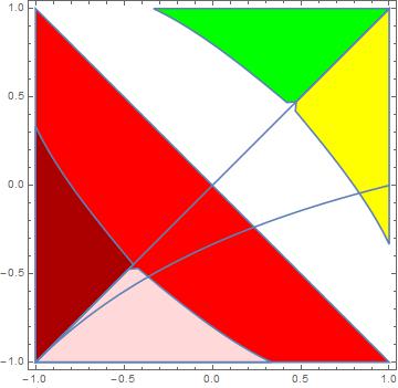
- in the yellow region
- in the white region where
- in the red region where
- in the light red region where
Remark 6.
We obtain the same proposition, as Prop. 14, for cycle by swapping with .
We are ready to prove that and are asymptotically stable relatively to some open set, however they cannot be essentially asymptotically stable according to the Theorem 4.1.
Theorem 2.
For some open regions (green), (yellow) in parameter space , cycles and , respectively, are neither almost completely unstable nor essentially asymptotically stable. For each of them, there exist an open set of points in the phase space which is attracted to the respective cycle.
Proof.
By propositions 11 and 14, the return map to the cross section through the whole cycle is given by
Let
where ( - eigenvectors from proposition 14). It suffices to show that for every from the yellow region, every compact interval and , there exist , big enough, such that for every , we have convergence to on all of the coordinates of the vectors and (as well for their coordinates have to be big enough). Now
and in logarithmic coordinates
Since for from the yellow region the following inequalities hold:
and
then while passing to the limit with , the leading terms are those multiplied by .
Hence, cycle is not almost completely unstable, however it cannot be essentially asymptotically stable since the domain of every second local map associated to cycle is a thin cusp, which means that the signs of the local indices alternate through the cycle.
∎
Remark 7.
In the same way we can prove about cycle weaker statement than the one from theorem 1.
4.2 Stability analysis of the cycles
In this subsection, we describe bifurcations happening in the sytem with varying. In the coordinates , and , let us denote
and the projection onto H, that is
wherever defined.
Following propositions are just consequences of the prop. 13, 14 and proof of the proposition 2.
Proposition 15.
Projection dynamics on of the cycle :
- 1.
-
2.
-for in the white region and , with :
-moreover for , with :
and every :
-if and , then there exist such that:
-
3.
-for from the red region and :
-for from the light red region and :
Proposition 16.
Projection dynamics on of the cycle :
-
1.
-for :
-
2.
-for and :
From the above propositions we can conclude that:
Proposition 17.
-
1.
for in the yellow region: and
-
2.
for in the white region: and
-
3.
for in the red region: and
-
4.
for in the light red region: and
Note that for there are no stable/unstable manifolds of , since .
Remark 8.
Analogical conclusions follow for cycle after swapping with .
We end this subsection with a concluding remark.
Remark 9.
With parameters passing from the red region to white region and finally to the yellow region, respectively - we observe a transition from essential asymptotic stability of through the case of Hamiltonian dynamics to the total disappearance of attraction properties and appearance of the 3-dimensional set attracted by cycle,
then appearance of 4-dimensional set attracted by cycle.
When crossing the line within white region or from the yellow to green region we observe that the set being attracted to cycle disappear and a new one attracted by cycle is born.
Shadowing between the ties, lack of infinite switching
As in the paper by Aguiar&Castro one can easily prove that there is switching along the heteroclinic orbits in the heteroclinic network. However in this section we point out that their result about infinite switching is incorrect. We provide some examples demonstrating that even attainability of some finite itineraries being infinitely close to the heteroclinic network depends strongly on parameter values .
Following Aguiar&Castro, we introduce the notion of finite switching:
Definition 7.
We say that there is switching along the heteroclinic orbit - from equilbrium to equilbrium , if for all equilbrias, say ,…,, for which there is a heteroclinic orbit from to ,…,, and all equilibria from which there is a heteroclinic orbit to , there exist a point such that:
for all and .
Definition 8.
If the process of switching along the heteroclinic orbit can be iterated infinitely many times then we say that there is infinite switching near the heteroclinic network.
Remark 10.
In generic case of heteroclinic network where heteroclinic orbits are non-transversal intersections of stable/unstable manifolds, one does not necessarily expect infinite switching to happen arbitrarily close to the heteroclinic network. We refer here to the work by Simon, Delshams and Zgliczyński [7], where they describe possible scenarios of switching along heteroclinic orbits in the non-transversal case and give explanation what one should expect at most from switching and about length of the itinerary, depending e.g. on the dimension of the phase space.
Proposition 18.
Finite itineraries following consecutively arbitrarily small neighbourhoods of the points:
and
are attainable for all
The next proposition presents a counterexample to the Theorem 4.5 about infinite switching claimed in Aguiar&Castro paper.
Theorem 3.
For every the finite itineraries of the form and are not attainable for - sufficiently small.
Proof.
For an itinerary take a point
Hence , . The necessary condition for the point
to lie in the domain of is the following inequality:
which is equivalent to
Note that
and
To see that this inequality cannot be satisfied it suffices to say that
for -small enough. ∎
Proposition 19.
For every , the finite itinerary
is not attainable for sufficiently small .
Proof.
For
we have , , . If
then the necessary condition for existence of this connection is , which is equivalent to
All of the powers of on the RHS are positive for , and for these parameters belong to some compact interval in . Hence RHS attains maximum for , and and is equal to
The power is bigger than for , and hence for small enough, the RHS is always smaller than LHS which is bounded from . ∎
In the same way we investigate the attainability of connections between ties, that is itineraries of the form:
(part of cycle)
We would like to end this subsection with small remark about the changes of probability that players will follow some finite itinerary depending on its length.
Proposition 20.
For arbitrarily fixed , there exists positive number , such that for the finite itinerary of the type ”” or ”, the measure of the set of points that follow from ’out cross-section’ near to ”in cross-section” before , through ”in cross-section” before , is less than times the measure of the set of points that follow from ’out cross-section’ near to ”out cross-section” after in the direction to . On the other hand measure of the points that follow itinerary of the length 4 is in the limit with approximately the same as the measure of points that follow the same itinerary extended by one equilibrium, in the order ”” or ”.
5.1 Chaotic switching
In Aguiar&Castro, the main theorem about RSP game was an incorrect statement about existence of infinite switching for all of the parameter values . We have already proven that it is not true, however there is still an open question about the existence of chaos in the system and switching which might be in fact described by subshift of finite type on two symbols (up to topological conjugation, e.g. see [21]).
We have already mentioned results by Delshams, Simon and Zgliczyński [7], which convince us that there has to exist some phenomenon in the system which forces existence of chaotic switching. In the sixth section we will provide numerical investigation in order to support our presumptions and intuition about what stays behind the irregular behaviour in the system (2.2).
Typically, examples of infinite switching that appear in the literature are associated to the existence of suspended horseshoes in the neighbourhood of the network (see e.g. [15]), in particular if there is an equilibrium in the network with complex eigenvalues - this can lead to the situation similar as in Shilnikov homoclinic bifurcation i.e. spiraling chaos. Although it is worth noting that A.Rodrigues [14] has given an example of an attracting homoclinic network exhibiting sensitive dependence on initial conditions, where the existence of infinite switching is not associated with suspended horseshoes. However there is a reason why we believe that there exist chaotic switching topologically conjugated to a subshift of finite type for all parameter values from the white region:
5.2 Finite switching
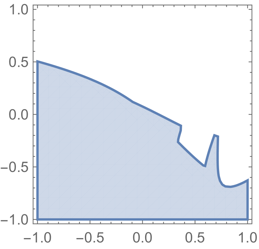
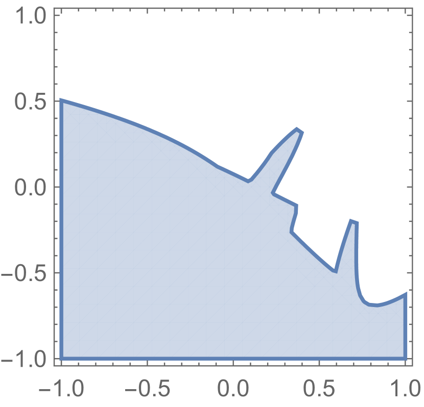
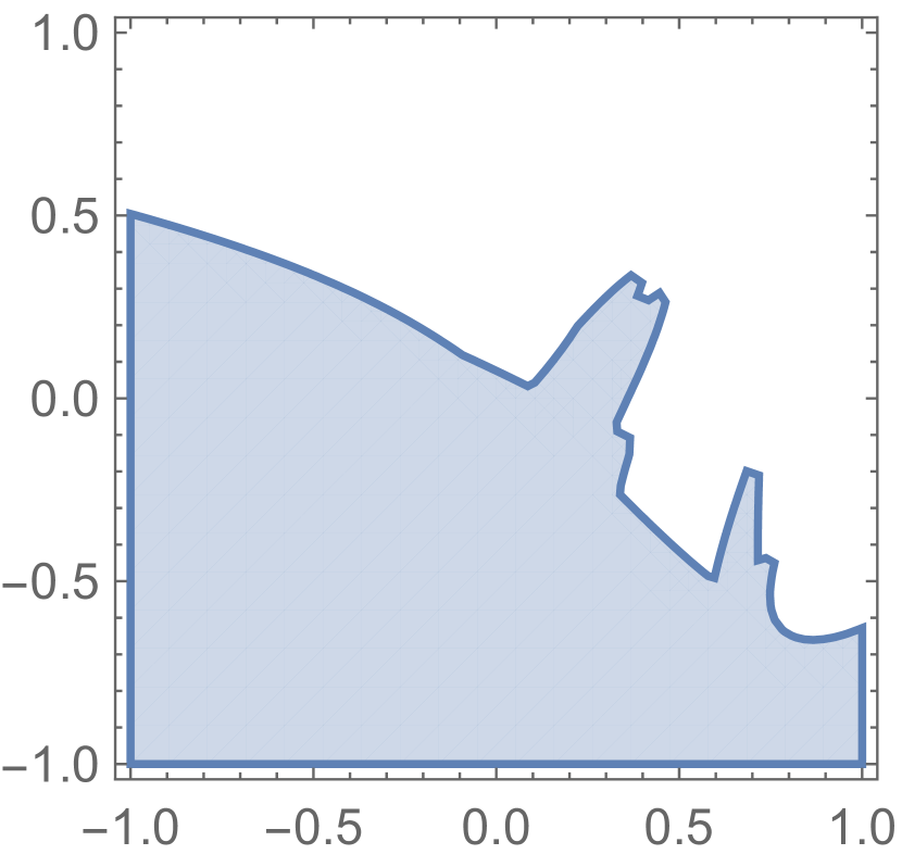
One can hope that it would be possible to determine exactly the form of eventual subshift of finite type describing switching near the system for all parameter values from the white region. In fact, it appears that it is hard to say precisely, for given parameter values , which finite itineraries are forbidden for orbits staying arbitrarily close to the network. Below we present some examples of finite itineraries about which we can say only when for sure they are not attainable.
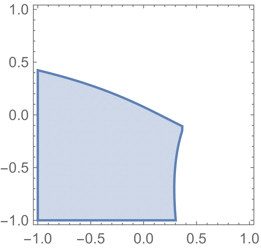
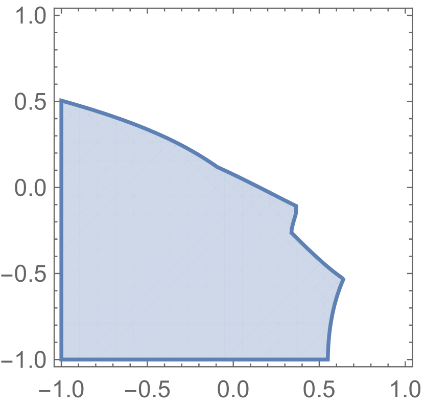
Shaded regions in the parameter space indicate parameter values for which the finite itinerary (written under the picture) consisting of numbered cross-sections in the quotient space (see figure 4),
are not attainable. For simplicity, we denote sequence (3, 4) as and (2,1) as .
![[Uncaptioned image]](/html/1605.00431/assets/x5.png)
(a) 3, 4, 3, 2, 1
![[Uncaptioned image]](/html/1605.00431/assets/x6.png)
(b) 3, 4, 3, 2, 1, 2, 1
![[Uncaptioned image]](/html/1605.00431/assets/x7.png)
(c) 3, 4, 3, 2, 1, 2, 1, 4, 3, 4, 3
![[Uncaptioned image]](/html/1605.00431/assets/x8.png)
(d) 3, 4, 3, 2, 1, 2, 1, 4, 3, 4, 3, 2, 1
![[Uncaptioned image]](/html/1605.00431/assets/x9.png)
(e) 3, 4, 3, 2, 1, 2, 1, 4, 3, 4, 3, 2, 1, 2, 1
![[Uncaptioned image]](/html/1605.00431/assets/x10.png)
(f) 3, 4, 3, 2, 1, 2, 1, 4, 3, 4, 3, 2, 1, 2, 1, 2, 1
(a) ,
(b) , , 3,
(c) , , , 3,
(d) , , , , , 3,
(e) , , , , , , 3, , , 4, , 3
(f) , , , , , , 3, , , 4, , 3,
(f) , , , , , , 3, , , 4, , 3, , ,
Numerical investigation
6.1 Sato’s et al. simulations
In this subsection we remind some of the numerical observations done by Y. Sato et al. (see [16], [17], [18]) and in the following subsection we compare it to our findings.
-
1.
With only quasiperiodic tori is observed. For some initial conditions, tori are knotted and form a trefoil.
-
2.
With Hamiltonian chaos can occur with positive-negative pairs of Lyapunov exponents. The dynamics is very rich in the sense that there are infinitely many distinct behaviors near the Nash equilibrium and a periodic orbit arbitrarily close to any chaotic one. (see [6])
-
3.
When the game is not zero-sum (), transients to heteroclinic cycles are observed. On the one hand, there are intermittent behaviors in which the time spent near pure strategies increases subexponentially with and on the other hand, with , chaotic transients persist.
-
4.
When , the behavior is intermittent and orbits are guided by the flow on edges of , which describes a network of possible heteroclinic cycles. Since action ties are not rewarded there is only one such cycle - . During the cycle each agent switches between almost deterministic actions in the order . The agents are out of phase with respect to each other and they alternate winning each turn.
-
5.
When , however, the orbit is an infinitely persistent chaotic transient. Since, in this case, agent can choose a tie, the cycles are not closed. For example, with , at , agent has the option of moving to instead of with a positive probability. This embeds an instability along the heteroclinic cycle and so orbits are chaotic.
-
6.
In [17], Lyapunov spectra, for different parameter values satisfying and different initial conditions, were investigated. In conclusion, as an evidence for Hamiltonian chaos for was presented the Lyapunov spectrum with the biggest Lyapunov exponent of order , and corresponding the second and third were of order .
6.2 Our numerical observations
Let us change the coordinates to the ones introduced in [18] (eq. (9)), which are useful since being more numerically stable. If , we substitute:
| (6.1) |
for . Then the equation (2.2) reduces to:
| (6.2) |
The reverse transformation is given by:
Sato’s et al. observations were based on simulations done by drawing points randomly from the phase space and integrating their orbits using either low order Runge-Kutta method or some symplectic integrator. However, there are known examples of systems for which usage of symplectic integrators leads to totally different simulations than those obtained by Taylor methods. The following example (Euler’s eq. 1760’) was provided by Prof. D.Wilczak:
One can compare simulated trajectory for the initial point , and see the differences between simulations using Taylor 30th order method and the symplectic Euler method. One of the reasons for the different portraits is the main disadvantage of the symplectic methods, that is the rounding of errors. For our purposes, we needed to utilise the integrator implemented in CAPD library [4], based on the Taylor method (order of the method can be choosen by the user, we have run the simulations with order from 10 to 30), with the time step fixed or adjusted after each iteration, in order to minimise the error.
6.3 Spectra of Lyapunov exponents
In order to determine the Lyapunov exponents , we utilised the algorithm of Ruelle and Eckmann based on the QR-decomposition method. As the Lyapunov exponents change slightly (difference for the consecutive time steps is of order ) for the integration time longer than , we decided to estimate them at time .
-
1.
For the Hamiltonian case, i.e. , we observe that the biggest Lyapunov exponent is of order . As expected for Hamiltonian systems are small (of order ) comparing to . These results are not compatible with Sato’s et al. numerics as we could not find for any point with the biggest Lyapunov exponent of order . In our simulations it was of order , in most cases, for the integration time from until . However, for these times, the conditions , were not satisfied even with the precision .
-
2.
For parameter values from the red and light red region we can observe two different patterns exhibited by the system for various initial conditions:
- either are of order and is of order or , small comparing to . For the initial point and parameter values , the Lyapunov spectrum is .
- or , are of order and are of order , , respectively (small comparing to . For the initial point and parameter values , the Lyapunov spectrum is . Two of the Lyapunov exponents being equal to zero, might indicate that some quantity is preserved by the system. -
3.
For parameter values from the white and yellow regions we can observe three patterns exhibited by the system for various initial conditions. Two of them are identical with those described above, another one is significantly different:
- , are of order , of order and of order or , which is small comparing to . In the white region, for the initial point and parameter values , the Lyapunov spectrum is . In the yellow region, for the initial point and parameter values , the Lyapunov spectrum is .
In each case, we observe that , so the system is dissipative, for all of the parameter values .
Remark 11.
At this place we want to thank Yuzuru Sato for his suggestion, that for the parameters from the white region, the biggest Lyapunov exponent is positive and the system (2.2) numerically appears to be chaotic.
6.4 Invariant manifolds of the Nash equilibrium
Remark 12.
Note that transformation of the form of the system (2.2), reverses the time and ordering of the cycles , and . As well it swaps and cycles. Due to this fact, it suffices to conduct forthcoming analysis only for the parameter values from the yellow region and white region below the diagonal (i.e. ).
Let us denote - normalised eigenvectors corresponding to the eigenvalues , from proposition (2), for the Nash equilibrium of the system (2.3). For , vectors having real coefficients:
| (6.3) |
span the tangent spaces to stable and unstable manifolds, i.e. and respectively.
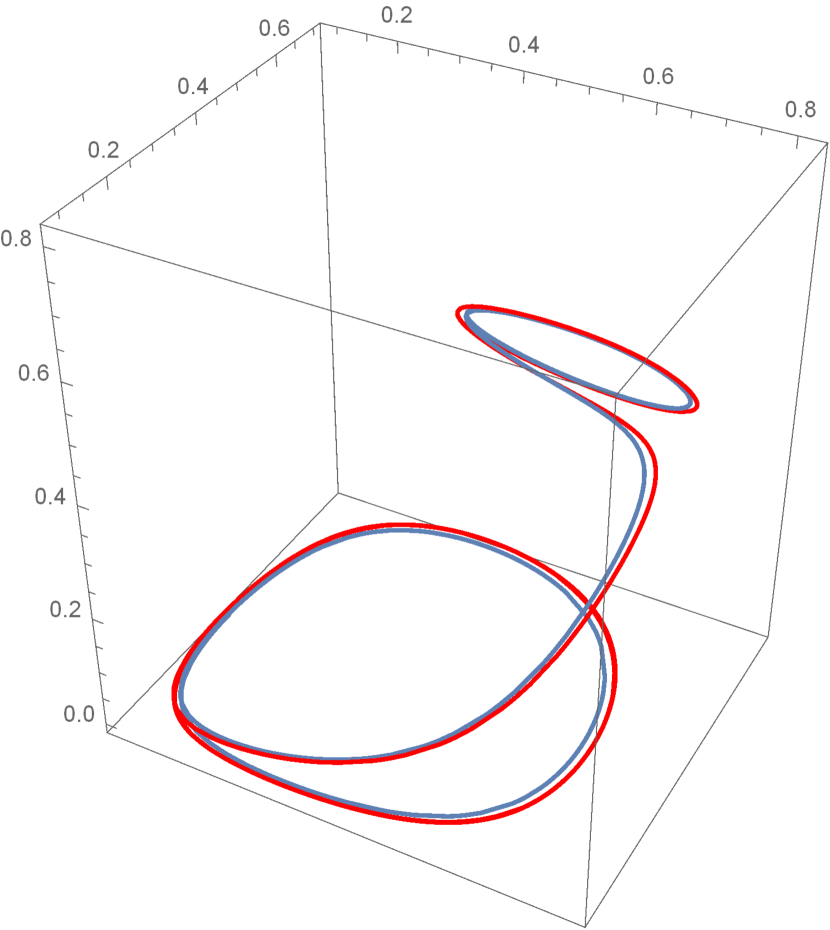
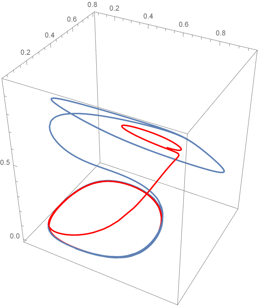
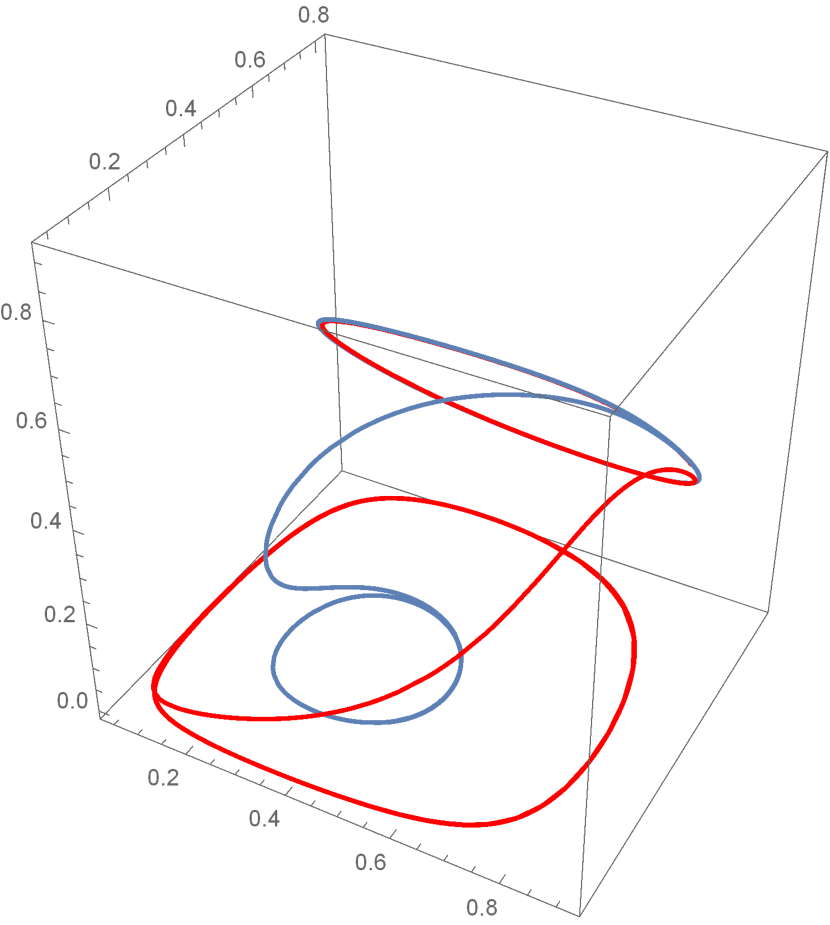
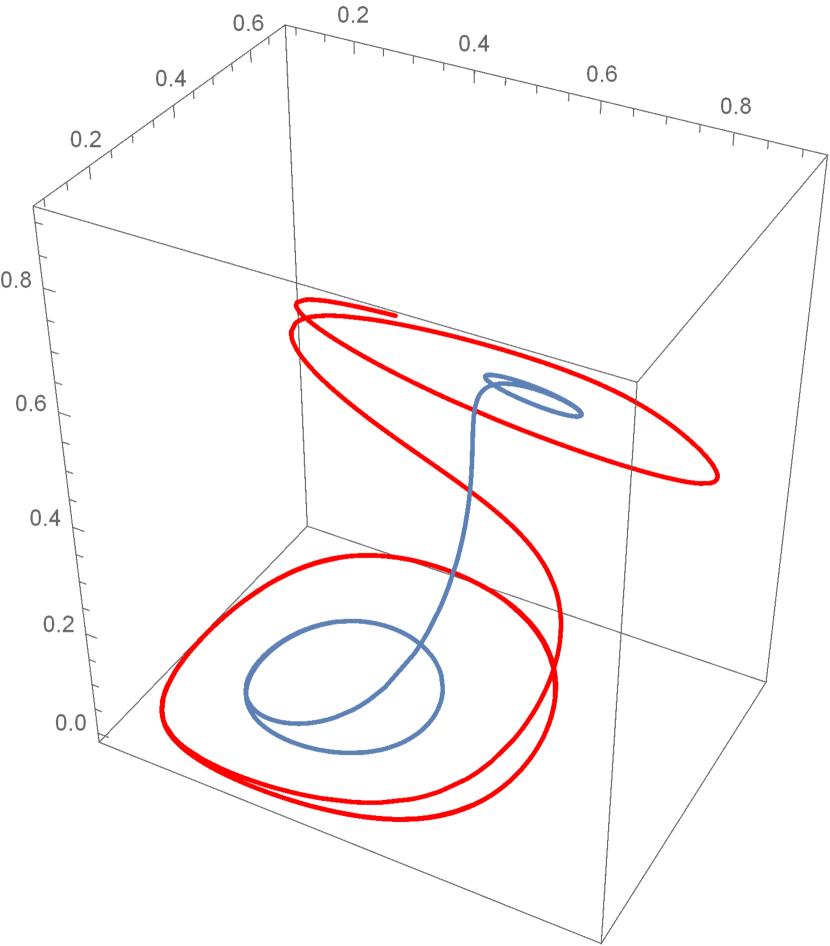
For the numeric simulations, in order to observe some irregular behaviour or convergence of orbits either to the cycles , , or , we set Poincare sections , and we:
- iterate backward the points from the stable tangent eigenspace (in coordinates) with , via the Poincare map associated to the sections ,
- iterate forward the points from the unstable tangent eigenspace (in coordinates) with , via the Poincare map associated to the sections ,
Observations on forward integration of points :
-
1.
for , from the white region,
- if , we observe irregular behaviour, we have not observed any symptoms of convergence within the first 200 iterations of the Poincare map
- if is small but not , the motion is irregular, however we can also observe iterations of to follow cycle for some time or for very few iterations come closer to cycle, but then come back to the irregularity
- for away from , we can observe either irregular behaviour for the whole simulation or it might happen that there are some irregularities at the beginning of iteration process, but the long term behaviour is the convergence to the cycle, this case requires additional investigation as we believe, the behaviour can depend on the sign of as well
- for being close to the boundary with yellow region, we observe fast convergence to the cycle -
2.
for , from the yellow region,
- we do not observe any symptoms of irregular behaviour of the iterations of points , almost all of them converge fastly to the cycle
Observations on backward integration of points are obviously similar in few aspects:
-
1.
for , from the white region,
- if , we observe irregular behaviour, we have not observed any symptoms of convergence of the iterations
- for away from , we can observe either irregular behaviour or it might happen that there are some irregularities (especially at the very beginning of iteration process), but the long term behaviour is the convergence to the cycle, this case as well requires additional investigation -
2.
for , from the yellow region,
- we do not observe any symptoms of irregular behaviour of the iterations of points , almost all of them converge fastly to the cycle
We do not precise what do we mean by ”fast convergence”, or far away from , as this is beyond our goals and scope of this paper. The purpose of conducting these numerical simulations was to explain: what kind of phenomenon can cause chaotic behaviour in the system or even near the heteroclinic network (switching possibly)? After introduction to this question in the subsection (5.1), we can now pose our questions and conjectures.
Conclusions and open questions
For from the yellow (resp. red) region away from antidiagonal almost all of the points from the stable (unstable) manifold after backward (forward) iteration by the Poincare map converge fastly to the cycles or what would suggest that there are not only heteroclinic connections Nash equilibrium – cycles, but that the intersections of stable (unstable) manifolds of the cycles with unstable (stable) manifolds of the Nash equilibrium are -dimensional. Do these intersections persist (presumably losing 1 dimension) when parameter values vary, especially when they are in white region?
Although essential asymptotic stability of cycle for does not exclude possibility of irregular behaviour in the system, it means however that closely to the equilibria , there is not much free space for switching from to the other cycles. Hence it seems reasonable, why Sato et al. did not observe numerically irregular behaviour, but mentioned in their papers only orbits guided by cycle.
The situation is different, however, for the cycle and parameter values in yellow region, since basins of attraction at every second equilibrium in this cycle are thin cusps, hence there is a lot of space to switch between the cycles. This, together with the fact that stable manifold of the cycle is -dimensional for , in the white region, would explain why Sato et al. concluded that for observed orbits are chaotic and the cycles are not closed, even for the , in the yellow region.
We have to point out that propositions 13, 14, guarantee locally strong contraction of the attracted open sets of points towards cycles and , for being very small or very big, respectively. Hence it seems plausible that the iterations of points from the tangent eigenspaces of the Nash equilibrium are converging fastly to the cycles - where we would look for the forward and backward heteroclinics from the Nash equilibrium. On the other hand, for close to , this local contraction is weak (for the cycle - of the 3-dimensional set of points), so our numerical observations about lack of convergence of points and towards the cycles, do not stay in the contradiction with e.g. essential asymptotic stability of the cycle. Irregular behaviour which we observe for these parameter values might come from the fact that the system then is close to the Hamiltonian one (the case ), where we observe (and it was broadly described in [16], [17], [18], [6]) Hamiltonian chaos.
The irregular behaviour we observe for , from the white region and the possible switching we expect to happen, might be as well a consequence of existence of homoclinic orbit to the cycles and (superhomoclinic orbit [20]), which might not pass very close to the Nash equilibrium, so we did not have the chance to notice it.
On the other hand, our numerical experiments suggest, that for some parameter values , , in white region, far away from the anti-diagonal and close to the bifurcation curve between white and yellow region, there exist a forward heteroclinic connection from the neighbourhood of the Nash equilibrium to the cycle , and backward heteroclinic to the cycle . Unfortunately, the huge obstacle for performing computer assisted proof of such connections (even for one choosen pair of parameter values ()) is the parametrization and analytical estimations of the stable and unstable manifolds of these cycles (see e.g. [1], [2], [3], [28], [29], [11], [25], [24], [27]). Existence of these heteroclinics together with possibility of switching from cycle to the at any equilibrium (so where the first agent loses), would result in chaotic behaviour possibly described by subshift of finite type, i.e. a point starting close to the Nash equilibrium can follow the heteroclinic, goes around cycle for some time, switches and encircles and then comes back to the neighbourhood of Nash equilibrium and repeats.
If there exists such a connection, i.e. superhomoclinic orbit, passing by close to the Nash equilibrium, for the transportation of chaos we would expect it to be a transversal intersection of unstable and stable manifold of and cycles, respectively. Generically it should be 3-dimensional set for the parameter values , from the white region. Unfortunately this is another obstacle which makes us think that it is very hard to prove its existence or even compute it numerically (see [10]).
Our belief is that the transversal intersection of unstable and stable manifold of and cycles, respectively, exists for parameter values , from the white region and with , crossing the bifurcation curve towards yellow region, it bifurcates to two 2-dimensional surfaces which are intersections of unstable (resp. stable) manifold of cycle () with stable (unstable) manifold of Nash equilibrium. During this bifurcation, 3-dimensional set would disappear, while gains one dimension of stabilty and two 2-dimensional invariant sets would be born.
It seems that because of the nature of the problem (nonlinear vector field, phase space being a cartesian product of simplices, the dependence of the system on the parameters) the open questions and presumptions stated above, are not easy to tackle analytically nor numerically (when one wants to provide the dependence of the picture for the whole parameter space). Although the description of the heteroclinic network provided in this paper seems to give a good insight into the local behaviour near the network, but in fact it might turn out that it is not very helpful to dispel all of the doubts about chaotic switching, as we know and mentioned in the section 5, the switching depends strongly on the parameter values. Nevertheless, as we strongly believe - from the applications point of view far more important questions concern global behaviour in the system instead of local near the heteroclinic network. That is why, at the very end, we would like to point out that it should not be hard to perform computer assisted proof, for example of existence of chaos (if the chaos really appears), for open set of parameter values , in the white region (see e.g. [26]), especially for the parameters lying on the -curve. However this might not give the full picture of the switching happening on the -curve and explanation how it is born near the heteroclinic network. Our future work is aimed at this direction.
Acknowledgements. I want to thank Prof. Sebastian van Strien, Sofia Castro, Yuzuru Sato, Alexandre Rodrigues, Prof. Piotr Zgliczyński, Prof. Rafael De La Llave and others for the discussions. I would like to express my special gratitude to Prof. Dmitry Turaev for constant supervision while working on this paper, to Prof. Daniel Wilczak for discussions as well as essential help with the CAPD library, and to the Jagiellonian University in Kraków for the hospitality during my visits there. This research was partially supported by Santander Mobility Grant.
References
- [1] Baldoma I., Fontich E., De La Llave R., Martin P.: The parameterization method for one-dimensional invariant manifolds of higher dimensional parabolic fixed points. Discrete and continuous dynamical systems, 17(4) (2007) 835
- [2] Cabre X., Fontich E., Llave R. D. L.: The parameterization method for invariant manifolds II: regularity with respect to parameters. Indiana University mathematics journal, 52(2) (2003) 329-360
- [3] Cabre X., Fontich E.,De La Llave R.: The parameterization method for invariant manifolds III: overview and applications. Journal of Differential Equations, 218(2) (2005) 444-515
- [4] CAPD Library: http://capd.ii.uj.edu.pl/
- [5] Castro S.B.S.D., van Strien S.: Realising orbits of best response dynamics as time averaged replicator dynamics orbits. in preparation
- [6] Chawanya T.: A new type of irregular motion in a class of game dynamics systems. Prog. Theor. Phys, 94 (1995), 163.
- [7] Delshams A., Simon A., Zgliczyński P.: Shadowing of non-transversal heteroclinic chain. in preparation,
- [8] Garrido Silva L.: PhD Thesis, University of Porto. in preparation
- [9] Hofbauer J.: Evolutionary dynamics for bimatrix games: a hamiltonian system? J. Math. Biol. 34 (1996) 675-688
- [10] Knobloch E., Moore D.R.: Chaotic travelling wave convection. European J. Mech. B., 10 (1991) 37-42
- [11] Kokubu H., Wilczak D., Zgliczyński P.: Rigorous verification of cocoon bifurcations in the Michelson system. Nonlinearity 20 9 (2007) 2147-2174
- [12] Lohse A.: Stability of heteroclinic cycles in transverse bifurcations. Physica D 310 (2015), 95-103.
- [13] Podvigina O., Ashwin P.: On local attraction properties and a stability index for heteroclinic connections. Nonlinearity, 24 (2011), 887-929.
- [14] Rodrigues A.A.P.: Is there switching without suspended horseshoes? arXiv:1511.08643v1
- [15] Rodrigues A.A.P., Ibanez S.: On the Dynamics Near a Homoclinic Network to a Bifocus: Switching and Horseshoes. Int. J. Bif. Chaos, 25(11), 15300 (19pp), (2015)
- [16] Sato Y., Akiyama E., Doyne Farmer J.: Chaos in learning a simple two-person game. Proc. Natl. Acad. Sci. USA, 99 (2002), 4748-4751.
- [17] Sato Y., Akiyama E., Crutchfield J.P.: Stability and diversity in collective adaptation. Physica D, 210 (2005), 21-57.
- [18] Sato Y., Crutchfield J.P.: Coupled replicator equations for the dynamics of learning in multiagent systems. Physical Review E, 67 (2003), 015206(R)
- [19] Schuster P., Sigmund K., Hofbauer J., Wolff R.: Selfregulation of behavior in animal societies. Part I. Symmetric contests. Biol. Cybern., 40 (1981) 1-8.
- [20] Shilnikov L.P., Turaev D.: Super-homoclinic orbits and multi-pulse homoclinic loops in Hamiltonian systems with discrete symmetries. Regul. Chaotic Dyn., 2 (1997) 126-138.
- [21] Srzednicki R., Wójcik K.: A geometric method for detecting chaotic dynamics. J. Differential Equations, 135 (1997) 66-82.
- [22] Wilczak D., Zgliczyński P.: Connecting orbits for a singular nonautonomous real Ginzburg-Landau type equation. SIAM Journal on Applied Dynamical Systems Vol. 15, 1 (2016) 495-525
- [23] Wilczak D., Zgliczyński P.: -Lohner algorithm. Schedae Informaticae, Vol. 20, (2011) 9-46
- [24] Wilczak D., Zgliczyński P.: Heteroclinic Connections between Periodic Orbits in Planar Circular Restricted Three Body Problem - A Computer Assisted Proof. Communications in Mathematical Physics, 234.1 (2003): 37-75
- [25] Wilczak D., Zgliczyński P.: Heteroclinic Connections between Periodic Orbits in Planar Circular Restricted Three Body Problem. Part II. Communications in Mathematical Physics, 259.3 (2005): 561-576.
- [26] Wilczak D.: Chaos in the Kuramoto-Sivashinsky equations - a computer assisted proof. Journal of Differential Equations, Vol.194, (2003) 433-459
- [27] Wilczak D., Serrano S., Barrio R.: Coexistence and dynamical connections between hyperchaos and chaos in the 4D Rössler system: a Computer-assisted proof. SIAM Journal on Applied Dynamical Systems, Vol. 15, 1 (2016) 356-390
- [28] Zgliczyński P., Gidea M.: Covering relations for multidimensional dynamical systems I. J. of Diff. Equations, 202 (2004) 32-58
- [29] Zgliczyński P., Gidea M.: Covering relations for multidimensional dynamical systems II. J. of Diff. Equations, 202 (2004) 59-80