Isogeometric analysis using manifold-based smooth basis functions

Abstract

We present an isogeometric analysis technique that builds on manifold-based smooth basis functions for geometric modelling and analysis. Manifold-based surface construction techniques are well known in geometric modelling and a number of variants exist. Common to all is the concept of constructing a smooth surface by blending together overlapping patches (or, charts), as in differential geometry description of manifolds. Each patch on the surface has a corresponding planar patch with a smooth one-to-one mapping onto the surface. In our implementation, manifold techniques are combined with conformal parameterisations and the partition-of-unity method for deriving smooth basis functions on unstructured quadrilateral meshes. Each vertex and its adjacent elements on the surface control mesh have a corresponding planar patch of elements. The star-shaped planar patch with congruent wedge-shaped elements is smoothly parameterised with copies of a conformally mapped unit square. The conformal maps can be easily inverted in order to compute the transition functions between the different planar patches that have an overlap on the surface. On the collection of star-shaped planar patches the partition of unity method is used for approximation. The smooth partition of unity, or blending functions, are assembled from tensor-product b-spline segments defined on a unit square. On each patch a polynomial with a prescribed degree is used as a local approximant. In order to obtain a mesh-based approximation scheme the coefficients of the local approximants are expressed in dependence of vertex coefficients. This yields a basis function for each vertex of the mesh which is smooth and non-zero over a vertex and its adjacent elements. Our numerical simulations indicate the optimal convergence of the resulting approximation scheme for Poisson problems and near optimal convergence for thin-plate and thin-shell problems discretised with structured and unstructured quadrilateral meshes.

1 Introduction

The interoperability limitation of Computer Aided Design (CAD) and Finite Element Analysis (FEA) systems has become one of the major bottlenecks in simulation-based design. CAD and FEA are inherently incompatible because they use for historical reasons different mathematical representations. As advocated in isogeometric analysis the use of identical basis functions for CAD and FEA can facilitate their integration. Today most of the research on isogeometric analysis focuses on NURBS [1, 2] and the related t-splines [3] and subdivision basis functions [4]. The inherent tensor-product structure of NURBS means that additional techniques are required for geometries that are composed out of several NURBS patches. Specifically, around extraordinary (or irregular) points where the number of patches that join together is different than four, i.e. $v\neq 4$, alternative techniques are necessary to maintain smoothness. One prevalent approach in geometric design is to introduce additional higher order patches around the extraordinary point and to ensure that all patches match up $G^{k}$ continuously at their boundaries. $G^{k}$ refers to the notion of geometric continuity and, for instance, $G^{1}$ implying tangent plane continuity. As recently pointed out by Groisser et al. [5] in isogeometric analysis $G^{k}$ leads to $C^{k}$ continuity because the geometry and field variables are interpolated with the same basis functions. The utility of classical $G^{k}$ constructions in isogeometric analysis has recently been demonstrated in a number of papers [6, 7]. $G^{k}$ constructions have also been explored in the context of isogeometric analysis with t-splines [8]. A different approach for dealing with extraordinary points is provided by subdivision surfaces. The neighbourhood of the extraordinary point is replaced by a sequence of nested $C^{k}$ continuous patches which join $C^{1}$ continuously at the point itself [9, 10]. Subdivision basis functions for finite element analysis have originally been proposed in [11] and have been more intensely studied in a number of recent papers [12, 13, 14].

We introduce in this paper an isogeometric analysis technique that builds on manifold-based basis functions for geometric modelling and analysis. As known from differential geometry, manifolds provide a rigorous framework for describing and analysing surfaces with arbitrary topology; see [15, 16]. Informally, with manifolds a surface in Euclidean space $\varmathbb{R}^{3}$ is constructed from mapping and blending together planar patches from $\varmathbb{R}^{2}$. Manifold techniques for mesh-based construction of smooth $C^{k}$ continuous surfaces were first considered in Grimm et al. [17]. Other mesh-based manifold constructions have later been proposed, e.g., in [18, 19, 20, 21]. In a manner similar to the description of splines, a $C^{k}$ continuous surface is described with a quadrilateral or triangular control mesh and each vertex has a corresponding basis function with a local support, see Figure 1. In contrast to the aforementioned $G^{k}$ constructions which rely on matching up separate patches, in manifolds a $C^{k}$ continuous surface is created by smoothly blending of overlapping patches. The idea of blending surfaces from overlapping patches is a common theme in geometric modelling and has been used, for instance, for increasing the smoothness of subdivision surfaces around the extraordinary vertices [22, 23, 24] or (meshfree) point-based surface processing [25, 26]. In Millan et al. [27, 28] point-based surface blending techniques have also been used for meshfree thin-shell analysis.

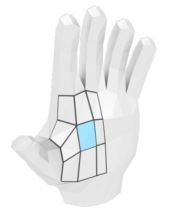
Figure 1: Isogeometric analysis using manifold-based smooth surfaces. The smooth surface in the middle is described by the control mesh on the left and the corresponding manifold basis functions. The deflected geometry on the right is the result of a finite element thin-shell computation with manifold basis functions.

In the present work we follow Ying and Zorin [19] and construct smooth basis functions by combining manifold techniques with conformal parameterisations and partition of unity method. The control mesh consists of quadrilateral elements with some extraordinary vertices (i.e. $v\neq 4$ for some non-boundary vertices) and the construction gives one basis function for each vertex. The first step is to assign each vertex of the control mesh and its adjacent elements a planar sub-mesh with the same connectivity. The sub-meshes serve as control meshes for planar surface patches, which can be understood as parameter spaces for basis functions. For $C^{k}$ continuous basis functions the planar patches have to have a $C^{k}$ smooth parameterisation. Although other choices are conceivable, the patches are parameterised using conformal (angle-preserving) maps. Since each surface point is represented on several patches transition functions composed of conformal maps are used to navigate between adjacent patches. In the second step of the construction, on each planar patch the conventional partition of unity method (PUM) of Melenk et al. [29, 30] is used for constructing basis functions. According to PUM, the basis functions are the product of a partition of unity function and a patch specific polynomial approximant. In computer graphics literature the partition of unity function and the patch specific polynomial basis are usually referred to as the blending function and the embedding function, respectively. We use as partition of unity functions b-splines that have zero value and zero $k-1$ derivatives at the patch boundaries. In order to enforce partition of unity the b-splines on different patches overlapping the same point on the manifold surface are first identified with transition functions and subsequently normalised as in usual PUM. The last step in the basis function construction is to express the local PUM polynomial approximant in dependence of vertex values using a least-squares approximation. In this mesh-based approach the degree of the polynomial approximant and the number of vertices in a sub-mesh are correlated. In order to increase the polynomial degree the sub-meshes are enlarged with mesh refinement by quadrisectioning. The basis functions depend only on the connectivity of the control mesh but not its geometry so that they can be precomputed and tabulated for different valences $v$.

The outline of this paper is as follows. Section 2 reviews the relevant manifold concepts from differential geometry and the partition of unity method. The mesh-based manifold basis functions are introduced in Section 3. First, one-dimensional polygonal control meshes are considered, even though it is straightforward to combine one-dimensional manifolds with the partition of unity method by using simple transition functions. Subsequently, two-dimensional quadrilateral meshes are considered for which conformal maps are used as transition functions. In both dimensions, it is shown how the polynomial coefficients in the partition of unity approximation can be expressed as a linear combination of vertex coefficients. In Section 4 the derived mesh-based basis functions are applied to a number of Poisson and thin-shell problems. Numerical convergence with increasing mesh size on meshes with and without extraordinary vertices is investigated.

2 Preliminaries

2.1 Review of manifold concepts

In the following we provide an informal introduction to differentiable manifolds with the aim to introduce the necessary terminology. For clarity, our discussion is restricted to surfaces, i.e. two-dimensional manifolds, embedded in the three-dimensional Euclidean space $\varmathbb{R}^{3}$. A similar introduction, but oriented more towards geometric modelling, can be found in [31]. The manifold concept is much more general than needed in this paper. A more rigorous discussion is found in most standard differential geometry textbooks, see, e.g., [15, 16].

A regular two-manifold, or surface, $\Omega$ is defined as the set of points in $\varmathbb{R}^{3}$, which can be locally continuously one-to-one mapped onto a set of points in $\varmathbb{R}^{2}$. This definition naturally excludes surfaces with t-joints or isolated points. In applications this is, however, not a major restriction since a geometry, for instance, with a t-joint can be represented as a collection of several manifolds.

By definition on a regular surface $\Omega$ around each point $P$ there is an open region $\Omega_{i}\in\Omega$ that can be mapped to an open planar region $\hat{\Omega}_{i}\in\varmathbb{R}^{2}$, see Figure 2. In line with the partition of unity method terminology, in the following ${\Omega}_{i}$ will be referred to as a patch and $\hat{\Omega}_{i}$ as a planar patch. Furthermore, we denote the function for mapping between two patches with $\bm{\varphi}_{i}:\hat{\Omega}_{i}\rightarrow\Omega_{i}$. On the surface $\Omega$ there are many overlapping patches $\Omega_{i}$ such that

$$\Omega =\bigcup_{i\in\varmathbb{N}}\Omega_{i}$$ (1)

and each point $P$ lies at least on one patch. The pair consisting of $(\hat{\Omega}_{i},\bm{\varphi}_{i})$ is called a chart. The set of all charts $\{(\hat{\Omega}_{i},\bm{\varphi}_{i})\}$ is referred to as an atlas for representing the surface $\Omega$.

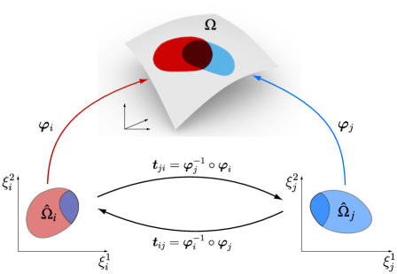
Figure 2: A manifold $\Omega$ and two of the charts $(\hat{\Omega}_{i},\bm{\varphi}_{i})$ and $(\hat{\Omega}_{j},\bm{\varphi}_{j})$ for representing it. A point $P$ in the dark shaded area of the manifold $\Omega$ is represented in both charts and has different coordinates in $\hat{\Omega}_{i}$ and $\hat{\Omega}_{j}$. The change of coordinates between the two charts is given by the transition maps $\bm{t}_{ij}=\bm{t}_{ji}^{-1}$.

As illustrated in Figure 2, each planar patch $\hat{\Omega}_{i}$ has its own coordinate system $\bm{\xi}_{i}=(\xi^{1}_{i},\xi^{2}_{i})$. The same point $P\in\Omega$ in the intersection between the two patches $P\in(\Omega_{i}\cap\Omega_{j})$ has the coordinates $\bm{\xi}_{i}=(\xi^{1}_{i},\xi^{2}_{i})$ in $\hat{\Omega}_{i}$ and $\bm{\xi}_{j}=(\xi^{1}_{j},\xi^{2}_{j})$ in $\hat{\Omega}_{j}$. In order to compute the underlying coordinate transformations we introduce the transition functions

$$\bm{t}_{ji}=\bm{\varphi}_{j}^{-1}\circ\bm{\varphi}_{i}$$ (2)

that are composed out of the mappings $\bm{\varphi}_{j}$. The transition functions are symmetric $\bm{t}_{ij}=\bm{t}_{ji}$ and satisfy the cocyle condition $\bm{t}_{ij}\circ\bm{t}_{ki}=\bm{t}_{kj}$ when the preimage of $P$ lies in three planar patches $\hat{\Omega}_{i}$, $\hat{\Omega}_{j}$ and $\hat{\Omega}_{k}$. For a surface to be $C^{k}$ continuous the transition maps must be $C^{k}$ continuous. Evidently, for a differentiable surface $k$ has to be equal or larger than one.

2.2 Review of the Partition of Unity Method (PUM)

The first use of PUM for creating finite element basis functions goes back to the seminal work of Babuska et al. [32] and was subsequently further developed, for instance, in Melenk et al. [30] and Duarte et al. [33]. In PUM a given domain $\Omega$ in the Euclidean space $\varmathbb{R}^{d}$, with $d\in\{1,2,3\}$, is partitioned into overlapping patches $\Omega_{i}$ such that

$$\Omega =\bigcup_{i\in\varmathbb{N}}\Omega_{i}\,.$$ (3)

As opposed to the manifolds introduced in previous Section 2.1, there is only one single coordinate system in the Euclidean space $\varmathbb{R}^{d}$ and a point $P\in\Omega$ has the same coordinates on $\Omega$ and all patches $\Omega_{i}$. Hence, the transition functions between the different patches are identity maps.

Next, a blending function $w_{i}$ is defined on each patch $\Omega_{i}$. By definition the sum of the blending functions $w_{i}$ over all the regions is

$$\sum_{i}w_{i}=1\,.$$ (4)

The set of blending functions $\{w_{i}\}$ is also referred to as the partition of unity subordinate to the set of open patches $\{\Omega_{i}\}$. As will become clear, in order to obtain smooth PUM basis functions the blending functions $w_{i}$ have to be smooth. In addition, on the region boundaries $\partial\Omega_{i}$ the function value and derivatives of $w_{i}$ have to be zero. After choosing on each patch an arbitrary functions $\hat{w}_{i}$ that have the prerequisite properties they can be normalised to yield a blending function

$$w_{i}=\frac{\hat{w}_{i}}{\sum_{j}\hat{w}_{j}}\,.$$ (5)

In our applications $\hat{w}_{i}$ are usually b-spline basis functions.

On each patch $\Omega_{i}$, in addition to the blending functions $w_{i}$ a local polynomial approximant $f_{i}$ is considered

$$f_{i}=\bm{\alpha}_{i}\cdot\bm{p}_{i}\,,$$ (6)

where ${\bm{p}}_{i}$ is vector containing a complete polynomial basis, $\bm{\alpha}_{i}$ is the corresponding vector of the coefficients and the dot represents their scalar product. For instance, for one-dimensional domains and a monomial basis the two vectors are of the form

$$\bm{\alpha} =\begin{bmatrix}\alpha_{1}&\alpha_{2}&\alpha_{3}&\alpha_{4}&\cdots\end{bmatrix}^{\mathsf{T}}\,$$ (7)

$$\bm{p} =\begin{bmatrix}1&\left(x^{1}\right)^{1}&\left(x^{1}\right)^{2}&\left(x^{1}\right)^{3}&\cdots\end{bmatrix}^{\mathsf{T}}\,.$$ (8)

The global approximant $f$ is the sum of the local approximants $f_{i}$ and their multiplication with the blending functions $w_{i}$, that is,

$$f=\sum_{i}w_{i}f_{i}=\sum_{i}w_{i}\left(\bm{\alpha}_{i}\cdot\bm{p}_{i}\right)\,.$$ (9)

The smoothness of this function depends on the smoothness of $w_{i}$ and $f_{i}$. Since the polynomials in $f_{i}$ are infinitely smooth, the smoothness of $f$ is exclusively controlled by the blending functions $w_{i}$. According to the convergence estimates given in [30], the convergence rates for the approximant $f$ depend on the degree of the polynomial basis $\bm{p}_{i}$ and the constants on the blending functions $w_{i}$ and the layout of the overlaps $\Omega_{i}$.

The illustrative one-dimensional example in Figure 3 showcases the construction of a smooth function using PUM. On each patch $\Omega_{i}$ one single cubic b-spline basis functions is used as $\hat{w}_{i}$ for defining the (normalised) blending function $w_{i}$ according to (5). The support size of a cubic b-spline $\hat{w}_{i}$ is equal to the size of its corresponding patch $\Omega_{i}$. The cubic b-spline is a $C^{2}$ continuous function and at the boundaries of $\Omega_{i}$ its value and first and second derivatives are zero [34]. In addition to the blending functions $w_{i}$, in Figure 3 the local quadratic polynomials $f_{i}$ are also shown. The smooth function $f$ constructed according to (9) is shown in Figure 3(b). It is evident that this curve is by construction $C^{2}$ continuous.

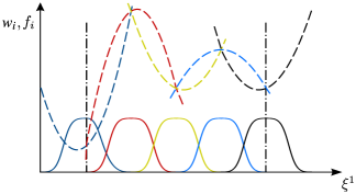
Figure 3: Construction of a smooth function with PUM on a domain with five overlapping patches. On the left the blending functions $w_{i}$ (solid) and the local polynomials $f_{i}$ (dashed) are shown. On the right the obtained smooth function $f$ is shown.

For the considered one-dimensional example, it is straightforward to use a manifold-based approach for constructing the partition of unity function. As shown in Figure 4, the coordinate systems on each patch can be chosen differently. For switching between the different coordinate systems the transition functions $t_{ij}$ are used. In this example one of the chosen transition functions, i.e.  $t_{21}$, is quadratic and the other, i.e. $t_{32}$ ,is linear. It is however possible to chose any other monotone $C^{2}$ function. Choosing other transition functions will lead to a change in the shape of the constructed function $f$.

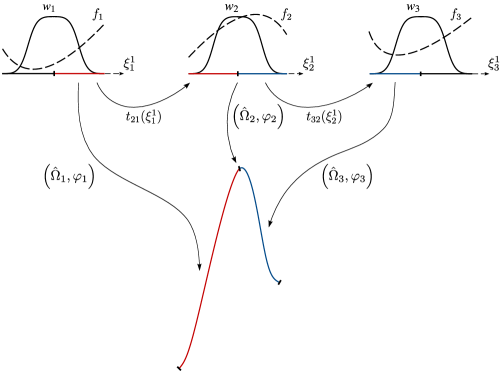
Figure 4: Construction of a smooth function with manifold-based PUM. The domain consists of three overlapping patches (top). On each patch the blending function $w_{i}$ (solid) and the local polynomial $f_{i}$ (dashed) are shown. The transition functions between the overlapping patches are chosen as $t_{21}=-\left(\xi_{1}^{1}\right)^{2}+2\xi_{1}^{1}-1$ and $t_{32}=\xi_{2}^{1}-1$. The obtained smooth function $f$ is shown at the bottom.

3 Mesh-based manifold basis functions

We are now in a position to introduce the construction of manifold-based basis functions on one- and two-dimensional meshes. The idea of using manifolds for smooth interpolation on meshes has been originally introduced in computer graphics by Grimm et al. [17]. The one-dimensional case is straightforward and is only discussed in order to provide some intuition for the two-dimensional case. The essential difficulty in two-dimensions lies in defining suitable transition functions. We use the conformal maps as introduced in Ying and Zorin [19] for defining the transition functions. Alternative definitions have been provided in  [17, 18, 24].

3.1 One-dimensional meshes

First we aim to construct a smooth curve, i.e. a one-dimensional smooth manifold for a given coarse control polygon in the Euclidean space $\varmathbb{R}^{3}$. We begin with defining charts $(\hat{\Omega}_{i},\bm{\varphi}_{i})$ for each vertex, see  Figure 5. The planar patch $\hat{\Omega}_{i}$ is formed from two segments and the attached three vertices. This is usually referred to as the one-ring of the centre vertex. It is also possible to increase the size of $\hat{\Omega}_{i}$ to a two-ring or even larger. The chosen size of the patches influences the number of overlapping patches at each point. As typical for manifolds, each planar patch $\hat{\Omega}_{i}$ has its own coordinate system. The scalar transition functions $t_{ij}$ enable to navigate between the patches $\hat{\Omega}_{i}$ and $\hat{\Omega}_{j}$. The transition functions are chosen as linear maps.

The coordinates of a point $P(x^{1},x^{2},x^{3})$ on the smooth curve is now determined with the partition of unity method. According to (9) we can write, for instance, for the $x^{1}$ coordinate of the point $P$ with a preimage on the planar patch $\hat{\Omega}_{i}$ and coordinate $\xi_{i}$

$$x^{1}(\xi_{i})=\sum_{j}w_{j}(\xi_{i})\left(\bm{\alpha}_{j}^{1}\cdot\bm{p}(\xi_{i})\right)\,.$$ (10)

The summation is over all patches and in order to evaluate the sum it is necessary to use the transition maps. Although we give here and in the following only the expression for $x^{1}$, the other two coordinates $x^{2}$ and $x^{3}$ are expressed similarly. On each one-ring there are three vertices, which motivates the choice of a quadratic basis for $\bm{p}(\xi_{i})$. For a quadratic Lagrangian basis $\bm{L}(\xi_{i})$ the three coefficients are simply the coordinates of the vertices in the one-ring:

$$x^{1}(\xi_{i})=\sum_{j}w_{j}(\xi_{i})\left(\bm{x}_{j}^{1}\cdot\bm{L}(\xi_{i})\right)\,.$$ (11)

Both vectors $\bm{x}_{j}^{1}$ and $\bm{L}(\xi_{i})$ have three components and the entries of $\bm{x}_{j}^{1}$ are the $x^{1}$ coordinates of the three control polygon vertices. This equation is illustrated in Figure 5. As can be seen, the smooth curve passes exactly through the vertices of the control polygon.

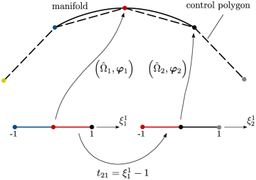
Figure 5: A control polygon (dashed) with the corresponding smooth curve (solid). On each of the two shown one-rings the blending function is a normalised cubic b-spline and the local approximant is a quadratic polynomial.

Next, we rewrite equation (11) in index notation to define basis functions that can be used for finite element analysis:

$$x^{1}(\xi_{i})=\sum_{j}w_{j}(\xi_{i})\left(\sum_{I=1}^{3}x_{j,I}^{1}L_{I}(\xi_{i})\right)=\sum_{I=1}^{3}\left(\sum_{j}w_{j}(\xi_{i})L_{I}(\xi_{i})\right)x_{j,I}^{1}=\sum_{I=1}^{3}N_{I}(\xi_{i})x_{j,I}^{1}\,,$$ (12)

where $N_{I}$ are the three basis functions corresponding to the three vertices in the patch $\hat{\Omega}_{j}$. In Figure 6 the non-zero basis functions and their derivatives in one patch are shown. In the underlying construction the blending functions are normalised cubic b-splines, local polynomials are quadratic and the transition function are linear. Note that the support size of one basis function is two elements. Due to the overlaps there are four non-zero basis functions in one element. The resulting basis functions are $C^{2}$ continuous.

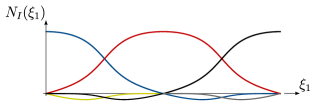
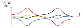
Figure 6: Basis functions (left) and their derivatives (right) in two adjacent elements. In one element there are four non-zero basis functions with two, i.e. the negative ones in the left figure, corresponding to vertices on neighbouring elements.

3.2 Two-dimensional quadrilateral meshes

We now consider the construction of a smooth surface, i.e. smooth two-manifold, for a given coarse control mesh. Our approach follows closely the construction originally introduced in Ying and Zorin [19]. Although only quadrilateral meshes are considered, it is straightforward to extend the technique to triangular meshes.

In addition to the smoothness properties of blending functions and local polynomials, the smoothness of transition functions is central in generating smooth surfaces. For implementation purposes, it is also important that the transition functions and their inverses are readily computable. Similar to the one-dimensional construction, we define charts $(\hat{\Omega}_{i},\bm{\varphi_{i}})$ for each vertex of the mesh. The planar patch $\hat{\Omega}_{i}$ is chosen for now as the one-ring of elements around a vertex. The number of elements in the one-ring of a vertex is referred to as the valence $v$ of the vertex. On structured meshes all vertices inside the domain have valence $v=4$ and on unstructured meshes it can be arbitrary. Hence, in the unstructured case the overlapping one-ring patches can have different valences, which makes the computation of a smooth transition function challenging. Ying et al. [19] proposed conformal maps as smooth and easy computable transition functions. Recall here that conformal mapping is an angle preserving transformation. The generation of a conformal parameterisation for a one-ring of elements proceeds in several steps. In Figure 7 the procedure for a vertex with valence $v=5$ is illustrated. The smooth parameterisation is obtained by conformally mapping, rotating and combining unit squares. The points of the unit square have the coordinates $\bm{\eta}=(\eta^{1},\eta^{2})$ and are expressed as a complex number $z=\eta^{1}+i\eta^{2}$. The conformal transformation $z^{4/v}$ maps the square to a wedge. In computing the mapping recall the following standard relations:

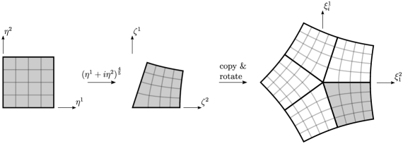
Figure 7: Conformal parameterisation of an one-ring patch with valence $v=5$ (right). The unit square (left) is first conformally mapped to a wedge (middle) with $z^{4/5}=(\eta^{1}+i\eta^{2})^{4/5}$. Subsequently five copies of the wedge are suitably rotated and combined into a one-ring patch.

$$z=\eta^{1}+i\eta^{2}=|z|\left(\cos\phi+i\sin\phi\right)=|z|e^{i\phi}\qquad\text{with }\;|z|=\sqrt{{(\eta^{1})}^{2}+{(\eta^{2})}^{2}}\;\text{ and }\;\phi=\arctan\left(\eta^{2}/\eta^{1}\right)\,.$$ (13)

After the mapping the coordinates $\bm{\eta}=(\eta^{1},\eta^{2})$ of a point become $\bm{\zeta}=(\zeta^{1},\zeta^{2})$ according to:

$$\zeta^{1}+i\zeta^{2}=z^{4/v}=|z|^{4/v}e^{i4\phi/v}\,.$$ (14)

The wedge-shaped image of the conformally mapped unit square forms one sector of the one-ring patch. This wedge is copied and suitably rotated to form a smoothly parameterised one-ring forming patch $\hat{\Omega}_{i}$. The angle preservation property of the conformal map ensures that the parameter lines on $\hat{\Omega}_{i}$ are smoothly connected across element edges, see Figure 7. For the sequence of transformations from the unit square to the smoothly parameterised patch $\hat{\Omega}_{i}$ we abstractly write

$$\bm{\xi}_{i}=\bm{S}_{i}(\bm{\eta})\,,$$ (15)

where the non-linear mapping $\bm{S}_{i}$ is comprised of the conformal transformation $z^{4/v}$ and a rotation. It it worth emphasising that it is straightforward to compute the inverse and derivatives of the mapping (15). Moreover, $\bm{S}_{i}$ depends only on the valence of the considered patch, but not on the vertex coordinates. See Figure 8 for conformal parameterisation of one-ring patches with valences $v\in\{3,4,6\}$.

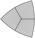
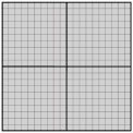
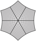
Figure 8: Conformal parameterisations one one-ring patches with valence three (left), four (middle) and six (right). The shown fine meshes represent the parameter lines with either $\eta^{1}=\text{const.}$ or $\eta^{2}=\text{const.}$.

The functions $\hat{w}_{i}$ for computing the normalised blending functions $w_{i}$ are also assembled from smooth functions defined on unit squares. In our computations $\hat{w}_{i}$ is one quarter of a tensor-product b-spline and covers the entire unit square. Figure 9 shows the procedure for constructing the blending function on a valence five patch. It can be seen that the b-spline has its maximum at the corner which maps to the central vertex of the one-ring patch $\hat{\Omega}_{i}$. To normalise the functions $\hat{w}_{i}$, for a given point on patch $\hat{\Omega}_{i}$ the corresponding point on an overlapping patch $\hat{\Omega}_{j}$ is computed with transition functions, that is, $\bm{\xi}_{j}=(\bm{S}_{j}\circ\bm{S}_{i}^{-1})(\bm{\xi}_{i})$, cf. (15). The blending function is then first mapped onto the conformal wedge and then appropriately rotated to construct the blending function on the patch. In Figure 10 the normalised blending functions for one-ring patches with $v\in\{3,4,6\}$ are shown.

In [19] the weight functions $w_{i}$ are chosen such that they are constant in a small neighbourhood of width $\delta$ close to the unit square boundaries. This is motivated by the need to circumvent the singularity of the conformal map at the central vertex of the one-ring patch. Our numerical experiments indicate that the finite element solutions are insensitive to the choice of $\delta$ so that $\delta=0$ is chosen. Note that for evaluating the finite element integrals the surface is only evaluated at quadrature points, which are usually away from the vertices. Alternatively, the one-ring patches can also be parameterised with the characteristic map of Catmull-Clark subdivision surfaces, which is $C^{2}$ smooth and does not have a singularity at the extraordinary vertex, see [24, 22] for details.

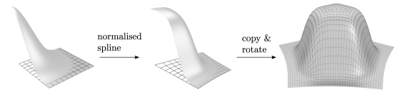
Figure 9: One quarter of a tensor-product cubic b-spline as the non-normalised blending function $\hat{w}_{i}$ on the unit square (left). Normalised blending function $w_{i}$ on the conformal wedge (middle) and on a conformal patch with valence five (right).

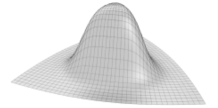
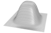
Figure 10: Blending functions $w_{i}$ for one-ring patches with valence three (left), four (middle) and six (right). The shown fine meshes represent the parameter lines with either $\eta^{1}=\text{const.}$ or $\eta^{2}=\text{const.}$.

We now proceed to the construction of a smooth surface, i.e. a two-dimensional smooth manifold, for a given coarse control mesh. The overall approach is very similar to the one-dimensional case introduced in the previous section. We consider again a point $P(x^{1},x^{2},x^{3})$ on the manifold with a preimage with the coordinates $\bm{\xi}_{i}$ on the planar patch $\hat{\Omega}_{i}$. Each of the coordinate components of $P$ are interpolated with the partition of unity method. We write, for instance, for the $x^{1}$ coordinate

$$x^{1}(\bm{\xi}_{i})=\sum_{j}w_{j}(\bm{\xi}_{i})\left(\bm{\alpha}_{j}^{1}\cdot\bm{p}(\bm{\xi}_{i})\right)\,,$$ (16)

where $\bm{p}(\bm{\xi})$ is a vector containing the components of a polynomial basis and $\bm{\alpha}_{j}^{1}$ are the unknown coefficients. Next, the coefficients $\bm{\alpha}_{j}^{1}$ are expressed in dependence of the vertex coordinates of the control mesh. The dimension of the polynomial basis has to be equal or smaller than the number of vertices in a patch $\hat{\Omega}_{j}$. Because on unstructured meshes the valence of vertices is not fixed, we choose a polynomial basis based on the one-ring with the smallest valence in the mesh. If a higher degree polynomial is desired, two or more rings of elements can be considered as patches $\hat{\Omega}_{j}$. When the dimension of the polynomial basis is smaller than the number of vertices in the patch $\hat{\Omega}_{j}$, the polynomial coefficients $\bm{\alpha}_{j}^{1}$ are determined with a local least-squares projection on each patch. Neglecting for the moment the patch index, and denoting the parametric coordinates of the $2v+1$ vertices on patch $\hat{\Omega}_{i}$ as $\bm{\xi}_{I}$ and the corresponding nodal control mesh coordinates as $x_{I}^{1}$, the least-squares fit on $\hat{\Omega}_{j}$ reads

$$\left(\sum_{I=1}^{2v+1}\bm{p}(\bm{\xi}_{I})\bm{p}^{\mathsf{T}}(\bm{\xi}_{I})\right)\bm{\alpha}^{1}=\sum_{I=1}^{2v+1}\bm{p}(\bm{\xi}_{I})x_{I}^{1}\,.$$ (17)

Note for a specific polynomial basis the matrix on the left hand side depends only on the valence of the one-ring and can be precomputed and stored. We abbreviate the least-squares projection (17) with

$$\bm{\alpha}^{1}=\bm{A}\bm{x}^{1}\,,$$ (18)

where $\bm{A}$ is the projection matrix and the vector $\bm{x}^{1}$ contains the $x^{1}$ coordinates of all the vertices in the one-ring, i.e. on the planar patch.

Finally, by making use of (18) we can write the partition of unity interpolation (16) in dependence of the vertex coordinates of the control mesh

$$x^{1}(\bm{\xi}_{i}) =\sum_{j}w_{j}(\bm{\xi}_{i})\left(\bm{p}(\bm{\xi}_{i})\cdot\bm{A}\bm{x}_{j}^{1}\right)=\sum_{j}w_{j}(\bm{\xi}_{i})\sum_{I=1}^{2v+1}\left(\bm{p}(\bm{\xi}_{i})\cdot\bm{A}\right)_{I}x_{j,I}^{1}$$ (19)

$$=\sum_{I=1}^{2v+1}\sum_{j}\left(w_{j}(\xi_{i})\left(\bm{p}(\bm{\xi}_{i})\cdot\bm{A}\right)_{I}\right)x_{j,I}^{1}=\sum_{I=1}^{2v+1}N_{I}(\bm{\xi}_{i})x_{j,I}^{1}\,.$$

This gives rise to the definition of basis functions $N_{I}(\xi_{i})$, where $I$ is the vertex id on patch $\hat{\Omega}_{j}$. In conventional finite element implementations usually system matrices and vectors are evaluated by iterating over the elements in the control mesh. Moreover, during numerical integration the basis function values at pretabulated points in the integration element are needed. In manifold finite elements the unit square in the  $\eta^{1}-\eta^{2}$ coordinate system is chosen as the integration element. Hence, the basis functions $N_{I}(\bm{\xi}_{i})$ have to be evaluated in a given element and integration point $\bm{\eta}=(\eta^{1},\eta^{2})$.

We briefly consider the hand geometry shown in Figure 1 for illustrating the process of evaluating the basis functions; see A for more details. On the control mesh in Figure 1 (left) one element is highlighted and the four one-rings belonging to its four vertices are indicated. One of the element’s vertices has valence $v=5$ and the other three have valence $v=4$. The interpolation within the highlighted element depends on the eighteen vertices in the union of the four one-rings. In Figure 11 the four patches used for partition of unity construction are shown. The unit square in the centre represents the integration element, equivalent to the parent element in isoparametric finite elements. The conformal mapping $\bm{S}_{i}(\bm{\eta})$ of the unit square to the four planar one-ring patches $\hat{\Omega}_{i}$ depends on the valence of the respective one-ring. For the three patches with valence four, the mapping is (up to some rotations) essentially an identity map. With the transition maps implied by the mappings $\bm{S}_{i}$ it is straightforward to compute the basis functions defined in (19) for a given integration point $\bm{\eta}_{Q}=(\eta^{1}_{Q},\eta^{2}_{Q})$. In this specific example the minimum number of vertices in a patch is nine so that the polynomial basis $\bm{p}(\bm{\xi}_{i})$ can be chosen either as a bilinear or biquadratic Lagrangian basis. Note that on patches with valence $v=4$ and a biquadratic Lagrangian basis the least-squares projection matrix $\bm{A}$ is an identity matrix. Moreover, as also can be deduced from Figure 11 each basis function $N_{I}$ has a support size consisting of two rings of elements around its associated vertex. In Figure 12 basis functions for vertices with valence $v\in\{3,4,6\}$ are shown.

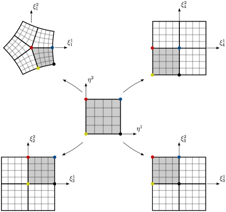
Figure 11: One integration element (centre) and its overlapping four conformally parameterised planar patches. The integration element represents the highlighted blue element in the hand control mesh shown in Figure 1 (left).

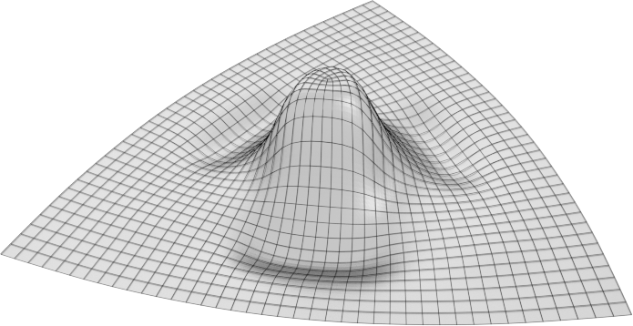
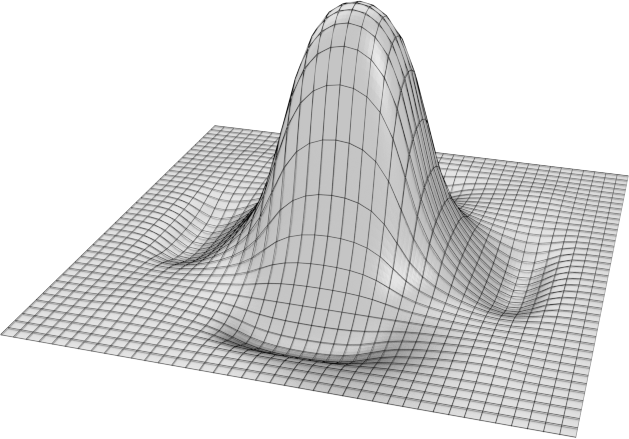
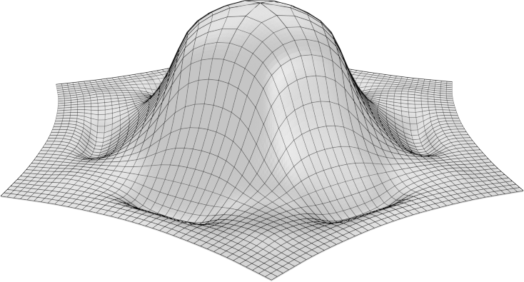
Figure 12: Basis functions for vertices with valence three (left), four (middle) and six (right). The shown fine meshes represent the parameter lines with either $\eta^{1}=\text{const.}$ or $\eta^{2}=\text{const.}$.

4 Examples

We consider second and fourth-order partial differential equations to demonstrate the accuracy and convergence of the introduced manifold basis functions when used in finite element analysis. For manifold construction, around each vertex patches consisting of either one or two-rings of elements are considered. As blending functions we use either normalised linear, quadratic or cubic b-splines. The element integrals are evaluated with $9\times 9$ Gauss integration points in all examples. This high number of integration points has been chosen in order to minimise the effect of integration errors. In convergence studies the control meshes are refined with the Catmull-Clark subdivision scheme [35]. The number of extraordinary vertices in a mesh remains constant because the new vertices introduced during the refinement are all ordinary.

Surfaces with boundaries require modified charts for manifold constructions, such as those introduced in [36]. The specialised treatment of elements close to the boundary can be avoided by introducing ghost elements just outside the domain. This is achieved by reflecting sufficient number of internal elements and vertices along the boundary. Furthermore, the manifold basis functions are non-interpolating at the boundaries. Therefore, we use the penalty method for applying Dirichlet boundary conditions.

4.1 Two-dimensional Poisson problems

4.1.1 Square domain with a structured mesh

As an introductory example, we solve the Poisson-Dirichlet problem $-\nabla\cdot\nabla\bm{u}=q$ on the domain $\Omega=(0,1)\times(0,1)$, discretised with a Cartesian grid, see Figure 13. The loading $q$ is chosen such that the analytical solution is

$$u(\bm{\mathrm{x}})=\cos(4\pi x^{1})\cos(4\pi x^{2})\,,$$ (20)

where the variables $\bm{x}=(x^{1},x^{2})$ represent coordinates.

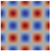
Figure 13: Structured coarse control mesh (left) and contour plot of the solution $u^{h}$ (right, using a finer control mesh).

In the partition of unity construction we use a biquadratic Lagrangian basis as the local polynomial basis $\bm{p}(\bm{\xi}_{i})$ and as blending functions $w(\bm{\xi}_{i})$ we consider normalised linear, quadratic and cubic b-splines. To begin with, the number of Gauss points required for adequate integration is determined, see Figure 14. In Figure 14 only normalised cubic b-splines are used. Since the basis functions are rational, a large number of Gauss points is unavoidable, especially for finer meshes. Furthermore, our findings indicate that blending functions with higher continuity, in general, require more Gauss points. According to Figure 14, the chosen $9\times 9$ Gauss points for all examples in the paper seems to provide a good trade-off between accuracy and efficiency.

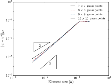
Figure 14: Square domain with a structured mesh. Influence of number of Gauss integration points on $L^{2}$ norm error. The local polynomial basis $\bm{p}$ is quadratic and the blending functions $w_{i}$ are normalised cubic b-splines.

Figure 15 shows the $L^{2}$ norm and $H^{1}$ semi-norm of error $u-u^{h}$ as the mesh is uniformly refined with the Catmull-Clark scheme. For this structured mesh Catmull-Clark refinement is equivalent to refinement by bisection. The error norms for three different blending functions, namely normalised linear, quadratic and cubic splines, are shown. It can be inferred from these convergence plots that the convergence rates are optimal and are unaffected by the blending functions. Interestingly, the constants in the convergence plots increase when the smoothness of the blending function is increased.

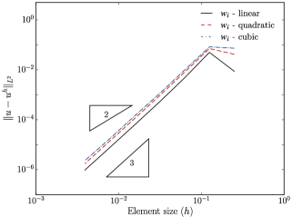
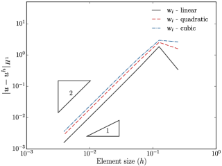
Figure 15: Square domain with a structured mesh. Convergence of the $L^{2}$ norm (left) and $H^{1}$ (right) semi-norm errors. The local polynomial basis $\bm{p}$ is quadratic and the blending functions $w_{i}$ are normalised linear, quadratic or cubic b-splines.

4.1.2 Square domain with an unstructured mesh

This example underlines the performance of manifold basis functions on unstructured meshes, and studies how the convergence rates are influenced in the presence of extraordinary vertices. To this end, the Poisson-Dirichlet problem with the analytical solution

$$u(\bm{\mathrm{x}})=\sin(4\pi x^{1})\sin(4\pi x^{2})$$ (21)

is considered. Figure 16 shows the unstructured mesh used in the computations and a representative finite element solution. The mesh lines on the displaced solution in Figure 16 represent the edges of the elements on the exact surface. The mesh has eight extraordinary vertices, with four vertices of valence $v=3$ and the other four of valence $v=5$.

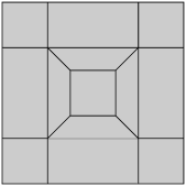
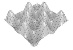
Figure 16: Unstructured coarse control mesh (left) and the finite element solution (right).

In the convergence studies we use as local polynomials $\bm{p}(\bm{\xi}_{i})$ bilinear and biquadratic Lagrangian polynomials. As patches one- and two-rings of elements are considered. However, in one-ring patches with valence $v=3$ there are only seven vertices so that instead of a biquadratic Lagrangian polynomial locally a complete quadratic polynomial has to be used. In all cases the blending functions $w(\bm{\xi}_{i})$ are normalised cubic b-splines.

Figure 17 shows the $L^{2}$ norm and $H^{1}$ semi-norm of the error $u-u^{h}$ as the mesh is successively refined with the Catmull-Clark scheme. It can be seen that for all cases, the convergence rates are close to optimal. In the $L^{2}$ norm and for quadratic polynomials  ($\mu=2$) the convergence rates for one- and two-ring patches are approximately $2.9$ and $2.7$ respectively. In the $H^{1}$ semi-norm, the corresponding convergence rates are $1.9$ and $1.7$ respectively. We believe that the reduction of convergence rates with increasing patch size is primarily due to the suboptimal integration of rational polynomials.

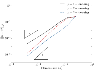
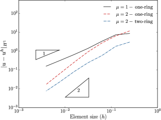
Figure 17: Square domain with an unstructured mesh. Convergence of the $L^{2}$norm (left) and $H^{1}$ (right) semi-norm errors. The local polynomial basis $\bm{p}$ is either linear ($\mu=1$) or quadratic ($\mu=2$) and the blending functions $w_{i}$ are normalised cubic b-splines.

Next, we study the pointwise convergence of the solution at selected vertices. For this part of the studies we use one- and two-ring patches and consider only biquadratic Lagrangian polynomials. As mentioned before for one-ring patches with valence $v=3$ instead of the biquadratic Lagrangian a complete quadratic has to be used. The blending functions are normalised cubic b-splines. Figure 18 (left) shows the convergence of the error at three selected vertices with valences $v\in\{3,4,5\}$ when one-ring patches are used. Figure 18 (right) shows the corresponding plots when two-ring patches are used. For both types of patches, the convergence rate at extraordinary vertices is $2$. It is interesting to note that two-ring patches, in general, have smaller errors than the one-ring patches.

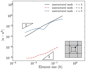
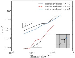
Figure 18: Square domain with an unstructured mesh. Pointwise convergence of the solution at three selected vertices with valences $v\in\{3,4,5\}$ for one-ring (left) and two-ring patches (right). The local polynomial basis $\bm{p}$ is quadratic and the blending functions $w_{i}$ are normalised cubic b-splines.

4.1.3 Circular domain

In this example the Poisson-Dirichlet problem with the same solution as in (21) is solved on a circular domain with radius $||x||<0.5$, see Figure 19. The aim is to illustrate the treatment of curved boundaries when manifold basis functions are used. As previously mentioned, in our present implementation, ghost nodes are introduced at the boundaries, which circumvents the use of modified charts close to the boundaries. With specialised boundary charts the treatment of boundaries would be different.

Figure 19 (left) shows the coarse mesh containing four extraordinary vertices with valence $v=3$. The domain boundary is approximated by least-squares fitting an approximate circle described by the manifold basis functions to the exact circle. In the least-squares problem the unknowns are the positions of the vertices close to the boundary. This is performed as a preprocessing step each time after the mesh is refined with Catmull-Clark subdivision.

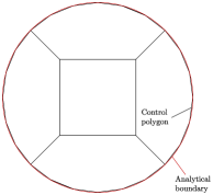
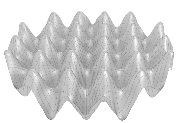
Figure 19: Exact and approximated circular domains and the coarse control mesh (left) and finite element solution (right).

In the convergence study shown in Figure 20 only one-ring patches are used. The local polynomials $\bm{p}(\bm{\xi}_{i})$ are either biquadratic Lagrangian polynomials for patches with valence $v\neq 3$ or complete quadratic polynomials for patches with $v=3$. The blending functions $w(\bm{\xi}_{i})$ are normalised cubic b-splines. As can be inferred from Figure 20, optimal convergence rates for the $L^{2}$ norm and the $H^{1}$ semi-norm error are achieved.

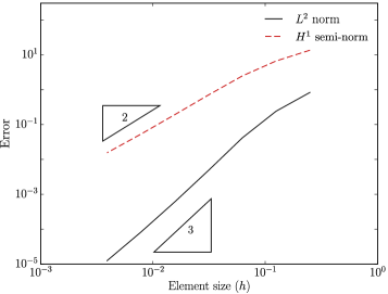
Figure 20: Circular domain. Convergence of the $L^{2}$ norm and $H^{1}$ semi-norm errors. The local polynomial basis $\bm{p}$ is quadratic and the blending functions $w_{i}$ are normalised cubic b-splines.

4.2 Thin-plate and thin-shell problems

The linear Kirchhoff-Love model is used for computing the thin-plate and thin-shell problems introduced in the following. The corresponding weak form depends on the metric and curvature tensors of the mid-surface in the reference and deformed configurations. Due to the presence of the curvature tensor, the basis functions have to be smooth, or more precisely in space $H^{2}$. The presented computations have been performed by replacing the subdivision basis functions in our software [12, 37] with manifold-basis functions. Due to the algorithmic similarities between subdivision and manifold basis functions it is straightforward to replace one with the other. Out-of-plane shear deformations have been neglected although it would be possible to take them into account as proposed in [37].

4.2.1 Simply supported square plate

We consider the deformation of a simply supported square plate of unit length subjected to an applied pressure loading $q=10000$. The thickness of the plate is $h=0.01$, the Young’s modulus is $E=70\times 10^{9}$, and the Poisson ratio is $\nu=0.3$. Its analytical solution according to [38] is

$$u(\bm{\mathrm{x}})=\frac{16q}{\pi^{6}D}\sum_{i=1}^{\infty}\sum_{j=1}^{\infty}\frac{\sin(i\pi x^{1})\sin(j\pi x^{2})}{ij(i^{2}+j^{2})^{2}}\,,$$ (22)

where $D=Eh^{3}/(12(1-\nu^{2})$ is the flexural rigidity.

The unstructured mesh shown in Figure 16, previously used for the Poisson-Dirichlet problem, is reused for this plate problem. Recall that the mesh has eight extraordinary vertices, namely four with $v=3$ and the other four with $v=5$. In the convergence study, one-rings and two-rings of elements are considered. Except on valence $v=3$ one-ring patches, the local polynomials $\bm{p}(\bm{\xi}_{i})$ are biquadratic Lagrangian polynomials. As previously mentioned, on one-ring patches with $v=3$ only a complete quadratic polynomial can be used, because there are only seven vertices in a patch. In all cases the blending function $w(\bm{\xi}_{i})$ is a normalised cubic b-spline. In Figure 21 (left), the deflected shape of the simply-supported plate for a relatively coarse mesh is shown. Figure 21 (right) illustrates the convergence of the $L^{2}$ norm error as the mesh is successively refined with the Catmull-Clark scheme. The constant in the convergence plot decreases with increasing patch size. For both patch sizes, the convergence rate is approximately $1.7$, which is slightly lower than the optimum of $2$. One possible reason for this is the inadequate integration of the rational polynomials.

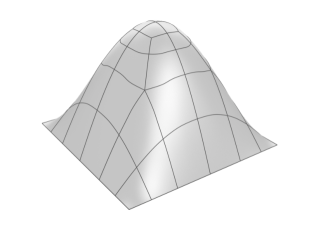
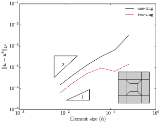
Figure 21: Simply supported square plate. Deflected plate (left) and convergence of the $L^{2}$ norm error (right). The local polynomial basis $\bm{p}$ is quadratic and the blending functions $w_{i}$ are normalised cubic b-splines.

4.2.2 Pinched cylinder

The pinched cylinder is one of the benchmark examples for shell finite elements suggested in Belytschko et al. [39]. The unstructured coarse control mesh, material properties and the general problem setup are shown in Figure 22 (left). The ends of the cylinder are unconstrained and the two diametrically opposite forces are applied within the middle section of the cylinder.

Figure 22: Definition of the pinched cylinder problem (left) and deformed pinched cylinder (right).

The deflected pinched cylinder is shown in Figure 22 (right). In Figure 23 the convergence of the normalised maximum change in diameter of the Catmull-Clark and manifold finite element solutions are compared, both structured and unstructured meshes are considered. The change in diameter is normalised with the exact solution $4.52\times 10^{-4}$ for a membrane shell given in [38]. It can be seen that the Catmull-Clark and manifold solutions converge to very similar values. The convergence of manifold functions with cubic polynomials ($\mu=3$) on two-ring patches is comparable with subdivision basis functions. Note that for structured meshes Catmull-Clark subdivision basis functions are identical to tensor-product cubic b-splines [9]. The slower convergence of the manifold basis functions with quadratic polynomials ($\mu=2$) on one-ring patches is as expected.

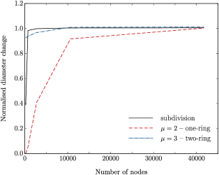
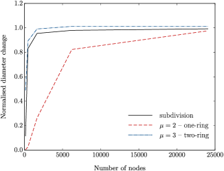
Figure 23: Pinched cylinder. Convergence of maximum change in diameter with manifold and Catmull-Clark basis functions for structured (left) and unstructured (right) meshes. The local polynomial basis $\bm{p}$ is either quadratic ($\mu=2$) or cubic ($\mu=3$) and the blending functions $w_{i}$ are normalised cubic b-splines.

4.2.3 Pinched hemisphere

Our last example is the pinched hemisphere, which has also been suggested in Belytschko et al. [39] as a benchmark for shell finite elements. The coarse control mesh, material properties and the general problem setup are shown in Figure 24 (left). The edge of the hemisphere is unconstrained and the four radial forces have alternating signs. The sum of the applied forces is zero. In the control mesh the valence of the vertices range between 3 and 5.

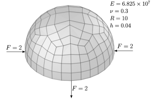
Figure 24: Definition of the pinched hemisphere problem (left) and deformed pinched hemisphere (right).

The deformed surface of the pinched hemisphere is shown in Figure 24 (right). Figure 25 shows the convergence of the normalised maximum radial displacement. The displacements are normalised by $0.0924$, given in Belytschko et al. [39]. The same plot also includes the convergence of the finite element solution when Catmull-Clark basis functions are used. As in case of pinched cylinder example, the manifold basis functions are constructed with quadratic local polynomials ($\mu=2$) on one-rings and cubic polynomials ($\mu=3$) on two-ring patches. In both cases, normalised cubic b-splines were used as blending functions. Figure 25 illustrates that the manifold basis functions constructed using cubic polynomial patches converges slightly faster than the Catmull-Clark subdivision basis functions.

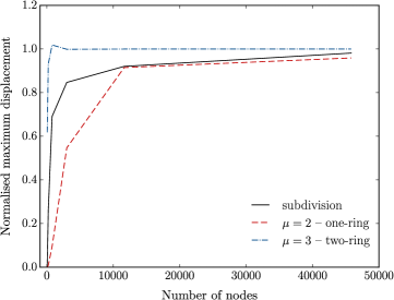
Figure 25: Pinched hemisphere. Convergence of maximum radial displacement with manifold and Catmull-Clark basis functions. The local polynomial basis $\bm{p}$ is either quadratic ($\mu=2$) or cubic ($\mu=3$) and the blending functions $w_{i}$ are normalised cubic b-splines.

5 Conclusions

We introduced an isogeometric analysis technique that uses manifold smooth basis functions on quadrilateral meshes. Manifold techniques have a long history in computer graphics and computer aided design and several variants have been proposed over the years. Our implementation closely follows Ying and Zorin [19] and combines manifold techniques with conformal parameterisations and the partition of unity method. The smoothness of the basis functions is determined by the smoothness of the blending, or partition-of-unity, functions. The approximation properties of the basis functions is mainly determined by the polynomial degree used in each patch. In the presented computations, the blending function was chosen either as a normalised linear, quadratic or cubic b-spline leading to $C^{0}$, $C^{1}$ or $C^{2}$ continuous basis functions, respectively. As patch sizes for the manifold construction, one- or two-ring layers of elements around a vertex were considered. The number of vertices in a patch determines the maximum degree of the local polynomial that can be used in the partition-of-unity interpolation. The polynomial coefficients in the partition of unity interpolation are expressed as vertex coefficients using a least-squares procedure. The finally obtained basis functions are smooth, rational, locally supported and are associated to vertices in the mesh (similar to b-splines of odd degree). The near optimal convergence of the introduced basis on meshes with extraordinary vertices could be numerically confirmed.

For future research the combination of manifold basis functions with b-splines and the related NURBS or subdivision surfaces appears especially promising. B-splines have several compelling properties, including refinability, that make them ideal for geometric modelling and numerical analysis on meshes with no extraordinary vertices. However, most b-spline techniques for dealing with extraordinary vertices, including subdivision and many $G^{k}$ constructions, do not lead to optimally convergent finite elements [13, 6, 7]. In contrast, as numerically demonstrated manifold basis functions yield nearly optimally convergent finite elements independent of the connectivity of the mesh. This suggests to use b-splines in most of the domain and to introduce manifold basis functions only around extraordinary vertices. In subdivision surfaces manifold techniques have already been used to obtain $C^{2}$ continuity around extraordinary vertices [22, 23, 24]. In these three papers, instead of the conformal map the characteristic map of subdivision surfaces is used to parameterise the planar patches. The advantage of the characteristic map, in comparison to the conformal map, is that it provides a more uniform parameterisation and does not have a singularity at the extraordinary vertex. Additional directions for future research include the mathematical convergence analysis and the proof of the linear independence of the introduced manifold basis function. To this end, the large number of results for partition of unity methods provide a good starting point.

Appendix A Implementation

In the following we discuss the implementation of manifold basis functions focusing on data structures and algorithms. For clarity, the discussion is restricted to the case of patches $\hat{\Omega}_{i}$ consisting of one-ring elements. This section should be read in conjunction with Section 3.2 and specifically Figure 11. In line with conventional finite element implementations it is assumed that the element matrices and vectors are assembled by iterating over elements. For computing the element matrices and vectors the basis function values and derivatives at integration points are required. The basis functions depend only on the connectivity of the mesh but not on the coordinates of the vertices. Hence, they can be precomputed as part of a preprocessing step and stored for later use.

The construction of the manifold basis functions proceeds in several steps. First, for each (non-boundary) vertex in the mesh the elements and vertices in its one-ring are identified. Recall that we introduced one layer of ghost elements just outside the domain of interest and that the charts which belong to the boundary vertices do not intersect the domain. The elements and vertices in an one-ring can efficiently be identified, for instance, using a half-edge data structure.

Following the assembly of the one-rings, we endow each patch $\hat{\Omega}_{j}$ with a blending function $w_{j}(\bm{\xi})$ and a local polynomial basis $\bm{p}(\bm{\xi})$. The degree of $\bm{p}(\bm{\xi})$ is chosen such that it is equal or less than the number of the vertices in the corresponding one-ring, i.e., $2v+1$, where $v$ is the valence of the centre vertex. Subsequently, the basis functions $N_{I}(\bm{\eta}_{Q})$ and their derivatives $\nabla_{\bm{\eta}}N_{I}(\bm{\eta}_{Q})$ for each quadrature (or, Gauss) point $\bm{\eta}_{Q}=(\eta^{1}_{Q},\eta^{2}_{Q})$ in an element $\Box_{i}$ are precomputed. Each four-noded element in the mesh lies within the overlap of four patches, hence, with each $N_{I}(\bm{\eta}_{Q})$ receiving four contributions. The contribution of one patch $\hat{\Omega}_{j}$ to $N_{I}(\bm{\eta}_{Q})$ belonging to the vertex $I$ is computed as follows:

1. Determine the conformal coordinate $\bm{\zeta}_{Q}$ by applying the conformal map $z(\bm{\zeta}_{Q})=z(\bm{\eta}_{Q})^{4/v}$.

2. Identify the image of the considered element $\Box_{i}$ in the patch $\hat{\Omega}_{j}$ by comparing vertex ID’s. Based on that determine the coordinate $\bm{\xi}_{Q}$ in $\hat{\Omega}_{j}$ by applying the rotation

   $$\bm{\xi}_{Q}=\bm{R}\bm{\zeta}_{Q}\,,$$

   where the rotation $\bm{R}$ is a multiple of $2\pi/v$.

3. Compute the contribution of patch $\hat{\Omega}_{j}$ to basis function $N_{I}(\bm{\eta}_{Q})$ according to (19)

   $$w_{j}(\bm{\xi}_{Q})\sum_{k}^{2v+1}p_{k}(\bm{\xi}_{Q})A_{kI}\,,$$

   where the summation is over the components in the polynomial basis $p_{k}(\bm{\xi}_{Q})$. We choose for $p_{k}(\bm{\xi}_{Q})$ either a monomial or a Lagrangian basis. The matrix $A_{kI}$, which is the inverse of the least-squares matrix, does not depend on the coordinates and can be precomputed for all possible valences and stored. For computing the contribution of patch $\hat{\Omega}_{j}$ to the derivatives $\nabla_{\bm{\eta}}N_{I}(\bm{\eta}_{Q})$ the above equation is differentiated, i.e.,

   $$\nabla_{\bm{\eta}}w_{j}=\nabla_{\bm{\xi}}w_{j}\bm{R}^{\mathsf{T}}\left(\frac{\partial\bm{\eta}}{\partial\bm{\zeta}}\right)^{-1}\,.$$

After summing up the contributions of the four overlapping charts, the basis functions, their derivatives and corresponding vertices are stored in maps. The number of (non-zero) basis functions in an element is equal to the number of unique vertices in the union of the element’s four charts.

References

- Hughes et al. [2005] T. J. R. Hughes, J. A. Cottrell, Y. Bazilevs, Isogeometric analysis: CAD, finite elements, NURBS, exact geometry and mesh refinement, Computer Methods in Applied Mechanics and Engineering 194 (2005) 4135–4195.
- Cottrell et al. [2009] J. Cottrell, T. Hughes, Y. Bazilevs, Isogeometric Analysis: Toward Integration of CAD and FEA, John Wiley & Sons Ltd., 2009.
- Bazilevs et al. [2010] Y. Bazilevs, V. M. Calo, J. A. Cottrell, J. A. Evans, T. J. R. Hughes, S. Lipton, M. A. Scott, T. W. Sederberg, Isogeometric analysis using T-splines, Computer Methods in Applied Mechanics and Engineering (2010) 229–263.
- Cirak et al. [2002] F. Cirak, M. Scott, E. Antonsson, M. Ortiz, P. Schröder, Integrated modeling, finite-element analysis, and engineering design for thin-shell structures using subdivision, Computer-Aided Design 34 (2002) 137–148.
- Groisser and Peters [2015] D. Groisser, J. Peters, Matched -constructions always yield -continuous isogeometric elements, Computer Aided Geometric Design 34 (2015) 67–72.
- Nguyen et al. [2014] T. Nguyen, K. Karčiauskas, J. Peters, A comparative study of several classical, discrete differential and isogeometric methods for solving Poisson’s equation on the disk, Axioms 3 (2) (2014) 280–299.
- Nguyen et al. [2016] T. Nguyen, K. Karčiauskas, J. Peters, finite elements on non-tensor-product 2d and 3d manifolds, Applied Mathematics and Computation 272 (2016) 148–158.
- Scott et al. [2013] M. A. Scott, R. N. Simpson, J. A. Evans, S. Lipton, S. P. A. Bordas, T. J. R. Hughes, T. W. Sederberg, Isogeometric boundary element analysis using unstructured T-splines, Computer Methods in Applied Mechanics and Engineering (2013) 197–221.
- Peters and Reif [2008] J. Peters, U. Reif, Subdivision Surfaces, Springer Series in Geometry and Computing, Springer, 2008.
- Zorin and Schröder [2000] D. Zorin, P. Schröder, Subdivision for Modeling and Animation, SIGGRAPH 2000 Course Notes, 2000.
- Cirak et al. [2000] F. Cirak, M. Ortiz, P. Schröder, Subdivision surfaces: A new paradigm for thin-shell finite-element analysis, International Journal for Numerical Methods in Engineering 47 (2000) 2039–2072.
- Cirak and Long [2011] F. Cirak, Q. Long, Subdivision shells with exact boundary control and non-manifold geometry, International Journal for Numerical Methods in Engineering 88 (2011) 897–923.
- Jüttler et al. [2016] B. Jüttler, A. Mantzaflaris, R. Perl, M. Rumpf, On numerical integration in isogeometric subdivision methods for PDEs on surfaces, Computer Methods in Applied Mechanics and Engineering 302 (2016) 131–146.
- Wei et al. [2015] X. Wei, Y. Zhang, T. J. R. Hughes, M. A. Scott, Truncated hierarchical Catmull–Clark subdivision with local refinement, Computer Methods in Applied Mechanics and Engineering 291 (2015) 1–20.
- do Carmo [1976] M. P. do Carmo, Differential geometry of curves and surfaces, Prentice-Hall, Englewood Cliffs, NJ, 1976.
- Schutz [1980] B. F. Schutz, Geometrical methods of mathematical physics, Cambridge University Press, Cambridge, UK, 1980.
- Grimm and Hughes [1995] C. M. Grimm, J. F. Hughes, Modeling surfaces of arbitrary topology using manifolds, in: SIGGRAPH 1995 Conference Proceedings, 359–368, 1995.
- Navau and Garcia [2000] J. C. Navau, N. P. Garcia, Modeling surfaces from meshes of arbitrary topology, Computer Aided Geometric Design 17 (2000) 643–671.
- Ying and Zorin [2004] L. Ying, D. Zorin, A simple manifold-based construction of surfaces of arbitrary smoothness, in: SIGGRAPH 2004 Conference Proceedings, 271–275, 2004.
- Gu et al. [2006] X. Gu, Y. He, H. Qin, Manifold splines, Graphical Models 68 (2006) 237–254.
- Della Vecchia et al. [2008] G. Della Vecchia, B. Jüttler, M.-S. Kim, A construction of rational manifold surfaces of arbitrary topology and smoothness from triangular meshes, Computer Aided Geometric Design 25 (2008) 801–815.
- Levin [2006] A. Levin, Modified subdivision surfaces with continuous curvature, in: SIGGRAPH 2006 Conference Proceedings, 1035–1040, 2006.
- Zorin [2006] D. Zorin, Constructing curvature-continuous surfaces by blending, in: Proceedings of the fourth Eurographics symposium on Geometry processing, 31–40, 2006.
- Antonelli et al. [2013] M. Antonelli, C. V. Beccari, G. Casciola, R. Ciarloni, S. Morigi, Subdivision surfaces integrated in a CAD system, Computer-Aided Design 45 (2013) 1294–1305.
- Levin [2004] D. Levin, Mesh-independent surface interpolation, in: Geometric Modeling for Scientific Visualization, Springer, 37–49, 2004.
- Pauly et al. [2002] M. Pauly, M. Gross, L. P. Kobbelt, Efficient simplification of point-sampled surfaces, in: Proceedings of the conference on Visualization’02, 163–170, 2002.
- Millán et al. [2010] D. Millán, A. Rosolen, M. Arroyo, Thin shell analysis from scattered points with maximum-entropy approximants, International Journal for Numerical Methods in Engineering 85 (2010) 723–751.
- Millán et al. [2013] D. Millán, A. Rosolen, M. Arroyo, Nonlinear manifold learning for meshfree finite deformation thin-shell analysis, International Journal for Numerical Methods in Engineering 93 (2013) 685–713.
- Melenk [1995] J. M. Melenk, On generalized finite element methods, Ph.D. thesis, The University of Maryland, 1995.
- Melenk and Babuska [1996] J. M. Melenk, I. Babuska, The partition of unity finite element method: Basic theory and applications, Computer Methods in Applied Mechanics and Engineering 139 (1996) 289–314.
- Grimm and Zorin [2006] C. Grimm, D. Zorin, Surface modeling and parameterization with manifolds, in: SIGGRAPH 2006 Course Notes, 2006.
- Babuška et al. [1994] I. Babuška, G. Caloz, J. E. Osborn, Special finite element methods for a class of second order elliptic problems with rough coefficients, SIAM Journal on Numerical Analysis 31 (1994) 945–981.
- Duarte and Oden [1996] C. A. Duarte, J. T. Oden, An h-p adaptive method using clouds, Computer Methods in Applied Mechanics and Engineering 139 (1996) 237–262.
- Farin [2002] G. Farin, Curves and Surfaces for CAGD, Academic Press, 2002.
- Catmull and Clark [1978] E. Catmull, J. Clark, Recursively generated B-spline surfaces on arbitrary topological meshes, Computer-Aided Design 10 (1978) 350–355.
- Tosun and Zorin [2011] E. Tosun, D. Zorin, Manifold-based surfaces with boundaries, Computer Aided Geometric Design 28 (2011) 1–22.
- Long et al. [2012] Q. Long, P. Bornemann, F. Cirak, Shear-flexible subdivision shells, International Journal for Numerical Methods in Engineering 90 (2012) 1549–1577.
- Timoshenko and Woinowsky-Krieger [1964] S. Timoshenko, S. Woinowsky-Krieger, Theory of plates and shells, McGraw-Hill Book Company, 2nd edn., 1964.
- Belytschko et al. [1985] T. Belytschko, H. Stolarski, W. Liu, N. Carpenter, J.-J. Ong, Stress projection for membrane and shear locking in shell finite elements, Computer Methods in Applied Mechanics and Engineering 51 (1985) 221–258.