On sampling theorem with sparse decimated samples: exploring branching spectrum degeneracy

Abstract

The paper investigates possibility of recovery of sequences from their sparse decimated subsequences. It is shown that this recoverability is associated with certain spectrum degeneracy of a new kind (branching degeneracy), and that sequences of a general kind can be approximated by sequences with this property. Application of this result to equidistant samples of continuous time band-limited functions featuring this degeneracy allows to establish recoverability of these functions from sparse subsamples below the critical Nyquist rate.

Keywords: sparse sampling, data compression, spectrum degeneracy.

MSC 2010 classification : 94A20, 94A12, 93E10

1 Introduction

The paper investigates possibility of recovery of sequences from their decimated subsequences. It appears there this recoverability is associated with certain spectrum degeneracy of a new kind, and that a sequences of a general kind can be approximated by sequences featuring this degeneracy. This opens some opportunities for sparse sampling of continuous time band-limited functions. As is known, the sampling rate required to recovery of function is defined by the classical Sampling Theorem also known as Nyquist-Shannon theorem, Nyquist-Shannon-Kotelnikov theorem, Whittaker-Shannon-Kotelnikov theorem, Whittaker-Nyquist-Kotelnikov-Shannon theorem, which is one of the most basic results in the theory of signal processing and information science; the result was obtained independently by four authors Whit [25, 15, 12, 19]. The theorem states that a band-limited function can be uniquely recovered without error from a infinite two-sided equidistant sampling sequence taken with sufficient frequency: the sampling rate must be at least twice the maximum frequency present in the signal (the critical Nyquist rate). Respectively, more frequent sampling is required for a larger spectrum domain. If the sampling rate is preselected, then it is impossible to approximate a function of a general type by a band-limited function that is uniquely defined by its sample with this particular rate. This principle defines the choice of the sampling rate in almost all signal processing protocols. A similar principle works for discreet time processes and defines recoverability of sequences from their subsequences. For example, sequences with a spectrum located inside the interval $(-\pi/2,\pi/2)$ can be recovered from their decimated subsequences consisting of all terms with even numbers allows to recover sequences.

Numerous extensions of the sampling theorem were obtained, including the case of nonuniform sampling and restoration of the signal with mixed samples; see BM [1], Cai [2], Jerri [11], F95 [10, 13, 14, 16, 20, 21, 22, 23, 24, 27] an literature therein. There were works studying possibilities to reduce the set of sampling points required for restoration of the underlying functions. In particular, it was found that a band-limited function can be recovered without error from an oversampling sample sequence if a finite number of sample values is unknown, or if an one-sided half of any oversampling sample sequence is unknown V87 [23]. It was found F95 [10] that the function can be recovered without error with a missing equidistant infinite subsequence consistent of $n$th member of the original sample sequence, i.e. that each $n$th member is redundant, under some additional constraints on the oversampling parameter. The constraints are such that the oversampling parameter is increasing if $n\geq 2$ is decreasing. There is also an approach based on the so-called Landau’s phenomenon [13, 14]; see [1, 13, 14, 16, 20, 21] and a recent literature review in [17]. This approach allows arbitrarily sparse discrete uniqueness sets in the time domain for a fixed spectrum range; the focus is on the uniqueness problem rather than on algorithms for recovery. Originally, it was shown in [13] that the set of sampling points representing small deviations of integers is an uniqueness set for classes of functions with an arbitrarily large measure of the spectrum range, given that there are periodic gaps in the spectrum and that the spectrum range is bounded. The implied sampling points were not equidistant and have to be calculated. This result was significantly extended. In particularly, similar uniqueness for functions with unbounded spectrum range and for sampling points allowing a simple explicit form was established in [16] (Theorem 3.1 therein). Some generalization for multidimensional case were obtained in [20, 21]. However, as was emphasized in [14], the uniqueness theorems do not ensure robust data recovery; moreover, it is also known that any sampling below the Nyquist rate cannot be stable in this sense [14, 21].

The present paper readdresses the problem of sparse sampling using a different approach. Instead of analyzing continuous time functions with spectrum degeneracy, it focuses on analysis of spectrum characteristics of sequences that can be recovered from their periodic subsequences, independently from the sampling problem for the continuous time functions. The goal was to describe for a given integer $m>0$, class of sequences $\widetilde{x}\in\ell_{2}$, featuring the following properties:

• $\widetilde{x}$ can be recovered from a subsample $\widetilde{x}(km)$;

• these processes are everywhere dense in $\ell_{2}$, i.e. they can approximate any $x\in\ell_{2}$.

We found a solution based on a special kind of spectrum degeneracy. This degeneracy does not assume that there are spectrum gaps for a frequency characteristic such as Z-transform.

Let us describe briefly introduced below classes of processes with these properties. For a process $x\in\ell_{2}$, we consider an auxiliary ”branching” process, or a set of processes $\{\widehat{x}_{d}\}_{d=-m+1}^{m-1}\in\ell_{2}$ approximating alterations of the original process. It appears that certain conditions of periodic degeneracy of the spectrums for all $\widehat{x}_{d}$, ensures that it is possible to compute a new representative sequence $\widetilde{x}$ such that there exists a procedure for recovery $\widetilde{x}$ from the subsample $\{\widetilde{x}(km)\}$. The procedure uses a linear predictor representing a modification of the predictor from [3] (see the proof of Lemma 1 below). Therefore, desired properties (i)-(ii) hold. We interpret is as a spectrum degeneracy of a new kind for $\widetilde{x}$ (Definition 4 and Theorems 1–3 below). In addition, we show that the procedure of recovery of any finite part of the sample $\widetilde{x}(k)$ from the subsample $\widetilde{x}(km)$ is robust with respect to noise contamination and data truncation, i.e. it is a well-posed problem in a certain sense (Theorem 4).

Further, we apply the results sequences to the sampling of continuous time band-limited functions. We consider continuous time band-limited functions which samples are sequences $\widetilde{x}$ featuring the degeneracy sequences mentioned above. As a corollary, we found that these functions are uniquely defined by $m$-periodic subsamples of their equidistant samples with the critical Nyquist rate (Corollary 1 and Corollary 2). This allows to bypass, in a certain sense, the restriction on the sampling rate described by the critical Nyquist rate, in the sprit of [1, 13, 14, 16, 20, 21]. The difference is that we consider equidistant sparse sampling; the sampling points in [1, 13, 14, 16, 20, 21] are not equidistant, and this was essential. Further, our method is based on a recovery algorithm for sequences; the results in [1, 13, 14, 16, 20, 21] are for the uniqueness problem and do not cover recovery algorithms. In addition, we consider different classes of functions; Corollary 1 and Corollary 2 cover band-limited functions, on the other hands, the uniqueness result [16] covers function with unbounded spectrum periodic gaps. These gaps are not required in Corollary 1; instead,we request that sample series for the underlying function featuring spectrum degeneracy according to Definition 4 below.

Some definitions

We denote by $L_{2}(D)$ the usual Hilbert space of complex valued square integrable functions $x:D\to{\bf C}$, where $D$ is a domain.

We denote by ${\mathbb{Z}}$ the set of all integers. Let ${\mathbb{Z}}^{+}=\{k\in{\mathbb{Z}}:\ k\geq 0\}$ and let ${\mathbb{Z}}^{-}=\{k\in{\mathbb{Z}}:\ k\leq 0\}$.

For a set $G\subset{\mathbb{Z}}$ and $r\in[1,\infty]$, we denote by $\ell_{r}(G)$ a Banach space of complex valued sequences $\{x(t)\}_{t\in G}$ such that $\|x\|_{\ell_{r}(G)}\stackrel{{\scriptstyle{\scriptscriptstyle\Delta}}}{{=}}\left(\sum_{t\in G}|x(t)|^{r}\right)^{1/r}<+\infty$ for $r\in[1,+\infty)$, and $\|x\|_{r(G)}\stackrel{{\scriptstyle{\scriptscriptstyle\Delta}}}{{=}}\sup_{t\in G}|x(t)|<+\infty$ for $r=\infty$. We denote $\ell_{r}=\ell_{r}({\mathbb{Z}})$.

Let $D^{c}\stackrel{{\scriptstyle{\scriptscriptstyle\Delta}}}{{=}}\{z\in{\bf C}:|z|>1\}$, and let ${\mathbb{T}}=\{z\in{\bf C}:|z|=1\}$.

For $x\in\ell_{2}$, we denote by $X={\cal Z}x$ the Z-transform

$$X(z)=\sum_{k=-\infty}^{\infty}x(k)z^{-k},\quad z\in{\bf C}.$$

Respectively, the inverse Z-transform $x={\cal Z}^{-1}X$ is defined as

$$x(k)=\frac{1}{2\pi}\int_{-\pi}^{\pi}X\left(e^{i\omega}\right)e^{i\omega k}d\omega,\quad k=0,\pm 1,\pm 2,....$$

For $x\in\ell_{2}$, the trace $X|_{\mathbb{T}}$ is defined as an element of $L_{2}({\mathbb{T}})$.

For $f\in L_{2}({\bf R})$, we denote by $F={\cal F}f$ the function defined on $i{\bf R}$ as the Fourier transform of $f$;

$$F(i\omega)=({\cal F}f)(i\omega)=\int_{-\infty}^{\infty}e^{-i\omega t}f(t)dt,\quad\omega\in{\bf R}.$$

Here $i=\sqrt{-1}$ is the imaginary unit. For $f\in L_{2}({\bf R})$, the Fourier transform $F$ is defined as an element of $L_{2}(i{\bf R})$, i.e. $F(i\cdot)\in L_{2}({\bf R})$).

For $\Omega>0$, let $L_{2}^{{\scriptscriptstyle BL},\Omega}({\bf R})$ be the subset of $L_{2}({\bf R})$ consisting of functions $f$ such that $f(t)=({\cal F}^{-1}F)(t)$, where $F(i\cdot)\in L_{2}(i{\bf R})$ and $F(i\omega)=0\ \hbox{for}\ |\omega|>\Omega$.

Let ${\rm H}^{r}(D^{c})$ be the Hardy space of functions that are holomorphic on $D^{c}$ including the point at infinity with finite norm $\|h\|_{{\rm H}^{r}(D^{c})}=\sup_{\rho>1}\|h(\rho e^{i\omega})\|_{L_{r}(-\pi,\pi)}$, $r\in[1,+\infty]$.

2 The main results

Up to the end of this paper, we assume that we are given $m\geq 1$, $m\in{\mathbb{Z}}$.

A special type of spectrum degeneracy for sequences

We consider first some problems of recovering sequences from their decimated subsequences.

Definition 1

Consider an ordered set $\{x_{d}\}_{d=-m+1}^{m-1}\in(\ell_{2})^{2m-1}$ such that $x_{d}(k)=x_{0}(k)$ for $k\leq 0$ and $d>0$, and that $x_{d}(k)=x_{0}(k)$ for $k\geq 0$ and $d<0$. We say that this is a branching process, and we say that $x_{0}$ is its root.

Definition 2

Consider a branching process $\{x_{d}\}_{d=-m+1}^{m-1}\in(\ell_{2})^{2m-1}$. Let $\widetilde{x}\in\ell_{2}$ be defined such that $\widetilde{x}(k)=x_{d}(k+d)$, where $d$ is such that $(k+d)/m\in{\mathbb{Z}}$ and that $d\in\{0,1,...,m-1\}$ if $k\geq 0$, $d\in\{-m+1,...,0\}$ if $k<0$. Then $\widetilde{x}$ is called the representative branch for this branching process.

For $\delta>0$ and $n\geq 1$, $n\in{\mathbb{Z}}$, let

$$s_{n,k}=\frac{2\pi k-\pi}{n},\qquad k=0,1,...,n-1,\quad$$

$$J_{\delta,n}=\{\omega\in(-\pi,\pi]:\min_{k=0,1,...,n-1}|\omega-s_{m,k}|\leq\delta\}.\qquad$$ (1)

Let $V(\delta,n)$ be the set of all $x\in L_{2}({\bf R})$ such that $X\left(e^{i\omega}\right)=0$ for $\omega\in J_{\delta,n}$, where $X={\cal Z}x$.

For $d=-m+1,...,m-1$, let us select positive integers $\zeta(d)$ and $\mu(m,d)=m\zeta(d)$ such that the sets $J_{\delta,\mu(d,m)}$ are mutually disjoint for $d=-m+1,....,m-1$ for sufficiently small $\delta>0$.

Example 1

A possible choice of $\mu(d,m)$ is $\mu(m,d)\stackrel{{\scriptstyle{\scriptscriptstyle\Delta}}}{{=}}2^{d}m$ for $d\geq 0$ and $\mu(m,d)=2^{2m+d-1}m$ for $d<0$.

Definition 3

Let $\delta>0$ be given. We say that a branching process $\{\widehat{x}_{d}\}_{d=1-m}^{m-1}\in(\ell_{2})^{2m-1}$ features spectrum $(\delta,m)$-degeneracy if $\widehat{x}_{d}\in V(\delta,\mu(d,m))$ for all $d$. We denote by ${\cal U}(\delta,m)$ the set of all branching processes with this feature.

Definition 4

Let $\widetilde{x}\in\ell_{2}$ be a representative branch of a branching process from ${\cal U}(\delta,m)$ for some $\delta>0$. We say that $\widetilde{x}$ features branching spectrum $(\delta,m)$-degeneracy with parameters $(\delta,m)$. We denote by $U(\delta,m)$ the set of all sequences $\widetilde{x}$ with this feature.

Theorem 1

1. For any $\delta>0$, $\widetilde{x}\in\cup_{\delta>0}U(\delta,m)$, and $s\leq 0$, the sequence $\{\widetilde{x}(k)\}_{k\in{\mathbb{Z}},\,k>0}$ is uniquely defined by the sequence $\{\widetilde{x}(mk)\}_{k\in{\mathbb{Z}},\,k\leq s}$.

2. For any $\delta>0$, $\widetilde{x}\in\cup_{\delta>0}U(\delta,m)$, and $s\geq 0$, the sequence $\{\widetilde{x}(k)\}_{k\in{\mathbb{Z}},\,k<0}$ is uniquely defined by the sequence $\{\widetilde{x}(mk)\}_{k\in{\mathbb{Z}},\,k\geq s}$.

3. For any $s>0$, any $\widetilde{x}\in\cup_{\delta>0}U(\delta,m)$ is uniquely defined by the subsequence $\{\widetilde{x}(mk)\}_{k\in{\mathbb{Z}}:\ |k|\geq s}$.

Theorem 2

For any branching process $\{x_{d}\}_{d=-m+1}^{m-1}\in(\ell_{2})^{2m-1}$, $m\geq 1$, $m\in{\mathbb{Z}}$, and any $\varepsilon>0$, there exists a branching process $\{\widehat{x}_{d}\}_{d=-m+1}^{m-1}\in\cup_{\delta>0}{\cal U}(\delta,m)$ such that

$$\max_{d}\|x_{d}-\widehat{x}_{d}\|_{\ell_{2}}\leq\varepsilon.$$ (2)

Consider mappings ${\cal M}_{d}:\ell_{2}\to\ell_{2}$ such that, for $x\in\ell_{2}$, the sequence $x_{d}={\cal M}_{d}x$ is defined as the following:

$$\hphantom{}\hbox{(a)}\,\,\,\,x_{0}=x;\hphantom{xxxxx}\hphantom{x_{d}(k)=x(0),\quad k=0,1,...,d,\quad k<0}\,\,$$

$$\hphantom{}\hbox{(b)\,\, for}\quad d>0:\quad\hphantom{xxxxx}x_{d}(k)=x(k),\quad k<0,$$

$$\hphantom{xxxxx}x_{d}(k)=x(0),\quad k=0,1,...,d,$$

$$\hphantom{xxxxx}x_{d}(k)=x(k-d),\quad k\geq d+1;$$

$$\hphantom{}\hbox{(c) \,\, for}\quad d<0:\quad\hphantom{xxxxx}x_{d}(k)=x(k),\quad k>0,$$

$$\hphantom{xxxxx}x_{d}(k)=x(0),\quad k=0,-1,...,d,$$

$$\hphantom{xxxxx}x_{d}(k)=x(k+d),\quad k\leq d-1,....$$

Let $x\in\ell_{2}$, and let a branching process $\{\widehat{x}_{d}\}_{d=-m+1}^{m-1}$ be such that $x_{d}={\cal M}_{d}x$. It follows from the definitions that, in this case, the root branch $x_{0}$ is also the representative branch. In this case, Theorem 1 implies that the sequence $x_{0}$ is uniquely defined by its subsequence $\{x_{0}(mk)\}_{k\in{\mathbb{Z}}}$.

Theorem 3

For any $x\in\ell_{2}$ and any $\widetilde{\varepsilon}>0$, there exists $\widetilde{x}\in\cup_{\delta>0}U(\delta,m)$ such that

$$\|x-\widetilde{x}\|_{\ell_{2}}\leq\widetilde{\varepsilon}.$$ (3)

In particular, this process can be constructed as the following: construct a branching process $\{x_{d}\}_{d=-m+1}^{m-1}$ such that $x_{d}={\cal M}_{d}x$, and, using Theorem 2, find $\{\widehat{x}_{d}\}_{d=-m+1}^{m-1}\in\cup_{\delta>0}{\cal U}(\delta,m)$ such that (2) holds with $\varepsilon=\widetilde{\varepsilon}/(2m-1)$. Then (3) holds for $\widetilde{x}$ selected as the representative branch of $\{\widehat{x}_{d}\}_{d=-m+1}^{m-1}$.

According to Theorem 3, the set $\cup_{\delta>0}U(\delta,m)$ is everywhere dense in $\ell_{2}$; this leads to possibility of applications for sequences from $\ell_{2}$ of a general kind.

Furthermore, Theorem 1 represents an uniqueness result in the sprit of [13, 14, 16, 17, 20, 21]. However, the problem of recovery $\widetilde{x}$ from its subsequence features some robustness as shown in the following theorem.

Let $B_{\delta}=\{\xi\in\ell_{2}:\ \|\xi\|_{\ell_{2}}\leq\delta\}$, $\delta\geq 0$.

Theorem 4

Under the assumptions and notations of Theorem 1, consider a problem of recovery of the set $\{\widetilde{x}(k)\}_{k=-M}^{M}$ from a noise contaminated truncated series of observations $\{\widetilde{x}(mk)+\xi(mk)\}_{k=-N}^{N}$, where $M>0$ and $N>0$ are integers, $\xi\in\ell_{2}$ represents a noise contaminating the observations. This problem is well-posed in the following sense: for any $M$ and any $\widetilde{\varepsilon}>0$, there exists a recovery algorithm and $\delta_{0}>0$ such that for any $\delta\in[0,\delta_{0})$ and $\xi\in B_{\delta}$ there exists an integer $N_{0}>0$ such the recovery error $\max_{n=-M,..,M}|\widetilde{x}(n)-\widetilde{x}(n)|$ is less than $\widetilde{\varepsilon}$ for all $N\geq N_{0}$. Here $\widetilde{x}(n)$ is the estimate of $\widetilde{x}(n)$ obtained by the corresponding recovery algorithm.

3 Applications to sparse sampling in continuous time

Up to the end of this paper, we assume that we are given $\Omega>0$ and $\tau>0$ such that $\Omega\leq\pi/\tau$. We will denote $t_{k}=\tau k$, $k\in{\mathbb{Z}}$.

The classical Nyquist-Shannon-Kotelnikov Theorem states that a band-limited function $f\in L_{2}^{{\scriptscriptstyle BL},\Omega}({\bf R})$ is uniquely defined by the sequence $\{f(t_{k})\}_{k\in{\mathbb{Z}}}$.

The sampling rate $\tau=\pi/\Omega$ is called the critical Nyquist rate for $f\in L_{2}^{{\scriptscriptstyle BL},\Omega}({\bf R})$. If $\tau<\pi/\Omega$, then, for any finite set $S$ or for $S={\mathbb{Z}}^{\pm}$, $f\in L_{2}^{{\scriptscriptstyle BL},\Omega}({\bf R})$ is uniquely defined by the values $\{f(t_{k})\}_{k\in{\mathbb{Z}}\backslash S}$, where $t_{k}=\tau k$, $k\in{\mathbb{Z}}$; this was established in F91 [9, 23]. We cannot claim the same for some infinite sets of missing values. For example, it may happen that $f\in L_{2}^{{\scriptscriptstyle BL},\Omega}({\bf R})$ is not uniquely defined by the values $\{f(t_{mk})\}_{k\in{\mathbb{Z}}}$ for $m\in{\mathbb{Z}}^{+}$, if the sampling rate for this sample $\{f(t_{mk})\}_{k\in{\mathbb{Z}}}$ is lower than is the so-called critical Nyquist rate implied by the Nyquist-Shannon-Kotelnikov Theorem; see more examples in F95 [10]. We address this problem below.

Theorem 5

For any $\widetilde{x}\in U(\delta,m)$, where $\delta>0$, there exists an unique $\widetilde{f}\in L_{2}^{{\scriptscriptstyle BL},\pi/\tau}({\bf R})$ such that $\widetilde{f}(t_{k})=\widetilde{x}(k)$. This $\widetilde{f}$ is uniquely defined by the sequence $\{\widetilde{f}(t_{mk})\}_{k\in{\mathbb{Z}}}$.

We say that $\widetilde{f}\in F(\delta,m)$ is such as described in Theorem 5. Theorem 5 implies that $F(\delta,m)$ can be considered as a class of functions featuring spectrum degeneracy of a new kind.

Corollary 1

Let $\varepsilon>0$ and $f\in L_{2}^{{\scriptscriptstyle BL},\pi/\tau}({\bf R})$ be given. Let $x\in\ell_{2}$ be defined as $x(k)=f(t_{k})$ for $k\in{\mathbb{Z}}$, and let $\widetilde{x}\in\cup_{\delta>0}U(\delta,m)$ and $\widetilde{f}\in L_{2}^{{\scriptscriptstyle BL},\pi/\tau}({\bf R})$ be defined as described in Theorem 5 such that (3) holds. Then this $\widetilde{f}$ is uniquely defined by the values $\{\widetilde{f}(t_{mk})\}_{k\in{\mathbb{Z}}}$, and

$$\|f-\widetilde{f}\|_{L_{p}({\bf R})}\leq C\varepsilon,\quad p=2,+\infty.$$

where $C>0$ depends on $(\Omega,m,\tau)$ only.

Corollary 2

Under the assumptions and notations of Corollary 1, consider a problem of recovery of the set $\{\widetilde{f}(t_{n})\}_{n=-M}^{M}$ from a noise contaminated truncated series of observations $\{\widetilde{f}(t_{mk})+\xi(mk)\}_{k=-N}^{N}$, where $M>0$ and $N>0$ are integers, $\xi\in\ell_{2}$ represents a noise contaminating the observations. This problem is well-posed in the following sense: for any $M$ and any $\widetilde{\varepsilon}>0$, there exists a recovery algorithm and $\delta_{0}>0$ such that for any $\delta\in[0,\delta_{0})$ and $\xi\in B_{\delta}$ there exists an integer $N_{0}>0$ such the recovery error $\max_{n=-M,..,M}|\widetilde{f}(t_{n})-\widetilde{f}_{E}(t_{n})|$ is less than $\widetilde{\varepsilon}$ for all $N\geq N_{0}$. Here $\widetilde{f}_{E}(t_{n})$ is the estimate of $\widetilde{f}(t_{n})$ obtained by the corresponding recovery algorithm.

Remark 1

Theorem 5 and Corollary 1 represent uniqueness results in the sprit of [13, 14, 16, 17, 20, 21]. These works considered more general function with unbounded spectrum domain; the uniqueness sets of times in these works are not equidistant. Theorem 5 deals with sequences rather than with continuous time time functions and therefore its result is quite different from any of results [13, 14, 16, 17, 20, 21]. Corollary 1 considers band-limited functions only; however, it considers equidistant uniqueness sets $\{t_{mk}\}_{k\leq 0,\ k\in{\mathbb{Z}}}=\{m\tau k\}_{k\leq 0,k\in{\mathbb{Z}}}$. In addition, our proofs are based on a recovery algorithm featuring some robustness; the papers [13, 14, 16, 17, 20, 21] do not consider recovery algorithms and deal with uniqueness problem.

Remark 2

In Corollary 1, $\widetilde{f}$ can be viewed as a result of an arbitrarily small adjustment of $f$. This $\widetilde{f}$ is uniquely defined by sample with a sampling distance $m\tau$, where $\tau$ is a distance smaller than a the distance defined by critical Nyquist rate for $f$. Since the value $\varepsilon$ can be arbitrarily small, and $m$ and $N$ can be arbitrarily large in Theorem 1 and Corollary 4, one can say that the restriction on the sampling rate defined by the Nyquist rate is bypassed, in a certain sense.

The case of non-bandlimited continuous time functions

Technically speaking, the classical sampling theorem is applicable to band-limited continuous time functions only. However, its important role in signal processing is based on applicability to more general functions since they allow band-limited approximations: any $f\in L_{1}({\bf R})\cap L_{2}({\bf R})$ can be approximated by bandlimited functions $f_{\Omega}\stackrel{{\scriptstyle{\scriptscriptstyle\Delta}}}{{=}}{\cal F}^{-1}(F{\mathbb{I}}_{[-\Omega,\Omega]})$ with $\Omega\to+\infty$, where $F={\cal F}f$, and where ${\mathbb{I}}$ is the indicator function. However, the sampling frequency has to be increased along with $\Omega$: for a given $\tau>0$, the sample $\{f_{\Omega}(\tau k)\}_{k\in{\mathbb{Z}}}$ defines the function $f_{\Omega}$ if $\tau\leq\pi/\Omega$. Therefore, there is a problem of representation of general functions via sparse samples. A related problem is aliasing of continuous time processes after time discretization. Corollary 1 allows to overcome this obstacle in a certain sense as the following.

Corollary 3

For any $f\in L_{1}({\bf R})\cap L_{2}({\bf R})$, $\varepsilon>0$, and $\Delta>0$, there exists $\bar{\Omega}>0$ such that the following holds for any $\Omega\geq\bar{\Omega}$:

1. $\sup_{t\in{\bf R}}|f(t)-f_{\Omega}(t)|\leq\varepsilon$, where $f_{\Omega}={\cal F}^{-1}F_{\Omega}$, $F_{\Omega}=F{\mathbb{I}}_{[-\Omega,\Omega]}$, $F={\cal F}f$.

2. The function $f_{\Omega}$ belongs to $L_{2}^{{\scriptscriptstyle BL},\Omega}({\bf R})$, and, for $\tau=\pi/\Omega$, $t_{k}=\tau k$, satisfies assumptions of Corollary 1. For this function, for any $\varepsilon>0$ there exists $\widetilde{f}\in L_{2}^{{\scriptscriptstyle BL},\Omega}({\bf R})$ such that $\sup_{t\in{\bf R}}|f_{\Omega}(t)-\widetilde{f}(t)|\leq\varepsilon$ and that $\widetilde{f}$ is uniquely defined by the values $\{\widetilde{f}(\theta_{k})\}_{k\in{\mathbb{Z}}}$ for an equidistant sequence of sampling points $\theta_{k}=k\Delta$, $k\in{\mathbb{Z}}$, for any $s\in{\mathbb{Z}}$.

4 Proofs

To proceed with the proof of the theorems, we will need to prove some preliminary lemma first.

Lemma 1

Let $x\in V(\delta,\nu m)$ for some $\delta>0$ and for $m,\nu\in{\mathbb{Z}}$ such that $m,\nu\geq 1$. Then the following holds for $\varkappa=1$ or $\varkappa=m$:

1. For any $n\geq 0$, $n\in{\mathbb{Z}}$, the sequence $\{x(\varkappa k+n)\}_{k\in{\mathbb{Z}}}$ is uniquely defined by the values $\{x{(\varkappa k+n})\}_{k\in Z^{-}}$.

2. For any $n\leq 0$, $n\in{\mathbb{Z}}$, the sequence $\{x(\varkappa k-n)\}_{k\in{\mathbb{Z}}}$ is uniquely defined by the values $\{x{(\varkappa k-n})\}_{k\in{\mathbb{Z}}^{+}}$.

Proof of Lemma 1. It suffices to proof the theorem for the case of the extrapolation from the set ${\mathbb{Z}}^{-}$ only; the extension on the extrapolation from ${\mathbb{Z}}^{+}$ is straightforward.

Consider a transfer functions and its inverse Z-transform

$$\widehat{H}(z)\stackrel{{\scriptstyle{\scriptscriptstyle\Delta}}}{{=}}z^{n}V(z^{{\nu m}})^{n},\qquad\widehat{h}={\cal Z}^{-1}\widehat{H},$$ (4)

where

$$V(z)\stackrel{{\scriptstyle{\scriptscriptstyle\Delta}}}{{=}}1-\exp\left[-\frac{\gamma}{z+1-\gamma^{-r}}\right],$$

and where $r>0$ and $\gamma>0$ are parameters. This function $V$ was introduced in [3]. (In the notations from D12a [3], $r=2\mu/(q-1)$, where $\mu>1$, $q>1$ are the parameters). We assume that $r$ is fixed and consider variable $\gamma\to+\infty$.

In the proof below, we will show that $\widehat{H}\left(e^{i\omega}\right)$ approximates $e^{in\omega}$ and therefore defines a linear $n$-step predictor with the kernel $\widehat{h}$.

Let $\alpha=\alpha(\gamma)\stackrel{{\scriptstyle{\scriptscriptstyle\Delta}}}{{=}}1-\gamma^{-r}$. Clearly, $\alpha=\alpha(\gamma)\to 1$ as $\gamma\to+\infty$.

Let $W(\alpha)=\arccos(-\alpha)$, let $D_{+}(\alpha)=(-W(\alpha),W(\alpha))$, and let $D(\alpha)\stackrel{{\scriptstyle{\scriptscriptstyle\Delta}}}{{=}}[-\pi,\pi]\backslash D_{+}(\alpha)$. We have that $\cos(W(\alpha))+\alpha=0$, $\cos(\omega)+\alpha>0$ for $\omega\in D_{+}(\alpha)$, and $\cos(\omega)+\alpha<0$ for $\omega\in D(\alpha)$.

It was shown in D12a [3] that the following holds:

• $V(z)\in{\rm H}^{\infty}(D^{c})$ and $zV(z)\in{\rm H}^{\infty}(D^{c})$.

• $V(e^{i\omega})\to 1$ for all $\omega\in(-\pi,\pi)$ as $\gamma\to+\infty$.

• If $\omega\in D_{+}(\alpha)$ then ${\rm Re\,\!}\left(\frac{\gamma}{e^{i\omega}+\alpha}\right)>0$ and $|V\left(e^{i\omega}\right)-1|\leq 1$.

The definitions imply that there exists $\gamma_{0}>0$ such that

$$\sup_{\omega\in(-\pi,\pi]\setminus J_{\delta}}|V\left(e^{i\omega}\right)-1|\leq 1,\quad\forall\gamma:\ \gamma>\gamma_{0}.$$ (5)

Without a loss of generality, we assume below that $\gamma>\gamma_{0}$.

Let

$$Q(\alpha)=\cup_{k=0}^{{\nu m}-1}\left(\frac{W(\alpha)+2\pi k}{{\nu m}},\frac{2\pi-W(\alpha)+2\pi k}{{\nu m}}\right),\qquad Q_{+}(\alpha)=[-\pi,\pi]\setminus Q(\alpha).$$

From the properties of $V$, it follows that the following holds.

• $V(z^{{\nu m}})\in{\rm H}^{\infty}(D^{c})$ and $zV(z^{{\nu m}})\in{\rm H}^{\infty}(D^{c})$.

• $V\left(e^{i\omega{\nu m}}\right)\to 1$ and $\widehat{H}\left(e^{i\omega}\right)\to e^{in\omega}$ for all $\omega\in(-\pi,\pi]\setminus\{s_{k,{\nu m}}\}_{k=0}^{{\nu m}-1}$ as $\gamma\to+\infty$.

• $${\rm Re\,\!}\left(\frac{\gamma}{e^{i\omega{\nu m}}+\alpha}\right)>0,\quad\left|V\left(e^{i\omega{\nu m}}\right)-1\right|\leq 1,\quad\omega\in Q_{+}(\alpha).$$

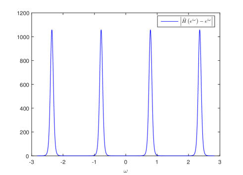
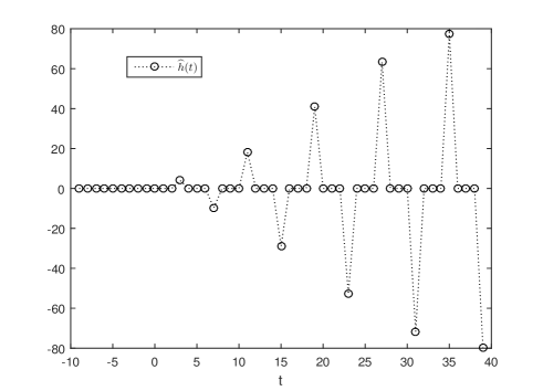
Figure 1: Approximation of the one-step forward shift operator: the values $|\widehat{H}\left(e^{i\omega}\right)-e^{i\omega}|$ for the transfer function of the predictor (4) and the values of the corresponding kernel $\widehat{h}={\cal Z}^{-1}\widehat{H}$ with $\gamma=4$, $r=0.4$, $m=4$.

Figure 1 shows an example of the shape of error curves for approximation of the forward one step shift operator. More precisely, they show the shape of $|\widehat{H}\left(e^{i\omega}\right)-e^{i\omega n}|$ for the transfer function (4) with $n=\nu=1$, and the shape of the corresponding predicting kernel $\widehat{h}$ with some selected parameters.

By the choice of $V$, it follows that $|V(z)|\to 0$ as $|z|\to+\infty$. Hence $v(0)=0$ for $v={\cal Z}^{-1}V$ and

$$V(z^{\nu m})=z^{-{\nu m}}v(1)+z^{-2{\nu m}}v(2)+z^{-3{\nu m}}v(3)+...$$

Clearly, we have that

$$V(z^{\nu m})^{n}=z^{-n{\nu m}}w(1)+z^{-(n+1){\nu m}}w(2)+z^{-(n+2){\nu m}}w(3)+...,$$

where $w={\cal Z}^{-1}(W)$ for $W(z)=V(z)^{n}$. Hence

$$\widehat{H}(z^{\nu m})=z^{n}V(z^{\nu m})^{n}=z^{n-n{\nu m}}w(1)+z^{n-(n+1){\nu m}}w(2)+z^{n-(n+2){\nu m}}w(3)+...$$

$$=z^{n-n{\nu m}}\widehat{h}(n{\nu m}-n)+z^{n-(n+1){\nu m}}\widehat{h}((n+1){\nu m}-n)+z^{n-(n+2){\nu m}}\widehat{h}((n+2){\nu m}-n)+...$$

In particular, $\widehat{H}\,\!\in{\rm H}^{\infty}(D^{c})$ and

$$\widehat{h}(k)=0\quad\hbox{if either}\quad(k+n)/m\notin{\mathbb{Z}}\quad\hbox{or}\quad k<mn-n.$$ (6)

(In fact, the sequence $\widehat{h}$ is more sparse for $n>1$ or $\nu>1$ than is shown in (6); nevertheless, (6) is sufficient for our purposes).

It can be noted that $\widehat{h}$ is real valued, since $\widehat{H}\,\!\left(\bar{z}\right)=\overline{\widehat{H}\,\!\left(z\right)}$.

Assume that we are given $x\in V(\delta,{\nu m})$. Let $X\stackrel{{\scriptstyle{\scriptscriptstyle\Delta}}}{{=}}{\cal Z}x$, $Y(z)=zX(z)$, and $\widehat{Y}\stackrel{{\scriptstyle{\scriptscriptstyle\Delta}}}{{=}}{\cal Z}\widehat{y}=\widehat{H}\,\!X$.

By the notations accepted above, it follows that $B_{1}$ is the unit ball in $\ell_{2}$. Let us show that

$$\sup_{k\in{\mathbb{Z}}}|x(k+n)-\widehat{y}(k)|\to 0\quad\hbox{as}\quad\gamma\to+\infty\quad\hbox{uniformly over}\quad x\in V(\delta,{\nu m})\cap B_{1},$$ (7)

where the process $\widehat{y}$ is the output of a linear predictor defined by the kernels $\widehat{h}$ as

$$\widehat{y}(k)\stackrel{{\scriptstyle{\scriptscriptstyle\Delta}}}{{=}}\sum^{k}_{p=-\infty}\widehat{h}(k-p)x(p).$$ (8)

This predictor produces the process $\widehat{y}(k)$ approximating $x(k+n)$ as $\gamma\to+\infty$ for all inputs $x\in V(\delta,{\nu m})$.

Remark 3

By (6),(8), an estimate $\widehat{y}(k)$ of $x(k+n)$ is constructed using the observations $\{x(k+n-qm)\}_{q\geq n,q\in{\mathbb{Z}}}$. This can be seen from representation of convolution (8) as

$$y(k)=\sum_{j\in{\mathbb{Z}},j\geq n}\widehat{h}(jm-n)x(k-jm+n).$$

Let $y(t)\stackrel{{\scriptstyle{\scriptscriptstyle\Delta}}}{{=}}x(t+n)$ and $Y={\cal Z}y$. We have that $\|Y\left(e^{i\omega}\right)-\widehat{Y}\left(e^{i\omega}\right)\|_{L_{1}(-\pi,\pi)}=I_{1}+I_{2},$ where

$$I_{1}=\int_{Q(\alpha)}|Y\left(e^{i\omega}\right)-\widehat{Y}\left(e^{i\omega}\right)|d\omega,\qquad I_{2}=\int_{Q_{+}(\alpha)}|Y\left(e^{i\omega}\right)-\widehat{Y}\left(e^{i\omega}\right)|d\omega.$$

By the definitions, there exists $\gamma_{0}>0$ such that, for all $\gamma>\gamma_{0}$, we have that

$$Q(\alpha)\subset J_{\delta,m},\quad I_{1}=0.$$ (9)

This means that $I_{1}\to 0$ as $\gamma\to+\infty$ uniformly over $x\in V(\delta,{\nu m})\cap B_{1}$.

Let us estimate $I_{2}$. We have that

$$I_{2}=\int_{Q_{+}(\alpha)}|(e^{i\omega n}-H\,\!\left(e^{i\omega}\right))X\left(e^{i\omega}\right)|d\omega\leq\int_{Q_{+}(\alpha)}|e^{i\omega n}(1-V\left(e^{i\omega{\nu m}}\right)^{n})X\left(e^{i\omega}\right)|d\omega$$

$$\leq\|1-V\left(e^{i\omega{\nu m}}\right)^{n}\|_{L_{2}(Q_{+}(\alpha))}\|X\left(e^{i\omega}\right)\|_{L_{2}(-\pi,\pi)}.$$

Further, ${\mathbb{I}}_{Q_{+}(\alpha)}(\omega)|1-V\left(e^{i\omega{\nu m}}\right)^{n}|\to 0$ a.e. as $\gamma\to+\infty$. By (5),

$${\mathbb{I}}_{Q_{+}(\alpha)}(\omega)|1-V\left(e^{i\omega{\nu m}}\right)^{n}|\leq 2^{n},\quad\forall\gamma:\ \gamma>\gamma_{0}.$$

From Lebesgue Dominance Theorem, it follows that $\|1-V\left(e^{i\omega{\nu m}}\right)^{n}\|_{L_{2}(Q_{+}(\alpha))}\to 0$ as $\gamma\to+\infty$. It follows that $I_{1}+I_{2}\to 0$ uniformly over $x\in V(\delta,{\nu m})\cap B_{1}$. Hence (7) holds and

$$\sup_{k\in{\mathbb{Z}}}|x(k+n)-\widehat{y}(k)|\to 0\quad\hbox{as}\quad\gamma\to+\infty\quad\hbox{uniformly over}\quad x\in V(\delta,{\nu m})\cap B_{1}.$$

Hence the predicting kernels $\widehat{h}={\cal Z}^{-1}\widehat{H}\,\!$ are such as required.

To complete the proof of Lemma 1, it suffices to prove that if $x$ is such that $x(k\varkappa+n)=0$ for $k\leq s$, then $x(k\varkappa+n)=0$ for $k>q$ for all $q\in{\mathbb{Z}}$. By the predictability established by (7) for a process $x\in V(\delta,{\nu m})$ such that $x(k\varkappa+n)=0$ for $k\leq s$, it follows that $x(k\varkappa+\varkappa+n)=0$; we obtain this by letting $\gamma\to+\infty$ in (4). (See also Remark 3). Similarly, we obtain that $x(k\varkappa+2\varkappa+q)=0$. Repeating this procedure $n$, we obtain that $x(k\varkappa+n)=0$ for all $k\in{\mathbb{Z}}$. This completes the proof of Lemma 1. $\Box$

Remark 4

Assume that $\{\widehat{x}_{d}\}_{d=-m+1}^{m-1}\in{\cal U}(\delta,m)$ for some $\delta>0$.

1. Lemma 1 applied with $\varkappa=1$ implies that all $\widehat{x}_{d}$ are uniquely defined by $\{\widehat{x}_{0}(k)\}_{k\in{\mathbb{Z}}^{-}}$ for $d=0,1,...,m-1$.

2. Lemma 1 applied with $\varkappa=m$ and $n=0$ implies that all values $\widehat{x}_{d}(mk)$ for $k>0$ are uniquely defined by the sequence $\{\widehat{x}_{0}(mk)\}_{k\in{\mathbb{Z}}^{+}}$ for $d=-m+1,1,...,1$.

Proof of Theorem 1. Let us prove statements (i)-(ii) for $s=0$. Let $d\in\{0,1,...,m-1\}$. By Lemma 1 applied with $\varkappa=m$, we have that a sequence $\{\widehat{x}_{d}(mk)\}_{k\geq 1}$ is uniquely defined by the sequence $\{\widehat{x}_{d}(mk)\}_{k\leq 0}$ (see Remark 3 above). Since $\{\widetilde{x}(mk-d)\}_{k\geq 1}=\{\widehat{x}_{d}(mk)\}_{k\geq 1}$ and $\{\widehat{x}_{d}(mk)\}_{k\leq 0}=\{\widetilde{x}(mk)\}_{k\leq 0}$, this implies that both sequences $\{\widetilde{x}(mk-d)\}_{k\geq 1}$ and $\{\widehat{x}_{d}(mk)\}_{k\geq 1}$ are uniquely defined by the sequence $\{\widetilde{x}(mk)\}_{k\leq 0}$. This completes statements (i) for the case where $s=0$.

Similar reasoning can be applied for statement (ii). Let $d\in\{-m+1,...,0\}$. By Lemma 1 applied with $\varkappa=m$ again, we have that a sequence $\{\widehat{x}_{d}(mk)\}_{k\leq-1}$ is uniquely defined by the sequence $\{\widehat{x}_{d}(mk)\}_{k\geq 0}$. Since $\{\widetilde{x}(mk-d)\}_{k\leq-1}=\{\widehat{x}_{d}(mk)\}_{k\leq-1}$ and $\{\widehat{x}_{d}(mk)\}_{k\geq 0}=\{\widetilde{x}(mk)\}_{k\geq 0}$, this implies that both sequences $\{\widetilde{x}(mk-d)\}_{k\leq-1}$ and $\{\widehat{x}_{d}(mk)\}_{k\leq-1}$ are uniquely defined by the sequence $\{\widetilde{x}(mk)\}_{k\geq 0}$. This completes statements (ii) for the case where $s=0$. Further, statements (i)-(ii) for $s\neq 0$ follows from the corresponding statements for $s=0$ applied for the sequences with shifted time $\{\widetilde{x}(k+s)\}$ and $\{\widehat{x}_{d}(k+s)\}$. Statements (i)-(ii) imply statement (iii). This completes the proof of Theorem 1. $\Box$

Proof for Example 1. It suffices to show that $s_{\mu(m,d_{1}),k}\neq s_{\mu(m,d_{2}),l}$ if $d_{1}\neq d_{2}$ for all $k,l\in{\mathbb{Z}}$. Suppose that $s_{\mu(m,d_{1}),k}=s_{\mu(m,d_{2}),l}$ for some $k,l\in{\mathbb{Z}}$ for $d_{2}=d_{1}+r$, for some $d_{1},d_{2}\in\{-m+1,...,m-1\}$ such that $r\stackrel{{\scriptstyle{\scriptscriptstyle\Delta}}}{{=}}d_{2}-d_{1}>0$. In this case, the definitions imply that

$$\frac{2k-1}{2^{d_{1}}}=\frac{2l-1}{2^{d_{2}}}.$$

This means that $2^{r}(2k-1)=2l-1$, and, therefore the number $2^{r}(2k-1)$ is odd. This is impossible since we had assumed that $r>0$. Hence the sets $J_{\delta,\mu(m,d)}$ are disjoint for different $d$ for small $\delta>0$. This completes the proof for Example 1. $\Box$

Proof of Theorem 2. Without a loss of generality, we assume that all $\delta$ used below are small enough to ensure that the sets $J_{\delta,\mu(m,d)}$ are disjoint for different $d$.

Let $Y_{d}\stackrel{{\scriptstyle{\scriptscriptstyle\Delta}}}{{=}}X_{0}-X_{d}$ and $y_{d}={\cal Z}^{-1}Y_{d}$, where $X_{d}={\cal Z}x_{d}$, $d=-m+1,...,m-1$. Since $x_{d}(k)=x_{0}(k)$ for $k\leq 0$ and $d>0$, and $x_{d}(k)=x_{0}(k)$ for $k\geq 0$ and $d<0$, it follows that $y_{d}(k)=0$ for $k\leq 0$ and $d>0$, and $y_{d}(k)=0$ for $k\geq 0$ and $d<0$. $d=1,2,...,m-1$. In addition, $Y_{0}\equiv 0$ and $y_{0}\equiv 0$.

Further, let ${\cal T}=\{k\in{\mathbb{Z}}:\ |k|\leq m-1,\ k\neq 0\}$, let

$$\widehat{X}_{0}\left(e^{i\omega}\right)\stackrel{{\scriptstyle{\scriptscriptstyle\Delta}}}{{=}}X_{0}\left(e^{i\omega}\right){\mathbb{I}}_{\{\omega\notin\cup_{d=-m+1}^{m-1}J_{\delta,\mu(m,d)}\}}+\sum_{d\in{\cal T}}Y_{d}\left(e^{i\omega}\right){\mathbb{I}}_{\{\omega\in J_{\delta,\mu(m,d)}\}},$$

and let $\widehat{X}_{d}\stackrel{{\scriptstyle{\scriptscriptstyle\Delta}}}{{=}}\widehat{X}_{0}-Y_{d}$ for $d\in{\cal T}$. By the definitions,

$$\widehat{X}_{d}\left(e^{i\omega}\right)=\widehat{X}_{0}\left(e^{i\omega}\right)-X_{0}\left(e^{i\omega}\right)+X_{d}\left(e^{i\omega}\right)=X_{d}\left(e^{i\omega}\right)+\sum_{p\in{\cal T}}(Y_{p}\left(e^{i\omega}\right)-X_{0}\left(e^{i\omega}\right)){\mathbb{I}}_{\{\omega\in J_{\delta,\mu(m,p)}\}}$$

$$=X_{d}\left(e^{i\omega}\right)-\sum_{p\in{\cal T}}X_{p}\left(e^{i\omega}\right){\mathbb{I}}_{\{\omega\in J_{\delta,\mu(m,p)}\}}$$

$$=X_{d}\left(e^{i\omega}\right){\mathbb{I}}_{\{\omega\notin J_{\delta,\mu(m,d)}\}}-\sum_{p\in{\cal T},p\neq d}X_{p}\left(e^{i\omega}\right){\mathbb{I}}_{\{\omega\in J_{\delta,\mu(m,p)}\}},\quad$$

$$d=-m+1,...,m-1.$$

Since the sets $J_{\delta,\mu(m,d)}$ are mutually disjoint, it follows that $\widehat{X}_{d}\left(e^{i\omega}\right)=0$ for $\omega\in J_{\delta,\mu(m,d)}$ and for all $d$. Hence $\widehat{x}_{d}\stackrel{{\scriptstyle{\scriptscriptstyle\Delta}}}{{=}}{\cal Z}^{-1}\widehat{X}_{d}\in V(\delta,\mu(m,d))$ for all $d$. It follows that the branching process $\{\widehat{x}_{d}\}_{d=-m+1}^{m-1}$ belongs to $\cup_{\delta>0}{\cal U}(\delta,m)$. In particular, $\widehat{x}_{d}(k)=\widehat{x}_{0}(k)$, for $k\leq 0$ and $d>0$, and $\widehat{x}_{d}(k)=\widehat{x}_{0}(k)$, for $k\geq 0$ and $d<0$. Clearly, $\|\widehat{x}_{d}-x_{d}\|_{\ell_{2}}\to 0$ as $\delta\to 0$ for $d=-m+1,,...,m-1$. This completes the proof of Theorem 2. $\Box$

Proof of Theorem 3. Let $\{x_{d}\}_{d=-m+1}^{m-1}$, $\{\widehat{x}_{d}\}_{d=-m+1}^{m-1}\in\cup_{\delta>0}{\cal U}(\delta,m)$ be such that suggested in the theorem’s statement. By the definitions, it follows that

$$\widetilde{x}(k)-x(k)=\widehat{x}_{d}(k+d)-x_{d}(k+d),\quad k\geq 0,\quad d\geq 0,\quad(k+d)/m\in{\mathbb{Z}},$$

and

$$\widetilde{x}(k)-x(k)=\widehat{x}_{d}(k+d)-x_{d}(k+d),\quad k<0,\quad d<0,\quad(k+d)/m\in{\mathbb{Z}}.$$

Then (3) follows from (2). This completes the proof of Theorem 3. $\Box$

Proof of Theorem 4. It suffices to show that the error for recovery a singe term $\widetilde{x}(n)$ for a given integer $n$ from the sequence $\{\widetilde{x}(mk)\}_{k\in{\mathbb{Z}},\,k\leq 0}$ can be made arbitrarily small is a well-posed problem; the proof for a finite set of values to recover is similar. Furthermore, it suffices to consider $n>0$; the case of $n<0$ can be considered similarly.

Let us consider an input sequence $x\in\ell_{2}$ such that

$$x=\widetilde{x}+\eta,$$ (10)

where $\eta\in\ell_{2}$ represents a noise, and where $\widetilde{x}\in U(\delta,m)$ is the representative branch for a branching process $\{\widehat{x}_{d}\}_{d=-m+1}^{m-1}\in{\cal U}(\delta,m)$.

Let $\eta_{n}\in\ell_{2}$ be defined such that $\eta_{n}(k)=\eta(k){\mathbb{I}}_{\{k\leq n\}}$. Let $N\stackrel{{\scriptstyle{\scriptscriptstyle\Delta}}}{{=}}{\cal Z}\eta_{n}$, and let $\sigma=\|N\left(e^{i\omega}\right)\|_{L_{2}(-\pi,\pi)}$; this parameter represents the intensity of the noise. Let $X={\cal Z}x$, $\widehat{X}_{d}={\cal Z}\widehat{x}_{d}$, and $N={\cal Z}\eta$.

Let $d\in\{0,1,...,m-1\}$ be such that $(n+d)/m\in{\mathbb{Z}}$.

Let $\delta>0$ be given and an arbitrarily small $\varepsilon>0$ be given. Assume that the parameters $(\gamma,r)$ of $V$ and $\widehat{H}$ in (4) are selected such that

$$\sup_{k\in{\mathbb{Z}}}|\bar{x}(k+n)-\bar{y}(k)|\leq\varepsilon/2\quad\forall\bar{x}\in V(\delta,\mu(m,d))\cap B_{1},$$ (11)

for $\bar{y}={\cal Z}^{-1}(\widehat{H}\bar{X})$ and $\bar{X}={\cal Z}\bar{x}$. Here $\widehat{H}$ is selected by (4), and $B_{1}$ is the unit ball in $\ell_{2}$.

By the choice of $d$, we have that there exists $p\in{\mathbb{Z}}$, $p\geq 1$, such that $n=pm-d$ and

$$\widehat{x}_{d}(pm)=\widetilde{x}(pm-d)=\widetilde{x}(n).$$ (12)

By (6) and Remark 3, the kernel $\widehat{h}$ produces an estimate $y_{d}$ of $\widehat{x}_{d}(pm)$ based on observations of $\{\widehat{x}_{d}(km)\}_{k<0}$.

Let us assume first that $\sigma=0$. In this case, we have that

$$\widehat{E}\stackrel{{\scriptstyle{\scriptscriptstyle\Delta}}}{{=}}|\widehat{y}_{d}(0)-\widehat{x}_{d}(pm)|=|\widehat{y}_{d}(0)-\widetilde{x}(n)|\leq\varepsilon/2.$$ (13)

Let us consider the case where $\sigma>0$. In this case, we have that

$$|\widehat{y}_{d}(0)-\widehat{x}_{d}(pm)|=|\widehat{y}_{d}(0)-x(n)|\leq\widehat{E}+E_{\eta},$$

where

$$E_{\eta}\stackrel{{\scriptstyle{\scriptscriptstyle\Delta}}}{{=}}\frac{1}{2\pi}\|(\widehat{H}\left(e^{i\omega}\right)-e^{i\omega n})N\left(e^{i\omega}\right)|\|_{L_{1}(-\pi,\pi)}\leq\sigma(\kappa+1),$$

and where

$$\kappa\stackrel{{\scriptstyle{\scriptscriptstyle\Delta}}}{{=}}\sup_{\omega\in[-\pi,\pi]}|\widehat{H}\left(e^{i\omega}\right)|.$$

Assume that $\eta(k)=\xi(k){\mathbb{I}}_{\{-N\leq k\leq n\}}-\widehat{x}_{0}(k){\mathbb{I}}_{\{k<-N\}}$, for an integer $N>0$. In this case, (10) gives that $x(k)=(x_{0}(k)+\xi(k)){\mathbb{I}}_{\{k>-N\}}$ for $k\leq n$. In addition, we have in this case that $\sigma\to 0$ as $N\to+\infty$ and $\|\xi\|_{\ell_{2}(-N,0)}\to 0$. If $N$ is large enough and $\|\xi\|_{\ell_{2}(-N,0)}$ is small enough such that $\sigma(\kappa+1)<\varepsilon/2$, then $\|\widehat{y}_{d}(0)-x(n)\|_{\ell_{\infty}}\leq\varepsilon$. This completes the proof of Theorem 4. $\Box$

Remark 5

By the properties of $\widehat{H}$, we have that $\kappa\to+\infty$ as $\gamma\to+\infty$. This implies that error (13) will be increasing if $\widehat{\varepsilon}\to 0$ for any given $\sigma>0$. This means that, in practice, the predictor should not target too small a size of the error, since in it impossible to ensure that $\sigma=0$ due inevitable data truncation.

Proof of Theorem 5. The previous proof shows that $\widetilde{x}\in\ell_{2}$. For $\widetilde{X}={\cal Z}\widetilde{x}$, we have that

$$\widetilde{x}(k)=\frac{1}{2\pi}\int_{-\pi}^{\pi}\widetilde{X}\left(e^{i\nu}\right)e^{i\nu k}d\nu=\frac{\tau}{2\pi}\int_{-\pi/\tau}^{\pi/\tau}\widetilde{X}\left(e^{i\tau\omega}\right)e^{i\omega\tau k}d\omega,$$

with the change of variables $\nu=\tau\omega$. Let us define function $\widetilde{F}:i{\bf R}\to{\bf C}$ as $\widetilde{F}(i\omega)\stackrel{{\scriptstyle{\scriptscriptstyle\Delta}}}{{=}}\tau\widetilde{X}\left(e^{i\tau\omega}\right)$ for $\omega\in{\bf R}$. Then

$$\widetilde{x}(k)=\frac{1}{2\pi}\int_{-\pi/\tau}^{\pi/\tau}\widetilde{F}\left(i\omega\right)e^{i\omega\tau k}d\omega.$$

Since $\widetilde{X}\left(e^{i\cdot}\right)\in L_{2}(-\pi,\pi)$, this implies that $\widetilde{F}\left(i\cdot\right)\in L_{2}(i{\bf R})$. The sequence $\{\widetilde{x}(k)\}_{k\in{\mathbb{Z}}}$ represents the sequence of Fourier coefficients of $\widetilde{F}$ and defines $\widetilde{F}$ uniquely. By Theorem 1, this sequence is uniquely defined by the sequence $\{\widetilde{x}(mk)\}_{k\in{\mathbb{Z}}}$. Let $\widetilde{f}\stackrel{{\scriptstyle{\scriptscriptstyle\Delta}}}{{=}}{\cal F}\widetilde{F}$. Clearly, $\widetilde{f}\in L_{2}^{{\scriptscriptstyle BL},\pi/\tau}({\bf R})$ and it is uniquely defined by the sequence $\{\widetilde{x}(mk)\}_{k\in{\mathbb{Z}}}$. This completes the proof of Theorem 5. $\Box$

Proof of Corollary 1. We use notations from the proofs above. The existences of the required $\{\widehat{x}_{d}\}_{-m+1}^{m-1}$, $\widetilde{x}$, and $\widetilde{f}$, follows from Theorem 1-2. We have for $F={\cal F}f$ that, for some $\bar{C}>0$, that

$$\|\widetilde{F}(i\cdot)-F(i\cdot)\|_{L_{2}({\bf R})}=\sqrt{\tau}\|\widetilde{x}-x\|_{\ell_{2}}\leq\sqrt{\tau}\sum_{d=-m+1}^{m-1}\|\widehat{x}_{d}-x_{d}\|_{\ell_{2}}\leq\sqrt{\tau}(2m-1)\varepsilon.$$

Since $F(i\omega)=0$ and $\widetilde{F}(i\omega)=0$ if $|\omega|>\pi/\tau$, it follows that

$$\|\widetilde{F}(i\cdot)-F(i\cdot)\|_{L_{1}({\bf R})}\leq\sqrt{2\Omega}\|\widetilde{F}(i\cdot)-F(i\cdot)\|_{L_{2}({\bf R})}.$$

Combining these estimates, we obtain that

$$\|\widetilde{f}-f\|_{L_{p}({\bf R})}\leq 2\pi\max(1,\sqrt{2\Omega})\|\widetilde{F}(i\cdot)-F(i\cdot)\|_{L_{2}({\bf R})}\leq 2\pi\max(1,\sqrt{2\Omega})\sqrt{\tau}(2m-1)\varepsilon.$$

This completes the proof of Corollary 1. $\Box$

Proof of Corollary 2. It suffices to observe that $\widetilde{x}(k)=\widetilde{f}(t_{k})$ satisfy the assumptions of of Corollary 2. $\Box$

Proof of Corollary 3. We have that

$$\sup_{t\in{\bf R}}|f(t)-f_{\Omega}(t)|\leq\frac{1}{2\pi}\int_{-\infty}^{\infty}|F(i\omega)-F_{\Omega}(i\omega)|d\omega=\frac{1}{2\pi}\int_{{\bf R}\setminus[-\Omega,\Omega]}|F(i\omega)|d\omega\to 0\quad$$

$$\hbox{as}\quad\Omega\to+\infty,\ m\to+\infty.$$

Then statement (i) follows. The function $f_{\Omega}$ has the same properties as the function $f$ in Corollary 1. This completes the proof of Corollary 3. $\Box$

5 Discussion and future developments

The paper shows that recoverability of sequences from their decimated subsequences is associated with certain spectrum degeneracy of a new kind, and that a sequences of a general kind can be approximated by sequences featuring this degeneracy. This is applied to sparse sampling of continuous time band-limited functions. The paper suggests a uniqueness result for sparse sampling (Theorems 3 and Theorem 1), and establishes some robustness of recovery (Theorems 4 and Theorem 2). This means that the restriction on the sampling rate defined by the Nyquist rate the Sampling Theorem is bypassed, in a certain sense. This was only the very first step in attacking the problem; the numerical implementation to data compression and recovery is quite challenging and there are many open questions. In particular, it involves the solution of ill-posed inverse problems. In addition, there are other possible extensions of this work that we will leave for the future research.

1. A theoretical problem arises: How to detect a trace $x_{0}|_{k\leq 0}$ that can be extended into a branching process featuring degeneracy described in Definition 3 for $d>0$? This is actually a non-trivial question even for $m=1$; see discussion Definition 1 in [6] and discussion in [5, 6, 8].

2. To cover applications related to image processing, the approach of this paper has to be extended on 2D sequences and functions $f:{\bf R}^{2}\to{\bf R}$. This seems to be a quite difficult task; for instance, our approach is based on the predicting algorithm [3] for 1D sequences, and it is unclear if it can be extended on processes defined on multidimensional lattices. Possibly, the setting from PM [18] can be used.

3. The result of this paper allows many acceptable modifications such as the following.

   – The choice of mappings ${\cal M}_{d}$ allows many modifications; for example, $x_{d}={\cal M}_{d}x$ are defined such that there exists $\theta\geq m$ such that $x_{d}(k)=x(k-d)$ for $k>\theta$, without any restrictions on $\{x_{d}(k)\}_{k=1,..,\theta}$.

   – Conditions of Theorem 1 can be relaxed: instead of the condition that the spectrum vanishes on open sets $J_{\delta,m}$, we can require that the spectrum vanishes only at the middle points of the intervals forming $J_{\delta,m}$; however, the rate of vanishing has to be sufficient, similarly to D12a [3]. This is because the predicting algorithm D12a [3] does not require that the spectrum of an underlying process is vanishing on an open subset of ${\mathbb{T}}$.

   – The choice (4) of predictors presented in the proofs above is not unique. For example, we could use a predicting algorithm from Dokuchaev [4] instead of the the algorithm based on D12a [3] used above. Some examples of numerical experiments for the predicting algorithm based on the transfer function (4) can be found in Dokuchaev [7] (for the case where $m=n=1$, in the notations of the present papers).

Acknowledgment

This work was supported by ARC grant of Australia DP120100928 to the author.

References

• [1] Beurling, A., Malliavin, P. (1967). On the closure of characters and the zeros of entire functions, Acta Mathematica 118 79–93.
• Cai [2009] T. Cai, G. Xu, and J. Zhang. (2009), On recovery of sparse signals via $\ell_{1}$ minimization, IEEE Trans. Inf. Theory, vol. 55, no. 7, pp. 3388-3397.
• [3] Dokuchaev, N. (2012). Predictors for discrete time processes with energy decay on higher frequencies. IEEE Transactions on Signal Processing 60, No. 11, 6027-6030.
• Dokuchaev [2012] Dokuchaev, N. (2012). On predictors for band-limited and high-frequency time series. Signal Processing 92, iss. 10, 2571-2575.
• [5] Dokuchaev, N. (2012). Causal band-limited approximation and forecasting for discrete time processes. ArXiv 1208.3278.
• [6] Dokuchaev, N. (2016). On recovering missing values in a pathwise setting. ArXiv: https://arxiv.org/abs/1604.04967.
• Dokuchaev [2016] Dokuchaev, N. (2016). Near-ideal causal smoothing filters for the real sequences. Signal Processing 118, iss. 1, pp. 285-293.
• [8] Dokuchaev, N. (2017). On detecting predictability of one-sided sequences. Digital Signal Processing 62 26-29.
• [9] Ferreira P. G. S. G.. (1992). Incomplete sampling series and the recovery of missing samples from oversampled bandlimited signals. IEEE Trans. Signal Processing 40, iss. 1, 225-227.
• [10] Ferreira P. G. S. G.. (1995). Sampling Series With An Infinite Number Of Unknown Samples. In: SampTA’95, 1995 Workshop on Sampling Theory and Applications, 268-271.
• Jerri [1977] Jerri, A. (1977). The Shannon sampling theorem - its various extensions and applications: A tutorial review. Proc. IEEE 65, 11, 1565–1596.
• [12] Kotelnikov, V.A. (1933). On the carrying capacity of the ether and wire in telecommunications. Material for the First All-Union Conference on Questions of Communication, Izd. Red. Upr. Svyazi RKKA, Moscow, 1933.
• [13] Landau H.J. (1964). A sparse regular sequence of exponentials closed on large sets. Bull. Amer. Math. Soc. 70, 566-569.
• [14] Landau H.J. (1967). Sampling, data transmission, and the Nyquist rate. Proc. IEEE 55 (10), 1701-1706.
• [15] Nyquist, H. (1928). Certain topics in telegraph transmission theory, Trans. AIEE, Trans., vol. 47, pp. 617–644.
• [16] Olevski, A., and Ulanovskii, A. (2008). Universal sampling and interpolation of band-limited signals. Geometric and Functional Analysis, vol. 18, no. 3, pp. 1029–1052.
• [17] Olevskii A.M. and Ulanovskii A. (2016). Functions with Disconnected Spectrum: Sampling, Interpolation, Translates. Amer. Math. Soc., Univ. Lect. Ser. Vol. 46.
• [18] Petersen, D.P. and Middleton D. (1962). Sampling and reconstruction of wave-number-limited functions in N-dimensional Euclidean spaces. Information and Control, vol. 5, pp. 279–323.
• [19] Shannon, C.E. (1949). Communications in the presence of noise, Proc. Institute of Radio Engineers, vol. 37, no.1, pp. 10 21.
• [20] Ulanovskii, A. (2001). On Landau’s phenomenon in $R^{n}$. Mathematica Scandinavica, vol. 88, no. 1, 72–78.
• [21] Ulanovskii, A. (2001). Sparse systems of functions closed on large sets in $R^{N}$, Journal of the London Mathematical Society, vol. 63, no. 2, 428–440.
• [22] Unser, M. (2000). Sampling 50 years after Shannon, Proceedings of the IEEE, vol. 88, pp. 569–587.
• [23] Vaidyanathan P. P. (1987). On predicting a band-limited signal based on past sample values, in Proceedings of the IEEE, vol. 75, no. 8, pp. 1125-1127.
• [24] Vaidyanathan, P.P. (2001). Generalizations of the Sampling Theorem: Seven Decades After Nyquist. IEEE Transactions on circuits and systems I: fundamental theory and applications, v. 48, NO. 9,
• [25] Whittaker, E.T. (1915). On the Functions Which are Represented by the Expansions of the Interpolation Theory. Proc. Royal Soc. Edinburgh, Sec. A, vol.35, pp. 181 194.
• Yosida [1965] Yosida, K. (1965). Functional Analysis. Springer, Berlin Heilderberg New York.
• [27] Zayed A. (1993). Advances in Shannon’s Sampling Theory. Boca Raton, CRC Press, N.Y, London, Tokyo.
Refer to caption
Refer to caption