Hybrid Spectrum Access for mmWave Networks

Abstract

While spectrum at millimeter wave (mmWave) frequencies is less scarce than at traditional frequencies below 6 GHz, still it is not unlimited, in particular if we consider the requirements from other services using the same band and the need to license mmWave bands to multiple mobile operators. Therefore, an efficient spectrum access scheme is critical to harvest the maximum benefit from emerging mmWave technologies. In this paper, motivated by previous results where spectrum pooling was proved to be more feasible at high mmWave frequencies, we study the performance of a hybrid spectrum scheme where exclusive access is used at frequencies in the 20/30 GHz range while spectrum pooling/unlicensed spectrum is used at frequencies around 70 GHz. Our preliminary results show that hybrid spectrum access is a promising approach for mmWave networks, and motivate further studies to achieve a more complete understanding of both technical and non technical implications.

I Introduction

The potential of orders of magnitude increases in capacity offered by the millimeter wave (mmWave) frequencies poses new spectrum access challenges. In this paper, we introduce a hybrid scheme that builds on both exclusive access and spectrum pooling concepts.

Traditionally, wireless data services have been delivered mainly by using two different spectrum access models. Under the exclusive model, each mobile operator is granted the right of exclusive use of a spectrum band to provide mobile services. Exclusive spectrum access has been one of the key factors for the successful deployment of cellular systems since their inception, and it is by far the default model to provide mobile services. Under the license-exempt (also referred to as unlicensed) model, spectrum is allowed to be used by several users/mobile operators. While there is no guaranteed access to an instantaneously fixed amount of spectrum, politeness rules (e.g., based on a listen-before-talk principle) are in place to allow a fair use of the spectrum. The license-exempt spectrum model has been one of the key factors for the successful deployment of WiFi as a ubiquitous way of connecting devices to the Internet. The spectrum pooling model has also been considered as an intermediate paradigm, where different operators are granted access to the same spectrum resources, with rules that are known a priori. Spectrum pooling does not provide guarantees for the access to an instantaneously fixed amount spectrum, but ensures some level of predictability and short-term and long-term fairness [1].

Recently, new technologies emerged that aggregate spectrum in both exclusive and license-exempt bands, in a way to route the different information pipes to the carrier that best matches their requirements. Aggregation can be implemented at the MAC layer, to allow a very rapid switch between exclusive and license-exempt carriers, effectively realising a hybrid spectrum access regime. Examples of these technologies are Licensed Assisted Access (LAA), LTE-WiFi link aggregation and LTE-WiFi interworking. We note that hybrid spectrum access has been proposed for traditional spectrum below 6 GHz as an extension of carrier aggregation, while to the best of our knowledge there are no works assessing the benefit of hybrid spectrum access for mmWave networks.

While spectrum at mmWave frequencies is less scarce than at traditional frequencies below 6 GHz, still it is not unlimited, in particular if we consider the requirements from other services (e.g., satellite and fixed services) and the need to license mmWave bands to multiple mobile operators. Therefore, an efficient spectrum access scheme is critical to harvest the maximum benefit from emerging mmWave technologies  [2]. Recent works compared exclusive spectrum allocation with different types of spectrum pooling or unlicensed models, showing different results as a function of the assumptions used. Reference [3] introduced a new signaling report among mobile operators, to establish an interference database to support scheduling decisions, with both a centralized and a distributed supporting architecture. In the centralized case, a new architectural entity receives information about the interference measured by each network and determines which links cannot be scheduled simultaneously. In the decentralized case, the victim network sends a message to the interfering network with a proposed coordination pattern. The two networks can further refine the coordination pattern via multiple stages. Reference [4] studied the feasibility of spectrum pooling in mmWave networks under the assumption of ideal antenna patterns and showed that spectrum pooling might be beneficial even without any coordination between the different operators. In particular, [4] showed that uncoordinated pooling provides gain at both 28 GHz and 73 GHz. Reference [2] further developed the results in [3] and [4], focusing on the effect of coordination and of inaccurate beamforming. It showed that, while coordination may not be needed under ideal assumptions, it does provide substantial gains when considering more realistic channel and interference models and antenna patterns. Moreover, it showed that, under realistic assumptions, spectrum pooling without coordination might be more feasible at high mmWave frequencies (e.g., 70 GHz) than at low mmWave frequencies (e.g., 28 or 32 GHz), due to the higher directionality of the beams. Reference [5] compares different resource sharing paradigms and shows that a full spectrum and infrastructure sharing configuration provides significant advantages, even without resorting to complex signaling protocols for the exchange of information between multiple operators’ networks.

This paper extends the previous results in [2] and [5] to the case of hybrid spectrum allocation. In other words, differently from the previous works, where exclusive access and spectrum pooling were compared, in this work we propose a spectrum access paradigm that builds on both exclusive access and unlicensed access/spectrum pooling. In particular, motivated by the results in [2] where pooling was proved to be more feasible at high mmWave frequencies, we study the performance of a hybrid spectrum scheme where exclusive access is used at frequencies in the 20/30 GHz range while pooling is used at frequencies around 70 GHz. The two bands are aggregated at the MAC layer as in Figure 1, and users are allocated to one or the other band to maximize the rate. In this way, interference-limited users are allocated to the exclusive spectrum component while noise-limited users are allocated to the pooled spectrum components. We compare our proposal with two baselines, one relying on exclusive spectrum access at both 28 GHz and 73 GHz and thus favoring interference-limited scenarios, the other relying on pooling at both 28 GHz and 73 GHz and thus favoring noise-limited scenarios. Our preliminary results show that hybrid spectrum access is a promising approach for mmWave networks, and motivate further studies for a more complete understanding of both technical and non technical implications.

The rest of the paper is organized as follows. In Section II, we describe the system model. In Section III, we describe the proposed hybrid spectrum allocation algorithm. In Section IV, we provide a numerical evaluation and discuss the results. Finally, we conclude the paper and describe some future research steps in Section V.

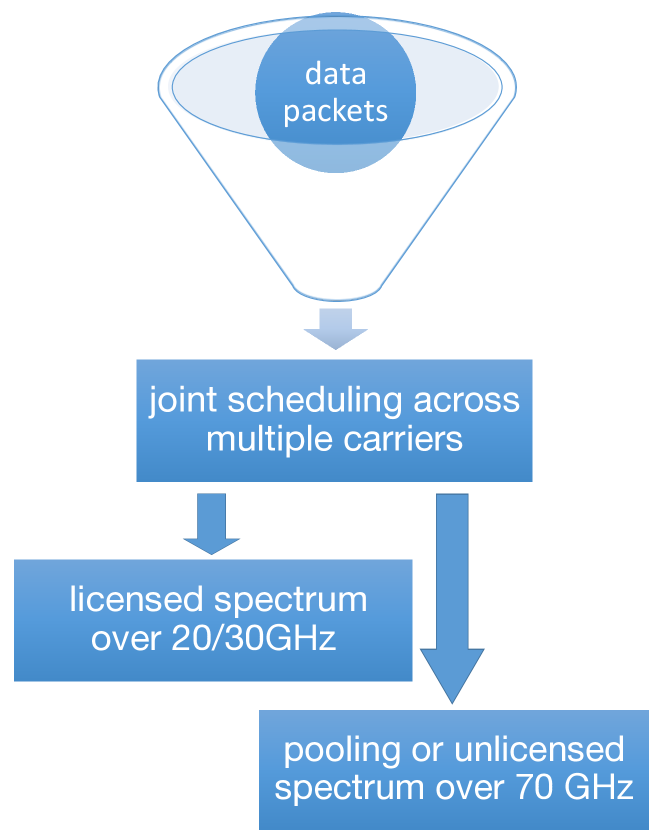
Figure 1: Blocks diagram of the joint scheduling that allocates user packets over the different bands.

II System model

We consider a scenario with $M$ operators, each with a set $\mathcal{I}_{m}$ of base stations (BSs) and a set $\mathcal{J}_{m}$ of user equipments (UEs). For each operator, both UEs and BSs are placed following a Poisson point process (PPP) with densities $\lambda_{\text{UE}}$ and $\lambda_{\text{BS}}$, respectively, which represents an unplanned deployment, where base stations are not optimally located. Moreover, we assume that all BSs support two mmWave bands, one at 28 GHz and one at 73 GHz. We assume a downlink transmission where for a given operator $m\in\{1,\ldots,M\}$ we define $\mathbf{x}_{mij}$ as the $n_{\text{TX}}\times 1$ transmitted vector between BS $i\in\{1,\ldots,I_{m}\}$ and UE $j\in\{1,\ldots,J_{m}\}$:

$$\mathbf{x}_{mij}=\mathbf{w}_{{\text{TX}}_{mij}}u_{mij},$$ (1)

where $n_{\text{TX}}$ is the number of antennas at the BS transmitter, $\mathbf{w}_{{\text{TX}}_{mij}}$ is the $n_{\text{TX}}\times 1$ beamforming vector between the $i$-th BS and the $j$-th UE of the $m$-th operator, and $u_{mij}$ is the corresponding scalar information symbol transmitted. We model the transmit antennas as a uniform planar array (UPA) at both BS and UE, and allow more antenna elements to be deployed at 73 GHz compared to 28 GHz. In particular, we assume that the numbers of antennas at the BS transmitter and at the UE receiver are $n_{\text{TX}}=64$ and $n_{\text{RX}}=16$ for the 28 GHz links, and $n_{\text{TX}}=256$ and $n_{\text{RX}}=64$ for the 73 GHz links. The beamforming gain from BS $i$ to UE $j$ of operator $m$ is given by:

$$G_{mij}=|\textbf{w}^{T}_{\text{RX}_{mij}}\textbf{H}_{mij}\textbf{w}_{\text{TX}_{mij}}|^{2},$$ (2)

where $\textbf{w}_{\text{TX}_{mij}}\in\mathbb{C}^{n_{\text{TX}}}$ is the beamforming vector of transmitter $i$ when transmitting to receiver $j$, $\textbf{w}_{\text{RX}_{mij}}\in\mathbb{C}^{n_{\text{RX}}}$ is the beamforming vector of receiver $j$ when receiving from transmitter $i$, and $\textbf{H}_{mij}$ is the channel matrix (described in the following). Beamforming vectors are computed as follow:

$$\textbf{w}(\Omega)=\frac{1}{\sqrt{n}}\begin{bmatrix}1\\ \exp(-j2\pi\Delta\Omega)\\ \exp(-j2\pi 2\Delta\Omega)\\ \vdots\\ \exp(-j2\pi(n-1)\Delta\Omega)\end{bmatrix},$$ (3)

where $\Delta$ represents the spacing between the elements of the array, $\Omega$ is the direction of transmission or reception (considering both horizontal and vertical angles), and $n$ is the normalization factor and corresponds to the number of elements in the antenna array. We assume to have the possibility of steering in any direction. Therefore, we can generate a beamforming vector for any possible angle between 0 and 360 degrees. We also assume perfect alignment between the beams of each UE and its serving BS. We consider the following transmit power constraint:

$$E\left[|u_{mij}^{*}u_{mij}|^{2}\right]\leq P,$$ (4)

where $P$ is the maximum power allowed at the input of the antenna array (or equivalently at the output of the power amplifier driving the antenna array). The received signal at the $i$-th user of the $m$-th operator is modeled as follows:

$$\textbf{y}_{mij}=\textbf{H}_{mij}\textbf{x}_{mij}+\textbf{n}_{mij},$$ (5)

where $\textbf{H}_{mij}$ is the channel matrix, modeled as composed of a random number $K$ of clusters, each corresponding to a macro-level scattering path, and $\textbf{n}_{mij}$ is the additive noise (which also includes interference). At the receiver, the number of clusters is given as the maximum between 1 and a Poisson random variable whose mean $\lambda$ is related to the carrier frequency as explained in [6]. For each cluster $k$, the number of sub-paths is modeled as an integer random variable uniformly distributed in $\{1,\ldots,10\}$. Given a set of clusters and of sub-paths for a channel, we can compute the channel matrix as:

$$\textbf{H}(t,f)=\sum_{k=1}^{K}\sum_{\ell=1}^{L_{k}}g_{k\ell}(t,f)\textbf{u}_{\text{RX}}(\theta^{\text{RX}}_{k\ell},\phi^{\text{RX}}_{k\ell})\textbf{u}^{*}_{\text{TX}}(\theta^{\text{TX}}_{k\ell},\phi^{\text{TX}}_{k\ell}),$$ (6)

where $L_{k}$ is the number of sub-paths in cluster $k$, $g_{k\ell}(t,f)$ is the small-scale fading of path $\ell$ in cluster $k$ over time and frequency, and $\textbf{u}_{\text{RX}}(\cdot)$ and $\textbf{u}_{\text{TX}}(\cdot)$ are the spatial signature vectors of the receiver and the transmitter, respectively. Spatial signatures are computed with horizontal and vertical angles of arrival (AoA) $\theta^{\text{RX}}_{k\ell},\phi^{\text{RX}}_{k\ell}$, and horizontal and vertical angles of departure (AoD) $\theta^{\text{TX}}_{k\ell},\phi^{\text{TX}}_{k\ell}$, where $k=1,\dots,K$ is the cluster index and $\ell=1,\dots,L_{k}$ is the sub-path index within the cluster. The small-scale fading (obtained from [6]) is generated based on the number of clusters, the number of sub-paths in each cluster, the Doppler shift, the power spread, and the delay spread, as:

$$g_{k\ell}(t,f)=\sqrt{P_{k\ell}}e^{j2\pi f_{d}cos(\omega_{k\ell})t}e^{-j2\pi\tau_{k\ell}f},$$ (7)

where $P_{k\ell}$ is the power spread of sub-path $\ell$ in cluster $k$, $f_{d}$ is the maximum Doppler shift, $\omega_{k\ell}$ is the angle of arrival of sub-path $\ell$ in cluster $k$ with respect to the direction of motion, $\tau_{k\ell}$ is the delay spread of sub-path $\ell$ in cluster $k$, and $f$ is the carrier frequency.

The power spread $P_{k\ell}$ is obtained by following [11]:

$$P_{k\ell}=\frac{P_{k\ell}^{\prime}}{\sum_{h=1}^{K}\sum_{p=1}^{L_{h}}P_{hp}^{\prime}},\quad P_{k\ell}^{\prime}=\frac{U_{k}^{r_{\tau}-1}10^{-0.1Z_{k}+V_{k\ell}}}{L_{k}},$$ (8)

where $U_{k}\sim U[0,1]$, $V_{k\ell}\sim U[0,0.6]$ and $Z_{k}\sim N(0,\zeta^{2})$, while parameters $r_{\tau}$ and $\zeta$ are found in [6].

Following the measurement campaign carried out in a real dense urban environment and reported in [7, 8, 9, 10], pathloss can be modeled with three states: line-of-sight (LoS), non-line-of-sight (NLoS) and outage. Each link is characterized by the channel state probabilities $p_{\mathrm{LoS}}$, $p_{\mathrm{NLoS}}$ and $p_{\mathrm{out}}$, which are expressed in terms of the distance $d$ between UE and BS as follows:

$$\begin{matrix}\vspace{-0.3cm}p_{\mathrm{out}}(d)=\mathrm{max}(0,1-e^{-a_{\mathrm{out}}d+b_{\mathrm{out}}})\\ \vspace{-0.3cm}p_{\mathrm{LoS}}(d)=(1-p_{\mathrm{out}}(d))e^{-a_{\mathrm{LoS}}d}\\ p_{\mathrm{NLoS}}(d)=1-p_{\mathrm{out}}(d)-p_{\mathrm{LoS}}(d),\end{matrix}$$ (9)

where $a_{\mathrm{out}}=0.0334$ m^-1, $b_{\mathrm{out}}=5.2$ and $a_{\mathrm{LoS}}=0.0149$ m^-1 (all these values are taken from [6]). The long-term pathloss, which includes distance dependent attenuation and log-normal shadowing, is then given by:

$$PL(d)[dB]=\alpha+\beta 10\log_{10}(d)+\xi,$$ (10)

where $\xi\sim N(0,\sigma^{2})$ is the log-normal shadowing, and parameters $\alpha,\beta,\sigma$ are reported in [6] for both the 28 and the 73 GHz bands, and for both LoS and NLoS.

III Hybrid UE association

Simulations are run in an area $A$ where users and base stations are placed following a PPP deployment for each mobile network $m\in\mathcal{M}$. In the primary phase of the algorithm, each UE $j\in\mathcal{J}_{m}$ in the area is associated to the BS $i\in\mathcal{I}_{m}$ that provides the minimum pathloss. More precisely, the pathloss is computed under the same state condition in both bands. In practice this means that if the link between a UE and a BS is in one of the three states (LoS, NLoS or outage), this state will be the same for both the 28 and 73 GHz bands. After the selection of the best BS, we randomly associate the UE to the BS band at 28 or 73 GHz, according to the probabilities $P_{28}$ and $P_{73}=1-P_{28}$. In this study, these probabilities are taken equal to $\tfrac{1}{2}$ (we have verified by simulation that in most cases users are roughly equally split between the two bands).

In the second and last step, we associate a reference UE $j^{*}$, located at the center of the area, to the BS $i^{*}$ and carrier $c^{*}$ that maximize the throughput. The optimization problem can be formulated as follows:

$$\left(c^{*},i^{*}\right)=\operatorname*{arg\,max}_{i\in\mathcal{I}_{m},c\in\mathcal{C}}\left(\frac{BW^{(c)}}{1+N^{(c)}_{mi}}\log_{2}\left(1+\gamma_{mij^{*}}^{(c)}\right)\right),$$ (11)

where $N_{mi}^{(c)}$ is the number of users already associated to the $c$-th carrier of the $i$-th base station and $BW^{(c)}$ is the bandwidth of the $c$-th carrier, $c\in\mathcal{C}=\{28\leavevmode\nobreak\ \text{GHz},73\leavevmode\nobreak\ \text{GHz}\}$. Then, we define the Signal-to-Interference-plus-Noise Ratio (SINR) term $\gamma_{mij^{*}}^{(c)}$ that considers the instantaneous interference value for UE $j^{*}$ allocated to the $c$-th carrier of the $i$-th BS, as:

$$\gamma_{mij^{*}}^{(c)}=\frac{\frac{P^{(c)}_{\text{TX}_{mi}}}{PL_{mij^{*}}^{(c)}}G^{(c)}_{mij^{*}}}{\sum_{k\neq i}\frac{P^{(c)}_{\text{TX}_{mk}}}{PL^{(c)}_{mkj^{*}}}G^{(c)}_{mkj^{*}}+BW^{(c)}N_{0}},$$ (12)

where $P^{(c)}_{\text{TX}_{mi}}$ denotes the transmit power, $G^{(c)}_{mij^{*}}$ denotes the antenna gain at the $c$-th carrier (computed in the following), $k$ represents each interfering link, $G_{mkj^{*}}^{(c)}$ is the antenna gain between BS ${k\neq i}$ and UE $j^{*}$, and $N_{0}$ is the thermal noise. Then, $PL_{mij^{*}}^{(c)}$ denotes the pathloss between UE $j^{*}$ and the $c$-th carrier of the $i$-th BS. We assume a perfect alignment between the BS and UE beams so as to achieve the maximum beamforming gain $G\,[\text{dB}]=10\log_{10}(n_{\text{TX}}n_{\text{RX}})$. Under the assumption of perfect alignment between BS and UE beams, the antenna gain of the intended link is only a function of the carrier used (i.e., at 73 GHz there is a higher gain than at 28 GHz thanks to the higher number of antennas). Therefore, the maximum beamforming gains $G^{(c)}_{mij^{*}}$ along the aligned directions, at 28 GHz and 73 GHz, are:

$$\centering\begin{split}G^{(28\,\text{GHz})}&=10\log_{10}(64\cdot 16)\simeq 30\,\text{dB}\\ G^{(73\,\text{GHz})}&=10\log_{10}(265\cdot 64)\simeq 42\,\text{dB}.\end{split}\@add@centering$$ (13)

It is important to highlight that $G^{(c)}_{mij^{*}}$ is computed as in Equation (2), where the actual antenna gain will be affected by the instantaneous channel fading. In a different manner, we note that the antenna gain $G_{mkj^{*}}^{(c)}$ between BS ${k\neq i}$ and UE $j^{*}$ is calculated assuming there is no alignment between transmit and receive beams, thus following Equation (2) with a realistic pattern and angle that depends on the relative positions of UE $j^{*}$ and interfering BS $k$ for operator $m$. In other words, we assume beam alignment for the link between a UE and its serving BS, while we do not assume beam alignment between a UE and an interfering BS.

Using the instantaneous SINR in (12), we can derive the throughput of the reference user $j^{*}$ as:

$$\eta_{mj^{*}}=\frac{BW^{(c^{*})}}{1+N_{mi^{*}}^{(c^{*})}}\log_{2}\left(1+\gamma_{mi^{*}j^{*}}^{(c^{*})}\right).$$ (14)

Repeating this two-step procedure a sufficient number of times (10⁴ in our results), we are able to capture the statistics of interest for the reference user and to evaluate the performance of the hybrid association procedure.

We summarize the proposed hybrid UE association procedure in Algorithm 1.

Algorithm 1

1:$\forall m\in\mathcal{M}$ deploy in the area $A$ $J_{m}$ UEs and $I_{m}$ BSs following a PPP;

2:for $\forall$ operator $m\in\mathcal{M}$ do

3:     for $\forall$ user $j\in\mathcal{J}_{m}$ do

4:         for $\forall$ BS $i\in\mathcal{I}_{m}$ do

5:              $PL_{mij}\leftarrow$ compute pathloss $\forall$ link $(i,j)$;

6:         end for

7:     end for

8:end for

9:$N$: matrix initialized to zeros used to count # UEs $\forall i\in\mathcal{I}_{m}$ and $\forall c\in\mathcal{C}$;

10:$\overline{M}$: vector that stores for each UE the $index$ of the associated BS;

11:for $\forall$ user $j\in\mathcal{J}_{m}$ and $\forall m\in\mathcal{M}$ do

12:     Associate user $j$ to the BS $i^{*}$ with minimum $PL_{mij}$;

13:     $p\leftarrow$ randomly pick a value $\in[0,1]$;

14:     if $p<0.5$ then

15:         $c^{*}\leftarrow$ 28 GHz band;

16:     else

17:         $c^{*}\leftarrow$ 73 GHz band;

18:     end if

19:     $N(i^{*},c^{*})\leftarrow N(i^{*},c^{*})+1$;

20:     $\overline{M}(j)\leftarrow i^{*}$;

21:end for

22:$P_{\text{TX}_{ic}}$: set equal to 30 dBm $\forall i\in\mathcal{I}_{m}$ and $\forall c\in\mathcal{C}$;

23:$G_{c}$: computed following Equations (13) $\forall c\in\mathcal{C}$;

24:$BW_{c}$: bandwidth set $\forall c\in\mathcal{C}$;

25:for $\forall$ BS $i\in\mathcal{I}_{m}$ do

26:     $\overline{\gamma}_{mij^{*}}^{(c)}\leftarrow$ compute matrix of SINRs $\forall i\in\mathcal{I}_{m}$, $\forall c\in\mathcal{C}$ as in (12);

27:     $\eta_{mj^{*}}\leftarrow$ compute matrix of rates using $\overline{\gamma}_{mij^{*}}^{(c)}$, $BW_{c}$, and $N(i,c)$;

28:     $\left(c^{*},i^{*}\right)\leftarrow\operatorname*{arg\,max}_{i\in\mathcal{I}_{m},c\in\mathcal{C}}{(\eta_{mj^{*}})}$;

29:end for

We note that:

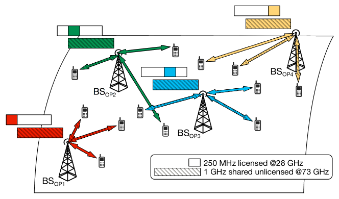
Figure 2: Hybrid spectrum access scheme. The 1 GHz band at 28 GHz is split among the four operators (exclusive spectrum access), while at 73 GHz the entire band of 1 GHz is shared among the operators (pooling).

• The approach in (11) maximizes the throughput of the reference UE after association of all the previous users according to a minimum pathloss criterion and to a random decision for the carrier. Therefore, this procedure leads to a suboptimal result. However, due to the large number of BSs and UEs in the system, we believe this proposal provides a good starting point to analyze the performance of hybrid spectrum allocation. We plan to study the gap with respect to the optimal allocation in our future work.

• The objective function in (11) considers the UE throughput. Another possible approach would be to consider the aggregate throughput within each BS or the total throughput in the system. We plan to explore these different approaches in our future work.

• We are currently assuming that the allocation algorithm is implemented in a centralized way. However, the algorithm could be implemented in a distributed way, assuming that a supporting signaling between BS and UE and inter-operator interference estimation capabilities at the UEs are available.

• The approach in (11) assumes full buffer UEs and round-robin scheduling. However, the results can be extended to a proportionally fair scheduler by considering also the effect of a different required rate for each UE.

IV Simulation results

In this section, we compare the results obtained through our proposed hybrid spectrum access, as depicted in Figure 2, against two baselines: one adopts exclusive spectrum access at both 28 GHz and 73 GHz and the other uses full spectrum pooling at both carriers.

We performed simulations also varying the number of antenna elements for the 73 GHz band. More precisely, we simulated the following two configurations:

i)

Both bands use the same number of antenna elements $n_{\text{TX}}=64$ and $n_{\text{RX}}=16$.

ii)

We double the number of antenna elements per dimension for the 73 GHz band, i.e., $n_{\text{TX}}=256$ and $n_{\text{RX}}=64$, while keeping the configuration at 28 GHz as in case i).

As a result, we show in Figures 3 and 4 the average throughput measured for each configuration. If the band is licensed, each operator has its own spectrum, orthogonal to the others, which results in 250 MHz of available bandwidth. Conversely, if the band is unlicensed, all the operators in the area share the entire spectrum, which results in 1 GHz of available bandwidth.

More antennas $\rightarrow$ higher throughput

By comparing Figures 3 and 4, we can observe a first, expected result: in case ii) – depicted in Figure 4 – which corresponds to a scenario where we deploy more antennas at both TX and RX for the 73 GHz carrier, the average throughput per UE increases, for both 5-th percentile and median user. This is motivated by the increased antenna gain obtained by adopting a higher number of antennas.

On the other hand, two extremely insightful and promising trends are captured by the following considerations, which fully validate our hybrid-access intuition.

Hybrid access vs. fully licensed

The performance ratio of the two licensing schemes increases with the BS density, in favor of our proposed hybrid access. This promising result holds for both the worst-case (5%) and the median (50%) users, and for both system configurations, i.e., case i) and case ii), as shown in Figures 3 and 4, respectively. In other words, we observe increasing gains when we enable the option to opportunistically choose between two carriers, which allows to intrinsically capture both interference and available bandwidth.

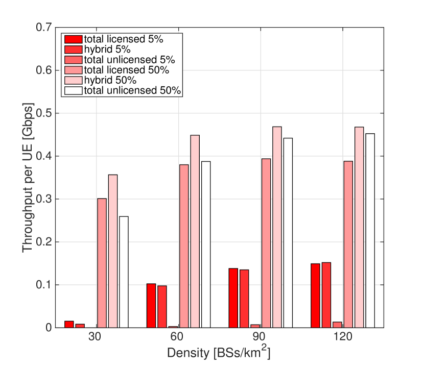
Figure 3: Comparison of the average throughput $\eta$ measured for the hybrid case and the two baselines. Values for the 5-th and 50-th percentiles in case i), where both bands use the same number of antenna elements.

Hybrid access vs. fully unlicensed

On the other hand, we are interested in comparing the performance trends of a hybrid access scheme against that of a fully unlicensed approach. We note that the median user (50%) throughput when adopting a fully unlicensed access strategy increases with the BS density; the gap with respect to the performance obtained through a hybrid scheme reduces until (i) almost overlapping, in Figure 3, and (ii) slightly outperforming it, in Figure 4. However, if we observe the performance trends of the worst-case users (5%), our proposed hybrid access strategy always greatly outperforms the achieved throughput of a fully unlicensed policy.

This preliminary set of results shows that a hybrid allocation procedure can provide a promising tradeoff between fully licensed and fully unlicensed policies. In particular, it can be observed that, for the median user, in most cases (except for low density in case i)) the fully unlicensed policy has better performance than the fully licensed one. The opposite is true for the worst-case users, i.e., the fully unlicensed solution is always much worse that the fully licensed one. On the other hand, our proposed hybrid policy often performs better than both baselines, or it outperforms one and is comparable (or only slightly inferior) to the other, and is therefore able to provide consistently good performance across all users.

V Conclusion

We studied the performance of a hybrid spectrum scheme where exclusive access is used at frequencies in the 20/30 GHz range while spectrum pooling/unlicensed spectrum is used at frequencies around 70 GHz. Our preliminary results show that hybrid spectrum access is a promising approach for mmWave networks and motivate further studies to achieve a more complete understanding of both technical and non technical implications.

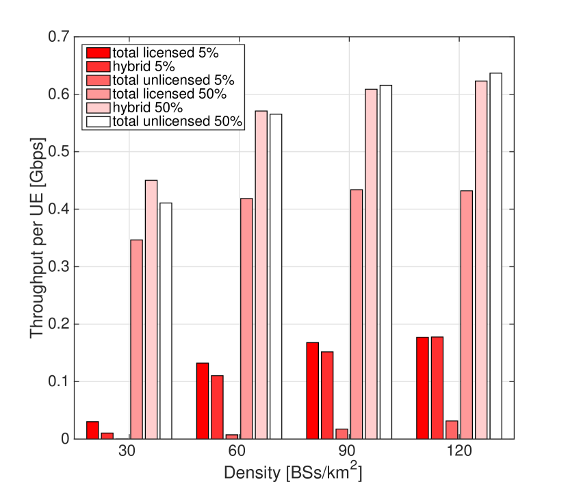
Figure 4: Comparison of the average throughput $\eta$ measured for the hybrid case and the two baselines. Values for the 5-th and 50-th percentiles in case ii), where the carriers use a different number of antenna elements.

References

- [1] METIS, “Deliverable 5.1, intermediate description of spectrum needs and usage principles,” Tech. Rep., 2013.
- [2] F. Boccardi, H. Shokri-Ghadikolaei, G. Fodor, E. Erkip, C. Fischione, M. Kountouris, P. Popovski, and M. Zorzi, “Spectrum Pooling in MmWave Networks: Opportunities, Challenges, and Enablers,” ArXiv e-prints, Mar. 2016. [Online]. Available: https://arxiv.org/abs/1603.01080
- [3] G. Li, T. Irnich, and C. Shi, “Coordination context-based spectrum sharing for 5G millimeter-wave networks,” in IEEE International Conference on Cognitive Radio Oriented Wireless Networks and Communications (CROWNCOM), 2014, pp. 32–38.
- [4] A. K. Gupta, J. G. Andrews, and R. W. H. Jr., “On the Feasibility of Sharing Spectrum Licenses in mmWave Cellular systems,” CoRR, vol. abs/1512.01290, 2015. [Online]. Available: http://arxiv.org/abs/1512.01290
- [5] M. Rebato, M. Mezzavilla, S. Rangan, and M. Zorzi, “Resource Sharing in 5G mmWave Cellular Networks,” in IEEE INFOCOM Millimeter-wave Networking Workshop (mmNet 2016), San Francisco, USA, Apr. 2016.
- [6] M. Akdeniz, Y. Liu, M. Samimi, S. Sun, S. Rangan, T. Rappaport, and E. Erkip, “Millimeter Wave Channel Modeling and Cellular Capacity Evaluation,” IEEE Journal on Selected Areas in Communications, vol. 32, no. 6, pp. 1164–1179, June 2014.
- [7] Y. Azar, G. Wong, K. Wang, R. Mayzus, J. Schulz, H. Zhao, F. Gutierrez, D. Hwang, and T. Rappaport, “28 GHz Propagation Measurements for Outdoor Cellular Communications Using Steerable Beam Antennas in New York City,” in IEEE International Conference on Communications (ICC), June 2013, pp. 5143–5147.
- [8] H. Zhao, R. Mayzus, S. Sun, M. Samimi, J. Schulz, Y. Azar, K. Wang, G. Wong, F. Gutierrez, and T. Rappaport, “28 GHz Millimeter Wave Cellular Communication Measurements for Reflection and Penetration Loss in and Around Buildings in New York City,” in IEEE International Conference on Communications (ICC), June 2013, pp. 5163–5167.
- [9] M. Samimi, K. Wang, Y. Azar, G. Wong, R. Mayzus, H. Zhao, J. Schulz, S. Sun, F. Gutierrez, and T. Rappaport, “28 GHz Angle of Arrival and Angle of Departure Analysis for Outdoor Cellular Communications Using Steerable Beam Antennas in New York City,” in IEEE 77th Vehicular Technology Conference (VTC Spring), June 2013.
- [10] T. S. Rappaport, S. Sun, R. Mayzus, H. Zhao, Y. Azar, K. Wang, G. N. Wong, J. K. Schulz, M. Samimi, and F. Gutierrez, “Millimeter Wave Mobile Communications for 5G Cellular: It Will Work!” IEEE Access, vol. 1, pp. 335–349, 2013.
- [11] M. K. Samimi and T. S. Rappaport, “3-D statistical channel model for millimeter-wave outdoor mobile broadband communications,” in IEEE International Conference on Communications (ICC), June 2015, pp. 2430–2436.