Third-order analysis of pseudopotential lattice Boltzmann model for multiphase flow

Abstract

In this work, a third-order Chapman-Enskog analysis of the multiple-relaxation-time (MRT) pseudopotential lattice Boltzmann (LB) model for multiphase flow is performed for the first time. The leading terms on the interaction force, consisting of an anisotropic and an isotropic term, are successfully identified in the third-order macroscopic equation recovered by the lattice Boltzmann equation (LBE), and then new mathematical insights into the pseudopotential LB model are provided. For the third-order anisotropic term, numerical tests show that it can cause the stationary droplet to become out-of-round, which suggests the isotropic property of the LBE needs to be seriously considered in the pseudopotential LB model. By adopting the classical equilibrium moment or setting the so-called “magic” parameter to $1/12$, the anisotropic term can be eliminated, which is found from the present third-order analysis and also validated numerically. As for the third-order isotropic term, when and only when it is considered, accurate continuum form pressure tensor can be definitely obtained, by which the predicted coexistence densities always agree well with the numerical results. Compared with this continuum form pressure tensor, the classical discrete form pressure tensor is accurate only when the isotropic term is a specific one. At last, in the framework of the present third-order analysis, a consistent scheme for third-order additional term is proposed, which can be used to independently adjust the coexistence densities and surface tension. Numerical tests are subsequently carried out to validate the present scheme.

1 Introduction

Multiphase flows are widely encountered in lots of natural and engineering systems, such as falling raindrop, cloud formation, droplet-based microfluidic, phase-change device, etc. Due to the existence of the deformable phase interface whose position is unknown in advance, numerical simulation of multiphase flow is much more complicated than that of single-phase flow. As a powerful and attractive mesoscopic approach for simulating complex fluid flow problem, the lattice Boltzmann (LB) method has been applied to the simulation of multiphase flow in past years [1, 2, 3, 4]. Generally, the existing LB methods for multiphase flow can be grouped into four major categories: (1) the color-gradient LB method [5, 6, 7, 8], (2) the pseudopotential LB method [9, 10, 11, 12, 13], (3) the free-energy LB method [14, 15, 16, 17], and (4) the kinetic-theory-based LB method [18, 19, 20, 21]. Among these LB methods, the pseudopotential LB method, originally proposed by Shan and Chen [9, 10], is the simplest one in both concept and computation, and thus becomes particularly popular in the LB community for the simulation of multiphase flow.

In the pseudopotential LB model for multiphase flow, an interaction force is introduced to mimic the underlying intermolecular interactions, which are responsible for the formation of multiphase flow. Consequently, phase transition or separation can be automatically achieved, and thus the conventional interface capturing and tracking methods are avoided. Essentially speaking, the interaction force, which is incorporated into the lattice Boltzmann equation (LBE) through a general forcing scheme, can be viewed as a finite-difference gradient operator to recover the non-ideal gas component of the non-monotonic equation of state (EOS) [22] (i.e., $p_{\text{\tiny EOS}}-p^{\text{\tiny ideal}}$, where $p_{\text{\tiny EOS}}$ and $p^{\text{\tiny ideal}}$ denote the non-monotonic EOS and its ideal gas component, respectively). Simultaneously, the interfacial dynamics, such as the non-zero surface tension, are automatically produced by the higher-order terms in the finite-difference gradient operator. Due to such simple and integrated treatments of the interfacial dynamics, some well-known drawbacks exist in the pseudopotential LB model, though its application has been particularly fruitful [23, 24, 25, 26, 27, 28].

One drawback of the pseudopotential LB model is the relatively large spurious current near the curved phase interface, especially at a large density ratio. Shan [22] argued that the spurious current is caused by the insufficient isotropy of the interaction force (as a finite-difference gradient operator), and inferred that the spurious current can be made arbitrarily small by increasing the degree of isotropy of the interaction force, which is realized by counting the interactions beyond nearest-neighbor. Numerical tests show the spurious current is suppressed to some extent by Shan’s method [22, 11], and counting more neighbors will complicate the boundary condition treatment. Sbragaglia et al. [11] investigated the refinement of phase interface and found that the spurious current can be remarkably reduced by widening the phase interface (in lattice units). Afterwards, some more methods were proposed to adjust the interface thickness [29, 30, 31]. Recently, Guo et al. [32] and Xiong and Guo [33] analyzed the force balance condition at the discrete lattice level of LBE, and found that the spurious current is partly caused by the intrinsic force imbalance in the LBE. Besides the above works, some other researches have also been made to shed light on the origin of the spurious current [34] and to provide way to reduce the spurious current [35].

Another two drawbacks of the pseudopotential LB model are the thermodynamic inconsistency (the coexistence densities are inconsistent with the thermodynamic results) and the nonadjustable surface tension (the surface tension cannot be adjusted independently of the coexistence densities). Both of these two drawbacks stem from the simple and integrated treatments of the interfacial dynamics, since the coexistence densities and surface tension are affected, or even determined, by the higher-order terms in the interaction force. In the pseudopotential LB community, it has been widely shown that different forcing schemes for incorporating the interaction force into LBE yield distinctly different coexistence densities (particularly the gas density at a large density ratio) [36, 30, 37, 38]. Li et al. [12] found that the rationale behind this phenomenon is that different forcing schemes produce different additional terms in the recovered macroscopic equation, which have important influences on the interfacial dynamics for multiphase flow, and then they proposed a forcing scheme to alleviate the thermodynamic inconsistency. Following the similar way, some other forcing schemes have been proposed recently [31, 39, 40]. As compared to the thermodynamic inconsistency, the nonadjustable surface tension has not received much attention. In 2007, Sbragaglia et al. [11] first proposed a multirange pseudopotential LB model, where the surface tension can be adjusted independently of the EOS. However, as shown by Huang et al.’s numerical tests [30], the coexistence densities, which are not only determined by the EOS but also affected by the interfacial dynamics, still vary with the adjustment of surface tension. By introducing a source term into LBE to incorporate specific additional term, Li and Luo [41] proposed a nearest-neighbor-based approach to adjust the surface tension independently of the coexistence densities. Similar additional term was also utilized to independently adjust the surface tension in the latter work by Lycett-Brown and Luo [40].

Up to date, the above drawbacks in the pseudopotential LB model have been widely investigated and the corresponding theoretical foundations for the pseudopotential LB model have been further consolidated. However, there still exist some theoretical aspects unclear or inconsistent in the pseudopotential LB model. The isotropic property of the LBE has not been investigated although this aspect of the interaction force has been clearly clarified. Accurate pressure tensor cannot be obtained from the recovered macroscopic equation and the reason is still unclear. Some additional terms, like $\nabla\cdot(h\mathbf{FF})$ ($h$ is a coefficient and $\mathbf{F}$ is the interaction force), should be recovered at the third-order through the Chapman-Enskog analysis, but such terms were inconsistently recovered at the second-order previously. To understand these unclear or inconsistent theoretical aspects, the traditional second-order Chapman-Enskog analysis, which is adopted in nearly all previous works, is insufficient, and higher-order analysis is required. In this work, we target on these theoretical aspects, and perform a third-order Chapman-Enskog analysis of the multiple-relaxation-time (MRT) pseudopotential LB model for multiphase flow. The remainder of the present paper is organized as follows. Section 2 briefly introduces the MRT pseudopotential LB model. Section 3 gives the standard second-order Chapman-Enskog analysis. In Section 4, a third-order Chapman-Enskog analysis of the MRT pseudopotential LB model is performed. In Section 5, the theoretical results of the third-order analysis are discussed detailedly and validated numerically. In Section 6, a consistent scheme for third-order additional term is proposed to independently adjust the coexistence densities and surface tension. At last, a brief conclusion is drawn in Section 7.

2 MRT pseudopotential LB model

Without loss of generality, a two-dimensional nine-velocity (D2Q9) MRT pseudopotential LB model is considered in this work. In the D2Q9 lattice, discrete velocities are given as

$$\mathbf{e}_{i}=\begin{cases}c\big{(}0,\;0\big{)}^{\text{T}},&i=0,\\ c\big{(}\cos[(i-1)\pi/2],\;\sin[(i-1)\pi/2]\big{)}^{\text{T}},&i=1,2,3,4,\\ \sqrt{2}c\big{(}\cos[(2i-1)\pi/4],\;\sin[(2i-1)\pi/4]\big{)}^{\text{T}},&i=5,6,7,8,\\ \end{cases}$$ (1)

where $c=\delta_{x}/\delta_{t}$ is the lattice speed, and $\delta_{x}$ and $\delta_{t}$ are the lattice spacing and time step, respectively. The MRT LBE for the density distribution function $\mathbf{f}(\mathbf{x},t)=\big{[}f_{0}(\mathbf{x},t),\,\cdots,\,f_{8}(\mathbf{x},t)\big{]}^{\text{T}}$ can be decomposed into two sub-steps: the collision step and the streaming step. Generally, the collision step is carried out in the moment space

$$\bar{\mathbf{m}}(\mathbf{x},t)=\mathbf{m}(\mathbf{x},t)-\mathbf{S}\left[\mathbf{m}(\mathbf{x},t)-\mathbf{m}^{\text{eq}}(\mathbf{x},t)\right]+\delta_{t}\left(\mathbf{I}-\dfrac{\mathbf{S}}{2}\right)\mathbf{F}_{m}(\mathbf{x},t),$$ (2)

while the streaming step is carried out in the velocity space

$$f_{i}(\mathbf{x}+\mathbf{e}_{i}\delta_{t},t+\delta_{t})=\bar{f}_{i}(\mathbf{x},t).$$ (3)

Here, $\mathbf{m}(\mathbf{x},t)=\big{[}m_{0}(\mathbf{x},t),\,\cdots,\,m_{8}(\mathbf{x},t)\big{]}^{\text{T}}=\mathbf{M}\mathbf{f}(\mathbf{x},t)$ is the rescaled moment, $\bar{\mathbf{f}}(\mathbf{x},t)=\big{[}\bar{f}_{0}(\mathbf{x},t),\,\cdots,\,\bar{f}_{8}(\mathbf{x},t)\big{]}^{\text{T}}=\mathbf{M}^{-1}\bar{\mathbf{m}}(\mathbf{x},t)$ is post-collision distribution function, $\mathbf{S}=\text{diag}(s_{0},s_{e},s_{\varepsilon},s_{j},s_{q},s_{j},s_{q},s_{p},s_{p})$ is the diagonal relaxation matrix, $\mathbf{I}$ is the unit matrix, $\mathbf{m}^{\text{eq}}(\mathbf{x},t)$ is the equilibrium moment, and $\mathbf{F}_{m}(\mathbf{x},t)$ is the discrete force term. For the D2Q9 lattice, the dimensionless orthogonal transformation matrix $\mathbf{M}$ can be chosen as [42]

$$\mathbf{M}=\left(\begin{array}[]{ccccccccc}1&1&1&1&1&1&1&1&1\\ -4&-1&-1&-1&-1&2&2&2&2\\ 4&-2&-2&-2&-2&1&1&1&1\\ 0&1&0&-1&0&1&-1&-1&1\\ 0&-2&0&2&0&1&-1&-1&1\\ 0&0&1&0&-1&1&1&-1&-1\\ 0&0&-2&0&2&1&1&-1&-1\\ 0&1&-1&1&-1&0&0&0&0\\ 0&0&0&0&0&1&-1&1&-1\end{array}\right).$$ (4)

Different from previous MRT pseudopotential LB models [35, 31, 39], and following the pioneering work by Lallemand and Luo [42], a free parameter $\alpha$ is retained in the equilibrium moment $\mathbf{m}^{\text{eq}}(\mathbf{x},t)$ as follows

$$\mathbf{m}^{\text{eq}}=\left(\rho,\;-2\rho+3\rho\dfrac{|\mathbf{u}|^{2}}{c^{2}},\;\alpha\rho-3\rho\dfrac{|\mathbf{u}|^{2}}{c^{2}},\;\rho\dfrac{u_{x}}{c},\;-\rho\dfrac{u_{x}}{c},\;\rho\dfrac{u_{y}}{c},\;-\rho\dfrac{u_{y}}{c},\;\rho\dfrac{u_{x}^{2}-u_{y}^{2}}{c^{2}},\;\rho\dfrac{u_{x}u_{y}}{c^{2}}\right)^{\text{T}}.$$ (5)

Note that the present equilibrium moment degenerates to the classical one adopted in previous works when $\alpha=1$. The discrete force term in the moment space $\mathbf{F}_{m}(\mathbf{x},t)$ is given as [20, 43]

$$\mathbf{F}_{m}=\left(0,\;6\dfrac{\mathbf{F}\cdot\mathbf{u}}{c^{2}},\;-6\dfrac{\mathbf{F}\cdot\mathbf{u}}{c^{2}},\;\dfrac{F_{x}}{c},\;-\dfrac{F_{x}}{c},\;\dfrac{F_{y}}{c},\;-\dfrac{F_{y}}{c},\;2\dfrac{F_{x}u_{x}-F_{y}u_{y}}{c^{2}},\;\dfrac{F_{x}u_{y}+F_{y}u_{x}}{c^{2}}\right)^{\text{T}}.$$ (6)

The macroscopic variables, density $\rho$ and velocity $\mathbf{u}$, are defined as

$$\rho=\sum\limits_{i=0}^{8}f_{i},\qquad\rho\mathbf{u}=\sum\limits_{i=0}^{8}\mathbf{e}_{i}f_{i}+\dfrac{\delta_{t}}{2}\mathbf{F}.$$ (7)

For the above LB model with a force term, it is well known that no additional term exists in the recovered macroscopic equation at the Navier-Stokes level [44], as will be shown in Section 3.

In the pseudopotential LB model for multiphase flow, the non-monotonic equation of state and the non-zero surface tension are simultaneously produced by the introduction of an interaction force. For the nearest-neighbor interactions on D2Q9 lattice, the interaction force can be expressed as [10, 45]

$$\mathbf{F}(\mathbf{x})=-G\psi(\mathbf{x})\sum\limits_{i=1}^{8}\omega(|\mathbf{e}_{i}\delta_{t}|^{2})\psi(\mathbf{x}+\mathbf{e}_{i}\delta_{t})\mathbf{e}_{i}\delta_{t},$$ (8)

where $\psi(\mathbf{x})$ is the interaction potential (also named as the pseudopotential), $G$ is the interaction strength, and $\omega(|\mathbf{e}_{i}\delta_{t}|^{2})$ are the weights, which are given as $\omega(\delta_{x}^{2})=1/3$ and $\omega(2\delta_{x}^{2})=1/12$ to make $\mathbf{F}(\mathbf{x})$ fourth-order isotropic [45]. Consequently, the following non-monotonic EOS can be obtained [10]

$$p_{\text{\tiny EOS}}=\dfrac{\rho c^{2}}{3}+\dfrac{G\delta_{x}^{2}}{2}\psi^{2},$$ (9)

where $\rho c^{2}/3$ is the ideal gas component ($p^{\text{\tiny ideal}}$) recovered by the LBE. For a prescribed EOS in real application, the interaction potential is inversely calculated by Eq. (9), i.e., $\psi=\sqrt{\raise 1.29167pt\hbox{$2(p_{\text{\tiny EOS}}-\rho c^{2}/3)$}\left/\lower 1.29167pt\hbox{$(G\delta_{x}^{2})$}\right.}$. In this case, $G$ can be chosen arbitrarily as long as the term inside the square root is positive [46]. In the present work, the Carnahan-Starling EOS in thermodynamic theory is taken as an example, which is given as [46, 47]

$$p_{\text{\tiny EOS}}=K\left[\rho RT\dfrac{1+b\rho/4+(b\rho/4)^{2}-(b\rho/4)^{3}}{(1-b\rho/4)^{3}}-a\rho^{2}\right],$$ (10)

where $R$ is the gas constant, $T$ is the temperature, and $a=0.4963R^{2}T_{c}^{2}/p_{c}$ and $b=0.18727RT_{c}/p_{c}$ with $T_{c}$ and $p_{c}$ being the critical temperature and pressure, respectively. Moreover, a scaling factor $K$ is also included in the EOS, which can be used to adjust the interface thickness in the simulation [29, 39].

3 Second-order analysis

To establish a starting point for the third-order Chapman-Enskog analysis, we first perform the standard second-order Chapman-Enskog analysis of the MRT pseudopotential LB model in this section. Through a second-order Taylor series expansion of $f_{i}(\mathbf{x}+\mathbf{e}_{i}\delta_{t},t+\delta_{t})$ centered at $(\mathbf{x},t)$, the streaming step (i.e., Eq. (3)) can be written as

$$f_{i}+\delta_{t}(\partial_{t}+\mathbf{e}_{i}\cdot\nabla)f_{i}+\dfrac{\delta_{t}^{2}}{2}(\partial_{t}+\mathbf{e}_{i}\cdot\nabla)^{2}f_{i}+O(\delta_{t}^{3})=\bar{f}_{i}.$$ (11)

Transforming Eq. (11) into the moment space, and then combining it with the collision step (i.e., Eq. (2)), we obtain

$$(\mathbf{I}\partial_{t}+\mathbf{D})\mathbf{m}+\dfrac{\delta_{t}}{2}(\mathbf{I}\partial_{t}+\mathbf{D})^{2}\mathbf{m}+O(\delta_{t}^{2})=-\dfrac{\mathbf{S}}{\delta_{t}}(\mathbf{m}-\mathbf{m}^{\text{eq}})+\left(\mathbf{I}-\dfrac{\mathbf{S}}{2}\right)\mathbf{F}_{m},$$ (12)

where $\mathbf{D}=\mathbf{M}\big{[}\text{diag}(\mathbf{e}_{0}\cdot\nabla,\,\cdots,\,\mathbf{e}_{8}\cdot\nabla)\big{]}\mathbf{M}^{-1}$. Eq. (12) is called the Taylor series expansion of the MRT LBE in the moment space. Introducing the following Chapman-Enskog expansions [48]

$$\partial_{t}=\sum\limits_{n=1}^{+\infty}\varepsilon^{n}\partial_{tn},\qquad\nabla=\varepsilon\nabla_{1},\qquad f_{i}=\sum\limits_{n=0}^{+\infty}\varepsilon^{n}f_{i}^{(n)},\qquad\mathbf{F}=\varepsilon\mathbf{F}^{(1)},$$ (13)

there have $\mathbf{D}=\varepsilon\mathbf{D}_{1}$, $\mathbf{m}=\sum\nolimits_{n=0}^{+\infty}\varepsilon^{n}\mathbf{m}^{(n)}$, and $\mathbf{F}_{m}=\varepsilon\mathbf{F}_{m}^{(1)}$, where $\varepsilon$ is the small expansion parameter. Substituting these Chapman-Enskog expansions into Eq. (12), we can rewrite Eq. (12) in the consecutive orders of $\varepsilon$ as

$$\varepsilon^{0}:\;\mathbf{m}^{(0)}=\mathbf{m}^{\text{eq}},$$ (14a)

$$\varepsilon^{1}:\;(\mathbf{I}\partial_{t1}+\mathbf{D}_{1})\mathbf{m}^{(0)}-\mathbf{F}_{m}^{(1)}=-\dfrac{\mathbf{S}}{\delta_{t}}\left(\mathbf{m}^{(1)}+\dfrac{\delta_{t}}{2}\mathbf{F}_{m}^{(1)}\right),$$ (14b)

$$\varepsilon^{2}:\;\partial_{t2}\mathbf{m}^{(0)}+(\mathbf{I}\partial_{t1}+\mathbf{D}_{1})\left(\mathbf{I}-\dfrac{\mathbf{S}}{2}\right)\left(\mathbf{m}^{(1)}+\dfrac{\delta_{t}}{2}\mathbf{F}_{m}^{(1)}\right)=-\dfrac{\mathbf{S}}{\delta_{t}}\mathbf{m}^{(2)},$$ (14c)

where the first-order ($\varepsilon^{1}$) equation has been used to simplify the second-order ($\varepsilon^{2}$) equation.

To deduce the macroscopic equation, we extract the equations for the conserved moments ($m_{0}$, $m_{3}$, and $m_{5}$) from Eq. (14) as

$$\varepsilon^{0}:\;\begin{cases}m_{0}^{(0)}=m_{0}^{\text{eq}},\\ m_{3}^{(0)}=m_{3}^{\text{eq}},\\ m_{5}^{(0)}=m_{5}^{\text{eq}},\end{cases}$$ (15a)

$$\varepsilon^{1}:\;\begin{cases}\partial_{t1}m_{0}^{(0)}+c\partial_{x1}m_{3}^{(0)}+c\partial_{y1}m_{5}^{(0)}-F_{m0}^{(1)}=-\tfrac{s_{0}}{\delta_{t}}\left(m_{0}^{(1)}+\tfrac{\delta_{t}}{2}F_{m0}^{(1)}\right),\\ \partial_{t1}m_{3}^{(0)}+c\partial_{x1}\left(\tfrac{2}{3}m_{0}^{(0)}+\tfrac{1}{6}m_{1}^{(0)}+\tfrac{1}{2}m_{7}^{(0)}\right)+c\partial_{y1}m_{8}^{(0)}-F_{m3}^{(1)}=-\tfrac{s_{j}}{\delta_{t}}\left(m_{3}^{(1)}+\tfrac{\delta_{t}}{2}F_{m3}^{(1)}\right),\\ \partial_{t1}m_{5}^{(0)}+c\partial_{x1}m_{8}^{(0)}+c\partial_{y1}\left(\tfrac{2}{3}m_{0}^{(0)}+\tfrac{1}{6}m_{1}^{(0)}-\tfrac{1}{2}m_{7}^{(0)}\right)-F_{m5}^{(1)}=-\tfrac{s_{j}}{\delta_{t}}\left(m_{5}^{(1)}+\tfrac{\delta_{t}}{2}F_{m5}^{(1)}\right),\end{cases}$$ (15b)

$$\varepsilon^{2}:\;\begin{cases}\left(\begin{aligned} &\partial_{t2}m_{0}^{(0)}+\partial_{t1}\left(1-\tfrac{s_{0}}{2}\right)\left(m_{0}^{(1)}+\tfrac{\delta_{t}}{2}F_{m0}^{(1)}\right)+\\ &c\partial_{x1}\left(1-\tfrac{s_{j}}{2}\right)\left(m_{3}^{(1)}+\tfrac{\delta_{t}}{2}F_{m3}^{(1)}\right)+c\partial_{y1}\left(1-\tfrac{s_{j}}{2}\right)\left(m_{5}^{(1)}+\tfrac{\delta_{t}}{2}F_{m5}^{(1)}\right)\end{aligned}\right)=-\tfrac{s_{0}}{\delta_{t}}m_{0}^{(2)},\\ \left(\begin{aligned} &\partial_{t2}m_{3}^{(0)}+\partial_{t1}\left(1-\tfrac{s_{j}}{2}\right)\left(m_{3}^{(1)}+\tfrac{\delta_{t}}{2}F_{m3}^{(1)}\right)+c\partial_{y1}\left(1-\tfrac{s_{p}}{2}\right)\left(m_{8}^{(1)}+\tfrac{\delta_{t}}{2}F_{m8}^{(1)}\right)+\\ &c\partial_{x1}\left[\tfrac{2}{3}\left(1-\tfrac{s_{0}}{2}\right)\left(m_{0}^{(1)}+\tfrac{\delta_{t}}{2}F_{m0}^{(1)}\right)+\tfrac{1}{6}\left(1-\tfrac{s_{e}}{2}\right)\left(m_{1}^{(1)}+\tfrac{\delta_{t}}{2}F_{m1}^{(1)}\right)+\tfrac{1}{2}\left(1-\tfrac{s_{p}}{2}\right)\left(m_{7}^{(1)}+\tfrac{\delta_{t}}{2}F_{m7}^{(1)}\right)\right]\end{aligned}\right)=-\tfrac{s_{j}}{\delta_{t}}m_{3}^{(2)},\\ \left(\begin{aligned} &\partial_{t2}m_{5}^{(0)}+\partial_{t1}\left(1-\tfrac{s_{j}}{2}\right)\left(m_{5}^{(1)}+\tfrac{\delta_{t}}{2}F_{m5}^{(1)}\right)+c\partial_{x1}\left(1-\tfrac{s_{p}}{2}\right)\left(m_{8}^{(1)}+\tfrac{\delta_{t}}{2}F_{m8}^{(1)}\right)+\\ &c\partial_{y1}\left[\tfrac{2}{3}\left(1-\tfrac{s_{0}}{2}\right)\left(m_{0}^{(1)}+\tfrac{\delta_{t}}{2}F_{m0}^{(1)}\right)+\tfrac{1}{6}\left(1-\tfrac{s_{e}}{2}\right)\left(m_{1}^{(1)}+\tfrac{\delta_{t}}{2}F_{m1}^{(1)}\right)-\tfrac{1}{2}\left(1-\tfrac{s_{p}}{2}\right)\left(m_{7}^{(1)}+\tfrac{\delta_{t}}{2}F_{m7}^{(1)}\right)\right]\end{aligned}\right)=-\tfrac{s_{j}}{\delta_{t}}m_{5}^{(2)}.\end{cases}$$ (15c)

Considering $m_{0}=\rho$, $m_{3}=\rho u_{x}/c-\tfrac{\delta_{t}}{2}F_{x}/c$, and $m_{5}=\rho u_{y}/c-\tfrac{\delta_{t}}{2}F_{y}/c$ (see Eq. (7)), Eq. (15a) indicates that

$$\begin{cases}m_{0}^{(1)}+\tfrac{\delta_{t}}{2}F_{m0}^{(1)}=0,\qquad m_{0}^{(n)}=0\;(\forall n\geq 2),\\ m_{3}^{(1)}+\tfrac{\delta_{t}}{2}F_{m3}^{(1)}=0,\qquad m_{3}^{(n)}=0\;(\forall n\geq 2),\\ m_{5}^{(1)}+\tfrac{\delta_{t}}{2}F_{m5}^{(1)}=0,\qquad m_{5}^{(n)}=0\;(\forall n\geq 2).\end{cases}$$ (16)

Therefore, the first-order equation (i.e., Eq. (15b)) can be simplified as

$$\varepsilon^{1}:\;\begin{cases}\partial_{t1}\rho+\partial_{x1}(\rho u_{x})+\partial_{y1}(\rho u_{y})=0,\\ \partial_{t1}(\rho u_{x})+\partial_{x1}(\rho u_{x}^{2})+\partial_{y1}(\rho u_{x}u_{y})=-\partial_{x1}(\tfrac{1}{3}\rho c^{2})+F_{x}^{(1)},\\ \partial_{t1}(\rho u_{y})+\partial_{x1}(\rho u_{x}u_{y})+\partial_{y1}(\rho u_{y}^{2})=-\partial_{y1}(\tfrac{1}{3}\rho c^{2})+F_{y}^{(1)}.\end{cases}$$ (17)

Based on Eq. (17), the following relation can be obtained

$$\begin{split}\partial_{t1}(\rho\mathbf{uu})&=[\partial_{t1}(\rho\mathbf{u})]\mathbf{u}+\mathbf{u}[\partial_{t1}(\rho\mathbf{u})]-\mathbf{uu}(\partial_{t1}\rho)\\ &=-\tfrac{1}{3}c^{2}[(\nabla_{1}\rho)\mathbf{u}+\mathbf{u}(\nabla_{1}\rho)]+\mathbf{F}^{(1)}\mathbf{u}+\mathbf{u}\mathbf{F}^{(1)}+O(|\mathbf{u}|^{3}),\end{split}$$ (18)

where the cubic term of velocity will be neglected with the low Mach number condition. In order to simplify the second-order equation (i.e., Eq. (15c)), the involved first-order terms on the non-conserved moments, i.e., $m_{1}^{(1)}+\tfrac{\delta_{t}}{2}F_{m1}^{(1)}$, $m_{7}^{(1)}+\tfrac{\delta_{t}}{2}F_{m7}^{(1)}$, and $m_{8}^{(1)}+\tfrac{\delta_{t}}{2}F_{m8}^{(1)}$, should be calculated firstly. These first-order terms are obtained from Eq. (14b) and then simplified with the aid of Eqs. (14a) and (18) as:

$$\begin{split}-\tfrac{s_{e}}{\delta_{t}}\left(m_{1}^{(1)}+\tfrac{\delta_{t}}{2}F_{m1}^{(1)}\right)&=\partial_{t1}m_{1}^{(0)}+c\partial_{x1}\left(m_{3}^{(0)}+m_{4}^{(0)}\right)+c\partial_{y1}\left(m_{5}^{(0)}+m_{6}^{(0)}\right)-F_{m1}^{(1)}\\ &\approx 2\rho(\partial_{x1}u_{x}+\partial_{y1}u_{y}),\end{split}$$ (19a)

$$\begin{split}-\tfrac{s_{p}}{\delta_{t}}\left(m_{7}^{(1)}+\tfrac{\delta_{t}}{2}F_{m7}^{(1)}\right)&=\partial_{t1}m_{7}^{(0)}+c\partial_{x1}\left(\tfrac{1}{3}m_{3}^{(0)}-\tfrac{1}{3}m_{4}^{(0)}\right)-c\partial_{y1}\left(\tfrac{1}{3}m_{5}^{(0)}-\tfrac{1}{3}m_{6}^{(0)}\right)-F_{m7}^{(1)}\\ &\approx\tfrac{2}{3}\rho(\partial_{x1}u_{x}-\partial_{y1}u_{y}),\end{split}$$ (19b)

$$\begin{split}-\tfrac{s_{p}}{\delta_{t}}\left(m_{8}^{(1)}+\tfrac{\delta_{t}}{2}F_{m8}^{(1)}\right)&=\partial_{t1}m_{8}^{(0)}+c\partial_{x1}\left(\tfrac{2}{3}m_{5}^{(0)}+\tfrac{1}{3}m_{6}^{(0)}\right)+c\partial_{y1}\left(\tfrac{2}{3}m_{3}^{(0)}+\tfrac{1}{3}m_{4}^{(0)}\right)-F_{m8}^{(1)}\\ &\approx\tfrac{1}{3}\rho(\partial_{x1}u_{y}+\partial_{y1}u_{x}),\end{split}$$ (19c)

where the sign “ $\approx$ ” means the cubic term of velocity is neglected. With the aid of Eqs. (14a), (16), and (19), the second-order equation (i.e., Eq. (15c)) can be finally simplified as

$$\varepsilon^{2}:\;\begin{cases}\partial_{t2}\rho=0,\\ \partial_{t2}(\rho u_{x})=\partial_{x1}[\rho\nu(\partial_{x1}u_{x}-\partial_{y1}u_{y})]+\partial_{y1}[\rho\nu(\partial_{y1}u_{x}+\partial_{x1}u_{y})]+\partial_{x1}[\rho\varsigma(\partial_{x1}u_{x}+\partial_{y1}u_{y})],\\ \partial_{t2}(\rho u_{y})=\partial_{x1}[\rho\nu(\partial_{x1}u_{y}+\partial_{y1}u_{x})]+\partial_{y1}[\rho\nu(\partial_{y1}u_{y}-\partial_{x1}u_{x})]+\partial_{y1}[\rho\varsigma(\partial_{x1}u_{x}+\partial_{y1}u_{y})],\end{cases}$$ (20)

where $\nu=c^{2}\delta_{t}(s_{p}^{-1}-0.5)/3$ is the kinetic viscosity, $\varsigma=c^{2}\delta_{t}(s_{e}^{-1}-0.5)/3$ is the bulk viscosity. Combining the first- and second-order equations (i.e., Eqs. (17) and (20)), the following macroscopic equation at the Navier-Stokes level (second-order) can be recovered

$$\begin{cases}\partial_{t}\rho+\nabla\cdot(\rho\mathbf{u})=0,\\ \partial_{t}(\rho\mathbf{u})+\nabla\cdot(\rho\mathbf{uu})=-\nabla(\tfrac{1}{3}\rho c^{2})+\mathbf{F}+\nabla\cdot\big{\{}\rho\nu[\nabla\mathbf{u}+\mathbf{u}\nabla-(\nabla\cdot\mathbf{u})\mathbf{I}]\big{\}}+\nabla(\rho\varsigma\nabla\cdot\mathbf{u}).\end{cases}$$ (21)

From the above second-order Chapman-Enskog analysis, we can see that the free parameter $\alpha$ makes no difference to the recovered macroscopic equation at the Navier-Stokes level. Moreover, the force term is correctly recovered, i.e., no discrete lattice effect exists.

4 Third-order analysis

To identify the higher-order terms in the recovered macroscopic equation, a third-order Chapman-Enskog analysis of the MRT pseudopotential LB model is carried out in this section. Performing the Taylor series expansion of the streaming step (i.e., Eq. (3)) to third-order, and then transforming the result into the moment space and combining it with the collision step (i.e., Eq. (2)), the following Taylor series expansion of the MRT LBE in the moment space can be obtained

$$(\mathbf{I}\partial_{t}+\mathbf{D})\mathbf{m}+\dfrac{\delta_{t}}{2}(\mathbf{I}\partial_{t}+\mathbf{D})^{2}\mathbf{m}+\dfrac{\delta_{t}^{2}}{6}(\mathbf{I}\partial_{t}+\mathbf{D})^{3}\mathbf{m}+O(\delta_{t}^{3})=-\dfrac{\mathbf{S}}{\delta_{t}}(\mathbf{m}-\mathbf{m}^{\text{eq}})+\left(\mathbf{I}-\dfrac{\mathbf{S}}{2}\right)\mathbf{F}_{m}.$$ (22)

With the Chapman-Enskog expansions given by Eq. (13), Eq. (22) can be rewritten in the consecutive orders of $\varepsilon$ as

$$\varepsilon^{0}:\;\mathbf{m}^{(0)}=\mathbf{m}^{\text{eq}},$$ (23a)

$$\varepsilon^{1}:\;(\mathbf{I}\partial_{t1}+\mathbf{D}_{1})\mathbf{m}^{(0)}-\mathbf{F}_{m}^{(1)}=-\dfrac{\mathbf{S}}{\delta_{t}}\left(\mathbf{m}^{(1)}+\dfrac{\delta_{t}}{2}\mathbf{F}_{m}^{(1)}\right),$$ (23b)

$$\varepsilon^{2}:\;\partial_{t2}\mathbf{m}^{(0)}+(\mathbf{I}\partial_{t1}+\mathbf{D}_{1})\mathbf{m}^{(1)}+\dfrac{\delta_{t}}{2}(\mathbf{I}\partial_{t1}+\mathbf{D}_{1})^{2}\mathbf{m}^{(0)}=-\dfrac{\mathbf{S}}{\delta_{t}}\mathbf{m}^{(2)},$$ (23c)

$$\varepsilon^{3}:\;\left(\begin{aligned} &\partial_{t3}\mathbf{m}^{(0)}+\partial_{t2}\mathbf{m}^{(1)}+(\mathbf{I}\partial_{t1}+\mathbf{D}_{1})\mathbf{m}^{(2)}+\delta_{t}(\mathbf{I}\partial_{t1}+\mathbf{D}_{1})\partial_{t2}\mathbf{m}^{(0)}+\\ &\dfrac{\delta_{t}}{2}(\mathbf{I}\partial_{t1}+\mathbf{D}_{1})^{2}\mathbf{m}^{(1)}+\dfrac{\delta_{t}^{2}}{6}(\mathbf{I}\partial_{t1}+\mathbf{D}_{1})^{3}\mathbf{m}^{(0)}\end{aligned}\right)=-\dfrac{\mathbf{S}}{\delta_{t}}\mathbf{m}^{(3)}.$$ (23d)

Here, the equations at the orders of $\varepsilon^{0}$, $\varepsilon^{1}$, and $\varepsilon^{2}$ (i.e., Eqs. (23a), (23b), and (23c)) are identical to those in the second-order analysis (i.e., Eqs. (14a), (14b), and (14c)). Therefore, at the Navier-Stokes level, Eq. (21) can also be recovered from Eq. (23). From Eq. (23), we can see that the equation at the order of $\varepsilon^{3}$ (i.e., Eq. (23d)) is much more complicated than the equations at the lower-order. Proceeding along the general way, deducing the corresponding macroscopic equation from Eq. (23d) is difficult and rather cumbersome, and will lead to the Burnett level equation. This is clearly unnecessary and not the desired result in this work.

As it is well known, the second-order Chapman-Enskog analysis is sufficient for single-phase flow, and the main difference between the single-phase and multiphase flows is the large density gradient near the phase interface. In the pseudopotential LB model for multiphase flow, such density gradient is directly caused by the interaction force and is irrelevant to time and velocity. Therefore, the goal of the present third-order analysis is to identify the time- and velocity-independent leading terms on the interaction force at the third-order. Keeping this goal in mind, we can consider a steady and stationary situation for the sake of simplicity. For the steady situation, all the time derivative terms are zero, and then Eq. (23) can be simplified as

$$\varepsilon^{0}:\;\mathbf{m}^{(0)}=\mathbf{m}^{\text{eq}},$$ (24a)

$$\varepsilon^{1}:\;\partial_{t1}\mathbf{m}^{(0)}+\mathbf{D}_{1}\mathbf{m}^{(0)}-\mathbf{F}_{m}^{(1)}=-\dfrac{\mathbf{S}}{\delta_{t}}\left(\mathbf{m}^{(1)}+\dfrac{\delta_{t}}{2}\mathbf{F}_{m}^{(1)}\right),$$ (24b)

$$\varepsilon^{2}:\;\partial_{t2}\mathbf{m}^{(0)}-\delta_{t}\mathbf{D}_{1}\left(\mathbf{S}^{-1}-\dfrac{\mathbf{I}}{2}\right)\left(\mathbf{D}_{1}\mathbf{m}^{(0)}-\mathbf{F}_{m}^{(1)}\right)=-\dfrac{\mathbf{S}}{\delta_{t}}\mathbf{m}^{(2)},$$ (24c)

$$\varepsilon^{3}:\;\partial_{t3}\mathbf{m}^{(0)}+\delta_{t}^{2}\left[\mathbf{D}_{1}\left(\mathbf{S}^{-1}-\dfrac{\mathbf{I}}{2}\right)\mathbf{D}_{1}\left(\mathbf{S}^{-1}-\dfrac{\mathbf{I}}{2}\right)\left(\mathbf{D}_{1}\mathbf{m}^{(0)}-\mathbf{F}_{m}^{(1)}\right)-\dfrac{1}{12}\mathbf{D}_{1}^{3}\mathbf{m}^{(0)}\right]=-\dfrac{\mathbf{S}}{\delta_{t}}\mathbf{m}^{(3)},$$ (24d)

where the lower-order equations have been used to simplify the higher-order equations. Note that the terms $\partial_{t1}\mathbf{m}^{(0)}$, $\partial_{t2}\mathbf{m}^{(0)}$, and $\partial_{t3}\mathbf{m}^{(0)}$ are reserved in Eq. (24) though they are equal to zero. These time derivative terms act as a gauge to avoid the wrong scaling among the equations at different orders. As for the stationary situation, the velocity is zero, i.e., $\mathbf{u}=\mathbf{0}$.

Similar to the second-order analysis, the equations for the conserved moments ($m_{0}$, $m_{3}$, and $m_{5}$) are extracted from Eq. (24) to deduce the macroscopic equation. The zeroth-order ($\varepsilon^{0}$) equations for the conserved moments in Eq. (24a) are

$$\varepsilon^{0}:\;\begin{cases}m_{0}^{(0)}=m_{0}^{\text{eq}},\\ m_{3}^{(0)}=m_{3}^{\text{eq}},\\ m_{5}^{(0)}=m_{5}^{\text{eq}},\end{cases}$$ (25)

which indicates that

$$\begin{cases}m_{0}^{(1)}+\tfrac{\delta_{t}}{2}F_{m0}^{(1)}=0,\qquad m_{0}^{(n)}=0\;(\forall n\geq 2),\\ m_{3}^{(1)}+\tfrac{\delta_{t}}{2}F_{m3}^{(1)}=0,\qquad m_{3}^{(n)}=0\;(\forall n\geq 2),\\ m_{5}^{(1)}+\tfrac{\delta_{t}}{2}F_{m5}^{(1)}=0,\qquad m_{5}^{(n)}=0\;(\forall n\geq 2).\end{cases}$$ (26)

With the aid of Eqs. (24a) and (26), the first-order ($\varepsilon^{1}$) equations for the conserved moments in Eq. (24b) are

$$\varepsilon^{1}:\;\begin{cases}\partial_{t1}\rho=0,\\ \partial_{t1}(\rho u_{x})=-\partial_{x1}(\tfrac{1}{3}\rho c^{2})+F_{x}^{(1)},\\ \partial_{t1}(\rho u_{y})=-\partial_{y1}(\tfrac{1}{3}\rho c^{2})+F_{y}^{(1)}.\end{cases}$$ (27)

Similarly, the second-order ($\varepsilon^{2}$) equations for the conserved moments in Eq. (24c) are

$$\varepsilon^{2}:\;\begin{cases}\partial_{t2}\rho=0,\\ \partial_{t2}(\rho u_{x})=0,\\ \partial_{t2}(\rho u_{y})=0.\end{cases}$$ (28)

To simplify the descriptions in the following, we introduce $\text{diag}(\sigma_{0},\sigma_{e},\sigma_{\varepsilon},\sigma_{j},\sigma_{q},\sigma_{j},\sigma_{q},\sigma_{p},\sigma_{p})=\mathbf{S}^{-1}-\mathbf{I}/2$. After some lengthy algebra, the third-order ($\varepsilon^{3}$) equations for the conserved moments in Eq. (24d) are

$$\varepsilon^{3}:\;\begin{cases}\partial_{t3}\rho=0,\\ \partial_{t3}(\rho u_{x})=-\delta_{t}^{2}c^{2}\left[\dfrac{2(\alpha-1)(\sigma_{e}\sigma_{q}-\sigma_{p}\sigma_{q})-1}{12}\left(\partial_{x1}^{2}F_{x}^{(1)}+\partial_{y1}^{2}F_{x}^{(1)}\right)+\dfrac{(\alpha-1)(12\sigma_{p}\sigma_{q}-1)}{12}\partial_{y1}^{2}F_{x}^{(1)}\right],\\ \partial_{t3}(\rho u_{y})=-\delta_{t}^{2}c^{2}\left[\dfrac{2(\alpha-1)(\sigma_{e}\sigma_{q}-\sigma_{p}\sigma_{q})-1}{12}\left(\partial_{x1}^{2}F_{y}^{(1)}+\partial_{y1}^{2}F_{y}^{(1)}\right)+\dfrac{(\alpha-1)(12\sigma_{p}\sigma_{q}-1)}{12}\partial_{x1}^{2}F_{y}^{(1)}\right].\end{cases}$$ (29)

Combining the first-, second-, and third-order equations (i.e., Eqs. (27), (28), and (29)) together, we finally obtain the following third-order macroscopic equation

$$\begin{cases}\partial_{t}\rho=0,\\ \partial_{t}(\rho\mathbf{u})=-\nabla(\tfrac{1}{3}\rho c^{2})+\mathbf{F}+\mathbf{R}_{\text{iso}}+\mathbf{R}_{\text{aniso}},\end{cases}$$ (30)

where $\mathbf{R}_{\text{iso}}$ and $\mathbf{R}_{\text{aniso}}$ are the third-order isotropic and anisotropic terms that are expressed as

$$\mathbf{R}_{\text{iso}}=-\delta_{t}^{2}c^{2}\dfrac{2(\alpha-1)(\sigma_{e}\sigma_{q}-\sigma_{p}\sigma_{q})-1}{12}\nabla\cdot\nabla\mathbf{F},$$ (31a)

$$\mathbf{R}_{\text{aniso}}=-\delta_{t}^{2}c^{2}\dfrac{(\alpha-1)(12\sigma_{p}\sigma_{q}-1)}{12}\left(\partial_{y}^{2}F_{x},\;\partial_{x}^{2}F_{y}\right)^{\text{T}}.$$ (31b)

From the above third-order Chapman-Enskog analysis, we can see that the time- and velocity-independent leading terms on the interaction force definitely exist in the recovered macroscopic equation at the third-order, and the free parameter $\alpha$ has crucial influence on these third-order terms. Note that the above third-order terms still exist for the general situation, even though they are identified under a specific condition.

5 Discussions and validations

In this section, the theoretical results of the present third-order Chapman-Enskog analysis will be discussed detailedly and validated numerically. Firstly, the isotropic property of the LBE is investigated, with a focus on the third-order anisotropic term. Then, the determination of the pressure tensor, which is of crucial importance for multiphase flow, is analyzed, with a focus on the third-order isotropic term. For the numerical validations, the basic simulation parameters are set as $\delta_{x}=1$, $\delta_{t}=1$, $G=-1$, $a=1$, $b=4$, $R=1$, and $K=1$, while the rest simulation parameters will be given individually for different cases.

5.1 Isotropic property of the LBE

At the second-order (Navier-Stokes level), the recovered macroscopic equation is always isotropic (see Eq. (21)). However, at the third-order, anisotropic term $\mathbf{R}_{\text{aniso}}$ is recovered by the LBE in the macroscopic momentum equation (see Eq. (30)). To show the effect of such anisotropic term on multiphase flow, numerical simulations of stationary droplet are carried out on a $N_{x}\times N_{y}=128\times 128$ lattice with periodic boundary conditions in both $x$ and $y$ directions. The relaxation parameters are set as $s_{0}=s_{j}=s_{p}=s_{q}=s_{e}=s_{\varepsilon}=1/\tau$. Here, $\tau$ is the dimensionless relaxation time. The temperature is chosen as $T=0.9T_{c}$, which indicates that the thermodynamic gas and liquid densities given by the Maxwell construction are $\rho_{g}^{\text{thermo}}=4.5435\times 10^{-2}$ and $\rho_{l}^{\text{thermo}}=2.4806\times 10^{-1}$, respectively. In the simulation, the density and velocity fields are initialized as

$$\rho(\mathbf{x})=\dfrac{\rho_{g}^{\text{thermo}}+\rho_{l}^{\text{thermo}}}{2}+\dfrac{\rho_{g}^{\text{thermo}}-\rho_{l}^{\text{thermo}}}{2}\tanh\dfrac{2(|\mathbf{x}-\mathbf{x}_{c}|-r_{0})}{W},$$ (32a)

$$\mathbf{u}(\mathbf{x})=\mathbf{0},$$ (32b)

where $\mathbf{x}_{c}=\tfrac{\delta_{x}}{2}(N_{x},\,N_{y})^{\text{T}}$ is the central position of the computational domain, $W=5\delta_{x}$ is the initial interface width, and $r_{0}=\tfrac{\delta_{x}}{4}N_{x}$ is the initial droplet radius. Fig. 1 shows the steady-state density contours of the droplet for varied $\alpha$ and different $\tau$. It can be clearly seen that when $\alpha\neq 1$ (i.e., $\mathbf{R}_{\text{aniso}}\neq\mathbf{0}$, see Eq. (31b)), the droplet becomes out-of-round and its shape is $\tau\text{-dependent}$; when $\alpha=1$ (i.e., $\mathbf{R}_{\text{aniso}}=\mathbf{0}$, see Eq. (31b)), the shape of droplet is independent of $\tau$ and keeps circular consistently. These results suggest that the third-order anisotropic term recovered by the LBE has important influence on multiphase flow and must be eliminated in real application, which also indicate that the isotropy of the LBE should be third-order at least in the pseudopotential LB model for multiphase flow.

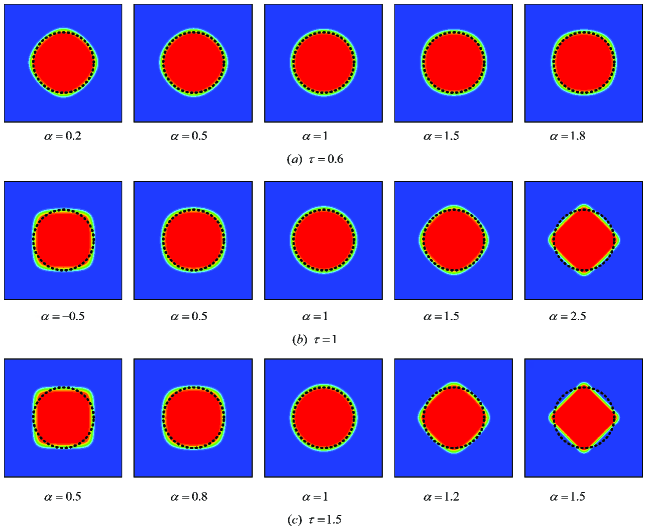
Figure 1: Steady-state density contours of the stationary droplet for varied $\alpha$ and different $\tau$. The inserted dashed circle is the initial shape of the stationary droplet.

The present third-order analysis shows that the third-order anisotropic term $\mathbf{R}_{\text{aniso}}$ is eliminated when $\alpha=1$ (see Eq. (31b)), which means that the general equilibrium moment given by Eq. (5) degenerates to the classical one adopted in previous works. At the same time, it is interesting to find from Eq. (31b) that by setting a “magic” parameter to $1/12$ as follows

$${\it\Lambda}=\sigma_{p}\sigma_{q}=\left(\dfrac{1}{s_{p}}-\dfrac{1}{2}\right)\left(\dfrac{1}{s_{q}}-\dfrac{1}{2}\right)\equiv\dfrac{1}{12},$$ (33)

the anisotropic term $\mathbf{R}_{\text{aniso}}$ can also be eliminated. To validate this point, the same numerical simulations of stationary droplet are carried out except that the relaxation parameters are set as: $s_{0}=s_{j}=s_{p}=s_{e}=s_{\varepsilon}=1/\tau$ and $s_{q}=1/[0.5+{\it\Lambda}/(s_{p}^{-1}-0.5)]$ with ${\it\Lambda}\equiv 1/12$. The steady-state density contours of the droplet are shown in Fig. 2. As expected, the final shape of droplet is circular perfectly for all involved $\alpha$ (including $\alpha\neq 1$) and different $\tau$, which validates the successful elimination of $\mathbf{R}_{\text{aniso}}$ by setting ${\it\Lambda}\equiv 1/12$ and also demonstrates the effectiveness of the present third-order analysis. The above numerical simulations clearly show the necessity of eliminating the third-order anisotropic term $\mathbf{R}_{\text{aniso}}$. Similarly, the third-order isotropic term $\mathbf{R}_{\text{iso}}$ needs to be considered as well, which will be discussed in the next section.

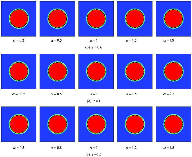
Figure 2: Steady-state density contours of the stationary droplet for varied $\alpha$ and different $\tau$ when the “magic” parameter ${\it\Lambda}\equiv 1/12$. The inserted dashed circle is the initial shape of the stationary droplet.

At the end of this section, a further discussion on the isotropic property of the pseudopotential LB model is deserved. It is well known that the interaction force given by Eq. (8) is fourth-order isotropic, and increasing the degree of isotropy of the interaction force can help to reduce the spurious current [22]. According to the discussion on the third-order anisotropic term recovered by the LBE in this section, the isotropic property of the LBE also has significant influence on multiphase flow in the pseudopotential LB model. Considering the LBE on D2Q9 lattice can achieve fourth-order isotropy at most, some anisotropic terms will emerge in the recovered macroscopic equation at the fifth-order, even though the interaction force is infinite-order isotropic. These higher-order anisotropic terms intrinsically recovered by the LBE will produce some spurious current inevitably. Therefore, the spurious current is partly caused by the finite-order isotropy of the LBE on a discrete lattice, which was not realized previously, and it cannot be made arbitrarily small just by increasing the degree of isotropy of the interaction force.

5.2 Determination of the pressure tensor

In the pseudopotential LB model for multiphase flow, determination of the pressure tensor is of crucial importance. Many macroscopic properties, such as the coexistence densities, can be predicted analytically by the pressure tensor. Generally, the pressure tensor can be determined in two forms: the continuum form pressure tensor and the discrete form pressure tensor. In the pseudopotential LB community, it is well known that the continuum form pressure tensor, which is obtained from the macroscopic equation recovered through the Chapman-Enskog analysis, is inaccurate in predicting the macroscopic properties, and the discrete form pressure tensor, which is exactly constructed on the discrete lattice, should be used for the predictions. For the nearest-neighbor interactions given by Eq. (8), the discrete form pressure tensor is given as [45, 49]

$$\mathbf{P}^{\text{discrete}}(\mathbf{x})=\dfrac{\rho(\mathbf{x})c^{2}}{3}\mathbf{I}+\dfrac{G}{2}\psi(\mathbf{x})\sum\limits_{i=1}^{8}\omega(|\mathbf{e}_{i}\delta_{t}|^{2})\psi(\mathbf{x}+\mathbf{e}_{i}\delta_{t})\mathbf{e}_{i}\delta_{t}\mathbf{e}_{i}\delta_{t}.$$ (34)

Performing the Taylor series expansion of $\psi(\mathbf{x}+\mathbf{e}_{i}\delta_{t})$ centered at $\mathbf{x}$, Eq. (34) can be further expressed as

$$\mathbf{P}^{\text{discrete}}=\left(\dfrac{\rho c^{2}}{3}+\dfrac{G\delta_{x}^{2}}{2}\psi^{2}+\dfrac{G\delta_{x}^{4}}{12}\psi\nabla\cdot\nabla\psi\right)\mathbf{I}+\dfrac{G\delta_{x}^{4}}{6}\psi\nabla\nabla\psi+O(\nabla^{4}),$$ (35)

where the higher-order terms are anisotropic and will be neglected. To determine the coexistence densities, a steady-state one-dimensional flat interface along $y$ direction can be considered. Then, the normal pressure $P_{n}^{\text{discrete}}$ given by Eq. (35) is

$$P_{n}^{\text{discrete}}=P_{xx}=\dfrac{\rho c^{2}}{3}+\dfrac{G\delta_{x}^{2}}{2}\psi^{2}+\dfrac{G\delta_{x}^{4}}{4}\psi\dfrac{d^{2}\psi}{dx^{2}}.$$ (36)

According to Eq. (36) and after some algebra, the following integral equation, which is called the mechanical stability condition, can be obtained [10, 45]

$$\int_{\rho_{g}}^{\rho_{l}}\left(p_{0}-\dfrac{\rho c^{2}}{3}-\dfrac{G\delta_{x}^{2}}{2}\psi^{2}\right)\dfrac{\psi^{\prime}}{\psi^{1+\epsilon}}d\rho=0\enskip\text{with}\enskip\epsilon=0,$$ (37)

where $\psi^{\prime}=d\psi/d\rho$, and $p_{0}=p_{\text{\tiny EOS}}(\rho_{g})=p_{\text{\tiny EOS}}(\rho_{l})$ is the bulk pressure. Based on Eq. (37), the coexistence densities ($\rho_{g}$ and $\rho_{l}$) can be determined analytically via numerical integration.

With the consideration of the present third-order analysis performed in Section 4, the continuum form pressure tensor is defined as

$$\nabla\cdot\mathbf{P}=\nabla(\tfrac{1}{3}\rho c^{2})-\mathbf{F}-\mathbf{R}_{\text{iso}}.$$ (38)

Compared with previous works [19, 11], the third-order isotropic term $\mathbf{R}_{\text{iso}}$ is considered in the definition. Note that the third-order anisotropic term $\mathbf{R}_{\text{aniso}}$ should be zero as discussed in Section 5.1. Performing the Taylor series expansion of $\psi(\mathbf{x}+\mathbf{e}_{i}\delta_{t})$ centered at $\mathbf{x}$, the interaction force $\mathbf{F}$ given by Eq. (8) can be expressed as

$$\begin{split}\mathbf{F}&=-G\delta_{x}^{2}\psi\nabla\psi-\dfrac{G\delta_{x}^{4}}{6}\psi\nabla\nabla\cdot\nabla\psi+O(\nabla^{5})\\ &=-\dfrac{G\delta_{x}^{2}}{2}\nabla\cdot(\psi^{2}\mathbf{I})-\dfrac{G\delta_{x}^{4}}{6}\nabla\cdot\left[a_{1}\nabla\psi\nabla\psi+a_{2}\psi\nabla\nabla\psi+(a_{3}\nabla\psi\cdot\nabla\psi+a_{4}\psi\nabla\cdot\nabla\psi)\mathbf{I}+O(\nabla^{4})\right],\end{split}$$ (39)

where the higher-order terms are anisotropic and will be neglected, and $a_{1-4}$ are free parameters that satisfy [11]

$$\begin{cases}a_{1}+a_{2}+2a_{3}=0,\\ a_{1}+a_{4}=0,\\ a_{2}+a_{4}=1.\end{cases}$$ (40)

With the aid of Eq. (39), the third-order isotropic term $\mathbf{R}_{\text{iso}}$ given by Eq. (31a) can be expressed as

$$\begin{split}\mathbf{R}_{\text{iso}}&=\delta_{t}^{2}c^{2}\dfrac{2(\alpha-1)(\sigma_{e}\sigma_{q}-\sigma_{p}\sigma_{q})-1}{12}\dfrac{G\delta_{x}^{2}}{2}\nabla\nabla\cdot\nabla\psi^{2}+O(\nabla^{5})\\ &=\dfrac{k_{d}G\delta_{x}^{4}}{2}\nabla\cdot\left[b_{1}\nabla\nabla\psi^{2}+b_{2}(\nabla\cdot\nabla\psi^{2})\mathbf{I}+O(\nabla^{4})\right],\end{split}$$ (41)

where $k_{d}=[2(\alpha-1)(\sigma_{e}\sigma_{q}-\sigma_{p}\sigma_{q})-1]/12$, and $b_{1-2}$ are free parameters that satisfy

$$b_{1}+b_{2}=1.$$ (42)

Substituting Eqs. (39) and (41) into Eq. (38), and considering $\nabla\nabla\psi^{2}=2\nabla\psi\nabla\psi+2\psi\nabla\nabla\psi$ and $\nabla\cdot\nabla\psi^{2}=2\nabla\psi\cdot\nabla\psi+2\psi\nabla\cdot\nabla\psi$, the continuum form pressure tensor can be finally obtained as

$$\begin{split}\mathbf{P}=\Bigg{(}\dfrac{\rho c^{2}}{3}+\dfrac{G\delta_{x}^{2}}{2}\psi^{2}&+\dfrac{G\delta_{x}^{4}}{6}\left[(a_{3}-6k_{d}b_{2})\nabla\psi\cdot\nabla\psi+(a_{4}-6k_{d}b_{2})\psi\nabla\cdot\nabla\psi\right]\Bigg{)}\mathbf{I}\\ &+\dfrac{G\delta_{x}^{4}}{6}\left[(a_{1}-6k_{d}b_{1})\nabla\psi\nabla\psi+(a_{2}-6k_{d}b_{1})\psi\nabla\nabla\psi\right]+O(\nabla^{4}).\end{split}$$ (43)

Similarly, a steady-state one-dimensional flat interface along $y$ direction is considered to determine the coexistence densities. The corresponding normal pressure $P_{n}$ is

$$P_{n}=P_{xx}=\dfrac{\rho c^{2}}{3}+\dfrac{G\delta_{x}^{2}}{2}\psi^{2}+\dfrac{G\delta_{x}^{4}}{6}\left[-\dfrac{1+12k_{d}}{2}\left(\dfrac{d\psi}{dx}\right)^{2}+(1-6k_{d})\psi\dfrac{d^{2}\psi}{dx^{2}}\right],$$ (44)

where Eqs. (40) and (42) have been used for the simplification. After some algebra, the following mechanical stability condition is obtained

$$\int_{\rho_{g}}^{\rho_{l}}\left(p_{0}-\dfrac{\rho c^{2}}{3}-\dfrac{G\delta_{x}^{2}}{2}\psi^{2}\right)\dfrac{\psi^{\prime}}{\psi^{1+\epsilon}}d\rho=0\enskip\text{with}\enskip\epsilon=\dfrac{1+12k_{d}}{1-6k_{d}},$$ (45)

and accordingly the coexistence densities ($\rho_{g}$ and $\rho_{l}$) can be determined. From Eq. (45), it can be seen that the free parameters $a_{1-4}$ and $b_{1-2}$ make no difference to the coexistence densities. Actually, the other macroscopic properties, including the density profile across the phase interface and the surface tension, can also be uniquely determined by the pressure tensor $\mathbf{P}$, even though there exist the free parameters $a_{1-4}$ and $b_{1-2}$.

From the above analysis, we can see that the mechanical stability conditions, which determine the coexistence densities, given by the two forms of pressure tensors differ only in the parameter $\epsilon$ (see Eqs. (37) and (45)). For the discrete form pressure tensor $\mathbf{P}^{\text{discrete}}$, $\epsilon=0$; while for the continuum form pressure tensor $\mathbf{P}$, $\epsilon=(1+12k_{d})/(1-6k_{d})$. To show the differences between $\mathbf{P}^{\text{discrete}}$ and $\mathbf{P}$, the analytical coexistence curves (coexistence densities versus temperature) are calculated by Eqs. (37) and (45), respectively. For comparisons, the thermodynamic results given by the Maxwell construction and the numerical results given by the real simulation of a one-dimensional flat interface are also presented. Here, the simulation is carried out on a $N_{x}\times N_{y}=1024\times 8$ lattice with periodic boundary conditions in both directions. The relaxation parameters are set as: $s_{0}=s_{j}=1$, $s_{p}=s_{\varepsilon}=1/\tau$, $s_{e}=1/(5\tau-2)$ (i.e., $\sigma_{e}=5\sigma_{p}$), and $s_{q}=1/[0.5+{\it\Lambda}/(s_{p}^{-1}-0.5)]$ with ${\it\Lambda}\equiv 1/12$. The density and velocity fields are initialized as

$$\rho(\mathbf{x})=\dfrac{\rho_{g}^{\text{thermo}}+\rho_{l}^{\text{thermo}}}{2}+\dfrac{\rho_{g}^{\text{thermo}}-\rho_{l}^{\text{thermo}}}{2}\tanh\dfrac{2(|x-x_{c}|-r_{0})}{W},$$ (46a)

$$\mathbf{u}(\mathbf{x})=\mathbf{0},$$ (46b)

where $\rho_{g}^{\text{thermo}}$ and $\rho_{l}^{\text{thermo}}$ denote the thermodynamic coexistence gas and liquid densities given by the Maxwell construction, $x_{c}=\tfrac{\delta_{x}}{2}N_{x}$, $W=5\delta_{x}$, and $r_{0}=\tfrac{\delta_{x}}{4}N_{x}$. Fig. 3 gives the comparisons of the coexistence curves obtained by different ways. Obviously, the numerical results are $\tau\text{-independent}$, which can also be easily known from the theoretical analysis (see Eqs. (37) and (45)). For $\alpha=1$ (the classical equilibrium moment), the coefficient $k_{d}=-1/12$, and the parameter $\epsilon=0$ for both $\mathbf{P}^{\text{discrete}}$ and $\mathbf{P}$. As it can be seen from Fig. 3(a), the coexistence curves predicted by $\mathbf{P}^{\text{discrete}}$ and $\mathbf{P}$ are identical and agree well with the numerical results. Actually, if we set the free parameter $b_{1}=-2a_{1}$, $\mathbf{P}$ given by Eq. (43) is identical to $\mathbf{P}^{\text{discrete}}$ given by Eq. (35) when $k_{d}=-1/12$ (i.e., $\mathbf{R}_{\text{iso}}=\tfrac{1}{12}\delta_{x}^{2}\nabla\cdot\nabla\mathbf{F}$). For $\alpha\neq 1$ (the general equilibrium moment), $\alpha=2.5$ is chosen as an example, and then the coefficient $k_{d}=0$ (i.e., $\mathbf{R}_{\text{iso}}=\mathbf{0}$). Thus, there have $\epsilon=0$ for $\mathbf{P}^{\text{discrete}}$ while $\epsilon=1$ for $\mathbf{P}$. As it can be seen from Fig. 3(b), the coexistence curve predicted by $\mathbf{P}^{\text{discrete}}$ deviates the numerical results obviously, while the coexistence curve predicted by $\mathbf{P}$ is still in good agreement with the numerical results.

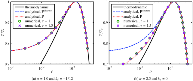
Figure 3: Comparisons of the coexistence curves given by the Maxwell construction (thermodynamic), the discrete form and continuum form pressure tensors ($\mathbf{P}^{\text{discrete}}$ and $\mathbf{P}$), and the numerical simulations ($\tau=1$ and $\tau=1.5$) for $\alpha=1.0$ and $\alpha=2.5$.

From the above analysis and comparisons, we can conclude that accurate pressure tensor can be definitely obtained in the continuum form when, and only when, the third-order isotropic term is considered, and the classical discrete form pressure tensor is accurate only when $k_{d}=-1/12$ ($\alpha=1$ or $\sigma_{e}=\sigma_{p}$). For the general equilibrium moment with $\alpha\neq 1$, the third-order isotropic term can be exploited to adjust the coexistence densities (mechanical stability condition) simply and directly (as indicated by Eq. (45) and illustrated by Fig. 3). However, this approach has a direct effect on the bulk viscosity and may cause numerical instability when $\alpha$ deviates strongly from the classical value $1.0$. Therefore, in next section, a consistent scheme for third-order additional term will be proposed to adjust the coexistence densities, as well as the surface tension simultaneously and independently.

6 Scheme for third-order additional term

6.1 LB model with additional term

In the framework of the present third-order analysis, a consistent scheme is proposed to introduce additional term into the recovered macroscopic equation, which can be used to independently adjust the coexistence densities (mechanical stability condition) and surface tension. The additional term is devised to be recovered at the third-order, just like the existing terms $\mathbf{R}_{\text{iso}}$ and $\mathbf{R}_{\text{aniso}}$, and thus it makes no difference to the Navier-Stokes level (second-order) macroscopic equation. To introduce such additional term, the collision step in the moment space (i.e., Eq. (2)) is changed to

$$\bar{\mathbf{m}}(\mathbf{x},t)=\mathbf{m}(\mathbf{x},t)-\mathbf{S}\left[\mathbf{m}(\mathbf{x},t)-\mathbf{m}^{\text{eq}}(\mathbf{x},t)\right]+\delta_{t}\left(\mathbf{I}-\dfrac{\mathbf{S}}{2}\right)\mathbf{F}_{m}(\mathbf{x},t)+\mathbf{SQ}_{m}(\mathbf{x},t),$$ (47)

where $\mathbf{Q}_{m}(\mathbf{x},t)$ is the discrete additional term in the moment space. Inspired by the idea of Li and Luo [41], $\mathbf{Q}_{m}(\mathbf{x},t)$ can be chosen in the following form

$$\mathbf{Q}_{m}=\Big{(}0,\;Q_{m1},\;Q_{m2},\;0,\;0,\;0,\;0,\;Q_{m7},\;Q_{m8}\Big{)}^{\text{T}}.$$ (48)

To determine $\mathbf{Q}_{m}$, systematic analysis is necessary and will be carried out in next section. The streaming step is described by Eq. (3). The equilibrium moment $\mathbf{m}^{\text{eq}}$, the discrete force term $\mathbf{F}_{m}$, and the macroscopic variables are still given by Eqs. (5), (6), and (7), respectively. Here, it is very interesting to note that the exact-difference-method (EDM) forcing scheme [47], which has attracted much attention in the pseudopotential LB community, can be reformulated in the form of Eq. (47), as presented in A.

6.2 Theoretical analysis

With the new collision step given by Eq. (47), the corresponding Taylor series expansion of the MRT LBE in the moment space becomes

$$(\mathbf{I}\partial_{t}+\mathbf{D})\mathbf{m}+\dfrac{\delta_{t}}{2}(\mathbf{I}\partial_{t}+\mathbf{D})^{2}\mathbf{m}+\dfrac{\delta_{t}^{2}}{6}(\mathbf{I}\partial_{t}+\mathbf{D})^{3}\mathbf{m}+O(\delta_{t}^{3})=-\dfrac{\mathbf{S}}{\delta_{t}}(\mathbf{m}-\mathbf{m}^{\text{eq}})+\left(\mathbf{I}-\dfrac{\mathbf{S}}{2}\right)\mathbf{F}_{m}+\dfrac{\mathbf{S}}{\delta_{t}}\mathbf{Q}_{m}.$$ (49)

In order to make the additional term recovered at the third-order ($\varepsilon^{3}$), $\mathbf{Q}_{m}$ is assumed to be at the order of $\varepsilon^{2}$ , i.e., $\mathbf{Q}_{m}=\varepsilon^{2}\mathbf{Q}_{m}^{(2)}$. Then, Eq. (49) can be rewritten in the consecutive orders of $\varepsilon$ as follows

$$\varepsilon^{0}:\;\mathbf{m}^{(0)}=\mathbf{m}^{\text{eq}},$$ (50a)

$$\varepsilon^{1}:\;(\mathbf{I}\partial_{t1}+\mathbf{D}_{1})\mathbf{m}^{(0)}-\mathbf{F}_{m}^{(1)}=-\dfrac{\mathbf{S}}{\delta_{t}}\left(\mathbf{m}^{(1)}+\dfrac{\delta_{t}}{2}\mathbf{F}_{m}^{(1)}\right),$$ (50b)

$$\varepsilon^{2}:\;\partial_{t2}\mathbf{m}^{(0)}+(\mathbf{I}\partial_{t1}+\mathbf{D}_{1})\mathbf{m}^{(1)}+\dfrac{\delta_{t}}{2}(\mathbf{I}\partial_{t1}+\mathbf{D}_{1})^{2}\mathbf{m}^{(0)}=-\dfrac{\mathbf{S}}{\delta_{t}}\mathbf{m}^{(2)}+\dfrac{\mathbf{S}}{\delta_{t}}\mathbf{Q}_{m}^{(2)},$$ (50c)

$$\varepsilon^{3}:\;\left(\begin{aligned} &\partial_{t3}\mathbf{m}^{(0)}+\partial_{t2}\mathbf{m}^{(1)}+(\mathbf{I}\partial_{t1}+\mathbf{D}_{1})\mathbf{m}^{(2)}+\delta_{t}(\mathbf{I}\partial_{t1}+\mathbf{D}_{1})\partial_{t2}\mathbf{m}^{(0)}+\\ &\dfrac{\delta_{t}}{2}(\mathbf{I}\partial_{t1}+\mathbf{D}_{1})^{2}\mathbf{m}^{(1)}+\dfrac{\delta_{t}^{2}}{6}(\mathbf{I}\partial_{t1}+\mathbf{D}_{1})^{3}\mathbf{m}^{(0)}\end{aligned}\right)=-\dfrac{\mathbf{S}}{\delta_{t}}\mathbf{m}^{(3)}.$$ (50d)

From Eq. (50), we can see that $\mathbf{Q}_{m}^{(2)}$ appears in the second-order ($\varepsilon^{2}$) equation and will have an effect on the following third-order ($\varepsilon^{3}$) equation. According to the second-order Chapman-Enskog analysis in Section 3, only the equations for the conserved moments ($m_{0}$, $m_{3}$, and $m_{5}$) in the second-order equation are involved to recover the Navier-Stokes level macroscopic equation. Therefore, further considering $Q_{m0}^{(2)}=Q_{m3}^{(2)}=Q_{m5}^{(2)}\equiv 0$ (see Eq. (48)), $\mathbf{Q}_{m}^{(2)}$ in Eq. (50c) truly makes no difference to the Navier-Stokes level macroscopic equation, i.e., Eq. (21) can still be recovered from Eqs. (50a), (50b), and (50c).

To identify the additional term introduced by $\mathbf{Q}_{m}$ at the third-order, a steady and stationary situation can be considered, as analyzed in Section 4. Then, Eq. (50) can be simplified as

$$\varepsilon^{0}:\;\mathbf{m}^{(0)}=\mathbf{m}^{\text{eq}},$$ (51a)

$$\varepsilon^{1}:\;\partial_{t1}\mathbf{m}^{(0)}+\mathbf{D}_{1}\mathbf{m}^{(0)}-\mathbf{F}_{m}^{(1)}=-\dfrac{\mathbf{S}}{\delta_{t}}\left(\mathbf{m}^{(1)}+\dfrac{\delta_{t}}{2}\mathbf{F}_{m}^{(1)}\right),$$ (51b)

$$\varepsilon^{2}:\;\partial_{t2}\mathbf{m}^{(0)}-\delta_{t}\mathbf{D}_{1}\left(\mathbf{S}^{-1}-\dfrac{\mathbf{I}}{2}\right)\left(\mathbf{D}_{1}\mathbf{m}^{(0)}-\mathbf{F}_{m}^{(1)}\right)=-\dfrac{\mathbf{S}}{\delta_{t}}\mathbf{m}^{(2)}+\dfrac{\mathbf{S}}{\delta_{t}}\mathbf{Q}_{m}^{(2)},$$ (51c)

$$\varepsilon^{3}:\;\partial_{t3}\mathbf{m}^{(0)}+\delta_{t}^{2}\left[\mathbf{D}_{1}\left(\mathbf{S}^{-1}-\dfrac{\mathbf{I}}{2}\right)\mathbf{D}_{1}\left(\mathbf{S}^{-1}-\dfrac{\mathbf{I}}{2}\right)\left(\mathbf{D}_{1}\mathbf{m}^{(0)}-\mathbf{F}_{m}^{(1)}\right)-\dfrac{1}{12}\mathbf{D}_{1}^{3}\mathbf{m}^{(0)}\right]+\mathbf{D}_{1}\mathbf{Q}_{m}^{(2)}=-\dfrac{\mathbf{S}}{\delta_{t}}\mathbf{m}^{(3)}.$$ (51d)

After the same processes performed in Section 4, the following third-order macroscopic equation can be recovered

$$\begin{cases}\partial_{t}\rho=0,\\ \partial_{t}(\rho\mathbf{u})=-\nabla(\tfrac{1}{3}\rho c^{2})+\mathbf{F}+\mathbf{R}_{\text{iso}}+\mathbf{R}_{\text{aniso}}+\mathbf{R}_{Q},\end{cases}$$ (52)

where $\mathbf{R}_{Q}$ is the third-order additional term introduced by $\mathbf{Q}_{m}$ that is expressed as

$$\mathbf{R}_{Q}=-c^{2}\left[\partial_{x}\left(\tfrac{1}{6}Q_{m1}+\tfrac{1}{2}Q_{m7}\right)+\partial_{y}Q_{m8},\;\partial_{x}Q_{m8}+\partial_{y}\left(\tfrac{1}{6}Q_{m1}-\tfrac{1}{2}Q_{m7}\right)\right]^{\text{T}}.$$ (53)

From Eq. (53), it can be seen that $Q_{m2}$ makes no difference to the third-order additional term.

With the consideration of the additional term $\mathbf{R}_{Q}$, the continuum form pressure tensor (see Eq. (38)) is redefined as

$$\nabla\cdot\mathbf{P}=\nabla(\tfrac{1}{3}\rho c^{2})-\mathbf{F}-\mathbf{R}_{\text{iso}}-\mathbf{R}_{Q}.$$ (54)

In order to independently adjust the mechanical stability condition (coexistence densities) and surface tension, we take

$$\mathbf{R}_{Q}=-\nabla\cdot\left[k_{1}G\delta_{x}^{4}\nabla\psi\nabla\psi+k_{2}G\delta_{x}^{4}(\nabla\psi\cdot\nabla\psi)\mathbf{I}\right],$$ (55)

and subsequently, we can finally obtain the continuum form pressure tensor as follows (see Section 5.2)

$$\begin{split}\mathbf{P}=\Bigg{(}\dfrac{\rho c^{2}}{3}+\dfrac{G\delta_{x}^{2}}{2}\psi^{2}&+\dfrac{G\delta_{x}^{4}}{6}\left[\left(a_{3}-6k_{d}b_{2}+6k_{2}\right)\nabla\psi\cdot\nabla\psi+\left(a_{4}-6k_{d}b_{2}\right)\psi\nabla\cdot\nabla\psi\right]\Bigg{)}\mathbf{I}\\ &+\dfrac{G\delta_{x}^{4}}{6}\left[\left(a_{1}-6k_{d}b_{1}+6k_{1}\right)\nabla\psi\nabla\psi+\left(a_{2}-6k_{d}b_{1}\right)\psi\nabla\nabla\psi\right]+O(\nabla^{4}).\end{split}$$ (56)

Here, $k_{1}$ and $k_{2}$ are the adjustable parameters. As compared with Eq. (43), the introduction of $\mathbf{R}_{Q}$ given by Eq. (55) only changes the coefficients before the terms $\nabla\psi\nabla\psi$ and $(\nabla\psi\cdot\nabla\psi)\mathbf{I}$ in Eq. (56). Comparing Eq. (55) with Eq. (53), we can choose

$$\begin{split}Q_{m1}&=3\left(k_{1}+2k_{2}\right)G\delta_{x}^{4}\dfrac{\partial_{x}\psi\partial_{x}\psi+\partial_{y}\psi\partial_{y}\psi}{c^{2}},\\ Q_{m7}&=k_{1}G\delta_{x}^{4}\dfrac{\partial_{x}\psi\partial_{x}\psi-\partial_{y}\psi\partial_{y}\psi}{c^{2}},\\ Q_{m8}&=k_{1}G\delta_{x}^{4}\dfrac{\partial_{x}\psi\partial_{y}\psi}{c^{2}}.\end{split}$$ (57)

Eq. (57) is in the continuum form. In real application, the gradient of $\psi$, $\nabla\psi=(\partial_{x}\psi,\,\partial_{y}\psi)^{\text{T}}$, needs to be calculated by an isotropic central scheme (ICS) as follows

$$\nabla\psi\approx\dfrac{1}{\delta_{x}^{2}}\sum\limits_{i=1}^{8}\omega(|\mathbf{e}_{i}\delta_{t}|^{2})\psi(\mathbf{x}+\mathbf{e}_{i}\delta_{t})\mathbf{e}_{i}\delta_{t}=-\dfrac{\mathbf{F}}{G\delta_{x}^{2}\psi},$$ (58)

where the nearest-neighbor interaction force (i.e., Eq. (8)), as a finite-difference gradient operator, is utilized to simplify the ICS. Therefore, $Q_{m1}$, $Q_{m7}$, and $Q_{m8}$ can be further written in a discrete form as

$$\begin{split}Q_{m1}&=3\left(k_{1}+2k_{2}\right)\dfrac{|\mathbf{F}|^{2}}{G\psi^{2}c^{2}},\\ Q_{m7}&=k_{1}\dfrac{F_{x}^{2}-F_{y}^{2}}{G\psi^{2}c^{2}},\\ Q_{m8}&=k_{1}\dfrac{F_{x}F_{y}}{G\psi^{2}c^{2}}.\end{split}$$ (59)

In the Chapman-Enskog analysis, $\mathbf{F}$ is at the order of $\varepsilon$. According to Eq. (59), $\mathbf{Q}_{m}$ is at the order of $\varepsilon^{2}$, which is consistent with the aforementioned assumption, and $\mathbf{R}_{Q}=-\nabla\cdot\big{(}k_{1}G^{-1}\psi^{-2}\mathbf{FF}+k_{2}G^{-1}\psi^{-2}|\mathbf{F}|^{2}\mathbf{I}\big{)}$ is at the order of $\varepsilon^{3}$, which is consistent with the fact that $\mathbf{R}_{Q}$ is recovered at the third-order. This consistency is the reason why we call the present scheme for additional term a consistent scheme. However, in previous works [12, 39, 38], similar third-order terms, like $\nabla\cdot(h\mathbf{FF})$ ($h$ is a coefficient), are inconsistently recovered and analyzed at the second-order. Note that $Q_{m2}$ in $\mathbf{Q}_{m}$ is still undetermined. Based on the third-order analysis, $Q_{m2}$ can be chosen arbitrarily, and it is set as $Q_{m2}=-Q_{m1}$ in the present work.

To show the adjustments of the mechanical stability condition and surface tension by $\mathbf{R}_{Q}$, a steady-state one-dimensional flat interface along $y$ direction is considered again. The normal pressure $P_{n}$ and tangential pressure $P_{\tau}$ given by Eq. (56) are

$$P_{n}=P_{xx}=\dfrac{\rho c^{2}}{3}+\dfrac{G\delta_{x}^{2}}{2}\psi^{2}+\dfrac{G\delta_{x}^{4}}{6}\left[-\dfrac{1+12k_{d}-12k_{1}-12k_{2}}{2}\left(\dfrac{d\psi}{dx}\right)^{2}+\left(1-6k_{d}\right)\psi\dfrac{d^{2}\psi}{dx^{2}}\right],$$ (60a)

$$P_{\tau}=P_{yy}=\dfrac{\rho c^{2}}{3}+\dfrac{G\delta_{x}^{2}}{2}\psi^{2}+\dfrac{G\delta_{x}^{4}}{6}\left[\left(a_{3}-6k_{d}b_{2}+6k_{2}\right)\left(\dfrac{d\psi}{dx}\right)^{2}+\left(a_{4}-6k_{d}b_{2}\right)\psi\dfrac{d^{2}\psi}{dx^{2}}\right],$$ (60b)

where Eqs. (40) and (42) have been used for the simplifications. Then, the mechanical stability condition and surface tension can be obtained as

$$\int_{\rho_{g}}^{\rho_{l}}\left(p_{0}-\dfrac{\rho c^{2}}{3}-\dfrac{G\delta_{x}^{2}}{2}\psi^{2}\right)\dfrac{\psi^{\prime}}{\psi^{1+\epsilon}}d\rho=0\enskip\text{with}\enskip\epsilon=\dfrac{1+12k_{d}-12k_{1}-12k_{2}}{1-6k_{d}},$$ (61)

$$\sigma=\int_{-\infty}^{+\infty}\left(P_{n}-P_{\tau}\right)dx=-\dfrac{G\delta_{x}^{4}}{6}\left(1-6k_{1}\right)\int_{\rho_{g}}^{\rho_{l}}\psi^{\prime 2}\sqrt{\varrho}\,d\rho,$$ (62)

where $\psi^{\prime}=d\psi/d\rho$ and $\varrho=(d\rho/dx)^{2}$. From Eqs. (61) and (62), we can clearly see that the mechanical stability condition and surface tension can be adjusted by $k_{1}+k_{2}$ and $k_{1}$, respectively.

6.3 Numerical validations

Numerical simulations are then carried out to validate the above theoretical analysis of the present scheme for third-order additional term. The basic simulation parameters are chosen the same as in Section 5. The rest simulation parameters are set as follows: $\alpha=1$, $s_{0}=s_{j}=1$, $s_{p}=s_{e}=s_{\varepsilon}=1/\tau$, and $s_{q}=1/[0.5+{\it\Lambda}/(s_{p}^{-1}-0.5)]$ with ${\it\Lambda}\equiv 1/12$. Then, there have $k_{d}=-1/12$ and $\epsilon=-8(k_{1}+k_{2})$. Considering $\tau$ makes invisible difference to the numerical results, it is chosen as $\tau=1.5$ here. Note that, though $\alpha=1$ is chosen which means $\mathbf{R}_{\text{aniso}}=\mathbf{0}$, it is still recommended to set ${\it\Lambda}\equiv 1/12$. This is because that when the surface tension is adjusted by $k_{1}$, anisotropic term introduced by $\mathbf{Q}_{m}$ at the fifth-order may be amplified and then needs to be considered. By setting ${\it\Lambda}\equiv 1/12$, this anisotropic term can be eliminated, just like $\mathbf{R}_{\text{aniso}}$. A fifth-order heuristic analysis on this point is given in B. What is more, setting ${\it\Lambda}\equiv 1/12$ can help reduce the spurious current based on our numerical tests.

To validate the adjustment of the mechanical stability condition (coexistence densities), the one-dimensional flat interface along $y$ direction is simulated on a $N_{x}\times N_{y}=1024\times 8$ lattice. Periodic boundary conditions are applied in both directions and the initial density and velocity fields are still given by Eq. (46). The coexistence curves for the cases $\epsilon=1$ and $\epsilon=2$ are shown in Fig. 4(a) and Fig. 4(b), respectively. It can be seen that the numerical results are always in good agreement with the analytical results predicted by the mechanical stability condition (i.e., Eq. (61)), which validates the free adjustment of the mechanical stability condition (coexistence densities) by the present scheme and also verifies the theoretical analysis in Section 6.2. What is more, Fig. 4 also shows that, as long as $\epsilon=-8(k_{1}+k_{2})$ keeps unvaried, the coexistence densities do not vary with $k_{1}$. Thus, the surface tension can be independently adjusted by varying the value of $k_{1}$ while fixing the value of $\epsilon$. Note that, by properly setting the value of $\epsilon$, the coexistence densities can be adjusted to approximate the thermodynamic results in real application [12].

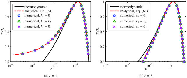
Figure 4: Comparisons of the coexistence curves given by the Maxwell construction (thermodynamic), the mechanical stability condition (Eq. (61)), and the numerical simulations ($k_{1}=0$, $k_{1}=k_{2}$, and $k_{2}=0$).

To clearly show the adjustment of the surface tension, numerical simulations of stationary droplets with different radii are carried out on a $N_{x}\times N_{y}=256\times 265$ lattice with periodic boundary conditions in both directions. The temperature is fixed at $T=0.9T_{c}$, and the initial density and velocity fields are given by Eq. (32) except that the radius $r_{0}$ varies from $32\delta_{x}$ to $96\delta_{x}$. The surface tension is numerically determined through the Laplace’s law, i.e., $\delta p=p_{\text{in}}-p_{\text{out}}=\sigma/r$. Here, $p_{\text{in}}$ and $p_{\text{out}}$ denote the pressure inside and outside of the droplet, and $r$ is the final radius of the droplet. Fig. 5 gives the numerical results of $\delta p$ versus $1/r$ for the cases $\epsilon=1$ and $\epsilon=2$ with $1-6k_{1}$ varying from $0.1$ to $2.0$. It clearly shows that the numerical results are in good agreement with the linear fits denoted by the dashed lines, which validates the Laplace’s law. The slopes of the linear fits are equal to the surface tensions, which are listed in Table 1. As it can be seen, when $1-6k_{1}$ varies from $0.1$ to $2.0$, the surface tension $\sigma$ varies from $1.5814\times 10^{-4}$ to $2.6174\times 10^{-3}$ for $\epsilon=1$ and from $1.4828\times 10^{-4}$ to $2.4574\times 10^{-3}$ for $\epsilon=2$. Note that, when the surface tension is too small, it does not vary linearly with $1-6k_{1}$ as indicated by Eq. (62), probably because that the influence of the truncated higher-order terms on the surface tension is relatively strong under this condition. What is more, when the surface tension is adjusted by $1-6k_{1}$, the gas and liquid densities outside and inside the droplet vary slightly though $\epsilon$ keeps unvaried, which can be seen from Table 1 for $r_{0}=64\delta_{x}$ as an example. This phenomenon is caused by the intrinsic property of the EOS, i.e., both the gas and liquid phases are compressible to some degree.

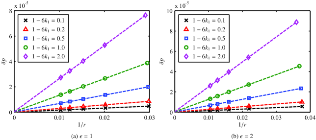
Figure 5: Variations of the pressure difference inside and outside of the droplet $\delta p$ with the reciprocal of the droplet radius $1/r$ for different $1-6k_{1}$. The dashed lines are the corresponding linear fits to the symbols.

Table 1: Surface tensions ($\sigma$) determined through the Laplace’s law for different $1-6k_{1}$, together with the gas and liquid densities ($\rho_{g}$ and $\rho_{l}$) given for $r_{0}=64\delta_{x}$.

	$1-6k_{1}$		$\epsilon=1$						$\epsilon=2$
			$\sigma$		$\rho_{g}(r_{0}=64\delta_{x})$		$\rho_{l}(r_{0}=64\delta_{x})$		$\sigma$		$\rho_{g}(r_{0}=64\delta_{x})$		$\rho_{l}(r_{0}=64\delta_{x})$
	0.1		$1.5814\times 10^{-4}$		$4.3726\times 10^{-2}$		$2.4743\times 10^{-1}$		$1.4828\times 10^{-4}$		$4.7530\times 10^{-2}$		$2.4883\times 10^{-1}$
	0.2		$2.8370\times 10^{-4}$		$4.3708\times 10^{-2}$		$2.4745\times 10^{-1}$		$2.6579\times 10^{-4}$		$4.7515\times 10^{-2}$		$2.4884\times 10^{-1}$
	0.5		$6.6303\times 10^{-4}$		$4.3655\times 10^{-2}$		$2.4750\times 10^{-1}$		$6.2125\times 10^{-4}$		$4.7469\times 10^{-2}$		$2.4890\times 10^{-1}$
	1.0		$1.3038\times 10^{-3}$		$4.3566\times 10^{-2}$		$2.4758\times 10^{-1}$		$1.2219\times 10^{-3}$		$4.7392\times 10^{-2}$		$2.4898\times 10^{-1}$
	2.0		$2.6174\times 10^{-3}$		$4.3388\times 10^{-2}$		$2.4776\times 10^{-1}$		$2.4574\times 10^{-3}$		$4.7239\times 10^{-2}$		$2.4916\times 10^{-1}$

7 Conclusions

In this paper, we have performed a third-order Chapman-Enskog analysis of the MRT pseudopotential LB model for multiphase flow for the first time. The third-order leading terms on the interaction force are successfully identified in the recovered macroscopic equation, and then some theoretical aspects, which are still unclear or inconsistent in the pseudopotential LB model, are discussed and clarified. Firstly, the isotropic property of the LBE is investigated specifically. Numerical tests show that the third-order anisotropic term recovered by the LBE needs to be eliminated for multiphase flow, which means the isotropy of the LBE should be third-order at least in the pseudopotential LB model. As indicated by the present third-order analysis, this can be realized by adopting the classical equilibrium moment or setting the so-called “magic” parameter to $1/12$. Then, the determination of the pressure tensor, which is of crucial importance for multiphase flow, is analyzed. It is shown that when and only when the third-order isotropic term recovered by the LBE is considered, accurate continuum form pressure tensor can be obtained from the recovered macroscopic equation. By contrast, as also demonstrated by numerical tests, the classical discrete form pressure tensor is accurate only when the third-order isotropic term is a specific one. Finally, in the framework of the present third-order analysis, a consistent scheme for third-order additional term is proposed. By the present scheme, the coexistence densities (mechanical stability condition) and surface tension can be adjusted independently, which have been validated by the subsequent numerical tests. In summary, by performing a third-order Chapman-Enskog analysis, the theoretical foundations for the pseudopotential LB model are further consolidated in this work. Simultaneously, the application of the pseudopotential LB model can be extended by the present consistent scheme for third-order additional term.

Appendix A Reformulation of the EDM forcing scheme

The single-relaxation-time (SRT) LBE for the EDM forcing scheme is written as [47]

$$f_{i}(\mathbf{x}+\mathbf{e}_{i}\delta_{t},t+\delta_{t})=f_{i}(\mathbf{x},t)-\dfrac{1}{\tau}\left[f_{i}(\mathbf{x},t)-f_{i}^{\text{eq}}(\rho,\mathbf{v})\right]+\left[f_{i}^{\text{eq}}(\rho,\mathbf{v}+\delta\mathbf{v})-f_{i}^{\text{eq}}(\rho,\mathbf{v})\right],$$ (63)

where $\rho\mathbf{v}=\sum\nolimits_{i=0}^{8}\mathbf{e}_{i}f_{i}$, $\delta\mathbf{v}=\delta_{t}\mathbf{F}/\rho$, and $f_{i}^{\text{eq}}(\rho,\mathbf{v})$ is the equilibrium distribution function. The macroscopic density $\rho$ and velocity $\mathbf{u}$ are defined as

$$\rho=\sum\limits_{i=0}^{8}f_{i},\qquad\rho\mathbf{u}=\sum\limits_{i=0}^{8}\mathbf{e}_{i}f_{i}+\dfrac{\delta_{t}}{2}\mathbf{F}=\rho\left(\mathbf{v}+\dfrac{\delta\mathbf{v}}{2}\right).$$ (64)

The MRT LBE for the EDM forcing scheme can be easily extended from Eq. (63). The corresponding collision step is

$$\bar{\mathbf{m}}(\mathbf{x},t)=\mathbf{m}(\mathbf{x},t)-\mathbf{S}\left[\mathbf{m}(\mathbf{x},t)-\mathbf{m}^{\text{eq}}(\rho,\mathbf{v})\right]+\left[\mathbf{m}^{\text{eq}}(\rho,\mathbf{v}+\delta\mathbf{v})-\mathbf{m}^{\text{eq}}(\rho,\mathbf{v})\right],$$ (65)

where $\mathbf{m}^{\text{eq}}(\rho,\mathbf{v})=\mathbf{M}\big{[}f_{0}^{\text{eq}}(\rho,\mathbf{v}),\,\cdots,\,f_{8}^{\text{eq}}(\rho,\mathbf{v})\big{]}^{\text{T}}$ is the equilibrium moment that can be given as

$$\mathbf{m}^{\text{eq}}(\rho,\mathbf{v})=\left(\rho,\;-2\rho+3\rho\dfrac{|\mathbf{v}|^{2}}{c^{2}},\;\alpha\rho-3\rho\dfrac{|\mathbf{v}|^{2}}{c^{2}},\;\rho\dfrac{v_{x}}{c},\;-\rho\dfrac{v_{x}}{c},\;\rho\dfrac{v_{y}}{c},\;-\rho\dfrac{v_{y}}{c},\;\rho\dfrac{v_{x}^{2}-v_{y}^{2}}{c^{2}},\;\rho\dfrac{v_{x}v_{y}}{c^{2}}\right)^{\text{T}}.$$ (66)

Substituting the relations $\mathbf{u}=\mathbf{v}+\delta\mathbf{v}/2$ and $\delta\mathbf{v}=\delta_{t}\mathbf{F}/\rho$ into Eq. (65), Eq. (65) can be reformulated as

$$\begin{split}\bar{\mathbf{m}}(\mathbf{x},t)&=\mathbf{m}(\mathbf{x},t)-\mathbf{S}\left[\mathbf{m}(\mathbf{x},t)-\mathbf{m}^{\text{eq}}(\rho,\mathbf{u}-\tfrac{\delta_{t}}{2\rho}\mathbf{F})\right]+\left[\mathbf{m}^{\text{eq}}(\rho,\mathbf{u}+\tfrac{\delta_{t}}{2\rho}\mathbf{F})-\mathbf{m}^{\text{eq}}(\rho,\mathbf{u}-\tfrac{\delta_{t}}{2\rho}\mathbf{F})\right]\\ &=\mathbf{m}(\mathbf{x},t)-\mathbf{S}\left[\mathbf{m}(\mathbf{x},t)-\mathbf{m}^{\text{eq}}(\rho,\mathbf{u})\right]+\left(\begin{aligned} &\left(\mathbf{I}-\tfrac{\mathbf{S}}{2}\right)\left[\mathbf{m}^{\text{eq}}(\rho,\mathbf{u}+\tfrac{\delta_{t}}{2\rho}\mathbf{F})-\mathbf{m}^{\text{eq}}(\rho,\mathbf{u}-\tfrac{\delta_{t}}{2\rho}\mathbf{F})\right]+\\ &\tfrac{\mathbf{S}}{2}\left[\mathbf{m}^{\text{eq}}(\rho,\mathbf{u}+\tfrac{\delta_{t}}{2\rho}\mathbf{F})+\mathbf{m}^{\text{eq}}(\rho,\mathbf{u}-\tfrac{\delta_{t}}{2\rho}\mathbf{F})-2\mathbf{m}^{\text{eq}}(\rho,\mathbf{u})\right]\end{aligned}\right)\\ &=\mathbf{m}(\mathbf{x},t)-\mathbf{S}\left[\mathbf{m}(\mathbf{x},t)-\mathbf{m}^{\text{eq}}(\rho,\mathbf{u})\right]+\delta_{t}\left(\mathbf{I}-\dfrac{\mathbf{S}}{2}\right)\mathbf{F}_{m}(\mathbf{x},t)+\mathbf{S}\mathbf{Q}_{m}^{\text{EDM}}(\mathbf{x},t),\end{split}$$ (67)

where

$$\begin{split}\mathbf{F}_{m}(\mathbf{x},t)&=\dfrac{1}{\delta_{t}}\left[\mathbf{m}^{\text{eq}}(\rho,\mathbf{u}+\tfrac{\delta_{t}}{2\rho}\mathbf{F})-\mathbf{m}^{\text{eq}}(\rho,\mathbf{u}-\tfrac{\delta_{t}}{2\rho}\mathbf{F})\right]\\ &=\left(0,\;6\dfrac{\mathbf{F}\cdot\mathbf{u}}{c^{2}},\;-6\dfrac{\mathbf{F}\cdot\mathbf{u}}{c^{2}},\;\dfrac{F_{x}}{c},\;-\dfrac{F_{x}}{c},\;\dfrac{F_{y}}{c},\;-\dfrac{F_{y}}{c},\;2\dfrac{F_{x}u_{x}-F_{y}u_{y}}{c^{2}},\;\dfrac{F_{x}u_{y}+F_{y}u_{x}}{c^{2}}\right)^{\text{T}},\end{split}$$ (68a)

$$\begin{split}\mathbf{Q}_{m}^{\text{EDM}}(\mathbf{x},t)&=\dfrac{1}{2}\left[\mathbf{m}^{\text{eq}}(\rho,\mathbf{u}+\tfrac{\delta_{t}}{2\rho}\mathbf{F})+\mathbf{m}^{\text{eq}}(\rho,\mathbf{u}-\tfrac{\delta_{t}}{2\rho}\mathbf{F})-2\mathbf{m}^{\text{eq}}(\rho,\mathbf{u})\right]\\ &=\left(0,\;\dfrac{3}{4}\dfrac{\delta_{x}^{2}|\mathbf{F}|^{2}}{\rho c^{4}},\;-\dfrac{3}{4}\dfrac{\delta_{x}^{2}|\mathbf{F}|^{2}}{\rho c^{4}},\;0,\;0,\;0,\;0,\;\dfrac{1}{4}\dfrac{\delta_{x}^{2}(F_{x}^{2}-F_{y}^{2})}{\rho c^{4}},\;\dfrac{1}{4}\dfrac{\delta_{x}^{2}F_{x}F_{y}}{\rho c^{4}}\right)^{\text{T}}.\end{split}$$ (68b)

Obviously, Eqs. (67) and (47) are the same except the different coefficients in the discrete additional term $\mathbf{Q}_{m}$. Based on the above analysis, the nature of the EDM forcing scheme is revealed from a new perspective.

Appendix B Fifth-order heuristic analysis on $\mathbf{Q}_{m}$

Performing the Taylor series expansion of the streaming step (i.e., Eq. (3)) to fifth-order, and correspondingly the Taylor series expansion of the MRT LBE in the moment space becomes

$$\left(\begin{aligned} &(\mathbf{I}\partial_{t}+\mathbf{D})\mathbf{m}+\dfrac{\delta_{t}}{2}(\mathbf{I}\partial_{t}+\mathbf{D})^{2}\mathbf{m}+\dfrac{\delta_{t}^{2}}{6}(\mathbf{I}\partial_{t}+\mathbf{D})^{3}\mathbf{m}+\\ &\dfrac{\delta_{t}^{3}}{24}(\mathbf{I}\partial_{t}+\mathbf{D})^{4}\mathbf{m}+\dfrac{\delta_{t}^{4}}{120}(\mathbf{I}\partial_{t}+\mathbf{D})^{5}\mathbf{m}+O(\delta_{t}^{5})\end{aligned}\right)=-\dfrac{\mathbf{S}}{\delta_{t}}(\mathbf{m}-\mathbf{m}^{\text{eq}})+\left(\mathbf{I}-\dfrac{\mathbf{S}}{2}\right)\mathbf{F}_{m}+\dfrac{\mathbf{S}}{\delta_{t}}\mathbf{Q}_{m},$$ (69)

which can be rewritten in the consecutive orders of $\varepsilon$ as

$$\varepsilon^{0}:\;\mathbf{m}^{(0)}=\mathbf{m}^{\text{eq}},$$ (70a)

$$\varepsilon^{1}:\;(\mathbf{I}\partial_{t1}+\mathbf{D}_{1})\mathbf{m}^{(0)}-\mathbf{F}_{m}^{(1)}=-\dfrac{\mathbf{S}}{\delta_{t}}\left(\mathbf{m}^{(1)}+\dfrac{\delta_{t}}{2}\mathbf{F}_{m}^{(1)}\right),$$ (70b)

$$\varepsilon^{2}:\;\partial_{t2}\mathbf{m}^{(0)}+(\mathbf{I}\partial_{t1}+\mathbf{D}_{1})\mathbf{m}^{(1)}+\dfrac{\delta_{t}}{2}(\mathbf{I}\partial_{t1}+\mathbf{D}_{1})^{2}\mathbf{m}^{(0)}=-\dfrac{\mathbf{S}}{\delta_{t}}\mathbf{m}^{(2)}+\dfrac{\mathbf{S}}{\delta_{t}}\mathbf{Q}_{m}^{(2)},$$ (70c)

$$\varepsilon^{3}:\;\left(\begin{aligned} &\partial_{t3}\mathbf{m}^{(0)}+\partial_{t2}\mathbf{m}^{(1)}+(\mathbf{I}\partial_{t1}+\mathbf{D}_{1})\mathbf{m}^{(2)}+\delta_{t}(\mathbf{I}\partial_{t1}+\mathbf{D}_{1})\partial_{t2}\mathbf{m}^{(0)}+\\ &\dfrac{\delta_{t}}{2}(\mathbf{I}\partial_{t1}+\mathbf{D}_{1})^{2}\mathbf{m}^{(1)}+\dfrac{\delta_{t}^{2}}{6}(\mathbf{I}\partial_{t1}+\mathbf{D}_{1})^{3}\mathbf{m}^{(0)}\end{aligned}\right)=-\dfrac{\mathbf{S}}{\delta_{t}}\mathbf{m}^{(3)},$$ (70d)

$$\varepsilon^{4}:\;\left(\begin{aligned} &\partial_{t4}\mathbf{m}^{(0)}+\partial_{t3}\mathbf{m}^{(1)}+\partial_{t2}\mathbf{m}^{(2)}+(\mathbf{I}\partial_{t1}+\mathbf{D}_{1})\mathbf{m}^{(3)}+\delta_{t}(\mathbf{I}\partial_{t1}+\mathbf{D}_{1})\partial_{t3}\mathbf{m}^{(0)}+\dfrac{\delta_{t}}{2}\partial_{t2}^{2}\mathbf{m}^{(0)}+\\ &\delta_{t}(\mathbf{I}\partial_{t1}+\mathbf{D}_{1})\partial_{t2}\mathbf{m}^{(1)}+\dfrac{\delta_{t}}{2}(\mathbf{I}\partial_{t1}+\mathbf{D}_{1})^{2}\mathbf{m}^{(2)}+\dfrac{\delta_{t}^{2}}{2}(\mathbf{I}\partial_{t1}+\mathbf{D}_{1})^{2}\partial_{t2}\mathbf{m}^{(0)}+\\ &\dfrac{\delta_{t}^{2}}{6}(\mathbf{I}\partial_{t1}+\mathbf{D}_{1})^{3}\mathbf{m}^{(1)}+\dfrac{\delta_{t}^{3}}{24}(\mathbf{I}\partial_{t1}+\mathbf{D}_{1})^{4}\mathbf{m}^{(0)}\end{aligned}\right)=-\dfrac{\mathbf{S}}{\delta_{t}}\mathbf{m}^{(4)},$$ (70e)

$$\varepsilon^{5}:\;\left(\begin{aligned} &\partial_{t5}\mathbf{m}^{(0)}+\partial_{t4}\mathbf{m}^{(1)}+\partial_{t3}\mathbf{m}^{(2)}+\partial_{t2}\mathbf{m}^{(3)}+(\mathbf{I}\partial_{t1}+\mathbf{D}_{1})\mathbf{m}^{(4)}+\delta_{t}\partial_{t2}\partial_{t3}\mathbf{m}^{(0)}+\dfrac{\delta_{t}}{2}\partial_{t2}^{2}\mathbf{m}^{(1)}+\\ &\delta_{t}(\mathbf{I}\partial_{t1}+\mathbf{D}_{1})\partial_{t4}\mathbf{m}^{(0)}+\delta_{t}(\mathbf{I}\partial_{t1}+\mathbf{D}_{1})\partial_{t3}\mathbf{m}^{(1)}+\delta_{t}(\mathbf{I}\partial_{t1}+\mathbf{D}_{1})\partial_{t2}\mathbf{m}^{(2)}+\\ &\dfrac{\delta_{t}}{2}(\mathbf{I}\partial_{t1}+\mathbf{D}_{1})^{2}\mathbf{m}^{(3)}+\dfrac{\delta_{t}^{2}}{2}(\mathbf{I}\partial_{t1}+\mathbf{D}_{1})^{2}\partial_{t3}\mathbf{m}^{(0)}+\dfrac{\delta_{t}^{2}}{2}(\mathbf{I}\partial_{t1}+\mathbf{D}_{1})\partial_{t2}^{2}\mathbf{m}^{(0)}+\\ &\dfrac{\delta_{t}^{2}}{2}(\mathbf{I}\partial_{t1}+\mathbf{D}_{1})^{2}\partial_{t2}\mathbf{m}^{(1)}+\dfrac{\delta_{t}^{2}}{6}(\mathbf{I}\partial_{t1}+\mathbf{D}_{1})^{3}\mathbf{m}^{(2)}+\dfrac{\delta_{t}^{3}}{6}(\mathbf{I}\partial_{t1}+\mathbf{D}_{1})^{3}\partial_{t2}\mathbf{m}^{(0)}+\\ &\dfrac{\delta_{t}^{3}}{24}(\mathbf{I}\partial_{t1}+\mathbf{D}_{1})^{4}\mathbf{m}^{(1)}+\dfrac{\delta_{t}^{4}}{120}(\mathbf{I}\partial_{t1}+\mathbf{D}_{1})^{5}\mathbf{m}^{(0)}\end{aligned}\right)=-\dfrac{\mathbf{S}}{\delta_{t}}\mathbf{m}^{(5)}.$$ (70f)

Similarly, a steady and stationary situation is considered, and the lower-order equations are used to simplify the higher-order equations. Finally, we can obtain

$$\varepsilon^{0}:\;\mathbf{m}^{(0)}=\mathbf{m}^{\text{eq}},$$ (71a)

$$\varepsilon^{1}:\;\partial_{t1}\mathbf{m}^{(0)}+\mathbf{D}_{1}\mathbf{m}^{(0)}-\mathbf{F}_{m}^{(1)}=-\dfrac{\mathbf{S}}{\delta_{t}}\left(\mathbf{m}^{(1)}+\dfrac{\delta_{t}}{2}\mathbf{F}_{m}^{(1)}\right),$$ (71b)

$$\varepsilon^{2}:\;\partial_{t2}\mathbf{m}^{(0)}-\delta_{t}\mathbf{D}_{1}\left(\mathbf{S}^{-1}-\tfrac{\mathbf{I}}{2}\right)\left(\mathbf{D}_{1}\mathbf{m}^{(0)}-\mathbf{F}_{m}^{(1)}\right)=-\dfrac{\mathbf{S}}{\delta_{t}}\mathbf{m}^{(2)}+\dfrac{\mathbf{S}}{\delta_{t}}\mathbf{Q}_{m}^{(2)},$$ (71c)

$$\varepsilon^{3}:\;\partial_{t3}\mathbf{m}^{(0)}+\left(\begin{aligned} &\delta_{t}^{2}\left[\mathbf{D}_{1}\left(\mathbf{S}^{-1}-\tfrac{\mathbf{I}}{2}\right)\mathbf{D}_{1}\left(\mathbf{S}^{-1}-\tfrac{\mathbf{I}}{2}\right)\left(\mathbf{D}_{1}\mathbf{m}^{(0)}-\mathbf{F}_{m}^{(1)}\right)-\tfrac{1}{12}\mathbf{D}_{1}^{3}\mathbf{m}^{(0)}\right]+\\ &\mathbf{D}_{1}\mathbf{Q}_{m}^{(2)}\end{aligned}\right)=-\dfrac{\mathbf{S}}{\delta_{t}}\mathbf{m}^{(3)},$$ (71d)

$$\varepsilon^{4}:\;\partial_{t4}\mathbf{m}^{(0)}-\left(\begin{aligned} &\delta_{t}^{3}\left[\begin{aligned} &\mathbf{D}_{1}\left(\mathbf{S}^{-1}-\tfrac{\mathbf{I}}{2}\right)\mathbf{D}_{1}\left(\mathbf{S}^{-1}-\tfrac{\mathbf{I}}{2}\right)\mathbf{D}_{1}\left(\mathbf{S}^{-1}-\tfrac{\mathbf{I}}{2}\right)\left(\mathbf{D}_{1}\mathbf{m}^{(0)}-\mathbf{F}_{m}^{(1)}\right)+\\ &\tfrac{1}{12}\mathbf{D}_{1}^{3}\left(\mathbf{S}^{-1}-\tfrac{\mathbf{I}}{2}\right)\left(\mathbf{D}_{1}\mathbf{m}^{(0)}-\mathbf{F}_{m}^{(1)}\right)+\tfrac{1}{12}\mathbf{D}_{1}\left(\mathbf{S}^{-1}-\tfrac{\mathbf{I}}{2}\right)\mathbf{D}_{1}^{3}\mathbf{m}^{(0)}\end{aligned}\right]+\\ &\delta_{t}\mathbf{D}_{1}\left(\mathbf{S}^{-1}-\tfrac{\mathbf{I}}{2}\right)\mathbf{D}_{1}\mathbf{Q}_{m}^{(2)}\end{aligned}\right)=-\dfrac{\mathbf{S}}{\delta_{t}}\mathbf{m}^{(4)},$$ (71e)

$$\varepsilon^{5}:\;\partial_{t5}\mathbf{m}^{(0)}+\left(\begin{aligned} &\delta_{t}^{4}\left[\begin{aligned} &\mathbf{D}_{1}\left(\mathbf{S}^{-1}-\tfrac{\mathbf{I}}{2}\right)\mathbf{D}_{1}\left(\mathbf{S}^{-1}-\tfrac{\mathbf{I}}{2}\right)\mathbf{D}_{1}\left(\mathbf{S}^{-1}-\tfrac{\mathbf{I}}{2}\right)\mathbf{D}_{1}\left(\mathbf{S}^{-1}-\tfrac{\mathbf{I}}{2}\right)\left(\mathbf{D}_{1}\mathbf{m}^{(0)}-\mathbf{F}_{m}^{(1)}\right)-\\ &\tfrac{1}{12}\mathbf{D}_{1}^{3}\left(\mathbf{S}^{-1}-\tfrac{\mathbf{I}}{2}\right)\mathbf{D}_{1}\left(\mathbf{S}^{-1}-\tfrac{\mathbf{I}}{2}\right)\left(\mathbf{D}_{1}\mathbf{m}^{(0)}-\mathbf{F}_{m}^{(1)}\right)-\\ &\tfrac{1}{12}\mathbf{D}_{1}\left(\mathbf{S}^{-1}-\tfrac{\mathbf{I}}{2}\right)\mathbf{D}_{1}^{3}\left(\mathbf{S}^{-1}-\tfrac{\mathbf{I}}{2}\right)\left(\mathbf{D}_{1}\mathbf{m}^{(0)}-\mathbf{F}_{m}^{(1)}\right)-\\ &\tfrac{1}{12}\mathbf{D}_{1}\left(\mathbf{S}^{-1}-\tfrac{\mathbf{I}}{2}\right)\mathbf{D}_{1}\left(\mathbf{S}^{-1}-\tfrac{\mathbf{I}}{2}\right)\mathbf{D}_{1}^{3}\mathbf{m}^{(0)}+\tfrac{1}{120}\mathbf{D}_{1}^{5}\mathbf{m}^{(0)}\end{aligned}\right]+\\ &\delta_{t}^{2}\left[\mathbf{D}_{1}\left(\mathbf{S}^{-1}-\tfrac{\mathbf{I}}{2}\right)\mathbf{D}_{1}\left(\mathbf{S}^{-1}-\tfrac{\mathbf{I}}{2}\right)\mathbf{D}_{1}\mathbf{Q}_{m}^{(2)}-\tfrac{1}{12}\mathbf{D}_{1}^{3}\mathbf{Q}_{m}^{(2)}\right]\end{aligned}\right)=-\dfrac{\mathbf{S}}{\delta_{t}}\mathbf{m}^{(5)}.$$ (71f)

From Eq. (71), we can see that the differential operator before $\mathbf{Q}_{m}^{(2)}$ at the order of $\varepsilon^{n+2}$ is the same as that before $\mathbf{m}^{(0)}$ at the order of $\varepsilon^{n}$. For example, the differential operator before $\mathbf{Q}_{m}^{(2)}$ at the fifth-order (see Eq. (71f)) is $\mathbf{D}_{1}(\mathbf{S}^{-1}-\mathbf{I}/2)\mathbf{D}_{1}(\mathbf{S}^{-1}-\mathbf{I}/2)\mathbf{D}_{1}-\mathbf{D}_{1}^{3}/12$, which is identical to the differential operator before $\mathbf{m}^{(0)}$ at the third-order (see Eq. (71d)). From the third-order analysis in Section 4, it is found that anisotropic term will appear at the third-order if $\mathbf{m}^{(0)}=\mathbf{m}^{\text{eq}}$ is not chosen specifically. Considering the form of $\mathbf{Q}_{m}$ given by Eqs. (48) and (59) does not coincide with the form of $\mathbf{m}^{\text{eq}}$ no matter how $Q_{m2}$ is chosen, anisotropic term about $\mathbf{Q}_{m}$ will appear at the fifth-order. Generally, the effect of this fifth-order anisotropic term can be neglected. However, when the surface tension is adjusted by $k_{1}$, this anisotropic term may be amplified synchronously, and then needs to be considered. By setting the “magic” parameter ${\it\Lambda}\equiv 1/12$, this fifth-order anisotropic term can be eliminated just as the third-order anisotropic term $\mathbf{R}_{\text{aniso}}$, because of the same differential operator before $\mathbf{Q}_{m}^{(2)}$ in Eq. (71f) and $\mathbf{m}^{(0)}$ in Eq. (71d).

References

References

- [1] S. van der Graaf, T. Nisisako, C. G. P. H. Schroën, R. G. M. van der Sman, R. M. Boom, Lattice Boltzmann simulations of droplet formation in a T-shaped microchannel, Langmuir 22 (2006) 4144–4152.
- [2] G. Hazi, A. Markus, On the bubble departure diameter and release frequency based on numerical simulation results, International Journal of Heat and Mass Transfer 52 (2009) 1472–1480.
- [3] R. Ledesma-Aguilar, D. Vella, J. M. Yeomans, Lattice-Boltzmann simulations of droplet evaporation, Soft Matter 10 (2014) 8267–8275.
- [4] Q. Li, K. H. Luo, Q. J. Kang, Y. L. He, Q. Chen, Q. Liu, Lattice Boltzmann methods for multiphase flow and phase-change heat transfer, Progress in Energy and Combustion Science 52 (2016) 62–105.
- [5] A. K. Gunstensen, D. H. Rothman, S. Zaleski, G. Zanetti, Lattice Boltzmann model of immiscible fluids, Physical Review A 43 (1991) 4320–4327.
- [6] D. Grunau, S. Chen, K. Eggert, A lattice Boltzmann model for multiphase fluid flows, Physics of Fluids A 5 (1993) 2557–2562.
- [7] M. Latva-Kokko, D. H. Rothman, Diffusion properties of gradient-based lattice Boltzmann models of immiscible fluids, Physical Review E 71 (2005) 056702.
- [8] H. Liu, A. J. Valocchi, Q. Kang, Three-dimensional lattice Boltzmann model for immiscible two-phase flow simulations, Physical Review E 85 (2012) 046309.
- [9] X. Shan, H. Chen, Lattice Boltzmann model for simulating flows with multiple phases and components, Physical Review E 47 (1993) 1815–1819.
- [10] X. Shan, H. Chen, Simulation of nonideal gases and liquid-gas phase transitions by the lattice Boltzmann equation, Physical Review E 49 (1994) 2941–2948.
- [11] M. Sbragaglia, R. Benzi, L. Biferale, S. Succi, K. Sugiyama, F. Toschi, Generalized lattice Boltzmann method with multirange pseudopotential, Physical Review E 75 (2007) 026702.
- [12] Q. Li, K. H. Luo, X. J. Li, Forcing scheme in pseudopotential lattice Boltzmann model for multiphase flows, Physical Review E 86 (2012) 016709.
- [13] S. Khajepor, J. Wen, B. Chen, Multipseudopotential interaction: A solution for thermodynamic inconsistency in pseudopotential lattice Boltzmann models, Physical Review E 91 (2015) 023301.
- [14] M. R. Swift, W. R. Osborn, J. M. Yeomans, Lattice Boltzmann simulation of nonideal fluids, Physical Review Letters 75 (1995) 830–833.
- [15] M. R. Swift, E. Orlandini, W. R. Osborn, J. M. Yeomans, Lattice Boltzmann simulations of liquid-gas and binary fluid systems, Physical Review E 54 (1996) 5041–5052.
- [16] T. Inamuro, N. Konishi, F. Ogino, A Galilean invariant model of the lattice Boltzmann method for multiphase fluid flows using free-energy approach, Computer Physics Communications 129 (2000) 32–45.
- [17] C. M. Pooley, K. Furtado, Eliminating spurious velocities in the free-energy lattice Boltzmann method, Physical Review E 77 (2008) 046702.
- [18] L. S. Luo, Unified theory of lattice Boltzmann models for nonideal gases, Physical Review Letters 81 (1998) 1618–1621.
- [19] X. He, G. D. Doolen, Thermodynamic foundations of kinetic theory and lattice Boltzmann models for multiphase flows, Journal of Statistical Physics 107 (2002) 309–328.
- [20] M. E. McCracken, J. Abraham, Multiple-relaxation-time lattice-Boltzmann model for multiphase flow, Physical Review E 71 (2005) 036701.
- [21] E. S. Kikkinides, A. G. Yiotis, M. E. Kainourgiakis, A. K. Stubos, Thermodynamic consistency of liquid-gas lattice Boltzmann methods: Interfacial property issues, Physical Review E 78 (2008) 036702.
- [22] X. Shan, Analysis and reduction of the spurious current in a class of multiphase lattice Boltzmann models, Physical Review E 73 (2006) 047701.
- [23] S. Chibbaro, G. Falcucci, G. Chiatti, H. Chen, X. Shan, S. Succi, Lattice Boltzmann models for nonideal fluids with arrested phase-separation, Physical Review E 77 (2008) 036705.
- [24] L. Clime, D. Brassard, T. Veres, Numerical modeling of electrowetting transport processes for digital microfluidics, Microfluidics and Nanofluidics 8 (2009) 599–608.
- [25] Z. Yu, L. S. Fan, An interaction potential based lattice Boltzmann method with adaptive mesh refinement (AMR) for two-phase flow simulation, Journal of Computational Physics 228 (2009) 6456–6478.
- [26] S. Varagnolo, D. Ferraro, P. Fantinel, M. Pierno, G. Mistura, G. Amati, L. Biferale, M. Sbragaglia, Stick-slip sliding of water drops on chemically heterogeneous surfaces, Physical Review Letters 111 (2013) 066101.
- [27] Q. Li, Q. J. Kang, M. M. Francois, A. J. Hu, Lattice Boltzmann modeling of self-propelled Leidenfrost droplets on ratchet surfaces, Soft Matter 12 (2016) 302–312.
- [28] D. Sun, M. Zhu, J. Wang, B. Sun, Lattice Boltzmann modeling of bubble formation and dendritic growth in solidification of binary alloys, International Journal of Heat and Mass Transfer 94 (2016) 474–487.
- [29] A. J. Wagner, C. M. Pooley, Interface width and bulk stability: Requirements for the simulation of deeply quenched liquid-gas systems, Physical Review E 76 (2007) 045702.
- [30] H. Huang, M. Krafczyk, X. Lu, Forcing term in single-phase and Shan-Chen-type multiphase lattice Boltzmann models, Physical Review E 84 (2011) 046710.
- [31] Q. Li, K. H. Luo, X. J. Li, Lattice Boltzmann modeling of multiphase flows at large density ratio with an improved pseudopotential model, Physical Review E 87 (2013) 053301.
- [32] Z. Guo, C. Zheng, B. Shi, Force imbalance in lattice Boltzmann equation for two-phase flows, Physical Review E 83 (2011) 036707.
- [33] Y. Xiong, Z. Guo, Effects of density and force discretizations on spurious velocities in lattice Boltzmann equation for two-phase flows, Journal of Physics A: Mathematical and Theoretical 47 (2014) 195502.
- [34] A. J. Wagner, The origin of spurious velocities in lattice Boltzmann, International Journal of Modern Physics B 17 (2003) 193–196.
- [35] Z. Yu, L. S. Fan, Multirelaxation-time interaction-potential-based lattice Boltzmann model for two-phase flow, Physical Review E 82 (2010) 046708.
- [36] A. J. Wagner, Thermodynamic consistency of liquid-gas lattice Boltzmann simulations, Physical Review E 74 (2006) 056703.
- [37] K. Sun, T. Wang, M. Jia, G. Xiao, Evaluation of force implementation in pseudopotential-based multiphase lattice Boltzmann models, Physica A: Statistical Mechanics and its Applications 391 (2012) 3895–3907.
- [38] A. Zarghami, N. Looije, H. Van den Akker, Assessment of interaction potential in simulating nonisothermal multiphase systems by means of lattice Boltzmann modeling, Physical Review E 92 (2015) 023307.
- [39] A. Hu, L. Li, R. Uddin, Force method in a pseudo-potential lattice Boltzmann model, Journal of Computational Physics 294 (2015) 78–89.
- [40] D. Lycett-Brown, K. H. Luo, Improved forcing scheme in pseudopotential lattice Boltzmann methods for multiphase flow at arbitrarily high density ratios, Physical Review E 91 (2015) 023305.
- [41] Q. Li, K. H. Luo, Achieving tunable surface tension in the pseudopotential lattice Boltzmann modeling of multiphase flows, Physical Review E 88 (2013) 053307.
- [42] P. Lallemand, L. S. Luo, Theory of the lattice Boltzmann method: Dispersion, dissipation, isotropy, Galilean invariance, and stability, Physical Review E 61 (2000) 6546–6562.
- [43] Z. Guo, C. Zheng, Analysis of lattice Boltzmann equation for microscale gas flows: Relaxation times, boundary conditions and the Knudsen layer, International Journal of Computational Fluid Dynamics 22 (2008) 465–473.
- [44] Z. Guo, C. Zheng, B. Shi, Discrete lattice effects on the forcing term in the lattice Boltzmann method, Physical Review E 65 (2002) 046308.
- [45] X. Shan, Pressure tensor calculation in a class of nonideal gas lattice Boltzmann models, Physical Review E 77 (2008) 066702.
- [46] P. Yuan, L. Schaefer, Equations of state in a lattice Boltzmann model, Physics of fluids 18 (2006) 042101.
- [47] A. L. Kupershtokh, D. A. Medvedev, D. I. Karpov, On equations of state in a lattice Boltzmann method, Computers & Mathematics with Applications 58 (2009) 965–974.
- [48] Z. Guo, C. Zheng, B. Shi, T. S. Zhao, Thermal lattice Boltzmann equation for low Mach number flows: Decoupling model, Physical Review E 75 (2007) 036704.
- [49] M. Sbragaglia, D. Belardinelli, Interaction pressure tensor for a class of multicomponent lattice Boltzmann models, Physical Review E 88 (2013) 013306.