Thermodynamics of the collapse transition of the all-backbone peptide Gly₁₅

Abstract

Simulations show Gly₁₅, a polypeptide lacking any side-chains, can collapse in water. We assess the hydration thermodynamics in this collapse by calculating the hydration free energy at each of the end points of the reaction coordinate, here the end-to-end distance ($r$) in the chain. To examine the role of the various conformations for a given $r$, we study the conditional distribution, $P(R_{g}|r)$, of the radius of gyration for a given value of $r$. $P(R_{g}|r)$ is found to vary more gently compared to the corresponding variation in the excess hydration free energy. Using this insight within a multistate generalization of the potential distribution theorem, we calculate a reasonable upper bound for the hydration free energy of the peptide for a given $r$. On this basis we find that peptide hydration greatly favors the expanded state of the chain, despite primitive hydrophobic effects favoring chain collapse. The net free energy of collapse is seen to be a delicate balance between opposing intra-peptide and hydration effects, with intra-peptide contributions favoring collapse by a small margin. The favorable intra-peptide interactions are primarily electrostatic in origin, and found to arise primarily from interaction between C=O dipoles, hydrogen bonding interaction between C=O and N-H groups, and favorable interaction between N-H dipoles.

The concept of hydrophobic hydration, the tendency of apolar solutes to disfavor the aqueous phase, informs nearly all aspects of biomolecular self-assembly and is commonly accepted as providing the driving force for proteins to fold Kauzmann (1959); Chandler (2005); Dill (1990); Dill and MacCallum (2012). However, this rationalization cannot explain recent experimental Teufel et al. (2011) and simulational Tran et al. (2008); Hu et al. (2010a) observations that oligoglycine, only mildly hydrophobic by some accounts Cornette et al. (1987); Wilce et al. (1995), also collapses into a non-specific structure in liquid water.

Experimental studies on the collapse of (Gly)_n and the closely related (GlySer)_n polypeptides have attributed the collapse to the formation of intramolecular hydrogen bonds Möglich et al. (2006); Teufel et al. (2011). However, an earlier simulation study has suggested that collapse is unlikely to be driven solely by intramolecular hydrogen bonding Tran et al. (2008). They have instead postulated that the unfavorable cost of creating a cavity to accommodate the peptide drives the collapse, a picture that is synonymous with hydrophobicity driven collapse. More recent work has implicated the charge ordering and the favorable correlation between the CO groups of the peptide as an important determinant in oligoglycine collapse Karandur et al. (2014, 2015). A rigorous analysis of hydration effects in folding of Gly₁₅ has not yet been presented.

Here we explore the hydration thermodynamics of Gly₁₅ collapse using the recently developed regularization approach to free energy calculations Weber et al. (2011); Weber and Asthagiri (2012). This approach makes possible the facile calculation of free energies of hydration of polypetides and proteins in all-atom simulations. Importantly, this approach provides direct quantification of the hydrophilic and hydrophobic contributions to hydration Tomar et al. (2014, 2016). We complement these studies with evaluation of the excess enthalpy and entropy of hydration as well Tomar et al. (2014, 2016). Our results show that in contrast to the usual paradigm of water aiding folding by decreasing the mutual solubility of the peptide units comprising the polypeptide chain, hydration in fact drives unfolding in this peptide; importantly, intra-peptide van der Waals and electrostatic interactions are critical in driving Gly₁₅ to collapse. Some of the favorable electrostatic interactions are clearly attributable to the formation of hydrogen bonds, as was suspected in the experimental studies Möglich et al. (2006); Teufel et al. (2011).

I Methods

Gly₁₅ was constructed with capped ends and solvated by a box containing 13358 CHARMM-modified TIP3P Jorgensen et al. (1983); Neria et al. (1996) water molecules. (The equilibrated system is a cube of edge length $\approx 73.5$ Å. The starting equilibrated configuration was kindly provided by Karandur and Pettitt Karandur et al. (2015), who had simulated the system for over 100 ns at a temperature of 300 K and a pressure of 1 atm. using, respectively, a Langevin thermostat and a Langevin barostat Feller et al. (1995).) We maintained the simulation parameters as in the Karandur-Pettitt study. Specifically, the barostat piston period was 100 fs and the decay time was 50 fs. The decay constant of the thermostat was 4 ps^-1. The SHAKE algorithm was used to constrain the geometry of water molecules and fix the bond between hydrogens and parent heavy atoms. Lennard-Jones interactions were terminated at 12.00 Å by smoothly switching to zero starting at 10.0 Å. Electrostatic interactions were treated with the particle mesh Ewald method with a grid spacing of 1.0 Å. In contrast to the Karandur-Pettitt study, here we use a 2.0 fs timestep. In vacuo calculations for peptide provided the vacuum reference. These in vacuo simulations lasted at least 25 ns with a 1 fs timestep. The decay constant of the thermostat was 10 ps^-1.

To calculate the potential of mean force (PMF), $W(r)$, where the order parameter $r$ is the distance between the terminal carbon atoms of the Gly₁₅ peptide, we first obtained one frame each with $r\in(30,40)$ Å (domain L40), $r\in(25,35)$ Å (domain L35), and $r\in(20,30)$ Å (domain L30) from the earlier simulations by Karandur and Pettitt Karandur et al. (2015). Then the PMFs in the respective domains were obtained using the adaptive-bias force (ABF) technique Darve et al. (2008); Hénin et al. (2010). Briefly, in the ABF approach, the order parameter is binned in windows of width 0.1 Å and using these counts initial biasing forces are estimated that encourage a uniform sampling of the order parameter in the chosen domain. As the simulation progresses, the distribution of $r$ and hence also the biasing forces are updated. At convergence, the biasing force should cancel the force due to the underlying free energy surface (the quantity of interest), thus allowing the calculation of $W(r)$.

For each domain, ABF simulations spanned 26 ns. The first 16 ns was set aside for equilibration, during which time we monitored the evolution of the biasing forces. Then the gradient of $W(r)$ obtained at the end of 18, 20, 22, 24, and 26 ns was averaged. The forces from the overlapping segments in L30 and L35 were averaged. The L30-L35 average and forces from L40 were then averaged to construct the gradient of $W(r)$ in the entire domain $r\in[20,40]$ Å. The gradient was then numerically integrated (a trapezoidal rule suffices) to obtained $W(r)$ from $r=20.1$ Å to $r=39.9$ Å. (For the in vacuo ABF simulation, we follow a similar procedure with gradients obtained at the end of 10, 15, 20, and 25 ns.) The potential energy of the peptide (in the solvent) as a function of $r$ was obtained from the last 4 ns of the ABF trajectory and sorted and binned in windows of width 0.1 Å along $r$. For the potential energy calculation, we used structures only from L40 and L30 simulations.

The calculation of $\mu^{\rm ex}$ and its entropic $Ts^{\rm ex}$ and enthalpic $h^{\rm ex}$ follows earlier work Tomar et al. (2013, 2014, 2016). For completeness, the calculation approach is briefly described in the Appendix.

II Results

II.1 Free energy of chain compaction

Figure 1 shows the potential of mean force (PMF) between the terminal carbon atoms of the Gly₁₅.

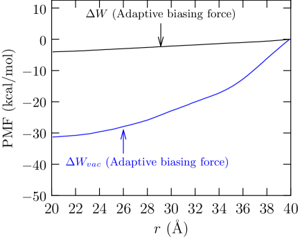
Figure 1: Left panel: PMF, $\Delta W(r)$, relative to $r=40$ Å for Gly₁₅ folding in the domain $r\in[20,40]$ Å. PMF obtained from ABF is shown as solid black line. Right panel: The change in the internal energy $\Delta E$ (red line) and its electrostatic (blue) and van der Waals (grey) contributions for the solvated peptide. The light red shading indicates the $1\sigma$ standard error of the mean. The contributions from dihedral and angle terms of the forcefield are negligible on the scale of the graph.

As $r$ decreases from 40 Å to 20 Å, the radius of gyration of the peptide changes from about 13 Å to about 6 Å, indicating that the polypeptide adopts a compact configuration as $r$ decreases. Figure 1 shows that chain compaction is favored by a free energy change of approximately $-4$ kcal/mol. Observe that there is an intrinsic drive for the peptide chain to collapse, as is seen in the potential of mean force for chain compaction obtained in the absence of the solvent ($\Delta W_{vac}$) and as can also be inferred from the large intra-peptide energy change accompanying chain compaction (Fig. 1, right panel).

II.2 Analysis of intra-peptide interactions

Given their role in organized structures such as the $\alpha$-helix and the $b$-sheet, it is natural to suspect that hydrogen bonds would contribute to the favorable intra-peptide electrostatic interaction, as has been suggested in earlier experimental studies Möglich et al. (2006); Teufel et al. (2011). It is standard practice, for example see Ref. 6, to identify hydrogen bonds on the basis of a geometric criterion. However, to obtain a better understanding of the role of hydrogen bonds in the electrostatic contribution, which is of first interest here, it is also necessary to evaluate their energetic contribution. To this end, we analyzed hydrogen bonding contributions using both geometric and energetic criteria.

First for all the sampled configurations (in $r\in[20,40]$ Å), we calculated the number of hydrogen bonds based on the distance $r_{c}$ between the carbonyl oxygen for residue $i$ and the amide nitrogen (N) at $j$ and the angle $\theta_{c}$ between the N-H (amide proton) vector and the N-O vector. (For assessing hydrogen bonds, $i$ and $j$ differ by at least 2 residues.) For a hydrogen bond pair satisfying the defined cutoffs, we find the pair interaction energy between the [CO]_i group and the $[{\rm HNC_{\alpha}(H_{\alpha})_{2}}]_{j}$ group. (Our choice of interacting groups is based on the fact that within the CHARMM forcefield, the CO group is neutral as is the $[{\rm HNC_{\alpha}(H_{\alpha})_{2}}]$ group, but the bare NH group is not.) Figure 2 collects the results of this analysis for two commonly used cutoffs.

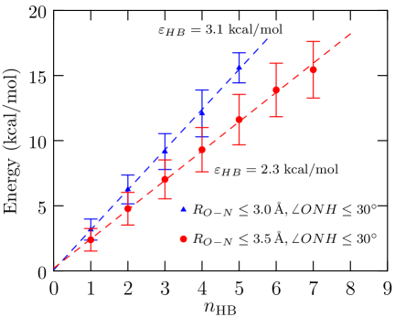
Figure 2: Analysis of hydrogen bonding strength for hydrogen bonds defined according to various geometric criteria. $\varepsilon_{HB}$ is the slope of the line and defines the average contribution of the single hydrogen bond based on the specified geometric criterion. The role of the end-caps, which can also hydrogen bond, is ignored. Standard error of the mean is shown at $1\sigma$.

Figure 2 shows that the net interaction energy energy is linear in the number of hydrogen bond for both the defined cutoffs (Fig. 2). Thus we can conclude that for the given forcefield, a hydrogen bond based on $r_{c}\leq 3.0$ Å and $\theta_{c}\leq 30^{\circ}$ contributes on average 3.1 kcal/mol favorably to the net binding strength. Likewise, a hydrogen bond based on $r_{c}\leq 3.5$ Å and $\theta_{c}\leq 30^{\circ}$ contributes on average 2.3 kcal/mol to the net binding strength; it should be clear, however, that this average includes the effect of the stronger hydrogen bonds that occur at the $3.1$ kcal/mol energy scale.

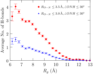
Figure S2: Average number of hydrogen bonds as a function of the radius of gyration $R_{g}$ and for various distance and angle criteria. The $R_{g}$ range is divided into 25 bins and configurations sorted into the appropriate bins. The mean number of hydrogen bonds from configurations in a bin and the associated standard error is then obtained using standard relations.

Figure 3 shows that the average number of hydrogen bonds increases as $r$ (and hence also $R_{g}$, Fig. S2) decreases, as has also been suggested experimentally Möglich et al. (2006); Teufel et al. (2011).

Figure 3: Average number of hydrogen bonds as a function of the order parameter $r$ for various distance and angle criteria. (The role of the end-caps, which can also hydrogen bond, is ignored.) For clarity, standard error at $2\sigma$ is shown as a shaded background only for $R_{O-N}\leq 3.5\,{\rm{\AA}},\angle ONH\leq 30^{\circ}$.

On average about 3 hydrogen bonds form upon collapse for the criterion $R_{ON}\leq 3.5$ Å and $\angle ONH\leq 30^{\circ}$. Based on the analysis in Fig. 2, we can infer than one of these is a H-bond contributing about 3.1 kcal/mol to the binding energy and the remaining two contribute about 1.9 kcal/mol (on average) to the binding energy.

Figure 4 compares the contribution from hydrogen bonds as well as due to interaction between CO-CO dipoles and NH-NH dipoles.

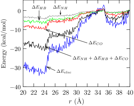
Figure 4: Analysis of contributions to the electrostatic contribution to the internal energy change. Only energetic contribution from hydrogen bonds satisfying $r_{c}\leq 3.5$ Å and $\theta_{c}\leq 30^{\circ}$ is shown. The contribution from CO_i-CO_j ($j\geq i+2$) pairs and NH_i-NH_j ($j\geq i+2$) pairs are also indicated. For interactions involving NH, we always consider the neutral $[{\rm HNC_{\alpha}(H_{\alpha})_{2}}]$ group. The role of the end-caps in H-bonding, CO-CO, and NH-NH interactions is ignored.

The results reveal that correlations between CO-groups play a larger role in the net electrostatic energy change than hydrogen bonds (based on $r_{c}\leq 3.5$ Å and $\theta_{c}\leq 30^{\circ}$, $\varepsilon_{HB}=2.3$ kcal/mol). Our identification of the importance of CO-CO interactions is consistent with what has been reported earlier by Karandur et al.  Karandur et al. (2014, 2015). However, in variance with their conclusion, we find that $\Delta E_{HB}$ also makes a significant contribution to the net electrostatic energy change. In particular, we find that $\Delta E_{HB}$ is about 63% of $\Delta E_{CO}$. In a similar vein, we find that correlations between NH groups also contributes favorably to the change in electrostatic energy. The sum of CO-CO, H-bonding, and NH-NH interactions is about 66% of the net electrostatic change. For simplicity we have not included the interactions involving the terminal caps, which can participate in all the three categories noted in Fig. 4. Further, in comparing with the molecular dynamics data (Fig. 4), we have ignored short range interaction involving partial charges that are not readily classifiable into one of the three defined categories noted in Fig. 4. These contributions that have been left out contribute the rest of the change in $\Delta E_{elec}$.

Summarizing the results of our analysis on intra-peptide interactions, we find that correlations between CO-groups and hydrogen bonds are two of the most important contributions to the favorable change in $\Delta E_{elec}$. The identified importance of hydrogen bonds is also in good agreement with expectations based on experiments Möglich et al. (2006); Teufel et al. (2011).

II.3 Role of hydration

We next consider the analysis of hydration effects. To parse the effect of hydration, we write

$$\Delta W=\Delta W_{vac}+\Delta W_{ss}\,,$$ (1)

where $\Delta W_{ss}$ accounts for all the hydration effects. Here $\Delta W_{ss}=\mu^{\rm ex}(r=20.1)-\mu^{\rm ex}(r=39.9)$, where $\mu^{\rm ex}(r)$ is the hydration free energy of the polypeptide with the constraint that the end-to-end distance is $r$. To estimate $\mu^{\rm ex}(r)$, we first classify the ensemble of conformations satisfying the constraint $r$ by the radius of gyration $R_{g}$. For a given $r$, denoting the excess chemical potential of a specific conformation $R_{g}$ by $\mu^{\rm ex}(R_{g}|r)$, the multistate generalization Pratt and Asthagiri (2007); Beck et al. (2006); Merchant and Asthagiri (2009); Dixit et al. (2009) of the chemical potential $\mu^{\rm ex}(r)$ gives

$$\beta\mu^{\rm ex}(r)=\ln\int_{R_{g}}e^{\beta\mu^{\rm ex}(R_{g}|r)}P(R_{g}|r)dR_{g}\,,$$ (2)

where the integration is over all the conformations (classified according to $R_{g}$) that satisfy the constraint of fixed $r$, and $\beta=1/k_{\rm B}T$, with $k_{\rm B}$ the Boltzmann constant and $T$ the temperature. $P(R_{g}|r)dR_{g}$ is probability of finding a conformation in the range $[R_{g},R_{g}+dR_{g}]$ given the constraint $r$.

Constructing $\mu^{\rm ex}(r)$ by calculating $\mu^{\rm ex}(R_{g}|r)$ for an ensemble of configurations is a daunting task, but much progress can be made using Eq. 2 and some physically realistic assumptions. First we note that hydration free energy calculations for several different conformations of Gly₁₅ shows that $\mu^{\rm ex}$ for a given conformation is negative (Fig. 5).

Figure 5: Hydration free energy values for several Gly₁₅ conformations for $R_{g}$ values of interest in the present study. The linear fit is solely to indicate that on average $\mu^{\rm ex}$ decreases with increasing $R_{g}$, i.e. as more of the chain is exposed to the solvent.

This negative $\mu^{\rm ex}$ is also consistent with explicit hydration free energy calculations on shorter polyglycines Tomar et al. (2013, 2014) and is as expected based on hydration free energy calculations of another homogeneous peptides of varying chain lengths (up to about 10), for example, see 27; 28; 29; 30; 31; 16.

Since $\mu^{\rm ex}(R_{g}|r)<0$, it is clear that $\mu^{\rm ex}(r)$ must be bounded from above by the least negative and from below by the most negative hydration free energy. Further since $\mu^{\rm ex}(R_{g}|r)$ decreases with increasing $R_{g}$, i.e. with increasing solvent exposure of the backbone, we can infer that for a given $r$, the hydration free energy $\mu^{\rm ex}(R_{g}|r)$ for the most collapsed conformation is expected to be least negative. Denoting the most collapsed conformation by $R^{*}_{g}$, we thus expect $[\mu^{\rm ex}(R_{g}|r)-\mu^{\rm ex}(R^{*}_{g}|r)]\leq 0$ and thus

$$\beta\mu^{\rm ex}(r) = \beta\mu^{\rm ex}(R^{*}_{g}|r)+\ln\int_{R_{g}}e^{\beta[\mu^{\rm ex}(R_{g}|r)-\mu^{\rm ex}(R^{*}_{g}|r)]}P(R_{g}|r)dR_{g}$$ (3)

$$\leq \beta\mu^{\rm ex}(R^{*}_{g}|r)\,.$$

For using Eq. 3, we first obtained two structures satisfying $r=39.9$ Å and $r=20.1$ Å, respectively, from the ABF trajectory. (We find a structure that is within 0.05 Å of the target distance and then adjust $r$.) Subsequently, these peptide configurations were centered and rotated such that the end-to-end vector is along the principal diagonal of the simulation cell. With the terminal carbon atoms fixed in space, we sampled conformations of the peptide from 2 ns of production.

Analysis of the distribution of $R_{g}$ for $r=20.1$ Å and $39.9$ Å, shows that $P(R_{g}^{*}|r)\approx e^{-2}$ relative to the most probable $\bar{R}_{g}$, i.e. $-\ln[P(R^{*}_{g}|r)/P(\bar{R}_{g}|r)]\approx 2\,{\rm k_{\rm B}T}$ (Fig. 6).

Figure 6: Probability distribution of $R_{g}$ values for the specified end-to-end distance. For $r=20.1$ Å, the $R_{g}$ of the most collapsed conformation is 5.5 Å and for $r=39.9$ Å, the $R_{g}$ of the most collapsed conformation is 10.8 Å. These $R_{g}$ values fall slightly to the left of the leftmost point shown in the plot.

But for the same increase in $R_{g}$, about 1 Å, the hydration free energy decreases by $O(17\,{\rm k_{\rm B}T})$ (Fig. 5). Because of the exponential dependence of the free energy on $[\mu^{\rm ex}(R_{g}|r)-\mu^{\rm ex}(R^{*}_{g}|r)]<0$ which decreases sharply relative to the growth in $P(R_{g}|r)$, we expect the upper bound to itself be a fair approximation to the required free energy. (See also Ref. 26 for a similar argument in the context of ion hydration.) Thus, we expect that the hydration contribution in Eq. 1 can be approximated as

$$\Delta W_{ss} = \mu^{\rm ex}[r=20.1~{}{\rm{\AA}}]-\mu^{\rm ex}[r=39.9~{}{\rm{\AA}}]$$ (4)

$$\approx \mu^{\rm ex}(R^{*}_{g}|r=20.1~{}{\rm{\AA}})-\mu^{\rm ex}(R^{*}_{g}|r=39.9~{}{\rm{\AA}})$$

For the $(R^{*}_{g}|r=20.1)$ and $(R^{*}_{g}|r=39.9)$ structures, we find the hydration free energy, $\mu^{\rm ex}$, using the regularization approach to hydration free energies Weber et al. (2011); Weber and Asthagiri (2012); Tomar et al. (2013, 2014) (Appendix A), a technique that is based on the extensively documented quasichemical organization of the potential distribution theorem Beck et al. (2006); Pratt and Asthagiri (2007). As before Tomar et al. (2014, 2016), we also obtained the entropic ($s^{\rm ex}$) and enthalpic ($h^{\rm ex}$) decomposition of $\mu^{\rm ex}$ (Appendix A).

Table 1 collects the results of the hydration analysis and it is clear that the calculated value of the free energy of collapse is in reasonable accord with the value obtained using the ABF procedure (Fig. 1).

Table 1: Hydration and intra-peptide interaction contributions in the collapse of Gly₁₅ from $r=39.9$ Å to $r=20.1$ Å. $\Delta W_{ss}$ is based on Eq. 4. $\Delta W({\rm calc.})=\Delta W_{ss}+W_{vac}$ is the value of the free energy of collapse using the calculated hydration free energy; $\Delta W$ (ABF) is the corresponding value from Fig. 1.

Quantity	(kcal/mol)
$\Delta W_{vac}$ (ABF)	$-31.3$
$\Delta W_{ss}$	$25.5\pm 2$
$\Delta W$ (calc.)	$-5.8\pm 2$
$\Delta W$ (ABF)	$-4.0$

Analyzing $\Delta W_{ss}$ shows that the packing contribution, a measure of primitive hydrophobic effectsPratt and Pohorille (1992); Pratt (2002), does favor chain compaction, as is expected (Fig. 7).

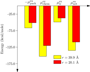
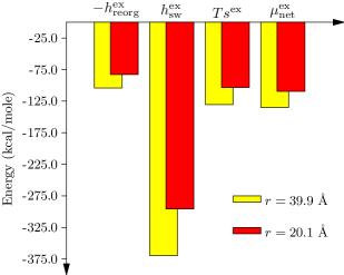
Figure 7: Left panel: The hydration free energy and its components based on the quasichemical decompostion Beck et al. (2006); Pratt and Asthagiri (2007); Weber et al. (2011); Weber and Asthagiri (2012); Tomar et al. (2013, 2014). (See Appendix.) The packing contribution measures the free energy to create a cavity to accommodate the peptide Tomar et al. (2014, 2016); it is the domain that is excluded to the solvent centers and is uniquely defined for the given forcefield. The chemistry contribution captures the role of solute attractive interactions with solvent in the first hydration shell, here defined to be the surface at a distance of 5 Å away from nearest heavy atom in the solute. The long-range contribution is the free energy of interaction between the peptide and the solvent when solvent is excluded from the first hydration layer. Right panel: Decomposition of the hydration free energy change into enthalpic and entropic contributions. The enthalpy of hydration is further separated into a solvent reorganization and solute-solvent interaction parts.

But this packing contribution is approximately balanced by the long-range contributions that favor chain unfolding. Importantly, the chemistry contribution reflecting the role of favorable solute interactions with the solvent in the first hydration shell is nearly twice the magnitude of the packing contribution and favors chain unfolding. Thus hydrophilic effects overwhelm hydrophobic effects to shift the balance to the unfolded state.

Mirroring the packing contribution, the energetic cost to reorganize the solvent around a cavity ($h^{\rm ex}_{reorg}$) favors chain compaction, as does the entropy of hydration. But favorable solute-water interactions reflected in $h^{\rm ex}_{sw}$ greatly favor chain expansion. This observation suggests that the backbone must play a substantial role in protein folding, consistent with several recent studies Rose et al. (2006); Bolen and Rose (2008); Auton et al. (2011).

III Conclusions

We find that the collapse of Gly₁₅ is driven by intra-molecular interactions, which are primarily electrostatic in origin. The basis for this electrostatic drive is found mostly in favorable CO-CO interactions, hydrogen bonding interactions between CO and NH groups, and also interaction between amide group (NH) dipoles. Favorable solute-solvent interaction dominates the hydration thermodynamics and opposes the collapse of Gly₁₅, despite packing (or primitive hydrophobic) effects favoring chain compaction. The net balance between intramolecular interactions and hydration is such that intramolecular contributions win by a small margin and drive the collapse of the peptide. Thus liquid water is both a good solvent for the hydration of the peptide unit Hu et al. (2010b); Tomar et al. (2013), but also a poor solvent from the perspective of folding, as the hydration effects lose in comparison to intra-peptide interactions. Our work suggests that the hydration of the peptide backbone is likely an important determinant in the solution thermodynamics of intrinsically disordered peptides, an aspect that needs to be investigated further. The observed feature of hydration opposing collapse driven by favorable intramolecular interactions is also expected to be relevant to protein folding and assembly.

IV Appendix

S.I Methods

The free energy of hydration, $\mu^{\rm ex}$, is given as

$$\beta\mu^{\rm ex}=\underbrace{\ln x_{0}(\lambda)}_{\rm chemistry}\underbrace{-\ln p_{0}(\lambda)}_{\rm packing}+\underbrace{\beta\mu^{\rm ex}(n=0|\lambda)}_{\rm long-range}$$ (S.1)

within the quasichemical organization of the potential distribution theorem Beck et al. (2006); Pratt and Asthagiri (2007). Each of the terms in the above equation has a simple physical interpretation, as has been noted before Tomar et al. (2013, 2014).

In Eq. S.1, $\lambda$ is the distance to which solvent is excluded from the surface of the solute in computing the chemical contribution to hydration. Typically, excluding the solvent in the first hydration shell ($\lambda\approx 5$ Å) suffices. This choice also ensures that the binding energy distribution of the solute with the solvent outside the defined inner-shell is Gaussian to a good approximation (see below).

The largest value of $\lambda$, labelled $\lambda_{\rm SE}$, for which the chemistry contribution is zero has a special meaning. It demarcates the domain within which solvent cannot enter, i.e. the solvent is excluded. For the given forcefield, this surface is uniquely defined. We find that $\lambda_{\rm SE}\approx 3$ Å. With this choice, Eq. S.1 can be rearranged as,

$$\beta\mu^{\rm ex} = \underbrace{\ln\left[x_{0}(\lambda)\frac{p_{0}(\lambda_{\rm SE})}{p_{0}(\lambda)}\right]}_{\rm renormalized\,chemistry}\underbrace{-\ln p_{0}(\lambda_{\rm SE})}_{\rm SE\,packing}+\underbrace{\beta\mu^{\rm ex}(n=0|\lambda)}_{\rm long-range}$$ (S.2)

The term identified as renormalized chemistry has the following physical meaning. It is the work done to move the solvent interface a distance $\lambda$ away from the solute relative to the case when the only role played by the solute is to exclude solvent up to $\lambda_{\rm SE}$. This term illuminates the role of short-range solute-solvent attractive interactions on hydration. This decomposition is different from the ones we have used in the past Tomar et al. (2013, 2014). The results in the present study are based on Eq. S.2.

S.I.1 Chemistry and packing contributions

We apply atom-centered fields to carve out a molecular cavity in the liquid Tomar et al. (2013, 2014, 2016). We use the Tcl-interface to NAMD Kale et al. (1999) to impose forces on the solvent due to the field. The functional form of the field was as before (Eq. 4b, Ref. 14):

$$\phi_{\lambda}(r) = 4a\bigg{[}\left(\frac{b}{r-\lambda+\sqrt[6]{2}b}\right)^{12}-\left(\frac{b}{r-\lambda+\sqrt[6]{2}b}\right)^{6}\bigg{]}$$ (S.3)

$$+ a\;,$$

where $a=0.155$ kcal/mol and $b=3.1655$ Å are positive constants and ($r<\lambda$), and $\phi_{\lambda}(r)=0$ for $r\geq\lambda$.

To build the field to its eventual range of $\lambda=5$ Å, we progressively apply the field, and for every unit Å increment in the range, we compute the work done in applying the field using a seven-point Gauss-Legendre quadrature Hummer and Szabo (1996). In earlier studies we have used a 5-point quadrature. The calculated values using 5- and 7-points are the same within statistical uncertainties, but a 7-point quadrature allows us to use fewer number of time steps per point (here 0.9 ns versus 1.2 ns in earlier studies). The following seven Gauss-points
$\left[0,\pm 0.4058,\pm 0.7415,\pm 0.9491\right]$ are chosen for each unit Å. At each Gauss-point, the system was simulated for 0.9 ns and the (force) data from the last 0.5 ns used for analysis. (Excluding more data did not change the numerical value significantly, indicating good convergence.) Error analysis and error propagation was performed as before Weber and Asthagiri (2012): the standard error of the mean force was obtained using the Friedberg-Cameron algorithm Friedberg and Cameron (1970); Allen and Tildesley (1987) and in adding multiple quantities, the errors were propagated using standard variance-addition rules.

The starting configuration for each $\lambda$ point is obtained from the ending configuration of the previous point in the chain of states. For the packing contributions, a total of 35 Gauss points span $\lambda\in[0,5]$. For the chemistry contribution, since solvent never enters $\lambda<2.5$ Å, we simulate $\lambda\in[2,5]$ for a total of 21 Gauss points.

S.I.2 Long-range contribution

Let the conditional solute-solvent binding energy distribution be $P(\varepsilon|\phi_{\lambda})$ and the solute-solvent binding energy distribution with solute and solvent thermally uncoupled be $P^{(0)}(\varepsilon|\phi_{\lambda})$. For a large enough conditioning radius, we expect both these distributions to be well described by a gaussian. Then Beck et al. (2006); Pratt and Asthagiri (2007)

$$\mu^{\rm ex}[P(\varepsilon|\phi_{\lambda})] = \langle\varepsilon|\phi_{\lambda}\rangle+\frac{\beta}{2}\sigma^{2}$$

$$\mu^{\rm ex}[P^{(0)}(\varepsilon|\phi_{\lambda})] = \langle\varepsilon|\phi_{\lambda}\rangle_{0}-\frac{\beta}{2}\sigma^{2}\,.$$ (S.4)

In the above equations, $\langle\varepsilon|\phi_{\lambda}\rangle$ and $\langle\varepsilon|\phi_{\lambda}\rangle_{0}$ are the mean binding energies in the coupled and uncoupled ensembles, respectively, and $\sigma^{2}$ is the variance of the distribution, the same for both $P(\varepsilon|\phi_{\lambda})$ and $P^{(0)}(\varepsilon|\phi_{\lambda})$.

For characterizing $P(\varepsilon|\phi_{\lambda})$ (with $\lambda=5$ Å), the starting configuration for the $\lambda=5$ Å simulation was obtained from the endpoint of the Gauss-Legendre procedure for the chemistry calculation; for $P^{(0)}(\varepsilon|\phi_{\lambda})$ (with $\lambda=5$ Å), we use the neat solvent state at the endpoint of the packing calculation. The system was equilibrated for 0.9 ns and data collected over an additional 1.2 ns with configurations saved every 0.5 ps. Protein solvent binding energies were obtained using the PairInteraction module in NAMD.

Figure S1 shows that as expected the $P(\varepsilon|\phi_{\lambda})$ and $P^{(0)}(\varepsilon|\phi_{\lambda})$ distributions are gaussian. For this particular system, however, the variance is slightly different for these distributions. [The origins of this behavior lie in the fact that the partial charges of the peptide backbone are largely unshielded from the solvent. For example, were the backbone to be decorated with apolar groups, as happens for a polyalanine, the conditioned coupled and uncoupled distribution have the same variance Tomar et al. (2016).]

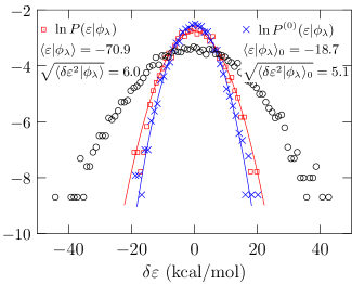
Figure S1: The coupled and uncoupled regularized binding energy distributions for the case where the separation between the terminal carbon atoms is 20.1 Å and the structure has the smallest $R_{g}$. The coupled (but not regularized) distribution is shown using open circles ($\circ$). Regularization serves to reduce the variance of this distribution. Not that despite the seemingly gaussian behavior, the high-energy tail region of the non-regularized distribution is not well characterized; it is in fact expected to obey an extreme value distribution Asthagiri et al. (2008).

Nevertheless, $\mu^{\rm ex}[P(\varepsilon|\phi_{\lambda})]=-40.5\pm 1.0$ kcal/mol is in excellent agreement with $\mu^{\rm ex}[P^{(0)}(\varepsilon|\phi_{\lambda})]=-40.4\pm 1.0$ kcal/mole. These numbers are also in excellent agreement with $-41.8$ kcal/mol obtained using the regularization approach for vdW interactions and a 2-point Gauss-Legendre quadrature for electrostatics Weber and Asthagiri (2012). The estimate $\mu^{\rm ex}(n=0|\lambda)=0.5\cdot(\langle\varepsilon|\phi_{\lambda}\rangle+\langle\varepsilon|\phi_{\lambda}\rangle_{0})=-44.8\pm 0.2$ (cf. Eq. S.4; see also Ref. 42)), which should be valid if both distributions are strictly gaussian, is also in error from the quadrature result by only about 7%.

Similar analysis was also performed for the extended state of the peptide. The final results reported are based on $\mu^{\rm ex}[P(\varepsilon|\phi_{\lambda})]$, which is particularly easy to obtain from the conditioned-peptide simulations.

S.II Enthalpic and entropic contributions to hydration

From the Euler relation for the pure solvent and the solvent with one added solute, we can show that the excess entropy of hydration is

$$Ts^{\rm ex} = E^{\rm ex}-kT^{2}\alpha_{p}+p(\langle V^{\rm ex}\rangle+kT\kappa_{T})-\mu^{\rm ex}$$ (S.5)

$$\approx E_{sw}+E_{reorg}-\mu^{\rm ex}$$

where $\kappa_{T}$ is the isothermal compressibility and $\alpha_{p}$ is the thermal expansivity of the solvent. The average excess energy of hydration, $E^{\rm ex}$, is the sum the average solute-water interaction energy $E_{sw}$ and $E_{reorg}$, the reorganization energy. The latter is given by the change in the average potential energy of the solvent in the solute-solvent system minus that in the neat solvent system. (Note that solute-solvent interactions are not counted as part of $E_{reorg}$.) Ignoring pressure-volume effects, the excess enthalpy of hydration $h^{\rm ex}=E^{\rm ex}$. The solute-solvent interaction contribution $E_{sw}$ can be further decomposed into backbone-solvent, $E_{bb}$, and sidechain-solvent, $E_{sc}$, contributions. These contributions were straightforwardly obtained using the PairInteraction module within NAMD. The coupled peptide solvent system was simulated for an additional 3 ns and frames were archived every 500 fs for interaction-energy analysis.

For calculating $E_{reorg}$ we adapted the hydration-shell-wise procedure developed earlier Asthagiri et al. (2008). We define an inner-shell around the peptide as the union of shells of radius $\lambda$ centered on the peptide heavy atoms. $\lambda\leq 5.5$ Å, $5.5<\lambda\leq 8.5$ Å, and $8.5<\lambda\leq 11.5$ Å defined the first, second, and third shells, respectively. For the reorganization calculation, the definition of the inner shell was slightly increased by 0.5 Å, but this change has no bearing on the final thermodynamic quantity $h^{\rm ex}$. Let $n_{w}$ be the number of water molecules in a shell for some chosen configuration. The potential energy of these $n_{w}$ waters is given by the interaction energy between these $n_{w}$ waters plus half the interaction energy of these $n_{w}$ waters with the rest of the fluid. We thus find the average potential energy, $\langle E_{shell}\rangle$, and the average population, $\langle n_{shell}\rangle$, for a given shell. The contribution to the average reorganization energy from the shell is then $\langle E_{shell}\rangle-\langle n_{shell}\rangle\cdot\langle\varepsilon_{w}\rangle$. Errors are propagated using standard rules.

For all cases, we find that by the third shell bulk behavior is attained; that is, $E_{reorg,3}\approx 0$ within statistical uncertainties, where $E_{reorg,3}$ is the reorganization energy contribution from the third (3^rd) shell.

S.III Distribution of hydrogen bonds versus $R_{g}$

The slight difference in the average counts versus $R_{g}$ and average counts versus $r$ (Fig. 3) occurs because the relation between $r$ and $R_{g}$ is itself subject to some statistical uncertainty. Thus sorting configurations using $r$ or $R_{g}$ as order parameters can influence the averaging of the dependent variable (here the number of hydrogen bonds). However, the physical conclusion that number of hydrogen bonds increases upon chain collapse is independent of these considerations.

References

- Kauzmann (1959) W. Kauzmann, Adv. Prot. Chem. 14, 1 (1959).
- Chandler (2005) D. Chandler, Nature 437, 640 (2005).
- Dill (1990) K. A. Dill, Biochem. 29, 7133 (1990).
- Dill and MacCallum (2012) K. A. Dill and J. L. MacCallum, Science 338, 1042 (2012).
- Teufel et al. (2011) D. P. Teufel, C. M. Johnson, J. K. Lum, and H. Neuweiler, J. Mol. Biol. 409, 250 (2011).
- Tran et al. (2008) H. T. Tran, A. Mao, and R. V. Pappu, J. Am. Chem. Soc. 130, 7380 (2008).
- Hu et al. (2010a) C. Y. Hu, G. C. Lynch, H. Kokubo, and B. M. Pettitt, Proteins: Struc. Func. Bioinform. 78, 695 (2010a).
- Cornette et al. (1987) J. L. Cornette, K. B. Cease, H. Margalit, J. L. Spouge, J. A. Berzofsky, and C. DeLisi, J. Mol. Biol. 195, 659 (1987).
- Wilce et al. (1995) M. C. J. Wilce, M.-I. Aguilar, and M. T. W. Hearn, Anal.Chem. 67, 1210 (1995).
- Möglich et al. (2006) A. Möglich, K. Joder, and T. Kiefhaber, Proc. Natl. Acad. Sc. USA 103, 12394 (2006).
- Karandur et al. (2014) D. Karandur, K.-Y. Wong, and B. M. Pettitt, J. Phys. Chem. B 118, 9565 (2014).
- Karandur et al. (2015) D. Karandur, R. C. Harris, and B. M. Pettitt, Prot. Sci. pp. 103–110 (2015).
- Weber et al. (2011) V. Weber, S. Merchant, and D. Asthagiri, J. Chem. Phys. 135, 181101 (2011).
- Weber and Asthagiri (2012) V. Weber and D. Asthagiri, J. Chem. Theory Comput. 8, 3409 (2012).
- Tomar et al. (2014) D. S. Tomar, V. Weber, B. M. Pettitt, and D. Asthagiri, J. Phys. Chem. B 118, 4080 (2014).
- Tomar et al. (2016) D. S. Tomar, W. Weber, M. B. Pettitt, and D. Asthagiri, J. Phys. Chem. B 120, 69 (2016).
- Jorgensen et al. (1983) W. Jorgensen, J. Chandrasekhar, , and M. L. Klein, J. Chem. Phys. 79, 926 (1983).
- Neria et al. (1996) E. Neria, S. Fischer, and M. Karplus, J. Chem. Phys. 105, 1902 (1996).
- Feller et al. (1995) S. E. Feller, Y. Zhang, R. W. Pastor, and B. R. Brooks, J. Chem. Phys. 103, 4613 (1995).
- Darve et al. (2008) E. Darve, D. Rodriguez-Gómez, and A. Pohorille, J. Chem. Phys. 128, 144120 (2008).
- Hénin et al. (2010) J. Hénin, G. Fiorin, C. Chipot, and M. L. Klein, J. Chem. Theory Comput. 6, 35 (2010).
- Tomar et al. (2013) D. S. Tomar, V. Weber, and D. Asthagiri, Biophys. J. 105, 1482 (2013).
- Pratt and Asthagiri (2007) L. R. Pratt and D. Asthagiri, in Free energy calculations: Theory and applications in chemistry and biology, edited by C. Chipot and A. Pohorille (Springer, Berlin, DE, 2007), vol. 86 of Springer series in Chemical Physics, chap. 9, pp. 323–351.
- Beck et al. (2006) T. L. Beck, M. E. Paulaitis, and L. R. Pratt, The potential distribution theorem and models of molecular solutions (Cambridge University Press, Cambridge, UK, 2006).
- Merchant and Asthagiri (2009) S. Merchant and D. Asthagiri, J. Chem. Phys. 130, 195102 (2009).
- Dixit et al. (2009) P. D. Dixit, S. Merchant, and D. Asthagiri, Biophys. J. 96, 2138 (2009).
- Staritzbichler et al. (2005) R. Staritzbichler, W. Gu, and V. Helms, J. Phys. Chem. B 109, 19000 (2005).
- Hu et al. (2010b) C. Y. Hu, H. Kokubo, G. Lynch, D. W. Bolen, and B. M. Pettitt, Prot. Sc. 19, 1011 (2010b).
- Kokubo et al. (2011) H. Kokubo, C. Y. Hu, and B. M. Pettitt, J. Am. Chem. Soc. 133, 1849 (2011).
- Kokubo et al. (2013) H. Kokubo, R. C. Harris, D. Asthagiri, and B. M. Pettitt, J. Phys. Chem. B 117, 16428 (2013).
- Harris and Pettitt (2014) R. C. Harris and B. M. Pettitt, Proc. Natl. Acad. Sc. USA 111, 14681 (2014).
- Pratt and Pohorille (1992) L. R. Pratt and A. Pohorille, Proc. Natl. Acad. Sc. USA 89, 2995 (1992).
- Pratt (2002) L. R. Pratt, Ann. Rev. Phys. Chem. 53, 409 (2002).
- Rose et al. (2006) G. D. Rose, P. J. Fleming, J. R. Banavar, and A. Maritan, Proc. Natl. Acad. Sc. USA 103, 16623 (2006).
- Bolen and Rose (2008) D. W. Bolen and G. D. Rose, Annu. Rev. Biochem. 77, 339 (2008).
- Auton et al. (2011) M. Auton, J. Rösgen, M. Sinev, L. M. Holthauzen, and D. W. Bolen, Biophys. Chem. 159, 90 (2011).
- Kale et al. (1999) L. Kale, R. Skeel, M. Bhandarkar, R. Brunner, A. Gursoy, N. Krawetz, J. Phillips, A. Shinozaki, K. Varadarajan, and K. Schulten, J. Comput. Phys. 151, 283 (1999).
- Hummer and Szabo (1996) G. Hummer and A. Szabo, J. Chem. Phys. 105, 2004 (1996).
- Friedberg and Cameron (1970) R. Friedberg and J. E. Cameron, J. Chem. Phys. 52, 6049 (1970).
- Allen and Tildesley (1987) M. P. Allen and D. J. Tildesley, Computer simulation of liquids (Oxford University Press, 1987), chap. 6. How to analyze the results, pp. 192–195.
- Asthagiri et al. (2008) D. Asthagiri, S. Merchant, and L. R. Pratt, J. Chem. Phys. 128, 244512 (2008).
- Rogers and Beck (2008) D. M. Rogers and T. L. Beck, J. Chem. Phys. 129, 134505 (2008).