A Monte-Carlo Method for Estimating Stellar Photometric Metallicity Distributions

Abstract

Based on the Sloan Digital Sky Survey (SDSS), we develop a new monte-carlo based method to estimate the photometric metallicity distribution function (MDF) for stars in the Milky Way. Compared with other photometric calibration methods, this method enables a more reliable determination of the MDF, in particular at the metal-poor and metal-rich ends. We present a comparison of our new method with a previous polynomial-based approach, and demonstrate its superiority. As an example, we apply this method to main-sequence stars with $0.2<g-r<0.6$, $6$ kpc$<R<9$ kpc, and in different intervals in height above the plane, $|Z|$. The MDFs for the selected stars within two relatively local intervals ($0.8$ kpc$<|Z|<1.2$ kpc, $1.5$ kpc$<|Z|<2.5$ kpc) can be well-fit by two Gaussians, with peaks at [Fe/H] $\approx-0.6$ and $-1.2$ respectively, one associated with the disk system, the other with the halo. The MDFs for the selected stars within two more distant intervals ($3$ kpc$<|Z|<5$ kpc, $6$ kpc$<|Z|<9$ kpc) can be decomposed into three Gaussians, with peaks at [Fe/H] $\approx-0.6$, $-1.4$ and $-1.9$ respectively, where the two lower peaks may provide evidence for a two-component model of the halo: the inner halo and the outer halo. The number ratio between the disk component and halo component(s) decreases with vertical distance from the Galactic plane, consistent with the previous literature.

1. Introduction

The metallicity distribution function (MDF) for stars in the Milky Way is of great importance to reveal the chemical structure of Galactic halo and disk systems, and provides essential clues to the assembly and enrichment history of the Galaxy (Carollo et al., 2007, 2010; Peng et al., 2012, 2013; An et al., 2013, 2015). Many multi-fiber spectroscopic surveys, including the Sloan Digital Sky Survey (SDSS; York et al., 2000), the Radial Velocity Experiment (RAVE; Steinmetz et al., 2006), and the Large Sky Area Multi-Object Fiber Spectroscopic Telescope (LAMOST; Deng et al., 2012; Liu et al., 2014; Zhao et al., 2012), have obtained metallicity estimates and other stellar parameters for millions of stars from low- and medium-resolution spectra. However, compared with photometric data, the number of spectra within the limiting magnitudes of the surveys is still too small to provide a detailed chemical map of the Galaxy, even in the relatively local region. The use of photometric data, which is available for far more stars than the spectroscopic data, breaks through this limitation.

Considering that the exhaustion of metals in a stellar atmosphere has a detectable effect on the emergent flux (Schwarzschild et al., 1955), in particular in the blue region where the density of metal absorption is highest, the combination of spectroscopic data and photometric data can be used to derive estimates of [Fe/H] (Allende Prieto et al., 2006, 2008; Lee et al., 2008a, b). For example, Siegel et al. (2009) derived approximate stellar metallicities through measurement of the ultraviolet excess, based on $UBV$ data in SA 141. Ivezić et al. (2008) employed SDSS data to derive a metallicity estimator from $u-g$ and $g-r$ colors, and successfully mapped the metallicity distribution of millions of F/G main-sequence stars within a distance of $\sim 8$ kpc from the Sun. Peng et al. (2012) also used BATC survey data to estimate the stellar photometric metallicity distribution. Gu et al. (2015) obtained a metallicity estimator using SCUSS (Zou et al., 2015a, b) data, which can be applied up to fainter magnitudes due to the use of more accurate SCUSS $u$-band measurements, and used it to explore the metallicity of the Sagittarius stream in the South Galactic cap. Using a minimum $\chi^{2}$ technique, Yuan et al. (2015) estimated photometric metallicities simultaneously using the dereddened colors $u-g$, $g-r$, $r-i$, and $i-z$ from the SDSS and metallicity-dependent stellar loci. An et al. (2013) calibrated stellar isochrones to derive metallicities of individual stars with SDSS $ugriz$ photometry. An et al. (2015) applied this method to recently improved co-adds of $ugriz$ photometry for Stripe 82 from SDSS, including a factor of two more stars than their previous effort. The new analysis revealed a MDF for halo stars between 5 and 10 kpc from the Sun with peak metallicities at [Fe/H] $\sim-1.4$ and [Fe/H] $\sim-1.9$, which the authors associated with the inner-halo and outer-halo populations of the Milky Way, respectively.

The photometric metallicity calibrations developed by previous works are characterized by their assignment of a star-by-star metallicity estimate based on its color indexes. This inevitably introduces error, because a single star's metallicity is actually uncertain even when its color indexes are fixed, varying around the metallicity estimate to form a distribution. In addition, the calibration methods used by Ivezić et al. (2008) and Gu et al. (2015) yield poor results for very metal-rich or very metal-poor stars. However, in order to investigate the chemical structure of the Galactic stellar populations, we only require knowledge of the MDF for a large statistical sample of stars. Here we develop a monte-carlo method to estimate the photometric metallicity distribution of large number of stars with available SDSS photometry.

This paper is organized as follows. In Section 2, we provide a brief overview of the SDSS and its photometric data. Details of our monte-carlo based photometric metallicity calibration are presented in Section 3. Section 4 presents a comparison between this method and the more traditional polynomial-fitting method. As an example, in Section 5 we apply this method to derive the MDF for Galactic stars and consider its variation with height above the plane. A brief summary is given in Section 6.

2. SDSS photometric data

The SDSS is a large international collaboration project, and it has obtained deep, multi-color images covering more than one-quarter of the celestial sphere in the North Galactic cap, as well as a small ($\sim 300$ deg²), but much deeper survey, in the South Galactic hemisphere (York et al., 2000). The SDSS used a dedicated 2.5-meter telescope at Apache Point Observatory, New Mexico (Gunn et al., 2006). The flux densities are measured in five bands ($u$, $g$, $r$, $i$, $z$) with effective wavelengths of 3551, 4686, 6165, 7481 and 8931 Å, respectively. The $95\%$ completeness limits of the images are 22.0, 22.2, 22.2, 21.3, and 20.5 for $u$, $g$, $r$, $i$, and $z$, respectively (Abazajian et al., 2004). The relative photometric calibration accuracy for $u$, $g$, $r$, $i$, and $z$ are 2%, 1%, 1%, 1% and 1%, respectively (Padmanabhan et al., 2008). Figure 1 shows the error of $u$-, $g$-, and $r$-band magnitude as a function of $g$-band magnitudes. Other technical details about SDSS can be found on the SDSS website http://www.sdss3.org/, which also provides an interface for the public data access.

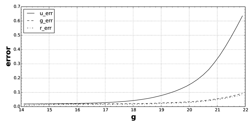
Figure 1.— The average magnitude error of numerous stars as a function of $g$ magnitude. Main-sequence stars with $0.2<g-r<0.8$ and $0.6<u-g<2.2$ are selected. The $u$ magnitude error is much larger than that of $g$ and $r$, especially at the faint end.

The Sloan Extension for Galactic Understanding and Exploration (SEGUE-1) obtained spectra of nearly 230,000 unique stars over a range of spectral types to investigate Galactic structure. Building on this success, SEGUE-2 spectroscopically observed around 119,000 unique stars, focusing on the stellar halo of the Galaxy, including stars with distance from 10 to 60 kpc from the Sun. We employ the complete set of derived stellar parameters for SEGUE-1 and SEGUE-2 from the newest version of SEGUE Stellar Parameter Pipeline (SSPP; Beers et al., 2006; Lee et al., 2008a, b; Allende Prieto et al., 2008; Smolinski et al., 2011; Lee et al., 2011), including effective temperature, surface gravity, and metallicity (parameterized as [Fe/H]). A thorough overview of SEGUE effort can be found in Yanny et al. (2009).

We use the adopted stellar atmospheric parameters from the SSPP listed in the sppParams table. After excluding the repeated stars surveyed on different plates, we obtain a sample of 366,676 stars with SDSS $u,g,r,i,and~{}z$ magnitudes, as well as stellar parameters. Most stars in the sample have metallicities in the range $-2.5\leq$[Fe/H]$\leq 0.0$. In this study, in order to generate the [Fe/H] probability distribution from the colors, we select main-sequence stars, adopting the following selection criteria:

• $14<g<19.5$;

• $0.2<g-r<0.8$;

• $0.6<u-g<2.2$;

• Main-sequence stars are selected by rejecting those objects at distances larger than $0.15$ mag from the stellar locus described by following equation (Jurić et al., 2008):

  $$g-r= 1.39\{1-exp[-4.9(r-i)^{3}-2.45(r-i)^{2}$$

  $$-1.68(r-i)-0.05]\}$$

• We further refine the selection of main-sequence stars by rejecting those objects at distances larger than $0.3$ mag from the stellar locus described by the following equation (Jia et al., 2014):

  $$u-g=exp[-(g-r)^{2}+2.8(g-r)-1]$$

As an illustration, Figure 2 shows the two-color diagrams for $r-i$ versus $g-r$ and $u-g$ versus $g-r$. Our final sample includes 268,029 sample stars. Throughout this paper it is understood that magnitude and color have been corrected for extinction and reddening following Schlegel et al. (1998).

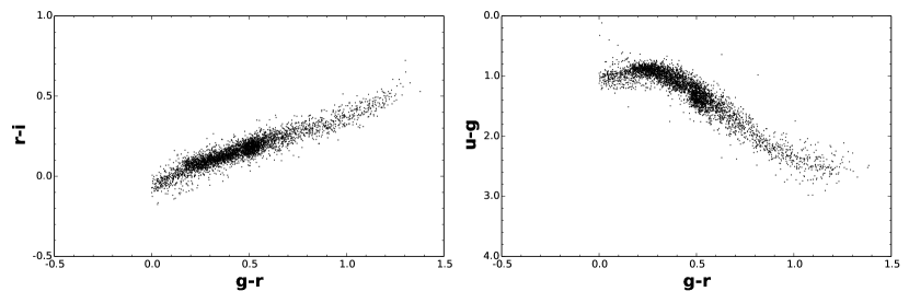
Figure 2.— Main-sequence stars selection from two-color diagrams. In the left panel ($r-i$ vs. $g-r$), we reject those objects at distances larger than $0.15$ mag from the stellar locus. In the right panel ($u-g$ vs. $g-r$), we further refine the selection of main-sequence stars by rejecting those objects at distances larger than $0.3$ mag from the stellar locus.

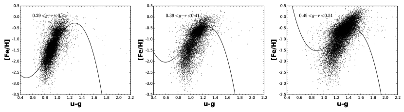
Figure 3.— The scatter distribution of spectroscopic [Fe/H] versus $u-g$ color for main-sequence stars with $g-r$ color specified in a small color interval, as shown in the legends of each panel. The three solid lines are generated from the photometric metallicity estimator derived by Ivezić et al. (2008), with $g-r=0.3$ for the left panel, $g-r=0.4$ for the middle panel, and $g-r=0.5$ for the right panel.

3. Method

Figure 3 shows the spectrum-determined [Fe/H] distribution of stars versus $u-g$ color. These stars are selected within small color ranges around $g-r=0.3$, $g-r=0.4$ and $g-r=0.5$. The solid lines represent the photometric metallicity estimator derived by Ivezić et al. (2008) with $g-r$ color specified by 0.3, 0.4, and 0.5 respectively. From inspection of this Figure, these lines can only roughly describe the relation between [Fe/H] and $u-g$ color. Those stars with specified $u-g$ and $g-r$ colors exhibit a metallicity distribution which may result from several other factors. We build the metallicity probability distribution from the scattered points in each specified color bin, and then use a monte-carlo method to infer the MDF for large numbers of stars. That is to say, what we obtain from our photometric calibration is not a one-to-one function, but a probability-governed one-to-many function.

The monte-carlo method relies on repeated random sampling to obtain numerical results. As mentioned in the selection criteria, the two colors we employ are confined to $0.2<g-r<0.8$ and $0.6<u-g<2.2$. We divided the $u-g$ vs. $g-r$ panel into $0.05\times 0.05$ mag² bins, and designate each square unit by an index computed in the following manner:

$$index=int((u-g-0.6)/0.05)*12+int((g-r-0.2)/0.05)\text{,}$$

where the symbol $int$ stands for the integer portion. We obtain 384 square units. For a given sample of stars, we also divided the value of [Fe/H] from -3.5 to 0.5 into 80 bins equally, with a bin width of 0.05 dex. In this manner, we obtained an array of index $\times$ [Fe/H]. Each array element records the number of stars whose colors and [Fe/H] match their corresponding positions, based on the above-selected sample of 268,029 stars. The resulting array, with its array elements holding the pertinent information, is called the ``seed'' array. Each element of the seed array is denoted by $value[index][i]$, where $i$ ranges from 0 to 79. The maximum of $value[index][i]$ for $i$ in the range $[0,79]$ can easily be found, and is denoted by $max[index]$. From this seed array, we can evaluate the MDF for the photometrically-surveyed stars.

For a certain index ($u-g$ and $g-r$ interval), we use the monte-carlo method to generate a random number sequence whose probability distribution is determined by the [Fe/H] distribution recorded in the seed array. Suppose $X$ and $Y$ are two stochastic variables which can be assigned a value by a random number generating function $rand_{X}()$ and $rand_{Y}()$, respectively. The function $rand_{X}()$ is modulated to generate a uniform-probability distributed random integer number from 0 to 79, and $rand_{Y}()$ from 0 to $max[index]$. In each trial, we obtain a random number pair ($X=rand_{X}()$, $Y=rand_{Y}()$). When $Y\leq value[index][X]$, we record $X$ as a useful value, otherwise we discard it. By numerous trials, we obtain a sequence of random numbers {$X_{1},X_{2},X_{3},\cdots$} that follow the same probability distribution as those recorded in the seed array. Then we can transform the obtained random number sequence into metallicities, [Fe/H], by [Fe/H]=$0.05*index-3.5+0.025$. Here, because $value[index][i]$ can be equal to zero for some $i$ values, we can discard them and record the non-zero elements and their positions in a new array. Through this trick, we greatly improve the sampling efficiency.

For a large number of photometrically-surveyed stars, we first count the number of stars that corresponds to each array element, and then, following the above procedure, obtain metallicities of the counted number for all array elements. The metallicities naturally form a distribution which we discuss below.

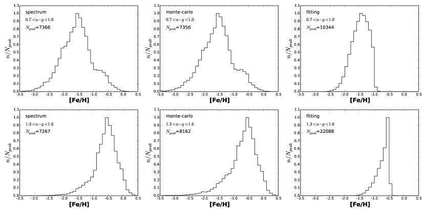
Figure 4.— The metallicity distribution of spectroscopically-surveyed main-sequence stars in the color range $0.2<g-r<0.6$. The top three panels show the metallicity distribution of stars with $0.7<u-g<1.0$, and the bottom three with $1.3<u-g<1.6$. The left panels present the spectrum-based metallicity distribution. The middle panels show the photometric metallicity distribution determined by the monte-carlo method, and the right panels show the photometric metallicity distribution from Ivezić et al. (2008)'s model. The peak values in all the histograms are normalized to one, with the actual values shown in the legends of each panel.

4. Comparison

To test the feasibility, and to show the superiority of the method described above, we make a comparison between this monte-carlo based method and the third-order polynomial-fitting method presented in Ivezić et al. (2008), shown below:

$$\rm[Fe/H]= -4.37-8.56x+15.5y+23.5x^{2}$$

$$-39.0xy+20.5y^{2}-10.1x^{3}$$

$$+12.1x^{2}y+7.33xy^{2}-21.4y^{3}\text{,}$$

where $x=u-g$ for $(g-r)<0.4$ and $x=(u-g)-2(g-r)+0.8$ for $(g-r)>0.4$, $y=g-r$.

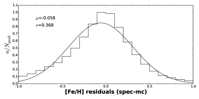
Figure 5.— The distribution of the [Fe/H] residuals between the spectrum-based metallicity and that derived by the monte-carlo method for individual stars. Main-sequence stars are selected with $0.2<g-r<0.6$. This distribution is fitted by a Gaussian, with its mean zero-point offset and dispersion values labeled.

We select main-sequence stars covering the color range $0.2<g-r<0.6$ from the spectroscopically-surveyed stars and evaluate their photometric metallicity distribution. Figure 4 shows the derived MDFs from the three different methods. The top three panels show the MDFs for stars with $0.7<u-g<1.0$, and the bottom three panels with $1.3<u-g<1.6$. The left panels present the spectrum-based MDF which can be regarded as ``ground truth''. The middle panels show the photometric MDF determined by our monte-carlo method, and the right panels show the photometric MDF from Ivezić et al. (2008)'s model. The peak values in all the histograms are normalized to one, with the actual peak values labeled. As shown in Figure 4, the photometric MDFs based on our monte-carlo method much more closely resemble the spectroscopic MDFs than those obtained from the Ivezić et al. (2008) approach. Not only are the peak values of the photometric MDFs determined by our monte-carlo method approximately equal to those of the spectrum-based MDF, but the wings of the two distributions have almost the same profile. By contrast, there exists some clear discrepancies between the photometric MDFs from Ivezić et al. (2008)'s model and the spectrum-based MDFs, particularly at the very metal-rich and very metal-poor ends. We thus believe that polynomial-based fitting methods are clearly inferior, and should no longer be generally used. For application to a large number of stars, there is great advantage in using the monte-carlo method for the derivation of photometric MDFs. Note that if the number of stars used to evaluate the photometric MDFs is small, we can easily increase the number of desired random numbers $X$ using a multiplicative factor in the monte-carlo method.

Figure 5 shows the distribution of metallicity residuals between the spectrum-based metallicity and that determined by the monte-carlo method for individual stars. We determine the metallicity of a single star from the peak value of the metallicity distribution in each specific color bin. The stars are selected covering the color range $0.2<g-r<0.6$. The distribution is roughly a Gaussian profile, with mean zero-point offset of $-0.058$ dex and dispersion of $0.368$ dex.

In the conventional photometric metallicity calibration by polynomial fitting, the error mainly arises from two sources. One is from the fitting method itself (illustrated in Figure 3), and the other is from the errors in the color indexes. In SDSS, the photometric error of the $u$-band magnitude is relatively large (shown in Figure 1), limiting the application range of the photometric metallicity estimator. In the monte-carlo calibration method, we suppose that the spectrum-based metallicity distribution in a given $u-g$, $g-r$ color bin is fairly reliable, and thus, by reproducing its distribution we effectively eliminate the errors arising from the fitting method. The error introduced by fluctuations in the monte-carlo method can be eliminated by increasing the number of desired random numbers. In addition, the third-order polynomial model is determined by only 10 coefficients, while the model (seed array) construction involves many more variables. This, to some extent, guarantees the accuracy of photometric metallicity distribution determined by the monte-carlo method. The deviation of the photometric MDF determined by the monte-carlo method mainly arises from the errors in the color indexes, especially when estimating the MDFs for faint stars. As shown in Figure 4, the calibration based on the monte-carlo method can be used to derive photometric MDFs with sufficient accuracy for most purposes.

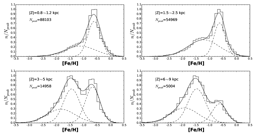
Figure 6.— Photometric MDFs derived by the monte-carlo method. Main-sequence stars with $0.2<g-r<0.6$, 6 kpc$<R<$9 kpc, and distance from the Galactic plane in the range $0.8\sim 1.2$ kpc (top left panel), $1.5\sim 2.5$ kpc (top right panel), $3\sim 5$ kpc (bottom left panel), $6\sim 9$ kpc (bottom right panel) are selected as samples. The peak values in these four histograms are all normalized to one, with actural values labeled. The top two MDFs can be well-fit by two Gaussians with peaks at $-0.6$ (disk contribution) and $-1.2$ (halo contribution) respectively. The bottom two MDFs are better-fit by three Gaussians, with peaks respectively at $-0.6$, $-1.4$ and $-1.9$.

5. Application

As an example, we use the method introduced in this study to derive the photometric MDF for stars as a function of distance from the Galactic plane. The main-sequence stars with $0.2<g-r<0.6$, $6$ kpc $<R<9$ kpc, and in different $|Z|$ intervals are selected ($R$, $Z$ represent cylindrical Galactocentric coordinates, with the Sun's coordinate $(R,~{}Z,~{}\phi)=$(8 kpc, 0, 0)). As shown in Figure 6, the photometric MDFs in the top two panels can be well-fit by two Gaussians, with peaks at about $-0.6$ and $-1.2$ respectively, one associated with the disk system, and the other with the halo (and metal-weak disk). The MDFs in the two bottom panels are found to be better-fit by three Gaussians, with peaks at about $-0.6$, $-1.4$ and $-1.9$, respectively. The two lower peaks may be associated with inner-halo and outer-halo populations, respectively (Carollo et al., 2007, 2010; An et al., 2013, 2015). These four histograms clearly show that the number ratio between disk stars and halo stars decreases with vertical distance from the Galactic plane. In the metal-rich and metal-poor ends, the number of stars decrease gradually. The number ratios as a function of $|Z|$ between the disk and halo above the Galactic plane could be recalculated from the photometric metallicity distribution, and the result can be compared with that from the method of star counting. This will be presented in our future papers.

6. Summary

This paper presents a new method to estimate the photometric MDF for main-sequence stars. The method is tested using a spectroscopic sample of stars from the SDSS. Compared with the method from Ivezić et al. (2008), the current method is more accurate, particularly for very metal-rich and very metal-poor stars. This method is sufficiently accurate to be used to investigate the distribution and chemical structure of the Galactic stellar populations. At the same time, as an example, we also apply the method to the main-sequence stars with $0.2<g-r<0.6$, $6$ kpc $<R<9$ kpc, and different $|Z|$ intervals. The metallicity distribution of sample stars near the Galactic plane can be well-fit by two Gaussians, with peaks at about $-0.6$ and $-1.2$, respectively, one associated with the disk system and the other with the halo/metal-weak thick disk. However, the metallicity distribution of the sample stars far from the Galactic plane can be well-fit by three Gaussians, with peaks at $-0.6$, $-1.4$ and $-1.9$, which supports the existence of two components in the halo: the inner-halo and the outer-halo. The number ratio between disk stars and halo stars varies with vertical distance from the Galactic plane. In the metal-rich and metal-poor ends, the number of stars decreases gradually. With the advantage of the method introduced in this paper, we can better study the photometric MDF for different stellar populations in the Galaxy and provide detailed constraints on the Galactic chemical evolution, which we will consider in future papers.

References

- An et al. (2013) An, D., Beers, T. C., Johnson, J. A., et al. 2013, ApJ, 763, 65
- An et al. (2015) An, D., Beers, T. C., Santucci, R. M., et al. 2015, ApJ, 813, L28
- Abazajian et al. (2004) Abazajian, K., Adelman-McCarthy,J.K., et al. 2004, AJ, 128, 502
- Allende Prieto et al. (2006) Allende Prieto, C., Beers, T. C., Wilhelm, R., et al. 2006, ApJ, 636, 804
- Allende Prieto et al. (2008) Allende Prieto, C., Sivarani, T., Beers, T. C., et al. 2008, AJ, 136, 2070
- Beers et al. (2006) Beers, T., C., Lee, Y., Sivarani, T., et al. 2006, Mem. Soc. Astron. Italiana, 77, 1171
- Carollo et al. (2007) Carollo, D., Beers, T. C., Lee, Y. S., et al. 2007, Nature, 450, 1020
- Carollo et al. (2010) Carollo, D., Beers, T. C., Chiba. M., et al. 2010, ApJ, 712, 692
- Deng et al. (2012) Deng, L.C., Newberg, H., Liu, C., et al. 2012, RAA, 12, 735
- Gu et al. (2015) Gu, J. Y., Du, C. H., Jia, Y. P., et al. 2015, MNRAS, 452, 3092
- Gunn et al. (2006) Gunn, J. E., Siegmund, W. A., Mannery, E. J., et al. 2006, AJ, 131, 2332
- Ivezić et al. (2008) Ivezić, Ž., Sesar, B., Jurić, M., et al. 2008, ApJ, 684, 287
- Jurić et al. (2008) Jurić, M., Ivezić, Ž., Brooks, A., et al. 2008, ApJ, 673, 864
- Jia et al. (2014) Jia, Y. P., Du, C. H., Wu, Z. Y., et al. 2014, MNRAS, 441, 503
- Liu et al. (2014) Liu, X.W., Yuan, H.B., Huo, Z.Y., et al. 2014, in Proc. IAU Symp. 29, Setting the Scene for Gaia and LAMOST, ed. S. Feltzing, G. Zhao, N. Walton, & P. Whitelock (Cambridge: Cambridge University Press), 310
- Lee et al. (2008a) Lee, Y. S., Beers, T. C., Sivarani, T., et al. 2008, AJ, 136, 2050
- Lee et al. (2008b) Lee, Y. S., Beers, T. C., Sivarani, T., et al. 2008, AJ, 136, 2022
- Lee et al. (2011) Lee, Y. S., Beers, T. C., Allende Prieto, C., et al. 2011, AJ, 141, 90
- Padmanabhan et al. (2008) Padmanabhan, N., Schlegel, D. J., Finkbeiner, D. P., et al. 2008, ApJ, 674, 1217
- Peng et al. (2013) Peng, X. Y., Du, C. H., Wu, Z. Y., Ma, J., & Zhou, X. 2013, MNRAS, 434, 3165
- Peng et al. (2012) Peng, X.Y., Du, C.H., Wu, Z.Y., 2012, MNRAS, 422, 2756
- Schlegel et al. (1998) Schlegel, D. J., Finkbeiner, D. P., & Davis, M. 1998, ApJ, 500, 525
- Schwarzschild et al. (1955) Schwarzschild, M., Searle, L., & Howard, R. 1955, ApJ, 122, 353
- Siegel et al. (2009) Siegel, M. H., Karatas, Y., Reid, I. N., 2009, MNRAS, 395, 1569
- Steinmetz et al. (2006) Steinmetz, M., Zwitter, T., Siebert, A., et al. 2006, AJ, 132, 1645
- Smolinski et al. (2011) Smolinski, J. P., Lee, Y. S., Beers, T. C., et al. 2011, AJ, 141, 89
- Yanny et al. (2009) Yanny, B., Newberg, H. J., Johnson, J. A., et al. 2009, ApJ, 700, 1282
- York et al. (2000) York, D. G., Adelman, J., Anderson, J. E., Jr., et al. 2000, AJ, 120, 1579
- Yuan et al. (2015) Yuan, H. B., Liu, X. W., Xiang, M. S., et al. 2015, ApJ, 803, 13
- Zou et al. (2015a) Zou, H., Zhou, X., Jiang, Z. J., et al., 2015, AJ, 150, 104
- Zou et al. (2015b) Zou, H., Zhou, X., Jiang, Z. J., et al., 2016, AJ, 151, 37
- Zhao et al. (2012) Zhao, G., Zhao, Y. H., Chu, Y. Q., et al. 2012, RAA, 12, 723