Entropy production by active particles: Coupling of odd and even functions of velocity

Abstract

Non-equilibrium stochastic dynamics of several active Brownian systems are modeled in terms of non-linear velocity dependent force. In general, this force may consist of both even and odd functions of velocity. We derive the expression for total entropy production in such systems using the Fokker-Planck equation. The result is consistent with the expression for stochastic entropy production in the reservoir, that we obtain from probabilities of time-forward and time-reversed trajectories, leading to fluctuation theorems. Numerical simulation is used to find probability distribution of entropy production, which shows good agreement with the detailed fluctuation theorem.

I Introduction

Active particles are self propelled entities that perform locomotion utilizing internal energy, even in the absence of an external driving force. The internal energy source may be replenished by food, e.g., in animal to bacteria, or local chemical fuel in the form of ATP in molecular motors. Studies of active particles have been motivated by dynamic cluster formation in birds, fish, or animal Vicsek2012 ; Vicsek1995 , active Brownian motion of self propelled colloids or nano rotors Howse2007 ; Zheng2013 ; Nourhani2013 , and even by the motion of vibrated granular systems Feitosa2004 ; Joubaud2012 ; Kumar2011 . The self propelled motion of several active Brownian particle (ABP) systems may be described in terms of a non-linear velocity dependent force Romanczuk2012 ; Badoual2002 ; Julicher1995 .

A simple example of non-linear velocity dependent force is the motion of a projectile through a compressible fluid. A particle of velocity $v$ displaces a volume of fluid proportional to $v$, thus imparting a change in momentum proportional to $v^{2}$ in the medium per unit time. The particle in turn encounters an equal and opposite force, which is an even function of $v$ but directed opposite to the direction of motion. In an active system, on the other hand, non-linear velocity dependent force may support the motion at small velocities. Two such models are the Rayleigh-Helmholtz model Romanczuk2012 , and the energy depot model Schweitzer1998 ; Zhang2008 .

Systems with small degrees of freedom (dof), and driven arbitrarily out of equilibrium are describable within the framework of stochastic thermodynamics Sekimoto1998 ; Bustamante2005 ; Seifert2012 . This uses stochastic counterparts of thermodynamic observables like work, entropy etc. The detailed fluctuation theorem imposes strict symmetry to the probability distribution of entropy production in passive Brownian systems driven out of equilibrium, e.g., small assembly of nano-particles, colloids, granular matter, and polymers Jarzynski2011 ; Jarzynski1997 ; Crooks1999 ; Wang2002 ; Liphardt2002 ; Feitosa2004 ; Narayan2004 ; Kurchan2007 . Although stochastic entropy production (EP) can be negative, probability of such events is exponentially suppressed with respect to positive entropy producing trajectories Evans1993 ; Gallavotti1995 ; Lebowitz1999 ; Seifert2005 ; Seifert2008 . Stochastic thermodynamics of dry friction has been considered recently Gnoli2013 ; Sarracino2013 ; Cerino2015 . In the context of coarse grained theories, it is known that simplification of a model by integrating out faster dofs leads to loss of information and EP Puglisi2010 ; Crisanti2012 ; Mehl2012a ; Jia2016 .

Several experiments on colloids and granular matter were used to verify fluctuation theorems Wang2002 ; Blickle2006 ; Speck2007 ; Joubaud2012 . Using Jarzynski equality, the free energy landscape of RNA was obtained from distribution of non-equilibrium work done Liphardt2002 ; Collin2005 . Fluctuation theorems have been derived for models of molecular motors as well Seifert2011 ; Lacoste2011 ; Lacoste2009 . Autonomous torque generation by rotary motor was estimated applying detailed fluctuation theorem on stochastic trajectories Hayashi2010 ; Hayashi2012 . Stochastic thermodynamic description of the Rayleigh-Helmholtz and energy depot model were obtained recently Ganguly2013 ; Chaudhuri2014 .

In this paper, we study stochastic thermodynamics for ABPs in the presence of general velocity dependent forces containing both odd and even functions of velocity. Unlike the Rayleigh-Helmholtz model, the presence of an even function of velocity, and its coupling with the odd function leads to EP in velocity space even in the absence of external force or potential. Using the Fokker-Planck equation, we derive the expression for total EP in the reservoir. The result is consistent with the expression for stochastic EP that we find independently from the probability distributions of time forward and time reversed trajectories. This gives us several excess entropy terms, in addition to Clausius like dependence of stochastic EP on stochastic heat flux. We further discuss the amount of loss of EP inherent to a coarse grained model of ABP, like the Rayleigh-Helmholtz model, with self propulsion in absence of a mechanism behind it, by explicitly considering an energy depot like mechanism producing activity. The path probability calculations of the ABP model lead to detailed and integral fluctuation theorems (FT) for EP. Finally, we use numerical simulations to find the probability distribution of EP that shows good agreement with the detailed FT.

II Non-linear velocity dependent force

The dynamics of this ABP under non-linear velocity dependent forces $F(v)=\zeta(v)+\xi(v)$ such that $\zeta(-v)=-\zeta(v)$ and $\xi(-v)=\xi(v)$ is described by the Langevin equations of motion

$$\dot{x} = v$$

$$\dot{v} = \eta(t)+g(v)+\xi(v)-\partial_{x}U(x)+f(t).$$ (1)

where $g(v)=-\gamma v+\zeta(v)$ denotes an odd function of velocity with $-\gamma v$ the viscous dissipation due to surrounding environment, $\eta(t)$ is the Gaussian white noise obeying $\langle\eta(t)\rangle=0$, $\langle\eta(t)\eta(t^{\prime})\rangle=2D_{0}\delta(t-t^{\prime})$ with $D_{0}=\gamma k_{B}T$, with $k_{B}$ the Boltzmann constant, and $T$ is the temperature of surrounding heat bath. $U(x)$ is an external potential, and $f(t)$ a time-dependent control force. We use particle mass $m=1$ throughout this paper.

The Fokker-Planck equation corresponding to Eq.(1) is given by

$$\partial_{t}P(x,v,t) = -\partial_{x}(vP)-\partial_{v}\left[\left(g(v)+\xi(v)+\bar{\cal F}\right)P\right]$$ (3)

$$+D_{0}\partial_{v}^{2}P\equiv-\nabla.{\bf j}$$

where $\nabla=(\partial_{x},\partial_{v})$, $g(v)$ and $\xi(v)$ are odd and even functions of velocity, respectively, and $\bar{\cal F}=f(t)-\partial_{x}U$. Under time reversal, position $x$ is an even variable, and velocity $v$ is an odd variable. The probability current ${\bf j}={\bf j}_{r}+{\bf j}_{d}$ with ${\bf j}_{r}=[vP,(\bar{\cal F}+\xi(v))\,P]$ the time-reversal symmetric part, and ${\bf j}_{d}=(0,g(v)P-D_{0}\partial_{v}P)$ the dissipative part. Note that when ${\bf j}_{d}=(0,0)$, FP equation remains invariant under time reversal. Whereas, if ${\bf j}_{r}=(0,0)$, the right hand side of FP equation picks up an overall negative sign. The presence of dissipative current ${\bf j}_{d}$ denotes breaking of time-reversal symmetry and entropy production (EP).

The model presented here should be interpreted as a coarse grained model of self propulsion, incorporating an internal energy source for each particle. Assuming a time scale separation of the internal degrees of freedom (dof) with respect to the relatively slow mechanical motion of the particles, one can integrate out these fast internal dof. An assumption of steady state for these internal dof allows one to effectively incorporate them via a velocity dependent force in mechanical motion Schweitzer1998 . Note that this force renders an inherently non-equilibrium nature to the ABPs. Even in a special case of detailed balance in the mechanical dof for $\xi(v)=0$, this dissipative probability current from internal energy source to mechanical motion leaves the particle out of equilibrium, a fact reflected in their non-Gaussian steady state velocity distribution Chaudhuri2014 .

III Entropy production

III.1 From the Fokker-Planck equation

We first calculate EP using the FP equation. The definition of non-equilibrium Gibbs entropy $S(t)=-k_{B}\int dx\,dvP(x,v,t)\ln P(x,v,t)$, along with the FP equation, may be used to obtain the rate of EP,

$$\frac{dS}{dt} = -k_{B}\int dx\,dv\,\ln P\,\frac{\partial P}{\partial t}$$ (4)

$$= k_{B}\int dx\,dv\,\ln P\,[\nabla\cdot({\bf j}_{r}+{\bf j}_{d})].$$ (5)

In obtaining the first step, we used the normalization condition of $P$ that leads to $\int dx\,dv\,\partial_{t}P=0$. Integration by parts twice,

$$\int dx\,dv\,\ln P\,\nabla\cdot{\bf j}_{r}=\int dx\,dv\,P\,\nabla\cdot({\bf j}_{r}/P)=\langle\partial_{v}\xi(v)\rangle$$

using ${\bf j}_{r}/P=[v,(\bar{\cal F}+\xi(v))]$ in the last step. The integral involving dissipative current, leads to

$$\int dx\,dv\,\ln P\,\nabla\cdot{\bf j}_{d}=-\int dx\,dv\,{j}_{d}\,\frac{g(v)-{j}_{d}/P}{D_{0}}.$$

In deriving the above relation, we used the expression of the velocity component of dissipative current ${j}_{d}=g(v)P-D_{0}\partial_{v}P$ to write $\partial_{v}\ln P$ in terms of ${j}_{d}$. Thus,

$$\frac{1}{k_{B}}\frac{dS}{dt} = \langle\partial_{v}\xi(v)\rangle+\int dx\,dv\frac{{j}_{d}^{2}}{P\,D_{0}}-\frac{1}{D_{0}}\int dx\,dv\,{j}_{d}g(v).$$

This leads to the total EP

$$\dot{S}_{t}=\dot{S}+\dot{S}_{r}=k_{B}\int dx\,dv\frac{{j}_{d}^{2}}{P\,D_{0}}\geq 0$$ (6)

in agreement with the second law of thermodynamics. This is characterized by the dissipative non-equilibrium processes in the system in terms of ${j}_{d}$. The entropy flux to reservoir is the same as the EP in reservoir

$$\frac{1}{k_{B}}\dot{S}_{r}=-\langle\partial_{v}\xi(v)\rangle+\frac{1}{D_{0}}\int dx\,dv\,{j}_{d}g(v).$$ (7)

The definition $S(t)=-k_{B}\int dx\,dvP\ln P$ leads to the definition of stochastic entropy in the system $s(t)=-k_{B}\ln P(x,v,t)$ such that $S(t)=\langle s(t)\rangle$ Seifert2005 . Similarly the stochastic EP in reservoir $\dot{s}_{r}$ is expected to obey $\dot{S}_{r}=\langle\dot{s}_{r}\rangle$. The thermodynamic average of stochastic quantities involve a two step averaging, (i) over trajectories, (ii) over phase space with probability $P(x,v,t)$ Seifert2005 . Let us obtain an expression for stochastic EP $\dot{s}_{r}$ in reservoir by undoing these averaging from the expression of $\dot{S}_{r}$ given in Eq.(7). Removing the averaging over phase space with probability $P$ suggests a form $-\partial_{v}\xi(v)+[{j}_{d}\,g(v)/PD_{0}]$ for $\dot{s}_{r}/k_{B}$. Note that the velocity component of probability current $j_{v}=[\bar{\cal F}+\xi(v)]P+{j}_{d}$. The velocity current is related to particle velocity by the averaging over stochastic trajectories, $\langle\dot{v}|x,v,t\rangle=j_{v}/P=[\bar{\cal F}+\xi(v)]+{j}_{d}/P$. Removing the averaging over stochastic trajectories, suggests replacing ${j}_{d}/P$ by $\dot{v}-[\bar{\cal F}+\xi(v)]$. Thus the stochastic expression for EP in the reservoir can be written as

$$\frac{1}{k_{B}}\dot{s}_{r} = -\partial_{v}\xi(v)+\frac{1}{D_{0}}g(v)[\dot{v}-(\bar{\cal F}+\xi(v))]$$ (8)

$$= -\partial_{v}\xi(v)+\frac{g(v)}{D_{0}}[\dot{v}+\partial_{x}U-f(t)-\xi(v)].$$

It is not immediately clear whether performing such undoing of integrations over stochastic trajectories and probability distributions indeed is a natural way to obtain the stochastic EP of the reservoir. The same thermodynamic expression may result from various other stochastic definitions, if the excess stochastic terms cancel out after averaging. Thus, as an independent check, in the following we derive the expression for stochastic EP using the definition in terms of probabilities of time-forward and time reversed trajectories.

III.2 From path probabilities

Now, we independently obtain the expression for stochastic EP using probabilities of time forward and time reversed trajectories. Consider the time evolution of an ABP from $t=0$ to $\tau_{0}$ through a path defined by $X=\{x(t),v(t),f(t)\}$. The motion on this trajectory involves coupling of the particle dynamics with a Langevin heat bath, and the presence of a non-linear self propulsion force $F(v)$. Microscopic reversibility means the probability of such a trajectory is the same as the probability of the corresponding time-reversed trajectory. Entropy production requires break down of such microscopic reversibility.

Let us first consider the transition probability $p_{i}^{+}(x^{\prime},v^{\prime},t+\delta t|x,v,t)$ for an infinitesimal section of the trajectory evolved during a time interval $\delta t$, assuming that the whole trajectory is made up of $i=1,\dots,N$ segments such that $N\delta t={\tau_{0}}$. The Gaussian random noise at $i$-th instant is described by $P(\eta_{i})=(\delta t/4\pi D_{0})^{1/2}\exp(-\delta t\,\eta_{i}^{2}/4D_{0})$. The transition probability is given by

$$p_{i}^{+} = J^{+}_{\eta_{i},v_{i}}\langle\delta(\dot{x}_{i}-v_{i})\delta(\dot{v}_{i}-{\cal F}_{i})\rangle$$ (9)

$$= J^{+}_{\eta_{i},v_{i}}\int d\eta_{i}P(\eta_{i})\delta(\dot{x}_{i}-v_{i})\delta(\dot{v}_{i}-{\cal F}_{i}),$$

where the total force acting on the particle at $i$-th instant of time is ${\cal F}_{i}=\eta_{i}+[g(v_{i})+\xi(v_{i})]-\partial_{x_{i}}U(x_{i})+f_{i}$, with $g(v_{i})=F(v_{i})-\gamma v_{i}$, and the Jacobian of transformation (see Appendix-A)

$$J^{+}_{\eta_{i},v_{i}}=\frac{1}{\delta t}\left[1-\frac{\delta t}{2}\,\partial_{v_{i}}\{g(v_{i})+\xi(v_{i})\}\right].$$ (10)

Thus we have $p_{i}^{+}=J^{+}_{\eta_{i},v_{i}}(\delta t/4\pi D_{0})^{1/2}\delta(\dot{x}_{i}-v_{i})\exp[-\frac{\delta t}{4D_{0}}\{\dot{v}_{i}-g(v_{i})-\xi(v_{i})+\partial_{x_{i}}U(x_{i})-f_{i}\}^{2}]$. The probability of full trajectory is ${\cal P}_{+}=\prod_{i=1}^{N}p_{i}^{+}$.

Reversing the velocities gives us the time reversed path $X^{\dagger}=\{x^{\prime}(t^{\prime}),v^{\prime}(t^{\prime}),f^{\prime}(t^{\prime})\}=\{x({\tau_{0}}-t),-v({\tau_{0}}-t),f({\tau_{0}}-t)\}$, the probability of which can be expressed as ${\cal P}_{-}=\prod_{i=1}^{N}p_{i}^{-}$ where

$$p_{i}^{-}=J^{-}_{\eta_{i},v_{i}}(\delta t/4\pi D_{0})^{1/2}\delta(\dot{x}_{i}-v_{i})\times$$

$$\exp[-\frac{\delta t}{4D_{0}}\{\dot{v}_{i}+g(v_{i})-\xi(v_{i})+\partial_{x_{i}}U(x_{i})-f_{i}\}^{2}],$$ (11)

since $g(-v_{i})=-g(v_{i})$ and $\xi(-v_{i})=\xi(v_{i})$. The Jacobian along reverse trajectory is

$$J^{-}_{\eta_{i},v_{i}}=\frac{1}{\delta t}\left[1-\frac{\delta t}{2}\,\partial_{v_{i}}\{g(v_{i})-\xi(v_{i})\}\right].$$ (12)

Linearizing for small $\delta t$, the ratio of the forward and backward Jacobian $J^{+}_{\eta_{i},v_{i}}/J^{-}_{\eta_{i},v_{i}}\simeq[1-\delta t(\partial_{v_{i}}\xi)]\simeq\exp[-(\partial_{v_{i}}\xi)\,\delta t]$. The ratio of probabilities of the forward and reverse trajectories is

$$\frac{{\cal P}_{+}}{{\cal P}_{-}} = \prod_{i=1}^{N}e^{-\partial_{v_{i}}\xi\,\delta t}e^{(\delta t/D_{0})(\dot{v}_{i}+\partial_{x_{i}}U-f_{i}-\xi(v_{i}))g(v_{i})}$$ (13)

$$= e^{-\int_{0}^{\tau_{0}}dt\partial_{v}\xi}\,\,e^{{\frac{1}{D_{0}}\int_{0}^{\tau_{0}}dt\left(\dot{v}+\partial_{x}U-f(t)-\xi(v_{i})\right)}g(v)}.$$

The reservoir EP over time $\tau_{0}$ is given by $\Delta s_{r}=k_{B}\ln({\cal P}_{+}/{\cal P}_{-})$. Therefore, the rate of EP $\dot{s}_{r}$ gives the same expression as in Eq.(8). This is the first main result of our paper. Remember that $g(v)=-\gamma v+\zeta(v)$ is a odd function of velocity. Assuming the initial and final steady state distributions as $P^{i}_{s}$ and $P^{f}_{s}$ respectively, the system entropy change is $\Delta s=s_{f}-s_{i}=k_{B}\ln(P_{s}^{i}/P_{s}^{f})$.

III.3 Entropy and dissipated heat

The Langevin equation describing ABPs directly leads to stochastic energy balance. Multiplying Eq.(1) by velocity $v$ one obtains Sekimoto1998

$$\dot{E}=\dot{W}+\dot{q},$$ (14)

where $\dot{E}$ denotes the rate of change in mechanical energy $E=(1/2)v^{2}+U(x)$, $\dot{W}=v.f(t)$ is the rate of work done on the ABPs by external force $f(t)$, and $\dot{q}=\dot{Q}+\dot{Q}_{m}$ the total power absorbed by the mechanical degrees of freedom of the ABPs: (a) from the Langevin heat bath $\dot{Q}=v.(-\gamma v+\eta)$, and (b) from the self-propulsion mechanism $\dot{Q}_{m}=v.F(v)$ with $F(v)=\zeta(v)+\xi(v)$.

In a system of conventional passive Brownian particles, the stochastic entropy production in any process has two components. One is the rate of entropy change in the system $\dot{s}$ where the stochastic system-entropy is expressed as $s=-k_{B}\ln P_{s}$ with $P_{s}$ denoting steady state distribution. The other contribution comes from the change in entropy in the heat-bath, $\dot{s}_{r}=-\dot{Q}/T$ Seifert2005 . However, as we show below, $\dot{s}_{r}$ for ABPs has further extra contributions coming from the mechanism of active force generation and its coupling to the mechanical forces.

Using the Langevin equation, the reservoir EP of Eq.(8) may be written as

$$\frac{1}{k_{B}}\dot{s}_{r}=-\partial_{v}\xi(v)+\frac{g(v)}{D_{0}}[\eta+g(v)].$$

Now, $g(v)[\eta+g(v)]=[-\gamma v+\zeta(v)][-\gamma v+\eta+\zeta(v)]=-\gamma\dot{Q}+\zeta(v)[\zeta(v)-2\gamma v+\eta]$. Using Langevin equation, one may replace the second term in rhs of last expression $\zeta(v)-2\gamma v+\eta=\dot{v}-\gamma v-[f(t)-\partial_{x}U+\xi(v)]$. Writing $\zeta(v)=-\partial_{v}\psi(v)$, $\zeta(v)\dot{v}=-\dot{\psi}(v)$. Note that $\zeta(v)v$ is related to $\dot{Q}_{m}$, but they are not the same in presence of even function $\xi(v)$. The last term can be expressed as

$$\gamma\dot{Q}_{em}=\zeta(v)\cdot[f(t)-\partial_{x}U+\xi(v)],$$ (15)

a product of the odd part of velocity dependent force $\zeta(v)$, and all other forces that are even under time reversal. Thus, finally one obtains

$$\dot{s}_{r}=-\frac{\dot{Q}}{T}-\frac{\zeta(v)v}{T}-\frac{\dot{\psi}(v)}{\gamma T}-\frac{\dot{Q}_{em}}{T}-k_{B}\,\partial_{v}\xi(v).$$ (16)

This relation clearly shows that EP in environment has several other contributions apart from the Clausius like dependence on dissipated heat $-\dot{Q}/T$. All the other contributions appear from the internal energy source which transduce energy to mechanical motion, and cross-coupling of this process with mechanical forces. This is a purely non-equilibrium effect arising due to non-linear velocity dependent self propulsion forces. It is interesting to note that, this EP has a dependence on the energy pumped from the odd part of non-linear velocity dependent force $-\xi(v)v/T$ but not not on the total $-\dot{Q}_{m}$, a term one would have naively expected if $\dot{Q}_{m}$ could be interpreted as energy flow to the mechanical degrees of freedom from the internal depot.

Note that if the velocity dependent force is purely an odd function of velocity, like in the case of Rayleigh-Helmholtz model and energy depot model, $\xi(v)=0$. In that case $\zeta(v)v=\dot{Q}_{m}$, and one gets a simpler relation Ganguly2013

$$\dot{s}_{r}=-\frac{\dot{Q}+\dot{Q}_{m}}{T}-\frac{\dot{\psi}(v)}{\gamma T}-\frac{\dot{Q}_{em}}{T}.$$ (17)

The excess EP is due to terms not appearing in stochastic energy balance. Recent studies on stochastic spin dynamics showed excess EP due to rotational motion that does not contribute to energetics Bandopadhyay2015 ; Bandopadhyay2015a .

It is clear from the discussions above that the definition of stochastic heat flux is directly derivable from the Langevin equation, and need not to explicitly refer to the time reversal parity of the dofs. In contrast, expression of stochastic EP is inherently dependent on time reversibility of the dofs. This happens through identification of the dissipative part of probability currents, or the structure of probability distributions of time reversed trajectories that explicitly depend on time reversibility of corresponding dofs. Physically this is expected from any entropy measure as EP quantifies the amount of breaking of time reversal symmetry. As is seen above, all the heat flux terms $\dot{Q}$, $\dot{Q}_{m}$ and $\dot{Q}_{em}$ turn out to be dissipative, as well. While a Clausius like relation between entropy production and heat dissipation is possible at our near equilibrium, far from equilibrium Our detailed calculations presented above shows clearly how excess entropy, added on top of the Clausius like contribution, plays an important role in the stochastic thermodynamics of ABPs.

III.4 Fluctuation theorem

Eq.(13) can be written as $\frac{{\cal P}_{+}}{{\cal P}_{-}}=\exp(\Delta s_{r}/k_{B})$, where $\Delta s_{r}=\int_{0}^{\tau_{0}}dt\,\dot{s}_{r}$ with $\dot{s}_{r}$ given by Eq.(16). The probability distribution of the forward process is ${\cal P}_{f}=P_{s}^{i}{\cal P}_{+}$, and that of the reverse process is ${\cal P}_{r}=P_{s}^{f}{\cal P}_{-}$. Thus

$${\cal P}_{r}/{\cal P}_{f}=\exp(-\Delta s_{t}/k_{B}),$$ (18)

with $\Delta s_{t}=\Delta s+\Delta s_{r}$. This leads to the integral fluctuation theorem Kurchan2007 $\langle\exp(-\Delta s_{t}/k_{B})\rangle=\int{\cal D}[X]{\cal P}_{f}\exp(-\Delta s_{t}/k_{B})=\int{\cal D}[X]{\cal P}_{f}\,({\cal P}_{r}/{\cal P}_{f})=1$, which readily implies a positive entropy production on an average $\langle\Delta s_{t}\rangle\geq 0$, consistent with Eq.(6) and the second law of thermodynamics. Eq.(18) leads to the detailed fluctuation theorem for the probability distribution of entropy production $\rho(\Delta s_{t})$ Crooks1999 ,

$$\frac{\rho(\Delta s_{t})}{\rho(-\Delta s_{t})}=e^{\Delta s_{t}/k_{B}},$$ (19)

where $\Delta s_{t}$ denotes an amount of total entropy produced over a time interval $\tau_{0}$. In deriving the above result it is assumed that the final distribution of the forward process is the same as the initial distribution of the reverse process, and vice versa – an assumption valid in steady state.

III.5 Detailed balance

Note that at equilibrium $\dot{s}_{t}=0$ requiring ${j}_{d}=0$, and then the steady state condition reduces to $\nabla.{\bf j}_{r}=0$. These two conditions constitute the detailed balance. The condition ${j}_{d}=0$ implies

$$\partial_{v}P(x,v)=\frac{g(v)}{D_{0}}P(x,v)$$ (20)

with a solution

$$P(x,v)=p(x)\exp[-\phi(v)/D_{0}]$$ (21)

where $\phi(v)$ is a velocity dependent potential such that $g(v)=-\partial_{v}\phi(v)$. The other condition $\nabla.{\bf j}_{r}=0$ can be written as,

$$v\partial_{x}P(x,v)+\partial_{v}[(\bar{\cal F}+\xi(v))P(x,v)]=0$$ (22)

in which using Eq.(21) one obtains a solution

$$p(x)=p_{0}\exp\left[-\frac{1}{v}\int dx\,\left(\frac{g(v)}{D_{0}}[\bar{\cal F}+\xi(v)]+\partial_{v}\xi\right)\right].$$ (23)

If the even function of velocity $\xi(v)=0$, and the force $\bar{\cal F}$ is conservative $\bar{\cal F}=-\partial_{x}U$, the solution has a normalizable form $p(x)=p_{0}\exp(U(x)\,g(v)/vD_{0})$. For passive particles one gets $g(v)=-\gamma v$ and $\xi(v)=0$ leading to the Boltzmann distribution $p(x)=p_{0}\exp(-U(x)/k_{B}T)$. However, for an active particle the odd function of velocity $\zeta(v)$ is non-linear, and in general $\xi(v)$ does not vanish. Therefore, $p(x)$ is not normalizable even when $\bar{\cal F}=0$, not allowing detailed balance to be satisfied. Note that this conclusion is directly related to the non-zero EP even in absence of $\bar{\cal F}$.

The solution given by Eq.s (21) and (23) satisfies Eq.(20), if

$$\frac{g(v)}{D_{0}v}U(x)-\frac{x}{v}\left[\frac{1}{D_{0}}g(v)\xi(v)+\partial_{v}\xi\right]=h(x),$$ (24)

where $h(x)$ is entirely a function of $x$. In presence of $U(x)$, this condition can be satisfied only if $g(v)\sim v$ and $(1/v)\partial_{v}\xi+(1/D_{0})\xi(v)=c^{\prime}$, a constant. It can be easily verified that the solution of the last differential equation is $\xi(v)=c^{\prime}\sqrt{\pi D_{0}/2}$ Erfi$[v/\sqrt{2D_{0}}]\exp[-v^{2}/2D_{0}]$, which obeys $\xi(0)=0$, but is not an even function of $v$ due to the imaginary error function Erfi, violating the basic assumption regarding $\xi(v)$. The detailed balance condition can still be satisfied only if $c^{\prime}=0$, i.e., $\xi(v)=0$. Under this condition it is easy to see that Eq.(24) is trivially satisfied with $g(v)\sim v$, which denotes equilibrium for passive particles up to a scaled temperature, and a Maxwell-Boltzmann velocity distribution.

III.6 Free Rayleigh-Helmholtz particle: Apparent detailed balance and internal EP

It was shown in Ref. Chaudhuri2014 that a free Rayleigh-Helmholtz (RH) particle, in absence of external force or spatial potential profile, obeys detailed balance, although evidently is a non-equilibrium system with activity maintained by a velocity dependent force. The corresponding steady state distribution $P_{s}(v)={\cal N}\exp[-\phi(v)/D_{0}]$, where $\phi(v)=(\gamma/2)v^{2}-(a/2)v^{2}+(b/4)v^{4}$ with $a>\gamma$, is also unlike the equilibrium Maxwell-Boltzmann distribution. The system obeys detailed balance in velocity space, and produces no entropy. However, a self-propelled RH particle being far from equilibrium, must produce entropy because of its self propulsion. This fact could not be captured within the RH model itself, as it does not involve any explicit mechanism behind self-propulsion. In order to get a better insight, here we consider a model with an internal energy depot, having energy $e(t)$ that evolves as Schweitzer1998

$$\frac{de}{dt}=\dot{q}_{e}-r_{m}e-\nu(v)e.$$ (25)

Here $q_{e}$ is a rate of energy gain by the energy depot, via nutrient intake by a living organism, $r_{m}$ is the metabolic rate required to maintain the organism alive, and $\nu(v)e$ is a rate of energy dissipation towards its motility. The Langevin equation of motion in absence of external force or potential is

$$\dot{x} = v,$$

$$\dot{v} = -\gamma v+\eta(t)+\zeta(v).$$ (26)

Note that $\nu(v)e=v\zeta(v)$ is the energy dissipated from the internal depot to the motion of the ABP. The Fokker-Planck equation for the joint probability distribution $P(e,x,v,t)$ is given by

$$\partial_{t}P(e,x,v,t) = -\partial_{e}[(\dot{q}_{e}-r_{m}e-\nu(v)e)P]-\partial_{x}(vP)$$ (27)

$$-\partial_{v}[g(v)P]+D_{0}\partial_{v}^{2}P\equiv\nabla.{\bf j},$$

where $g(v)=-\gamma v+\zeta(v)$. Under time reversal $\dot{q}_{e}$ and $r_{m}$ are assumed to be odd, and $e$ is an even parity variable. Since $\zeta(v)$ is odd, $\nu(v)$ is also an even parity variable. The last step above denotes $\nabla\equiv(\partial_{e},\partial_{x},\partial_{v})$, and ${\bf j}\equiv(j_{e},j_{x},j_{v})$. The probability current may be decomposed into a time reversible ${\bf j}_{r}\equiv[(\dot{q}_{e}-r_{m}e)P,\,vP,\,0]$, and a dissipative part ${\bf j}_{d}\equiv[j_{d}^{e},j_{d}^{x},j_{d}^{v}]\equiv[-\nu(v)e\,P,\,0,\,g(v)P-D_{0}\partial_{v}P]$.

Thus detailed balance condition ${\bf j}_{d}=0$, including the internal activity producing mechanism, requires $\nu(v)e=\zeta(v)v=0$, i.e., self propulsion force $\zeta(v)=0$. This along with $g(v)P-D_{0}\partial_{v}P=0$ leads to $D_{0}\partial_{v}P=-\gamma vP$. This has the equilibrium solution $P(v)={\cal N}\exp(-v^{2}/2k_{B}T)$.

Using the same method as in Sec III.1, one can then proceed to obtain the stochastic EP in the reservoirs. Denoting the extended phase space integral by $d\Omega=de\,dx\,dv$, the average EP of the system is given by $\dot{S}=k_{B}\int d\Omega\ln P[\nabla.({\bf j}_{r}+{\bf j}_{d})]$. After a little algebra one obtains $\int d\Omega\ln P\nabla.{\bf j}_{r}=-\langle r_{m}\rangle$ where $\langle r_{m}\rangle=\int d\Omega Pr_{m}$. On the other hand, $\int d\Omega\ln P\nabla.{\bf j}_{d}=-\langle\nu(v)\rangle+\int d\Omega[j_{d}^{v}-g(v)P][j_{d}^{v}/PD_{0}]$. Thus the stochastic EP in the reservoir can be expressed as

$$\frac{\dot{s}_{r}}{k_{B}}=r_{m}+\nu(v)+\frac{\dot{v}g(v)}{D_{0}}.$$ (28)

The last term on the right hand side is same as the terms derived in Eq.(8) for free ABPs in absence of the even function of velocity. The other two terms occur due to explicit consideration of the energy depot mechanism to produce self propulsion. Note that, even if the particle does not produce active velocity dependent forces, with energy dissipation to motion $\nu(v)=0$, this model predicts stochastic EP in terms of the metabolic rate $r_{m}$, that keeps the organism alive. However, it is interesting to note that the terms due to the fast internal dofs, $r_{m}$ and $\nu(v)$ do not get coupled non-trivially with the slow modes, unlike the emergence of cross terms between slow modes like odd and even functions of velocity giving rise to $\dot{Q}_{em}$.

Assumption of a faster time scale for getting the steady state of the internal energy depot, $de/dt=0$, gives $e=\dot{q}_{e}/[r_{m}+\nu(v)]$ leading to $\zeta(v)=\dot{q}_{e}\nu(v)/[vr_{m}+v\nu(v)]$. Assuming $\nu(v)=cv^{2}$, one gets $\zeta(v)=v\dot{q}_{e}/[r_{m}+cv^{2}]\approx av-bv^{3}$ corresponding to the RH model, with $a=\dot{q}_{e}/r_{m}$, $b=\dot{q}_{e}c/r_{m}$ in the limit of $v^{2}\ll r_{m}/c$. Further detailed study of ABP models including internal mechanism for self propulsion will be presented elsewhere Chaudhuri_prep .

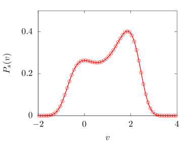
Figure 1: (Color online) Steady state probability distribution obtained from simulation (points), compared against the line drawn using the analytic form $P_{s}(v)={\cal N}\exp[-\chi(v)/D_{0}]$ with $\chi(v)=\frac{1}{2}(a+\gamma)v^{2}-\frac{b}{3}v^{3}+\frac{c}{4}v^{4}$ where $a=0$, $\gamma=1$, $b=2.4$, $c=1$ and $D_{0}=1$.

III.7 Probability distribution of entropy production

Let us now return to the coarse grained ABP model containing only velocity dependent forces, and consider a velocity dependent potential $\chi(v)=\frac{1}{2}(-a+\gamma)v^{2}-\frac{b}{3}v^{3}+\frac{c}{4}v^{4}$ such that the velocity dependent force $F(v)=g(v)+\xi(v)=-\partial_{v}\chi$. The corresponding Langevin equation of motion under this force $\dot{v}=\eta+g(v)+\xi(v)$ with $g(v)=(a-\gamma)v-cv^{3}$ and $\xi(v)=bv^{2}$. At steady state, the mean velocity has three solutions, $v=0,(b/2c)\pm\sqrt{b^{2}-4(-a+\gamma)c}/2c$. Among these solutions $v=0$ and $v=(b/2c)+\sqrt{b^{2}-4(-a+\gamma)c}/2c$ are stable fixed points and $v=(b/2c)-\sqrt{b^{2}-4(-a+\gamma)c}/2c$ is an unstable fixed point. The non-zero velocity stable fixed point gets viable for $b^{2}\geq 4c(-a+\gamma)$. In absence of external potential or force, the probability distribution is independent of position, obeying the FP equation $\partial_{t}P(v)=\partial_{v}[P\partial_{v}\chi+D_{0}\partial_{v}P]$. This has a steady state solution $P_{s}={\cal N}\exp[-\chi(v)/D_{0}]$ carrying non-zero dissipative current ${j}_{d}=g(v)P-D_{0}\partial_{v}P$.

From Eq.(16), the EP in the reservoir over time $\tau_{0}$ is expressed as $\Delta s_{r}=-\frac{1}{T}\left[\Delta Q+\frac{\Delta\psi}{\gamma}+\Delta Q_{em}\right]-\int^{\tau_{0}}dt\,\left[\frac{1}{T}\zeta(v)v+k_{B}\partial_{v}\xi(v)\right],$ where $\Delta Q$ is the heat absorbed over $\tau_{0}$, $\psi(v)=-\int dv\,\zeta(v)=av^{2}/2+cv^{4}/4$, $\Delta Q_{em}=\int^{\tau_{0}}dt\,\zeta(v)\,\xi(v)$. The simplest possible choice of such active velocity dependent force is $F(v)=bv^{2}-cv^{3}$, with $a=0$ and $b\geq\sqrt{4c\gamma}$ such that a real $v=(b/2c)+(b^{2}-4\gamma c)^{1/2}/2c$ stable fixed point in velocity is available. Note that the system EP over time $\tau_{0}$ is $\Delta s=k_{B}\ln[P_{s}(\tau)/P_{s}(0)]=\Delta\chi(v)/\gamma T$ where $\Delta\chi=\chi(v(\tau))-\chi(v(0))$, and $\chi(v)=\frac{1}{2}\gamma v^{2}-\frac{b}{3}v^{3}+\frac{c}{4}v^{4}$. Moreover, energy conservation, as discussed in Sec.III.3, implies $\Delta Q=\Delta E-\Delta Q_{m}$ as the work done due to external force is zero in the case considered here. Therefore, the total EP over time $\tau_{0}$ is $\Delta s_{t}=\Delta s+\Delta s_{r}=-(1/T)[\Delta E-\Delta Q_{m}+\Delta Q_{em}]-\int^{\tau_{0}}dt[\zeta(v)v/T+k_{B}\partial_{v}\xi(v)]-(1/\gamma T)(\Delta\psi-\Delta\chi)$. Using $a=0$, one obtains $\Delta E+(\Delta\psi-\Delta\chi)/\gamma=\Delta(bv^{3}/3\gamma)$, as $E=v^{2}/2$. Note that $-\Delta Q_{m}+\Delta Q_{em}+\int dt\zeta(v)vdt=\int dt[-vF(v)+\zeta(v)\xi(v)+\zeta(v)v]=\int dt\,[-v+\zeta(v)]\,\xi(v)$. Thus, one obtains

$$\Delta s_{t} = -\frac{1}{T}\left[\Delta\left(\frac{b}{3\gamma}v^{3}\right)+\int^{\tau_{0}}dt\{\zeta(v)-v\}\xi(v)\right]$$ (29)

$$-\int^{\tau_{0}}dt\,k_{B}\partial_{v}\xi(v).$$

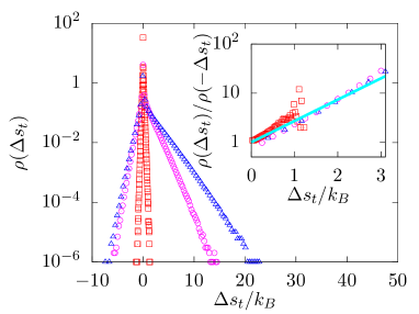
Figure 2: (Color online) Probability distribution of entropy production $\Delta s_{t}$ over time span $\tau_{0}$ = 16 ($\Box$), 64 ($\circ$), 128 ($\triangle$)  $\delta t$ plotted in linear-log scale. Inset: Ratio of probability distribution of positive and negative entropy production in linear-log scale. The solid line shows the function $\exp(\Delta s_{t}/k_{B})$. The deviation of data from this line is due to lack of statistics at large $\Delta s_{t}$.

We perform numerical integration of the Langevin dynamics of this ABP using Stratonovich discretization with time step $\delta t=10^{-4}\tau$, where $\tau=1/\gamma$, and parameters $D_{0}=1$, $k_{B}T=1$, $b=2.4$ and $c=1$. Figure 1 shows a plot of steady state velocity distribution obtained from the numerical simulation, showing good agreement with the analytic expression $P_{s}={\cal N}\exp[-\chi(v)/D_{0}]$. The distribution function has two maxima, at $v=0$ and $v=(b/2c)+\sqrt{b^{2}-4\gamma c}/2c$. On an average, the ABP moves towards the positive $x$ axis. From this simulation, we further obtain probability distribution of total stochastic EP, $\Delta s_{t}$, using the expression in Eq. 29, over different time spans $\tau_{0}$. The distribution function has a sharp peak at $\Delta s_{t}=0$, but gets broader for longer observation time $\tau_{0}$ (Fig.2). As shown in the inset of Fig. 2, the ratio of probability distribution of positive and negative EP shows good agreement with the detailed fluctuation theorem $\ln[\rho(\Delta s_{t})/\rho(-\Delta s_{t})]=\Delta s_{t}/k_{B}$.

IV Discussion

Models of self propelled particles in presence of non-linear velocity dependent force have been studied extensively in recent literature. We have shown earlier, if the velocity dependent force is odd under time reversal, the ABPs can not produce entropy unless coupled to conservative or non-conservative force Ganguly2013 ; Chaudhuri2014 . Given the self propulsion of the particles, even free ABPs should have produced entropy. In this paper, using an internal mechanism for generation of self propulsion, namely, in terms of an internal energy depot, we have shown, free ABPs of RH kind indeed produce entropy, albeit via the internal mechanism of producing self-propulsion, keeping the expression for EP in the velocity space unaltered. After integrating out the faster internal dofs, the self propulsion turns up as non-linear velocity dependent force in ABPs spatial motility.

We studied such coarse-grained models of ABPs, without explicit mechanism of self-propulsion, in the presence of a generic non-linear velocity dependent force, containing both odd and even functions of velocity. This leads to autonomous entropy production in velocity space. We have derived the expression for the total EP, independently, using the Fokker-Planck equation, and probability of time forward and time-reversed trajectories. Both the methods led to the same result. Note that the Jacobians in the path probability method, corresponding to the time forward and time reversed trajectories are not the same, unlike other simpler systems Narayan2004 ; Seifert2012 ; Seifert2008 . In fact, the ratio of these Jacobians contributes to the dependence of EP on the even part of the velocity dependent force under time reversal.

The total stochastic EP obeys fluctuation theorems. It is interesting to note that the EP in the reservoir has several excess contributions in addition to the Clausius entropy related to dissipated heat. This excess entropy shows two fundamentally new contributions with respect to earlier study involving force that is only an odd function of velocity Chaudhuri2014 . These are: (i) a velocity gradient of the even function of velocity, and (ii) cross-coupling of the odd and even functions of velocity. Using numerical simulations we have obtained probability distribution of the total EP and found good agreement with detailed fluctuation theorem. Note that the observation of excess EP, does not have any conflict with thermodynamic inequality due to Clausius, for systems out of equilibrium. In conclusion, each non-equilibrium dissipative mechanism not only adds to entropy independently, they often couple with each other to give rise to new terms in EP.

Appendix A Probability of a trajectory

The Langevin dynamics is described by

$$\dot{x} = v$$

$$\dot{v} = F(v)+\eta(t)+{\cal F}$$ (30)

where $F(v)=g(v)+\xi(v)$ with $g(v)=-\gamma v+\zeta(v)$, and ${\cal F}$ denotes the velocity-independent forces. The Gaussian white noise is characterized by $\langle\eta(t)\rangle=0$, $\langle\eta(t)\eta(0)\rangle=2D_{0}\delta(t)$ with $D_{0}=\gamma k_{B}T$. Discretizing the equation with $t=i\,\delta t$, using Stratonovich rule,

$$x_{i} = x_{i-1}+\frac{1}{2}(v_{i}+v_{i-1})\delta t$$

$$v_{i} = v_{i-1}+\frac{1}{2}\left[F(v_{i})+{\cal F}(x_{i})+F(v_{i-1})+{\cal F}(x_{i-1})\right]$$ (31)

$$+\eta_{i}\delta t.$$

The Gaussian random noise $\eta(t)$ follows the distribution $P(\eta_{i})=(\delta t/4\pi D_{0})\exp(-\delta t\eta_{i}^{2}/4D_{0})$ where $D_{0}=\gamma k_{B}T$. The transition probability over $i$-th segment of the trajectory $p^{+}_{i}\equiv P(x_{i},v_{i}|x_{i-1},v_{i-1})=J_{\eta_{i},v_{i}}\,\langle\delta(\dot{x}-v)\delta(\dot{v}-\{F(v)+{\cal F}\})\rangle$ leads to

$$p^{+}_{i}=J_{\eta_{i},v_{i}}\,\delta(\dot{x}-v)\sqrt{\frac{\delta t}{4\pi D_{0}}}e^{-\frac{\delta t}{4D_{0}}\left[\dot{v}-F(v)-{\cal F}\right]^{2}},$$ (32)

where

$$J_{\eta_{i},v_{i}} = {\rm det}\left(\frac{\partial\eta_{i}}{\partial v_{i}}\right)=\frac{1}{\delta t}\left(1-\frac{\delta t}{2}\partial_{v_{i}}F(v_{i})\right)$$ (33)

$$= \frac{1}{\delta t}\left(1-\frac{\delta t}{2}\partial_{v_{i}}[g(v_{i})+\xi(v_{i})]\right)$$

using Eq.(31). The probability associated with a full trajectory is ${\cal P}^{+}=\prod_{i}p^{+}_{i}$.

References

- (1) T. Vicsek and A. Zafeiris, Physics Reports 517, 71 (2012).
- (2) T. Vicsek, A. Czirók, E. Ben-Jacob, I. Cohen, and O. Shochet, Physical Review Letters 75, 1226 (1995).
- (3) J. R. Howse, R. A. L. Jones, A. J. Ryan, T. Gough, R. Vafabakhsh, and R. Golestanian, Physical Review Letters 99, 048102 (2007).
- (4) X. Zheng, B. ten Hagen, A. Kaiser, M. Wu, H. Cui, Z. Silber-Li, and H. Löwen, Physical Review E 88, 032304 (2013).
- (5) A. Nourhani, Y.-M. Byun, P. E. Lammert, A. Borhan, and V. H. Crespi, Physical Review E 88, 062317 (2013).
- (6) K. Feitosa and N. Menon, Physical Review Letters 92, 164301 (2004).
- (7) S. Joubaud, D. Lohse, and D. van der Meer, Physical Review Letters 108, 210604 (2012).
- (8) N. Kumar, S. Ramaswamy, and A. K. Sood, Physical Review Letters 106, 118001 (2011).
- (9) P. Romanczuk, M. Bär, W. Ebeling, B. Lindner, and L. Schimansky-Geier, The European Physical Journal Special Topics 202, 1 (2012).
- (10) M. Badoual, F. Jülicher, and J. Prost, Proceedings of the National Academy of Sciences of the United States of America 99, 6696 (2002).
- (11) F. Jülicher and J. Prost, Physical Review Letters 75, 2618 (1995).
- (12) F. Schweitzer, W. Ebeling, and B. Tilch, Physical Review Letters 80, 5044 (1998).
- (13) Y. Zhang, C. K. Kim, and K. J. B. Lee, New J. Phys. 10, 103018 (2008).
- (14) K. Sekimoto, Progress of Theoretical Physics Supplement 130, 17 (1998).
- (15) C. Bustamante, J. Liphardt, and F. Ritort, Physics Today 58, 43 (2005).
- (16) U. Seifert, Rep. Prog. Phys. 75, 126001 (2012).
- (17) C. Jarzynski, Annu. Rev. Condens. Matter Phys. 2, 329 (2011).
- (18) C. Jarzynski, Phys. Rev. Lett. 78, 2690 (1997).
- (19) G. E. Crooks, Physical Review E 60, 2721 (1999).
- (20) G. M. Wang, E. M. Sevick, E. Mittag, D. J. Searles, and D. J. Evans, Physical Review Letters 89, 050601 (2002).
- (21) J. Liphardt, S. Dumont, S. B. Smith, I. Tinoco, and C. Bustamante, Science 296, 1832 (2002).
- (22) O. Narayan and A. Dhar, J. Phys. A: Math. Gen. 37, 63 (2004).
- (23) J. Kurchan, Journal of Statistical Mechanics: Theory and Experiment 2007, P07005 (2007).
- (24) D. J. Evans, E. G. D. Cohen, and G. P. Morriss, Physical Review Letters 71, 2401 (1993).
- (25) G. Gallavotti and E. G. D. Cohen, Physical Review Letters 74, 2694 (1995).
- (26) J. L. Lebowitz and H. Spohn, Journal of Statistical Physics 95, 333 (1999).
- (27) U. Seifert, Physical Review Letters 95, 040602 (2005).
- (28) U. Seifert, in Soft Matter. From Synthetic to Biological Materials, LectureNotes of the 39th Spring School 2008, edited by J. K. G. Dhont, G. Gompper, G. Nägele, D. Richter, and R. G. Winkler (Forschungszentrum Jülich, Jülich, 2008), pp. 1–30.
- (29) A. Gnoli, A. Petri, F. Dalton, G. Pontuale, G. Gradenigo, A. Sarracino, and A. Puglisi, Phys. Rev. Lett. 110, 120601 (2013).
- (30) A. Sarracino, Physical Review E 88, 052124 (2013).
- (31) L. Cerino and a. Puglisi, EPL (Europhysics Lett. 111, 40012 (2015).
- (32) A. Puglisi, S. Pigolotti, L. Rondoni, and A. Vulpiani, J. Stat. Mech. Theory Exp. 2010, P05015 (2010).
- (33) A. Crisanti, A. Puglisi, and D. Villamaina, Phys. Rev. E 85, 061127 (2012).
- (34) J. Mehl, B. Lander, C. Bechinger, V. Blickle, and U. Seifert, Phys. Rev. Lett. 108, 220601 (2012).
- (35) C. Jia, Phys. Rev. E 93, 052149 (2016).
- (36) V. Blickle, T. Speck, L. Helden, U. Seifert, and C. Bechinger, Physical Review Letters 96, 070603 (2006).
- (37) T. Speck, V. Blickle, C. Bechinger, and U. Seifert, Euro. Phys. Lett. 79, 30002 (2007).
- (38) D. Collin, F. Ritort, C. Jarzynski, S. B. Smith, I. Tinoco, and C. Bustamante, Nature 437, 231 (2005).
- (39) U. Seifert, The European Physical Journal E 34, 26 (2011).
- (40) D. Lacoste and K. Mallick, Biological Physics 60, 61 (2011).
- (41) D. Lacoste and K. Mallick, Phys. Rev. E 80, 021923 (2009).
- (42) K. Hayashi, H. Ueno, R. Iino, and H. Noji, Physical Review Letters 104, 218103 (2010).
- (43) K. Hayashi, M. Tanigawara, and J.-i. Kishikawa, Biophysics 8, 67 (2012).
- (44) C. Ganguly and D. Chaudhuri, Physical Review E 88, 032102 (2013).
- (45) D. Chaudhuri, Phys. Rev. E 90, 022131 (2014).
- (46) S. Bandopadhyay, D. Chaudhuri, and A. M. Jayannavar, Phys. Rev. E 92, 032143 (2015).
- (47) S. Bandopadhyay, D. Chaudhuri, and A. M. Jayannavar, Journal of Statistical Mechanics: Theory and Experiment 2015, P11002 (2015).
- (48) D. Chaudhuri, under preparation.