Dynamics of Warm Chaplygin Gas Inflationary Models With Quartic Potential

Abstract

Warm inflationary universe models in the context of generalized chaplygin gas, modified chaplygin gas, generalized cosmic chaplygin gas are being studied. The dissipative coefficient of the form $\Gamma\propto T$, weak and strong dissipative regimes are being considered. We use quartic potential $\frac{\lambda_{*}\phi^{4}}{4}$, which is ruled out by current data in cold inflation but in our models it is analyzed that it is in agreement with the WMAP$9$ and latest Planck data. In these scenarios, the power spectrum, spectral index, and tensor to scalar ratio are being examined under the slow roll approximation. We show the dependence of tensor scalar ratio $r$ on spectral index $n_{s}$ and observe that the range of tensor scalar ratio is $r<0.05$ in generalized chaplygin gas, $r<0.15$ in modified chaplygin gas, and $r<0.12$ in generalized cosmic chaplygin gas models. Our results are in agreement with recent observational data like WMAP$9$ and latest Planck data.

Keywords: Warm Inflation; Chaplygin gas models; Quartic potential; Inflationary Parameters.

1 Introduction

It is well known that inflation presents most compelling solution of many problems of big bang model, namely the horizon, flatness, homogeneity and monopoles problems [1]. The most fascinating feature of inflationary universe model is that it interprets the origin of observed anisotropy in the cosmic microwave background radiations, and also the distribution of large scale structures [2]. But some questions arises in theory of inflation, one of them is how to end this inflationary epoch and enter in bing bang phase. Warm inflation provides a possible solution to this problem. Standard inflation known as cold inflation, has two regimes slow roll and reheating. In slow roll limits, universe expands as potential energy dominates the kinetic energy and interaction of inflation (scalar field) with other fields become negligible. In reheating epoch, kinetic energy is comparable to potential energy and inflation oscillates around the minimum of its potential while losing its energy to massless particles. After reheating, the universe is filled with radiation.

Warm inflation provides a mechanism in which reheating is avoided. During the warm inflationary period, dissipative effects are important, so that radiation production takes place at the same time as inflationary expansion. A strong regime in warm inflation is that in which damping effects on inflation dynamics of radiation field are strong, these dissipating effects originates from a friction term which describe the physical process of decay of inflation field into a thermal bath due to its interaction with other field. Decay of remaining inflationary field or dominant radiation create the mater component of universe. Warm inflation come to an end when universe heats up and become radiation dominated and gets connected with the big bang scenario [3, 23]. In standard inflation density perturbations are generated due to quantum fluctuations associated to the inflation scalar field, which are necessary for the large scale structure formation at the late time in the evolution of the universe. However, in warm inflation, thermal fluctuations instead of quantum fluctuations become a source of density perturbations [5, 6].

Monerat et al. [11] studied cosmology of the early universe and the initial condition for inflation in a model with radiation and chaplygin gas (CG). Antonella et al. [15] discussed warm inflation on brane. Del campo and Herrera [13] considered warm inflationary model with generalized chaplygin gas (GCG), they used a standard scalar field and dissipation coefficient of the form $\Gamma\propto\phi^{n}$ and then develop the model with chaotic potential. Setare and Kamali investigated warm tachyon inflation by assuming intermediate [14] and logamediate scenario [17]. Bastero-Gill et al. obtained the expressions for the dissipation coefficient in supersymmetric (SUSY) models in [16]. This result provides possibilities for realization of warm inflation in SUSY field theories.

Herrera et al. [18] studied intermediate inflation in the context of GCG using standard and tachyon scalar field. Same authors also dealt with dissipation coefficient $\Gamma=c\frac{T^{m}}{\phi^{m-1}}$ in the context of warm intermediate and logamediate inflationary models [19]. They also studied warm inflation in loop quantum cosmology with the same dissipative coefficient [20]. Bastero-Gill et al. in [21] have also explored inflation by assuming the quartic potential. Sharif and Saleem [22] studied inflationary models with generalized cosmic chaplygin gas (GCCG). Setare and Kamali analyzed warm viscous inflation on brane in [23]. They have also considered a generalized de-sitter scale factor including single scalar field and studied q-inflation in the context of warm inflation with two forms of damping term [24]. Panotopoulos and Videla [25] investigated the quartic potential model in the framework of warm inflation by using a decay rate proportional to temperature and showed that it is compatible with latest observational data. We extend this work with the inclusion of chaplygin gas (CG) models.

The goal of present work is to investigate the realization of warm quartic inflationary model in the context of CG models. This paper is organized as follows: Next section deals with basic background equations of warm inflationary scenario. In section 3, we construct models with (GCG), (MCG) and (GCCG) by using a quartic potential. In the last section, we summarized our results.

2 Basic Inflationary Scenario

We start by using Friedmann Robertson Walker (FRW) metric and consider a spatially flat universe which contains a self interacting inflation field $\phi$ and radiation field, where $V(\phi)$ is scalar potential, $\rho_{\phi}$ and $\rho_{\gamma}$ are energy densities of inflation field and radiation field respectively, then write down a modified Friedmann equation of the form

$$H^{2}=\frac{1}{3M_{p}^{2}}(\rho_{\phi}+\rho_{\gamma}),$$ (1)

where $M_{p}=\frac{1}{\sqrt{8\pi G}}$ is reduced planck mass, and $\rho_{\phi}=\frac{\dot{\phi}^{2}}{2}+V(\phi)$, $P_{\phi}=\frac{\dot{\phi}^{2}}{2}-V(\phi)$ are the energy densities and potential of scalar field, respectively. Energy-momentum conservation leads to the following equations [3, 23]

$$\dot{\rho_{\phi}}+3H(\rho_{\phi}+P_{\phi})=-\Gamma\dot{\phi}^{2},\quad\dot{\rho_{\gamma}}+4H(\rho_{\gamma})=\Gamma\dot{\phi}^{2}.$$ (2)

Dynamics of warm inflation is described by adding a friction term in the equation of motion given by

$$\ddot{\phi}+(3H+\Gamma)\dot{\phi}+V^{\prime}=0,$$ (3)

$\Gamma$ is the dissipation coefficient. During the inflation era, $\Gamma$ is responsible for the decay of scalar field into radiation, this decay rate can be a function of scalar field or temperature or depend on both $\Gamma(T,\phi)$ or simply a constant. During warm inflation production of radiation is quasi-stable, i.e. $\dot{\rho_{\gamma}}\ll 4H\rho_{\gamma}$ and $\dot{\rho_{\gamma}}\ll\Gamma\dot{\phi}^{2}$ [3, 23, 5, 7, 8, 9], the energy density associated with scalar field dominates over the energy density of radiation field, i.e. $\rho_{\phi}\gg\rho_{\gamma}$. Assuming the set of slow roll conditions, i.e. $\dot{\phi}^{2}\ll V(\phi)$ and $\ddot{\phi}\ll(3H+\Gamma)\dot{\phi}$ [3, 23], then the equations of motion reduces to

$$3H(1+R)\dot{\phi}\simeq-V^{\prime},\quad 4H\rho_{\gamma}\simeq\Gamma\dot{\phi}^{2},$$ (4)

here dot mean derivatives with respect to time and $V^{\prime}=\frac{\partial V}{\partial\phi}$. A dissipation coefficient is basic quantity, which has been calculated from first principles in the context of supersymmetry. In these models, there is a scalar field with multiplets of heavy and light fields that make it possible to obtain several expression for dissipation coefficient. A general form for $\Gamma$ can be written as [26, 27]

$$\Gamma=b\frac{T^{m}}{\phi^{m-1}},$$

where $b$ is associated to dissipative microscopic dynamics and exponent $m$ is integer. In literature different cases have been studied for the different values of $m$, in special case $m=1$, i.e. $\Gamma\propto T$ represent high temperature SUSY case, for the value $m=0$ i.e. $\Gamma\propto\phi$ corresponds to an exponentially decaying propagator in the high temperature SUSY model, for $m=-1$ i.e. $\Gamma\propto\frac{\phi^{2}}{T}$, we have agreement with non-SUSY case [28, 29]. We introduce a parameter $R=\frac{\Gamma}{3H}$ which is the relative strength of thermal damping compared to the expansion damping. In warm inflation, we can assume two possible scenarios, one is weak dissipative regime defined as $R\ll 1$, in which Hubble damping is still the dominant term, and the other one is strong dissipative regime defined as $R\gg 1$, the $\Gamma$ controls damped evolution of the inflation field in it.

Moreover, the thermalization energy density of radiation field can be written as $\rho_{\gamma}=CT^{4}$, where constant $C=\pi^{2}g_{*}/30$, and $g_{*}$ denotes the number of relativistic degrees of freedom, in a Minimal Supersymmetric Standard Model (MSSM), $g_{*}=228.75$ and $C\simeq 70$ [5]. Using Eq.(4) and $\rho_{\gamma}\propto T^{4}$ temperature becomes

$$T=\bigg{[}\frac{\Gamma V^{\prime 2}}{6^{2}CH^{3}(1+R)^{2}}\bigg{]}^{\frac{1}{4}}.$$ (5)

Slow roll parameters of warm inflation are given by [5]

$$\epsilon=\frac{-\dot{H}}{H^{2}},\quad\eta=\frac{-\ddot{H}}{H\dot{H}},\quad\beta=-\frac{1}{H}\frac{d}{dt}(ln\Gamma).$$

In warm inflation, slow roll conditions are expressed as $\epsilon\ll 1+R$, $\eta\ll 1+R$, $\beta\ll 1+R$. On the other hand, the number of e-folds is calculated by using the standard formula

$$N=\int_{t_{*}}^{t_{end}}Hdt.$$ (6)

Here, $t_{*}$ and $t_{end}$ denotes the time when inflation starts and comes to an end respectively.

Next, we discuss the perturbation parameters for the current scenario by assuming CG models. The perturbation parameters of the warm inflation are obtained in [5]. The amplitude of the power spectrum of the curvature perturbation is given by

$$P_{R}=\bigg{(}\frac{\pi}{4}\bigg{)}^{\frac{1}{2}}\frac{H^{\frac{5}{2}}\Gamma^{\frac{1}{2}}T}{\dot{\phi}^{2}},$$ (7)

we can calculate the scalar spectral index $n_{s}$ by using $n_{s}=1+\frac{dP_{R}}{dlnk}$ which is equivalent to

$$n_{s}=1-\frac{9\epsilon}{4}+\frac{3\eta}{2}-\frac{9\beta}{4}.$$ (8)

However tensor to scalar ratio turns out to be [24]

$$r=\frac{32G\dot{\phi}^{2}}{\Gamma^{\frac{1}{2}}\pi^{\frac{3}{2}}TH^{\frac{1}{2}}}.$$ (9)

In the following, we take a standard scalar field and $\Gamma\propto T$ to study how these conditions effects the inflationary dynamics for quartic potential.

3 Chaplygin Inflationary Models With Quartic Potential

We consider a quartic potential $V(\phi)=\frac{\lambda_{*}\phi^{4}}{4}$ which is a simple Higgs potential developed in particle physics theories [10]. In the following work, we assume an inflation decay rate $\Gamma=bT$ and quartic potential in warm inflation models with chaplygin gas.

3.1 Generalized Chaplygin Gas

The CG is considered to be an alternative description of accelerating expansion and it has a connection with string theory. CG emerges as an effective fluid of generalized D-brane in a $(d+1,1)$ space time where the action can be written as a generalized born-infield action [30]. Kammshchick [31] considered FRW universe composed of CG and showed that universe is in agreement with current observation of cosmic acceleration. Its extended form is GCG whose equation of state (EoS) is as follows

$$P_{gcg}=-\frac{A}{\rho_{gcg}^{\lambda}},$$

where $P_{gcg}$ and $\rho_{gcg}$ denote the pressure and energy density respectively and $0<\lambda\leq 1$, and A is the positive constant. The energy density of GCG can be obtained by using equation of continuity and given by

$$\rho_{gcg}=\bigg{(}A+\frac{B}{a^{3(1+\lambda)}}\bigg{)}^{\frac{1}{1+\lambda}},$$ (10)

where $B$ is a positive integration constant and $a$ is scale factor. We start with the modified Friedmann equation of the form

$$H^{2}=\frac{1}{3M_{p}^{2}}\bigg{(}\big{(}A+\rho_{\phi}^{1+\lambda}\big{)}^{\frac{1}{1+\lambda}}+\rho_{\gamma}\bigg{)}.$$ (11)

This modification is possible due to an extrapolation of Eq.(10) so that

$$\rho_{gcg}=\big{(}A+\rho_{m}^{1+\lambda}\big{)}^{\frac{1}{1+\lambda}}\rightarrow\big{(}A+\rho_{\phi}^{1+\lambda}\big{)}^{\frac{1}{1+\lambda}},$$ (12)

where $\rho_{m}$ denotes the matter energy density. During the inflation era, energy density of scalar field dominates the energy density of radiation field, i.e., $\rho_{\phi}\gg\rho_{\gamma}$, and it is of the order of potential i.e. $\rho_{\phi}\sim V$. For simplicity, we take $\lambda=1$ for which the Friedmann equation takes the form

$$H^{2}=\frac{1}{3M_{p}^{2}}\sqrt{A+\rho_{\phi}^{2}}\sim\frac{1}{3M_{p}^{2}}\sqrt{A+V^{2}}.$$ (13)

3.1.1 Weak Dissipative Regime

Here, we consider weak dissipative regime where $R\ll 1$, the Friedmann and Klein-Gordon equations take the standard form under slow-roll approximation. By taking $\Gamma=bT$, the temperature of radiation field becomes

$$T=\bigg{(}\frac{bV^{\prime 2}}{6^{2}CH^{3}}\bigg{)}^{\frac{1}{3}}.$$

For weak dissipative regime, the slow roll parameters are as follows

$$\epsilon = \frac{M_{p}^{2}VV^{\prime 2}}{2(A+V^{2})^{\frac{3}{2}}},\quad\eta=\frac{M_{p}^{2}}{(A+V^{2})^{\frac{1}{2}}}\bigg{(}V^{\prime\prime}+\frac{V^{\prime 2}}{V}-\frac{3VV^{\prime 2}}{2(A+V^{2})}\bigg{)},$$

$$\beta = M_{p}^{2}\bigg{(}\frac{4V^{\prime\prime}(A+V^{2})-3V^{\prime 2}V}{6(A+V^{2})^{\frac{3}{2}}}\bigg{)}.$$

By using the Eq.(6), the number of e-folds become

$$N=\frac{1}{M_{p}^{2}}\int_{\phi_{end}}^{\phi_{*}}\frac{\sqrt{A+V^{2}}}{V^{\prime}}d\phi.$$

Amplitude of power spectrum given in Eq.(7) takes the form

$$P_{R} = \bigg{(}\frac{81\pi b^{2}}{12^{2}CV^{\prime 2}}\bigg{)}^{\frac{1}{2}}\bigg{(}\frac{\sqrt{A+V^{2}}}{3M_{p}^{2}}\bigg{)}^{\frac{3}{2}}.$$ (14)

By inserting the values in Eq.(8), scalar spectral index turns out to be

$$n_{s}-1 = \frac{3M_{p}^{2}}{2(A+V^{2})^{\frac{1}{2}}}\bigg{(}\frac{-9VV^{\prime 2}}{4(A+V^{2})}-\frac{3}{2}\bigg{(}\frac{4V^{\prime\prime}(A+V^{2})-3V^{\prime 2}V}{6(A+V^{2})}\bigg{)}$$

$$+V^{\prime\prime}+\frac{V^{\prime 2}}{V}\bigg{)}.$$

The tensor to scalar ratio given in Eq.(9) become

$$r=\frac{192G\sqrt{3CM_{p}^{2}}V^{\prime}}{9b\pi^{\frac{3}{2}}(A+V^{2})^{\frac{1}{4}}}.$$ (16)

We use $V=\frac{\lambda_{*}\phi^{4}}{4}$ and $V^{\prime}=\lambda_{*}\phi^{3}$ to express $r$ and $n_{s}$ as function of $\phi$,

$$n_{s}-1 = \frac{12M_{p}^{2}}{2(16A+\lambda^{2}_{*}\phi^{8})^{\frac{1}{2}}}\bigg{(}\frac{-6\lambda^{3}_{*}\phi^{10}}{16A+\lambda^{2}_{*}\phi^{8}}+4\lambda_{*}\phi^{2}\bigg{)},\quad r=\frac{384G\sqrt{3CM_{p}^{2}}\lambda_{*}\phi^{3}}{9b\pi^{\frac{3}{2}}(16A+\lambda^{2}_{*}\phi^{8})^{\frac{1}{4}}}.$$

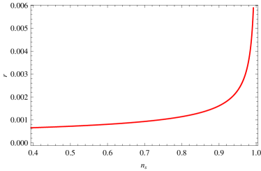
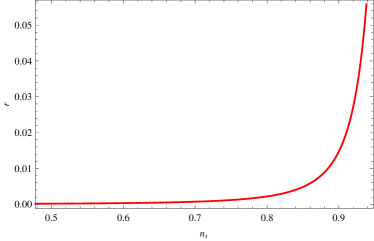
Figure 1: Plot of tensor-scalar ratio $r$ versus scalar spectral index $n_{s}$ for GCG model in weak dissipative regime (left panel) and strong dissipative regime (right panel)

3.1.2 Strong Dissipative Regime

Now we consider a strong dissipative regime where $R\gg 1$, under the slow roll approximation, the temperature is given as

$$T=\bigg{(}\frac{V^{\prime 2}}{4bCH}\bigg{)}^{\frac{1}{5}}.$$

For strong regime, the slow roll parameters leads to

$$\epsilon = \frac{M_{p}^{2}VV^{\prime 2}}{2R(A+V^{2})^{\frac{3}{2}}},$$

$$\eta = \frac{M_{p}^{2}}{R(A+V^{2})^{\frac{1}{2}}}\bigg{(}V^{\prime\prime}+\frac{V^{\prime 2}}{V}-\frac{3VV^{\prime 2}}{2(A+V^{2})}\bigg{)},$$

$$\beta = \frac{1}{R}M_{p}^{2}\bigg{(}\frac{2V^{\prime\prime}(A+V^{2})-V^{\prime 2}V}{5(A+V^{2})^{\frac{3}{2}}}\bigg{)}.$$

The expression of number of e-folds takes the following form

$$N=\frac{1}{M_{p}^{2}}\int_{\phi_{end}}^{\phi_{*}}\frac{\sqrt{A+V^{2}}}{V^{\prime}}Rd\phi.$$

In the similar way, we can obtain the amplitude of power spectrum, scalar spectral index and tensor to scalar ratio as follows

$$P_{R} = \big{(}\frac{\pi}{4}\big{)}^{\frac{1}{2}}\frac{b^{\frac{9}{5}}}{V^{\prime\frac{3}{5}}(4C)^{\frac{7}{10}}}\bigg{(}\frac{\sqrt{A+V^{2}}}{3M_{p}^{2}}\bigg{)}^{\frac{9}{10}},$$ (17)

$$n_{s}-1 = \bigg{(}\frac{3(4C)^{\frac{1}{5}}}{b^{\frac{4}{5}}V^{\prime\frac{2}{5}}}\bigg{)}\frac{(3M_{p}^{2})^{\frac{2}{5}}}{2(A+V^{2})^{\frac{1}{5}}}\bigg{(}V^{\prime\prime}+\frac{V^{\prime 2}}{V}-\frac{9VV^{\prime 2}}{4(A+V^{2})}$$

$$-\frac{3}{2}\bigg{(}\frac{2V^{\prime\prime}(A+V^{2})-V^{\prime 2}V}{5(A+V^{2})}\bigg{)}\bigg{)},$$

$$r = \frac{32G(4C)^{\frac{7}{10}}V^{\prime\frac{3}{5}}}{b^{\frac{9}{5}}\pi^{\frac{3}{2}}}\bigg{(}\frac{\sqrt{A+V^{2}}}{3M_{p}^{2}}\bigg{)}^{\frac{1}{10}}.$$ (19)

In terms of scalar field, $r$ and $n_{s}$ turn out to be

$$n_{s}-1 = \bigg{(}\frac{3(4C)^{\frac{1}{5}}}{b^{\frac{4}{5}}(\lambda_{*}\phi^{3})^{\frac{2}{5}}}\bigg{)}\frac{(3M_{p}^{2})^{\frac{2}{5}}}{10(16A+\lambda^{2}_{*}\phi^{8})^{\frac{1}{5}}}\bigg{(}\frac{-39\lambda^{3}_{*}\phi^{10}}{16A+\lambda^{2}_{*}\phi^{8}}+26\lambda_{*}\phi^{2}\bigg{)},$$ (20)

$$r = \frac{32G(4C)^{\frac{7}{10}}(\lambda_{*}\phi^{3})^{\frac{3}{5}}}{b^{\frac{9}{5}}\pi^{\frac{3}{2}}}\bigg{(}\frac{\sqrt{16A+\lambda_{*}^{2}\phi^{8}}}{12M_{p}^{2}}\bigg{)}^{\frac{1}{10}}.$$ (21)

We plot the $r$ versus $n_{s}$ for GCG models in Figure 1 for weak (left panel) and strong dissipative regimes (right panel), respectively. However, the parameters appearing in the model have following values $M_{p}=1$, $\lambda_{*}=10^{-10}$, $A=10^{-45}$, $b=0.3$. The trajectories in the Figure 1 show the increasing behavior of $r$ with respect to $n_{s}$. It can be noted that in weak dissipative regime (left panel of Figure 1) that the range of tensor-to-scalar ration becomes $r<0.006$ for $0.4<n_{s}<1$. However, it is $r=0.05$ corresponding to $n_{s}=0.96$ for strong dissipative regime (left panel of Figure 1). It is observed that WMAP$9$ [32] provides the value of tensor scalar ratio as $r<0.13$ and spectral index is measured to be $n_{s}=0.972\pm 0.013$. According to Planck data, $r<0.11$ and $n_{s}=0.968\pm 0.006$ [33]. In view of these observations, our results for GCG model are compatible with observational data [32, 33].

3.2 Modified Chaplygin Gas

The MCG has a equation of state as follows [34]

$$P_{mcg}=\mu\rho_{mcg}-\frac{\nu}{\rho_{mcg}^{\lambda}},$$

where $P_{mcg}$ and $\rho_{mcg}$ denote the pressure and energy density respectively and $0\leq\lambda\leq 1$, $\mu$, $\nu$ are positive constants. We use energy conservation equation and express the density of MCG in this form

$$\rho_{mcg}=\bigg{(}A+\frac{c}{a^{3(1+\lambda)(1+\mu)}}\bigg{)}^{\frac{1}{1+\lambda}},$$ (22)

where $c$ is constant of integration and $A=\frac{\nu}{1+\mu}$ . We start with the modified Friedmann equation of the form

$$H^{2}=\frac{1}{3M_{p}^{2}}\bigg{(}\big{(}A+\rho_{\phi}^{(1+\lambda)(1+\mu)}\big{)}^{\frac{1}{1+\lambda}}+\rho_{\gamma}\bigg{)},$$ (23)

this modification is possible only due to an extrapolation of Eq.(22) so that

$$\rho_{mcg}=\big{(}A+\rho_{m}^{(1+\lambda)(1+\mu)}\big{)}^{\frac{1}{1+\lambda}}\rightarrow\big{(}A+\rho_{\phi}^{(1+\lambda)(1+\mu)}\big{)}^{\frac{1}{1+\lambda}},$$ (24)

where $\rho_{m}$ denotes the matter energy density, and hence the Friedmann equation takes the form

$$H^{2}=\frac{1}{3M_{p}^{2}}(A+\rho_{\phi}^{(1+\lambda)(1+\mu)})^{\frac{1}{1+\lambda}}\sim\frac{1}{3M_{p}^{2}}(A+V^{(1+\lambda)(1+\mu)})^{\frac{1}{1+\lambda}}.$$ (25)

3.2.1 Weak Dissipative Regime

For weak dissipative regime the temperature remains same as given in GCG case. However, the slow roll parameters takes the following form

$$\epsilon = \frac{M_{p}^{2}(1+\mu)V^{(1+\lambda)(1+\mu)-1}V^{\prime 2}}{2(A+V^{(1+\lambda)(1+\mu)})^{\frac{2+\lambda}{1+\lambda}}},$$

$$\eta = \frac{M_{p}^{2}}{(A+V^{(1+\lambda)(1+\mu)})^{\frac{1}{1+\lambda}}}\bigg{(}2V^{\prime\prime}+\frac{V^{\prime 2}((1+\lambda)(1+\mu)-1)}{V}$$

$$-\frac{V^{(1+\lambda)(1+\mu)-1}V^{\prime 2}(1+\lambda)(1+\mu)}{(A+V^{(1+\lambda)(1+\mu)})}\bigg{)},$$

$$\beta = M_{p}^{2}\bigg{(}\frac{4(A+V^{(1+\lambda)(1+\mu)})V^{\prime\prime}-3(1+\mu)V^{\prime 2}V^{(1+\lambda)(1+\mu)-1}}{6(A+V^{(1+\lambda)(1+\mu)})^{\frac{2+\lambda}{1+\lambda}}}\bigg{)}.$$

The number of e-folds are obtained as

$$N=\frac{1}{M_{p}^{2}}\int_{\phi_{end}}^{\phi_{*}}\frac{(A+V^{(1+\lambda)(1+\mu)})^{\frac{1}{1+\lambda}}}{V^{\prime}}d\phi.$$

Other perturbed parameters turns out to be

$$P_{R} = \bigg{(}\frac{81\pi b^{2}}{12^{2}CV^{\prime 2}}\bigg{)}^{\frac{1}{2}}\bigg{(}\frac{(A+V^{(1+\lambda)(1+\mu)})^{\frac{1}{1+\lambda}}}{3M_{p}^{2}}\bigg{)}^{\frac{3}{2}},$$ (26)

$$n_{s}-1 = \frac{3M_{p}^{2}}{2(A+V^{(1+\lambda)(1+\mu)})^{\frac{1}{1+\lambda}}}\bigg{(}\frac{V^{\prime 2}((1+\lambda)(1+\mu)-1)}{V}$$

$$-\frac{V^{(1+\lambda)(1+\mu)-1}V^{\prime 2}}{(A+V^{(1+\lambda)(1+\mu)})}\big{(}\frac{3}{4}(1+\mu)+(1+\lambda)(1+\mu)\big{)}+2V^{\prime\prime}$$

$$-\frac{3}{2}\big{(}\frac{4(A+V^{(1+\lambda)(1+\mu)})V^{\prime\prime}-3(1+\mu)V^{\prime 2}V^{(1+\lambda)(1+\mu)-1}}{6(A+V^{(1+\lambda)(1+\mu)})}\big{)}\bigg{)},$$

$$r = \frac{192G\sqrt{3CM_{p}^{2}}V^{\prime}}{9b\pi^{\frac{3}{2}}(A+V^{(1+\lambda)(1+\mu)})^{\frac{1}{2(1+\lambda)}}}.$$ (28)

By using a quartic potential $r$ and $n_{s}$ are expressed as function of $\phi$,

$$n_{s}-1 = \frac{3M_{p}^{2}}{2(A+(0.25\lambda_{*}\phi^{4})^{(1+\lambda)(1+\mu)})^{\frac{1}{1+\lambda}}}\bigg{(}\lambda_{*}\phi^{2}((1+\lambda)(1+\mu)-1)$$

$$-\frac{(0.25\lambda_{*}\phi^{4})^{(1+\lambda)(1+\mu)-1}\lambda_{*}^{2}\phi^{6}}{(A+(0.25\lambda_{*}\phi^{4})^{(1+\lambda)(1+\mu)})}\big{(}\frac{3}{4}(1+\mu)+(1+\lambda)(1+\mu)\big{)}+6\lambda_{*}\phi^{2}$$

$$-\frac{3}{12(A+(0.25\lambda_{*}\phi^{4})^{(1+\lambda)(1+\mu)})}\big{(}4(A+(0.25\lambda_{*}\phi^{4})^{(1+\lambda)(1+\mu)})\lambda_{*}\phi^{2}$$

$$-3(1+\mu)\lambda_{*}^{2}\phi^{6}(0.25\lambda_{*}\phi^{4})^{(1+\lambda)(1+\mu)-1}\big{)}\bigg{)},$$

$$r = \frac{192G\sqrt{3CM_{p}^{2}}\lambda_{*}\phi^{3}}{9b\pi^{\frac{3}{2}}(A+(0.25\lambda_{*}\phi^{4})^{(1+\lambda)(1+\mu)})^{\frac{1}{2(1+\lambda)}}}.$$ (30)

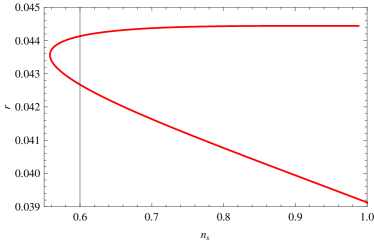
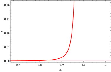
Figure 2: Plot of tensor-scalar ratio $r$ versus scalar spectral index $n_{s}$ for MCG model in weak dissipative regime (left panel) and strong dissipative regime (right panel)

3.2.2 Strong Dissipative Regime

Here, we mention that the temperature remains same as obtained in GCG case for strong regime. However, the slow roll parameters take the form

$$\epsilon = \frac{M_{p}^{2}(1+\mu)V^{(1+\lambda)(1+\mu)-1}V^{\prime 2}}{2R(A+V^{(1+\lambda)(1+\mu)})^{\frac{2+\lambda}{1+\lambda}}},$$

$$\eta = \frac{M_{p}^{2}}{R(A+V^{(1+\lambda)(1+\mu)})^{\frac{1}{1+\lambda}}}\bigg{(}2V^{\prime\prime}+\frac{V^{\prime 2}((1+\lambda)(1+\mu)-1)}{V}$$

$$-\frac{V^{(1+\lambda)(1+\mu)-1}V^{\prime 2}(1+\lambda)(1+\mu)}{(A+V^{(1+\lambda)(1+\mu)})}\bigg{)},$$

$$\beta = \frac{1}{R}M_{p}^{2}\bigg{(}\frac{4(A+V^{(1+\lambda)(1+\mu)})V^{\prime\prime}-(1+\mu)V^{\prime 2}V^{(1+\lambda)(1+\mu)-1}}{10(A+V^{(1+\lambda)(1+\mu)})^{\frac{2+\lambda}{1+\lambda}}}\bigg{)}.$$

The number of e-folds is given by

$$N=\frac{1}{M_{p}^{2}}\int_{\phi_{end}}^{\phi_{*}}\frac{(A+V^{(1+\lambda)(1+\mu)})^{\frac{1}{1+\lambda}}}{V^{\prime}}Rd\phi.$$

Other perturbed quantities lead to

$$P_{R} = \big{(}\frac{\pi}{4}\big{)}^{\frac{1}{2}}\frac{b^{\frac{9}{5}}}{V^{\prime\frac{3}{5}}(4C)^{\frac{7}{10}}}\bigg{(}\frac{(A+V^{(1+\lambda)(1+\mu)})^{\frac{1}{1+\lambda}}}{3M_{p}^{2}}\bigg{)}^{\frac{9}{10}},$$ (31)

$$n_{s}-1 = \frac{3(4C)^{\frac{1}{5}}}{2b^{\frac{4}{5}}V^{\prime\frac{2}{5}}}\frac{(3M_{p}^{2})^{\frac{2}{5}}}{(A+V^{(1+\lambda)(1+\mu)})^{\frac{2}{5(1+\lambda)}}}\bigg{(}\frac{V^{\prime 2}((1+\lambda)(1+\mu)-1)}{V}$$

$$-\frac{V^{(1+\lambda)(1+\mu)-1}V^{\prime 2}}{(A+V^{(1+\lambda)(1+\mu)})}\big{(}\frac{3}{4}(1+\mu)+(1+\lambda)(1+\mu)\big{)}+2V^{\prime\prime}$$

$$-\frac{3}{2}\bigg{(}\frac{4(A+V^{(1+\lambda)(1+\mu)}V^{\prime\prime}-(1+\mu)V^{\prime 2}V^{(1+\lambda)(1+\mu)-1})}{10(A+V^{(1+\lambda)(1+\mu)})}\bigg{)}\bigg{)},$$

$$r = \frac{32G(4C)^{\frac{7}{10}}V^{\prime\frac{3}{5}}}{b^{\frac{9}{5}}\pi^{\frac{3}{2}}}\bigg{(}\frac{(A+V^{(1+\lambda)(1+\mu)})^{\frac{1}{1+\lambda}}}{3M_{p}^{2}}\bigg{)}^{\frac{1}{10}}.$$ (33)

By putting the value of $V$ and $V^{\prime}$, we get $r$ and $n_{s}$ in terms of $\phi$,

$$n_{s}-1 = \frac{3(4C)^{\frac{1}{5}}}{2b^{\frac{4}{5}}(\lambda_{*}\phi^{3})^{\frac{2}{5}}}\frac{(3M_{p}^{2})^{\frac{2}{5}}}{(A+(0.25\lambda_{*}\phi^{4})^{(1+\lambda)(1+\mu)})^{\frac{2}{5(1+\lambda)}}}\bigg{(}\lambda_{*}\phi^{2}((1+\lambda)(1+\mu)$$

$$-1)-\frac{(0.25\lambda_{*}\phi^{4})^{(1+\lambda)(1+\mu)-1}\lambda_{*}^{2}\phi^{6}}{(A+(0.25\lambda_{*}\phi^{4})^{(1+\lambda)(1+\mu)})}\big{(}\frac{3}{4}(1+\mu)+(1+\lambda)(1+\mu)\big{)}$$

$$-\frac{3}{20(A+(0.25\lambda_{*}\phi^{4})^{(1+\lambda)(1+\mu)})}\big{(}4(A+(0.25\lambda_{*}\phi^{4})^{(1+\lambda)(1+\mu)})\lambda_{*}\phi^{2}$$

$$-(1+\mu)\lambda_{*}^{2}\phi^{6}(0.25\lambda_{*}\phi^{4})^{(1+\lambda)(1+\mu)-1}\big{)}+6\lambda_{*}\phi^{2}\bigg{)},$$

$$r = \frac{32G(4C)^{\frac{7}{10}}(\lambda_{*}\phi^{3})^{\frac{3}{5}}}{b^{\frac{9}{5}}\pi^{\frac{3}{2}}}\bigg{(}\frac{(A+(0.25\lambda_{*}\phi^{4})^{(1+\lambda)(1+\mu)})^{\frac{1}{1+\lambda}}}{3M_{p}^{2}}\bigg{)}^{\frac{1}{10}}.$$

It can be noted from the Figure 2 that plots of $r$ in terms of $n_{s}$ for MCG models in weak and strong regime where $r$ and $n_{s}$ are expressed as function of $\phi$. The parameters appearing in the model have following values $\lambda=1$, $\mu=0.5$, $\lambda_{*}=10^{-3}$, $A=10^{-25}$, $b=25$. The range of tensor scalar ratio is $r<0.045$, when spectral index is $0.6<n_{s}<1$, in weak regime (left panel). However, we get $r<0.15$ for $0.7<n_{s}<1$ with $b=60$ for strong dissipative regime (right panel). The observed range of $r$ and $n_{s}$ is compatible with data provided by WMAP9 [32] and Planck [33].

3.3 Generalized Cosmic Chaplygin Gas

Gozalez Diaz [35] introduced the GCCG model, its equation of state is given by

$$P_{gccg}=-\rho^{-\lambda}[A+(\rho_{gccg}^{1+\lambda}-A)^{-\omega}],$$

where $A=\frac{D}{1+\omega}-1$ and $D$ can taken as positive or negative value. $\lambda$ is a positive constant and $-l<\omega<0$, $l>1$. If we take $\omega\rightarrow 0$ then this equation of state reduces to GCG model. We obtain the energy density of GCCG by integrating energy conservation equation

$$\rho_{gccg}=\bigg{[}A+\big{(}1+\frac{B}{a^{3(1+\lambda)(1+\omega)}}\big{)}^{\frac{1}{1+\omega}}\bigg{]}^{\frac{1}{1+\lambda}},$$ (34)

The modified Friedmann equation in view of GCCG becomes

$$H^{2}=\frac{1}{3M_{p}^{2}}\bigg{(}\big{(}A+(1+\rho_{\phi}^{(1+\lambda)(1+\omega)})^{\frac{1}{1+\omega}})\big{)}^{\frac{1}{1+\lambda}}+\rho_{\gamma}\bigg{)}.$$ (35)

This modification is possible only due to an extrapolation of Eq.(34) so that

$$\rho_{gccg}=\big{(}A+(1+\rho_{m}^{(1+\lambda)(1+\omega)})^{\frac{1}{1+\omega}}\big{)}^{\frac{1}{1+\lambda}}\rightarrow\big{(}A+(1+\rho_{\phi}^{(1+\lambda)(1+\omega)})^{\frac{1}{1+\omega}}\big{)}^{\frac{1}{1+\lambda}},$$ (36)

For this case, the Friedmann equation takes the form

$$H^{2} = \frac{1}{3M_{p}^{2}}(A+(1+\rho_{\phi}^{(1+\lambda)(1+\omega)})^{\frac{1}{1+\omega}})^{\frac{1}{1+\lambda}},$$

$$\sim \frac{1}{3M_{p}^{2}}(A+(1+V^{(1+\lambda)(1+\omega)})^{\frac{1}{1+\omega}})^{\frac{1}{1+\lambda}}.$$

3.3.1 Weak Dissipative Regime

In this regime, the slow roll parameters become

$$\epsilon = \frac{M_{p}^{2}V^{(1+\lambda)(1+\omega)-1}(1+V^{(1+\lambda)(1+\omega)})^{\frac{-\omega}{1+\omega}}V^{\prime 2}}{2(A+(1+V^{(1+\lambda)(1+\omega)})^{\frac{1}{1+\omega}})^{\frac{2+\lambda}{1+\lambda}}},$$

$$\eta = \frac{M_{p}^{2}}{(A+(1+V^{(1+\lambda)(1+\omega)})^{\frac{1}{1+\omega}})^{\frac{1}{1+\lambda}}}\bigg{(}2V^{\prime\prime}+\frac{V^{\prime 2}((1+\lambda)(1+\omega)-1)}{V}$$

$$-\frac{\omega(1+\lambda)V^{(1+\lambda)(1+\omega)-1}V^{\prime 2}}{(1+V^{(1+\lambda)(1+\omega)})}-\frac{(1+V^{(1+\lambda)(1+\omega)})^{\frac{-\omega}{1+\omega}}}{(A+(1+V^{(1+\lambda)(1+\omega)})^{\frac{1}{1+\omega}})}V^{\prime 2}$$

$$(1+\lambda)V^{(1+\lambda)(1+\omega)-1}\bigg{)},$$

$$\beta = \bigg{(}\frac{4(A+(1+V^{(1+\lambda)(1+\omega)})^{\frac{1}{1+\omega}})V^{\prime\prime}-3V^{\prime 2}V^{(1+\lambda)(1+\omega)-1}(1+V^{(1+\lambda)(1+\omega)})^{\frac{-\omega}{1+\omega}}}{6(A+(1+V^{(1+\lambda)(1+\omega)})^{\frac{1}{1+\omega}})^{\frac{2+\lambda}{1+\lambda}}}\bigg{)}$$

$$\times M_{p}^{2}.$$

By using Eq.(6), the number of e-folds is given as

$$N=\frac{1}{M_{p}^{2}}\int_{\phi_{end}}^{\phi_{*}}\frac{(A+(1+V^{(1+\lambda)(1+\mu)})^{\frac{1}{1+\omega}})^{\frac{1}{1+\lambda}}}{V^{\prime}}d\phi.$$

The perturbed parameters take the form

$$P_{R} = \bigg{(}\frac{81\pi b^{2}}{12^{2}CV^{\prime 2}}\bigg{)}^{\frac{1}{2}}\bigg{(}\frac{(A+(1+V^{(1+\lambda)(1+\omega)})^{\frac{1}{1+\omega}})^{\frac{1}{1+\lambda}}}{3M_{p}^{2}}\bigg{)}^{\frac{3}{2}},$$ (38)

$$n_{s}-1 = \frac{3M_{p}^{2}}{2(A+(1+V^{(1+\lambda)(1+\omega)})^{\frac{1}{1+\omega}})^{\frac{1}{1+\lambda}}}\bigg{(}\frac{V^{\prime 2}((1+\lambda)(1+\omega)-1)}{V}$$ (39)

$$-\frac{3}{12(A+(1+V^{(1+\lambda)(1+\omega)})^{\frac{1}{1+\omega}})}\bigg{(}4V^{\prime\prime}(A+(1+V^{(1+\lambda)(1+\omega)})^{\frac{1}{1+\omega}})$$

$$-3V^{\prime 2}V^{(1+\lambda)(1+\omega)-1}(1+V^{(1+\lambda)(1+\omega)})^{\frac{-\omega}{1+\omega}}\bigg{)}+2V^{\prime\prime}$$

$$-\frac{\omega(1+\lambda)V^{(1+\lambda)(1+\omega)-1}V^{\prime 2}}{(1+V^{(1+\lambda)(1+\omega)})}-\frac{(1+V^{(1+\lambda)(1+\omega)})^{\frac{-\omega}{1+\omega}}}{(A+(1+V^{(1+\lambda)(1+\omega)})^{\frac{1}{1+\omega}})}V^{\prime 2}$$

$$(1+\lambda)V^{(1+\lambda)(1+\omega)-1}(\frac{3}{4}+(1+\lambda))\bigg{)},$$

$$r = \frac{192G\sqrt{3CM_{p}^{2}}V^{\prime}}{9b\pi^{\frac{3}{2}}(A+(1+V^{(1+\lambda)(1+\mu)})^{\frac{1}{1+\omega}})^{\frac{1}{2(1+\lambda)}}}.$$ (40)

We can write $r$ and $n_{s}$ in terms of $\phi$ as follows

$$n_{s}-1 = \frac{3M_{p}^{2}}{2(A+(1+(0.25\lambda_{*}\phi^{4})^{(1+\lambda)(1+\omega)})^{\frac{1}{1+\omega}})^{\frac{1}{1+\lambda}}}\bigg{(}4((1+\lambda)(1+\omega)-1)$$

$$\lambda_{*}\phi^{2}+6\lambda_{*}\phi^{2}-\frac{3}{12(A+(1+(0.25\lambda_{*}\phi^{4})^{(1+\lambda)(1+\omega)})^{\frac{1}{1+\omega}})}\bigg{(}12\lambda_{*}\phi^{2}$$

$$(A+(1+(0.25\lambda_{*}\phi^{4})^{(1+\lambda)(1+\omega)})^{\frac{1}{1+\omega}})-3\lambda_{*}^{2}\phi^{6}(0.25\lambda_{*}\phi^{4})^{(1+\lambda)(1+\omega)-1}$$

$$(1+(0.25\lambda_{*}\phi^{4})^{(1+\lambda)(1+\omega)})^{\frac{-\omega}{1+\omega}}\bigg{)}-\frac{(0.25\lambda_{*}\phi^{4})^{(1+\lambda)(1+\omega)-1}\lambda_{*}^{2}\phi^{6}}{(1+(0.25\lambda_{*}\phi^{4})^{(1+\lambda)(1+\omega)})}$$

$$\omega(1+\lambda)-\frac{(1+(0.25\lambda_{*}\phi^{4})^{(1+\lambda)(1+\omega)})^{\frac{-\omega}{1+\omega}}}{(A+(1+(0.25\lambda_{*}\phi^{4})^{(1+\lambda)(1+\omega)})^{\frac{1}{1+\omega}})}(\frac{3}{4}+(1+\lambda))$$

$$\lambda_{*}^{2}\phi^{6}(1+\lambda)(0.25\lambda_{*}\phi^{4})^{(1+\lambda)(1+\omega)-1}\bigg{)},$$

$$r = \frac{192G\sqrt{3CM_{p}^{2}}\lambda_{*}\phi^{3}}{9b\pi^{\frac{3}{2}}(A+(1+(0.25\lambda_{*}\phi^{4})^{(1+\lambda)(1+\mu)})^{\frac{1}{1+\omega}})^{\frac{1}{2(1+\lambda)}}}.$$

3.3.2 Strong Dissipative Regime

For strong regime, the slow roll parameters takes the form

$$\epsilon = \frac{M_{p}^{2}V^{(1+\lambda)(1+\omega)-1}(1+V^{(1+\lambda)(1+\omega)})^{\frac{-\omega}{1+\omega}}V^{\prime 2}}{2R(A+(1+V^{(1+\lambda)(1+\omega)})^{\frac{1}{1+\omega}})^{\frac{2+\lambda}{1+\lambda}}},$$

$$\eta = \frac{M_{p}^{2}}{R(A+(1+V^{(1+\lambda)(1+\omega)})^{\frac{1}{1+\omega}})^{\frac{1}{1+\lambda}}}\bigg{(}2V^{\prime\prime}+\frac{V^{\prime 2}((1+\lambda)(1+\omega)-1)}{V}$$

$$-\frac{\omega(1+\lambda)V^{(1+\lambda)(1+\omega)-1}V^{\prime 2}}{(1+V^{(1+\lambda)(1+\omega)})}-\frac{(1+V^{(1+\lambda)(1+\omega)})^{\frac{-\omega}{1+\omega}}}{(A+(1+V^{(1+\lambda)(1+\omega)})^{\frac{1}{1+\omega}})}V^{\prime 2}$$

$$(1+\lambda)V^{(1+\lambda)(1+\omega)-1}\bigg{)},$$

$$\beta = \bigg{(}\frac{4(A+(1+V^{(1+\lambda)(1+\omega)})^{\frac{1}{1+\omega}})-V^{\prime 2}V^{(1+\lambda)(1+\omega)-1}(1+V^{(1+\lambda)(1+\omega)})^{\frac{-\omega}{1+\omega}}}{10(A+(1+V^{(1+\lambda)(1+\omega)})^{\frac{1}{1+\omega}})^{\frac{2+\lambda}{1+\lambda}}}\bigg{)}$$

$$\frac{1}{R}M_{p}^{2},$$

The number of e-folds leads to

$$N=\frac{1}{M_{p}^{2}}\int_{\phi_{end}}^{\phi_{*}}\frac{(A+(1+V^{(1+\lambda)(1+\mu)})^{\frac{1}{1+\omega}})^{\frac{1}{1+\lambda}}}{V^{\prime}}Rd\phi.$$

The corresponding perturbed quantities become

$$P_{R} = \big{(}\frac{\pi}{4}\big{)}^{\frac{1}{2}}\frac{b^{\frac{9}{5}}}{V^{\prime\frac{3}{5}}(4C)^{\frac{7}{10}}}\bigg{(}\frac{(A+(1+V^{(1+\lambda)(1+\omega)})^{\frac{1}{1+\omega}})^{\frac{1}{1+\lambda}}}{3M_{p}^{2}}\bigg{)}^{\frac{9}{10}}$$ (41)

$$n_{s}-1 = \frac{3(4C)^{\frac{1}{5}}}{2b^{\frac{4}{5}}V^{\prime\frac{2}{5}}}\frac{(3M_{p}^{2})^{\frac{2}{5}}}{(A+(1+V^{(1+\lambda)(1+\omega)})^{\frac{1}{1+\omega}})^{\frac{2}{5(1+\lambda)}}}\bigg{(}\frac{V^{\prime 2}((1+\lambda)(1+\omega)-1)}{V}$$ (42)

$$-\frac{3}{20(A+(1+V^{(1+\lambda)(1+\omega)})^{\frac{1}{1+\omega}})}\bigg{(}4V^{\prime\prime}(A+(1+V^{(1+\lambda)(1+\omega)})^{\frac{1}{1+\omega}})$$

$$-V^{\prime 2}V^{(1+\lambda)(1+\omega)-1}(1+V^{(1+\lambda)(1+\omega)})^{\frac{-\omega}{1+\omega}}\bigg{)}+2V^{\prime\prime}$$

$$-\frac{\omega(1+\lambda)V^{(1+\lambda)(1+\omega)-1}V^{\prime 2}}{(1+V^{(1+\lambda)(1+\omega)})}-\frac{(1+V^{(1+\lambda)(1+\omega)})^{\frac{-\omega}{1+\omega}}}{(A+(1+V^{(1+\lambda)(1+\omega)})^{\frac{1}{1+\omega}})}V^{\prime 2}$$

$$(1+\lambda)V^{(1+\lambda)(1+\omega)-1}(\frac{3}{4}+(1+\lambda))\bigg{)},$$

$$r=\frac{32G(4C)^{\frac{7}{10}}V^{\prime\frac{3}{5}}}{b^{\frac{9}{5}}\pi^{\frac{3}{2}}}\bigg{(}\frac{(A+(1+V^{(1+\lambda)(1+\omega)})^{\frac{1}{1+\omega}})^{\frac{1}{1+\lambda}}}{3M_{p}^{2}}\bigg{)}^{\frac{1}{10}}.$$ (43)

However, $r$ and $n_{s}$ as function of $\phi$ are

$$n_{s}-1 = \frac{3(4C)^{\frac{1}{5}}}{2b^{\frac{4}{5}}(\lambda_{*}\phi^{3})^{\frac{2}{5}}}\frac{(3M_{p}^{2})^{\frac{2}{5}}}{(A+(1+(0.25\lambda_{*}\phi^{4})^{(1+\lambda)(1+\omega)})^{\frac{1}{1+\omega}})^{\frac{2}{5(1+\lambda)}}}\bigg{(}4\lambda_{*}\phi^{2}$$

$$((1+\lambda)(1+\omega)-1)-\frac{3}{20(A+(1+(0.25\lambda_{*}\phi^{4})^{(1+\lambda)(1+\omega)})^{\frac{1}{1+\omega}})}\bigg{(}12$$

$$\lambda_{*}\phi^{2}(A+(1+(0.25\lambda_{*}\phi^{4})^{(1+\lambda)(1+\omega)})^{\frac{1}{1+\omega}})-(0.25\lambda_{*}\phi^{4})^{(1+\lambda)(1+\omega)-1}$$

$$\lambda_{*}^{2}\phi^{6}(1+(0.25\lambda_{*}\phi^{4})^{(1+\lambda)(1+\omega)})^{\frac{-\omega}{1+\omega}}\bigg{)}-\frac{(0.25\lambda_{*}\phi^{4})^{(1+\lambda)(1+\omega)-1}\lambda_{*}^{2}\phi^{6}}{(1+(0.25\lambda_{*}\phi^{4})^{(1+\lambda)(1+\omega)})}$$

$$\omega(1+\lambda)-\frac{(1+(0.25\lambda_{*}\phi^{4})^{(1+\lambda)(1+\omega)})^{\frac{-\omega}{1+\omega}}}{(A+(1+(0.25\lambda_{*}\phi^{4})^{(1+\lambda)(1+\omega)})^{\frac{1}{1+\omega}})}(\frac{3}{4}+(1+\lambda))$$

$$\lambda_{*}^{2}\phi^{6}(1+\lambda)(0.25\lambda_{*}\phi^{4})^{(1+\lambda)(1+\omega)-1}+6\lambda_{*}\phi^{2}\bigg{)},$$

$$r = \frac{32G(4C)^{\frac{7}{10}}(\lambda_{*}\phi^{3})^{\frac{3}{5}}}{b^{\frac{9}{5}}\pi^{\frac{3}{2}}}\bigg{(}\frac{(A+(1+(1+(0.25\lambda_{*}\phi^{4})^{(1+\lambda)(1+\omega)})^{\frac{1}{1+\omega}})^{\frac{1}{1+\lambda}}}{3M_{p}^{2}}\bigg{)}^{\frac{1}{10}}.$$

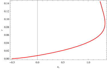
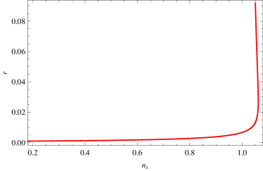
Figure 3: Plot of tensor-scalar ratio $r$ versus scalar spectral index $n_{s}$ for GCCG model in weak dissipative regime (left panel) and strong dissipative regime (right panel)

The plots of $r$ versus $n_{s}$ for GCCG models in weak and strong regime are shown in Figure 3. The constant parameters are $\lambda=1$, $\omega=-0.5$, $M_{p}=1$, $\lambda_{*}=10^{-2}$, $A=10^{-5}$, $b=30$. In weak regime (left panel), the tensor scalar ratio is confined to $r<0.12$ when spectral index is $n_{s}<1$. In strong regime, we get $r<0.08$ for $b=80,~{}0.2<n_{s}<1$. These values shows that GCCG model is compatible with data provided by WMAP$9$ and Planck [32, 33].

4 Conclusions

Warm inflation presents a compelling solution for the main problem of the inflationary theory that how this inflationary period will come to an end. In this type of models, radiations are produced during inflation, and a dissipative coefficient is introduced. This is the reason, we have investigated the warm inflationary scenario inspired with quartic form of potential $V=\frac{\lambda_{*}\phi^{4}}{4}$ and well-known form of dissipative coefficient $\Gamma\propto T$. In order to find the consistency of the results, we have assumed various well-known chaplygin gas models such as GCG, MCG and GCCG. Also, we have considered that this universe is filled with radiation and standard scalar field and accordingly Friedmann equations are modified. Under slow roll approximation, we have investigated inflationary parameters such as number of e-folds, scalar spectrum, scaler spectral index, and tensor to scalar ratio both in weak and strong dissipative regimes.

To analyze our results, we have plotted the graphs between tensor to scalar ratio $r$ and scalar spectral index $n_{s}$ for each model in weak (where $\Gamma\ll 3H$) and strong (where $\Gamma\gg 3H$) dissipative regimes. For GCG model, it is found that in weak dissipative regime with $0.4<n_{s}<1$, we have $r<0.006$, and in strong dissipative regime, $r=0.05$ at $n_{s}=0.96$ (referred as Figure 1). In MCG model, spectral index lies between $0.6<n_{s}<1$, the range of tensor scalar ratio is $r<0.045$ in weak regime. However, in strong regime, we have obtained the range $r<0.15$ for $0.7<n_{s}<1$. In GCCG model, for the weak regime when spectral index is $n_{s}<1$, the tensor scalar ratio is confined to $r<0.12$. But, in strong regime for $b=80$, $0.2<n_{s}<1$, we get $r<0.08$.

In addition, WMAP$9$ provides the value of tensor scalar ratio $r<0.13$ and spectral index is measured to be $n_{s}=0.972\pm 0.013$, according to Planck data $r<0.11$ and $n_{s}=0.968\pm 0.006$. We have concluded with good remark that the obtain range/values of $r$ corresponding to well-settled $n_{s}$ are well supported to WMAP9 [32] and Planck data [33] in all models of CG models.

References

- [1] Starobinsky, A.A.: Phys. Lett. B 91(1980); Guth, A.: Phys. Rev. D 23(1981)347.
- [2] Gold, B. et al.: Astrophy. J. Suppl. 192(2011)15.
- [3] Berera, A.: Phys. Rev. Lett. 75(1995)3218.
- [4] Berera, A.: Phys. Rev. D 55(1995)3346.
- [5] Hall, L.M.H., Moss, I.G., Berera, A.: Phys. Rev. D 69(2004)083525.
- [6] Berera, A.: Phys. Rev. D 54(1996)2519.
- [7] Moss, I.G.: Phys. Lett. B 154(1985)120.
- [8] Berera, A., Fang, L.Z.: Phys. Rev. Lett. 74(1995)1912.
- [9] Berera, A.: Nucl. Phys. B 585(2000)666.
- [10] Pich, A.: arXiv:0705.4264[hep-ph].
- [11] Monerat, G.A. et al.: Phys. Rev. D 76(2007)02017.
- [12] Antonella cid, M., Del Campo, S., Herrera, R.: JCAP 0710(2007)005.
- [13] Del Campo, S., Herrera, R.: Phys. Lett. B 660(2008)282.
- [14] Setare, M.R., Kamali, V.: JCAP 08(2012).
- [15] Antonella cid, M., Del Campo, S., Herrera, R.: JCAP 0710(2007)005.
- [16] Bastero-Gil, M., Berera, A., Ramos, R.O., Rosa, J.G.: JCAP 1301(2013)016.
- [17] Setare, M.R., Kamali, V.: Phys. Rev. D 87(2013)083524.
- [18] Herrera, R., Olivares, M., Videla, N.: Eur. Phys. J. C 73(2013)2295.
- [19] Herrera, R., Olivares, M., Videla, N.: Phys. Rev. D 88(2013)063535.
- [20] Herrera, R., Olivares, M., Videla, N.: Mod. Phys. D 23(2014)1450080.
- [21] Bastero-Gil, M., Berera, A., Ramos, R.O., Rosa, J.G.: JCAP 1410(2014)10053.
- [22] Sharif, M., Saleem, R.: Eur. Phys. J. C 74(2014).
- [23] Setare, M.R., Kamali, V.: Class. Quantum Grav. 32(2015)235005.
- [24] Setare, M.R., Kamali, V.: Int. J. Theor. Phys. 55(2016)103.
- [25] Panotopoulos, G., Videla, N.: Eur. Phys. J. C 75 (2015)
- [26] Zhang, Y.: JCAP 0903(2009)023.
- [27] Bastero-Gil, M., Berera, A., Ramos, R.O.: JCAP 1107(2011)030.
- [28] Berera, A., Gleiser, M., Ramos, R.O.: Phys. Rev. D 58(1998)123508.
- [29] Yokoyama, J., Linde, A.: Phys. Rev. D 60(1999)083500.
- [30] Bento, M.S., Bertolami, O., Sen, A.: Phys. Rev. D 66(2002)043507.
- [31] Kamenshchik, A., Moschell, U. and Pasquier, V.: Phys. Lett. B 511(2001)265.
- [32] Ade, P.A.R., et al.: Astron. Astro phys. A 16(2014)571.
- [33] Hinshaw, G., et al.: Astrophys. J. Suppl. 208(2013)19.
- [34] Benaoum, H.B., Debnath, U., Banerjee, A. and Chakraborty, S.: Class. Quantum Grav. 21(2011)5609.
- [35] Gonzalez-Diaz, P.F.: Phys. Rev. D 68(2003)021303.