750 GeV diphoton resonance and electric dipole moments

Abstract

We examine the implication of the recently observed 750 GeV diphoton excess for the electric dipole moments of the neutron and electron. If the excess is due to a spin zero resonance which couples to photons and gluons through the loops of massive vector-like fermions, the resulting neutron electric dipole moment can be comparable to the present experimental bound if the CP-violating angle $\alpha$ in the underlying new physics is of ${\cal O}(10^{-1})$. An electron EDM comparable to the present bound can be achieved through a mixing between the 750 GeV resonance and the Standard Model Higgs boson, if the mixing angle itself for an approximately pseudoscalar resonance, or the mixing angle times the CP-violating angle $\alpha$ for an approximately scalar resonance, is of ${\cal O}(10^{-3})$. For the case that the 750 GeV resonance corresponds to a composite pseudo-Nambu-Goldstone boson formed by a QCD-like hypercolor dynamics confining at $\Lambda_{\rm HC}$, the resulting neutron EDM can be estimated with $\alpha\sim(750\,{\rm GeV}/\Lambda_{\rm HC})^{2}\theta_{\rm HC}$, where $\theta_{\rm HC}$ is the hypercolor vacuum angle.

I Introduction

Recently the ATLAS and CMS collaborations reported an excess of diphoton events at the invariant mass $m_{\gamma\gamma}\simeq 750$ GeV with the local significance 3.6 $\sigma$ and 2.6 $\sigma$, respectively ATLAS ; CMS . The analysis was updated later, yielding an increased local significance, 3.9 $\sigma$ and 3.4 $\sigma$, respectively ATLAS1 ; CMS1 . If the signal persists, this will be an unforeseen discovery of new physics beyond the Standard Model (SM). So one can ask now what would be the possible phenomenology other than the diphoton excess, which may result from the new physics to explain the 750 GeV diphoton excess.

With the presently available data, one simple scenario to explain the diphoton excess is a SM-singlet spin zero resonance $S$ which couples to massive vector-like fermions carrying non-zero SM gauge charges Franceschini:2015kwy . In this scenario, the 750 GeV resonance interacts with the SM sector dominantly through the SM gauge fields and possibly also through the Higgs boson. In such case, if the new physics sector involves a CP-violating interaction, the electric dipole moment (EDM) of the neutron or electron may provide the most sensitive probe of new physics in the low energy limit.

More explicitly, after integrating out the massive vector-like fermions, the effective lagrangian may include

$$\begin{split}\frac{\kappa_{s}}{2}SF^{a\mu\nu}F^{a}_{\mu\nu}+\frac{\kappa_{p}}{2}SF^{a\mu\nu}\tilde{F}^{a}_{\mu\nu}+\frac{d_{W}}{3}f_{abc}F^{a}_{\mu\rho}F_{\nu}^{b\,\,\rho}\widetilde{F}^{c\mu\nu}+...,\end{split}$$ (1)

where $F^{a}_{\mu\nu}$ denotes the SM gauge field strength and $\tilde{F}^{a}_{\mu\nu}=\frac{1}{2}\epsilon_{\mu\nu\rho\sigma}F^{a\mu\nu}$ is its dual. In view of that the SM weak interactions break CP explicitly through the complex Yukawa couplings, it is quite plausible that the underlying dynamics of $S$ generically breaks CP, which would result in nonzero value of the effective couplings $\kappa_{s}\kappa_{p}/\sqrt{\kappa_{s}^{2}+\kappa_{p}^{2}}$ and $d_{W}$. As is well known, in the presence of those CP violating couplings, a nonzero neutron or electron EDM can be induced through the loops involving the SM gauge fields Weinberg:1989dx ; Barr:1990vd ; Marciano:1986eh ; Boudjema:1990dv .

In this paper, we examine the neutron and electron EDM in models for the 750 GeV resonance, in which the effective interactions (1) are generated by the loops of massive vector-like fermions. We find that for the parameter region to give the diphoton cross section $\sigma(pp\rightarrow\gamma\gamma)=1\sim 10$ fb, the neutron EDM can be comparable to the present experimental bound, e.g. $d_{n}\sim{\rm a\,\,few}\times 10^{-26}\,\,{\rm e\cdot cm}$, if the CP-violating angle $\alpha$ in the underlying dynamics is of ${\cal O}(10^{-1})$, where $\sin 2\alpha\sim\kappa_{s}\kappa_{p}/\sqrt{\kappa^{2}_{s}+\kappa_{p}^{2}}$ in terms of the effective couplings in (1). An electron EDM near the present bound can be obtained also through a mixing between $S$ and the SM Higgs boson $H$. We find that again for the parameter region of $\sigma(pp\rightarrow\gamma\gamma)=1\sim 10$ fb, the electron EDM is given by $d_{e}\sim 6\times 10^{-26}\sin\xi_{SH}\sin\alpha\,\,{\rm e\cdot cm}$, where $\xi_{SH}$ is the $S-H$ mixing angle. Our result on the neutron EDM can be applied also to the models in which $S$ corresponds to a composite pseudo-Nambu-Goldstone boson formed by a QCD-like hypercolor dyanmics which is confining at $\Lambda_{\rm HC}$ Harigaya:2015ezk ; Nakai:2015ptz ; Redi:2016kip . In this case, the CP-violating order parameter $\alpha$ can be identified as $\alpha\sim\theta_{\rm HC}m_{S}^{2}/\Lambda^{2}_{\rm HC}$, where $\theta_{\rm HC}$ denotes the vacuum angle of the underlying QCD-like hypercolor dynamics.

The organization of this paper is as follows. In section II, we introduce a simple model for the 750 GeV resonance involving CP violating interactions, and summarize the diphoton signal rate given by the model. In section III, we examine the neutron and electron EDM in the model of section II, and discuss the connection between the resulting EDMs and the diphoton signal rate. Although we are focusing on a specific model, our results can be used for an estimation of EDMs in more generic models for the 750 GeV resonance. In section IV, we apply our result to the case that $S$ is a composite pseudo-Nambu-Goldstone boson formed by a QCD-like hypercolor dynamics. Section V is the conclusion.

II A model for diphoton excess with CP violation

The 750 GeV diphoton excess can be explained most straightforwardly by introducing a SM-singlet spin zero resonance $S$ which couples to massive vector-like fermions to generate the effective interactions (1) Franceschini:2015kwy . To be specific, here we consider a simple model involving $N_{F}$ Dirac fermions $\Psi=(\Psi_{1},\Psi_{2},...,\Psi_{N_{F}})$ carrying a common charge under the SM gauge group $SU(3)_{c}\times SU(2)_{L}\times U(1)_{Y}$. Then the most general renormalizable interactions of $S$ and $\Psi$ include

$${\cal L}=\bar{\Psi}i\not{D}\Psi-\bar{\Psi}\left(M+Y_{s}S+iY_{p}S\gamma^{5}\right)\Psi-\frac{1}{2}m_{S}^{2}S^{2}-A_{SH}S|H|^{2}+...,$$ (2)

where the mass matrix $M$ can be chosen to be real and diagonal, while $Y_{s,p}$ are hermitian Yukawa coupling matrices. Here $H$ is the SM Higgs doublet, and we have chosen the field basis for which $S$ has a vanishing vacuum expectation value in the limit to ignore its mixing with $H$. For simplicity, in the following we assume that all fermion masses and the Yukawa couplings are approximately flavor-universal, so they can be parametrized as

$$M\,\approx\,m_{\Psi}\,{\bf 1}_{N_{F}\times N_{F}},\quad Y_{s}\approx y_{S}\cos\alpha\,{\bf 1}_{N_{F}\times N_{F}},\quad Y_{p}\approx y_{S}\sin\alpha\,{\bf 1}_{N_{F}\times N_{F}},$$ (3)

where ${\bf 1}_{N_{F}\times N_{F}}$ denotes the $N_{F}\times N_{F}$ unit matrix. Note that in this parametrization $\sin 2\alpha$ corresponds to the order parameter for CP violation. In the following, we will often use $\alpha$ (or $\sin\alpha$) as a CP violating order parameter, although it should be $\alpha-\pi/2$ (or $\cos\alpha$) for an approximately pseudoscalar $S$.

Under the above assumption on the model parameters, one can compute the 1PI amplitudes for the production and decay of $S$ at the LHC, yielding Franceschini:2015kwy

$$\begin{split}{\cal L}_{\rm 1PI}&=\frac{g_{3}^{2}}{16\pi^{2}m_{S}}S\left(c^{(s)}_{3}G^{a}_{\mu\nu}G^{a\mu\nu}+c^{(p)}_{3}G^{a}_{\mu\nu}\widetilde{G}^{a\mu\nu}\right)\\ &+\frac{g_{2}^{2}}{16\pi^{2}m_{S}}S\left(c^{(s)}_{2}W^{a}_{\mu\nu}W^{a\mu\nu}+c^{(p)}_{2}W^{a}_{\mu\nu}\widetilde{W}^{a\mu\nu}\right)\\ &+\frac{g_{1}^{2}}{16\pi^{2}m_{S}}S\left(c^{(s)}_{1}B_{\mu\nu}B^{\mu\nu}+c^{(p)}_{1}B_{\mu\nu}\widetilde{B}^{\mu\nu}\right),\end{split}$$ (4)

where

$$\begin{split}c_{i}^{(s)}&=N_{F}y_{S}\cos\alpha\,{\rm Tr}(T_{i}^{2}(\Psi))\frac{m_{S}}{m_{\Psi}}\frac{A_{1/2}(\tau_{\Psi})}{2},\\ c_{i}^{(p)}&=-N_{F}y_{S}\sin\alpha\,{\rm Tr}(T_{i}^{2}(\Psi))\frac{m_{S}}{m_{\Psi}}\frac{f(\tau_{\Psi})}{\tau_{\Psi}},\end{split}$$ (5)

with $i=1,\,2,\,3$ denoting the SM gauge groups $U(1)_{Y},\,SU(2)_{L},\,SU(3)_{c}$, respectively, and $\tau_{\Psi}\equiv m_{S}^{2}/4m_{\Psi}^{2}$. The loop functions $A_{1/2}(\tau)$ and $f(\tau)$ are given by

$$A_{1/2}(\tau) = 2\big{[}\tau+(\tau-1)f(\tau)]/\tau^{2},$$

$$f(\tau) = -\frac{1}{2}\int_{0}^{1}dx\frac{1}{x}\ln[1-4x(1-x)\tau]$$ (8)

$$= \left\{\begin{array}[]{ll}(\arcsin\sqrt{\tau})^{2},&\tau\leq 1\\ -\frac{1}{4}\left[\ln\left(\frac{1+\sqrt{1-\tau^{-1}}}{1-\sqrt{1-\tau^{-1}}}\right)-i\pi\right]^{2},&\tau>1.\end{array}\right.$$

Note that with a nonzero value of the CP violating angle $\alpha$, the 750 GeV resonance $S$ couples to both $F^{a}_{\mu\nu}F^{a\mu\nu}$ and $F^{a}_{\mu\nu}\widetilde{F}^{a\mu\nu}$. These two couplings turn out to incoherently contribute to the decay rate of $S$, so that the relevant decay rates are given by

$$\Gamma_{\gamma\gamma} = \frac{1}{4\pi}\left(\frac{e^{2}}{16\pi^{2}}\right)^{2}m_{S}\left(\left|c_{\gamma}^{(s)}\right|^{2}+\left|c_{\gamma}^{(p)}\right|^{2}\right),$$ (9)

$$\Gamma_{gg} = \frac{8}{4\pi}\left(\frac{g_{3}^{2}}{16\pi^{2}}\right)^{2}m_{S}\left(\left|c_{g}^{(s)}\right|^{2}+\left|c_{g}^{(p)}\right|^{2}\right),$$ (10)

in the rest frame of $S$. The diphoton signal cross section at the LHC can be estimated using the narrow width approximation Franceschini:2015kwy , yielding

$$\sigma(pp\rightarrow S\rightarrow\gamma\gamma)=C_{gg}\frac{1}{s}\frac{m_{S}}{\Gamma_{S}}\frac{\Gamma_{\gamma\gamma}}{m_{S}}\frac{\Gamma_{gg}}{m_{S}},$$ (11)

where the coefficient $C_{gg}=2137$ at $\sqrt{s}=13$ TeV, and $\Gamma_{S}$ denotes the total decay width of $S$. Manipulating this, the decay rate should satisfy the following relation,

$$\begin{split}\frac{\Gamma_{\gamma\gamma}}{m_{S}}\frac{\Gamma_{gg}}{m_{S}}=2.17\times 10^{-9}\left(\frac{\Gamma_{S}}{1\,{\rm GeV}}\right)\left(\frac{\sigma_{\rm signal}}{8\,{\rm fb}}\right),\end{split}$$ (12)

for the signal cross section $\sigma=1\sim 10$ fb. Here we normalize the total decay rate of $S$ by $\Gamma_{S}=1$ GeV, since it is a typical value when there is an appreciable mixing between the singlet scalar $S$ and the SM Higgs doublet Falkowski:2015swt .

Plugging (5) and (9, 10) into (12), we obtain a relation which is useful for an estimation of the electric dipole moments over the diphoton signal region:

$$\begin{split}\frac{m_{\Psi}}{y_{S}}=96\,{\rm GeV}\times Q_{\Psi}N_{F}\left(\frac{2}{3}{\rm Tr}(T_{3}^{2}(\Psi)){\rm Tr}({\bf 1}(\Psi))\right)^{1/2}\left(\frac{1\,\rm GeV}{\Gamma_{S}}\right)^{1/4}\left(\frac{8\,\rm fb}{\sigma_{\rm signal}}\right)^{1/4}R_{\Psi},\end{split}$$ (13)

where

$$R_{\Psi}(\alpha,\tau_{\Psi}=m_{S}^{2}/4m^{2}_{\Psi})=\left(\frac{c_{\alpha}^{2}(A_{1/2}(\tau_{\Psi})/2)^{2}+s_{\alpha}^{2}(f(\tau_{\Psi})/\tau_{\Psi})^{2}}{c_{0.1}^{2}(A_{1/2}(1/4)/2)^{2}+s_{0.1}^{2}(4f(1/4))^{2}}\right)^{1/2}=\,{\cal O}(1).$$

Here $Q_{\Psi}$ and $T_{3}(\Psi)$ denote the electromagnetic and color charge of $\Psi$, respectively, ${\rm Tr}({\bf 1}(\Psi))$ is the dimension of the gauge group representation of $\Psi$, and $s_{\alpha}=\sin\alpha$ and $c_{\alpha}=\cos\alpha$. Note that $R_{\Psi}$ represents the dependence on $\tau_{\Psi}=m_{S}^{2}/4m^{2}_{\Psi}$ and $\alpha$, which is normalized to the value at $\tau_{\Psi}=1/4$ and $\alpha=0.1$. As $R_{\Psi}$ has a mild dependence on $\tau_{\Psi}$ and $\alpha$, the range of the parameter ratio $m_{\Psi}/y_{S}$ which would explain the diphoton excess can be easily read off from the above relation.

To see the origin of the CP violating angle $\alpha$, one may consider a UV completion of the model (2). In regard to this, an attractive possibility is that the model is embedded at some higher scales into a supersymmetric model including a singlet superfield $\phi$ and $N_{F}$ flavors of vector-like charged matter superfields $\psi+\psi^{c}$ Hall:2015xds ; Nilles:2016bjl . The most general renormalizable superpotential of $\phi$ and $\psi+\psi^{c}$ is given by

$$W=(M+Y\phi)\psi\psi^{c}+\frac{1}{2}\mu_{\phi}\phi^{2}+\frac{1}{3}\kappa\phi^{3},$$ (14)

where without loss of generality $M$ can be chosen to be real and diagonal, ${\rm det}(Y)$ to be real, and $\phi$ to have a vanishing vacuum value in the limit to ignore the mixing with the Higgs doublets. Again, for simplicity let us assume that the mass matrix $M$ and the Yukawa coupling matrix $Y$ are approximately flavor-universal, and therefore

$$M\approx m_{\Psi}{\bf 1}_{N_{F}\times N_{F}},\quad Y\approx y_{S}{\bf 1}_{N_{F}\times N_{F}}.$$ (15)

Including the soft supersymmetry (SUSY) breaking terms, the scalar mass term of $\phi$ is given by

$$\left(|\mu_{\phi}|^{2}+m_{\phi}^{2}\right)|\phi|^{2}+\frac{1}{2}\left(B_{\phi}\mu_{\phi}\phi^{2}+{\rm h.c}\right),$$ (16)

where $m_{\phi}$ is a SUSY breaking soft scalar mass, while $B$ is a holomorphic bilinear soft parameter. Note that in our prescription, both $\mu_{\phi}$ and $B_{\phi}$ are complex in general.

Without relying on any fine tuning other than the minimal one to keep the SM Higgs to be light, one can arrange the SUSY model parameters to identify the lighter mass eigenstate of $\phi$ as the 750 GeV resonance $S$, and the fermion components of $\psi+\psi^{c}$ as the Dirac fermion $\Psi$ to generate the effective interactions (4), while keeping all other SUSY particles heavy enough to be in multi-TeV scales. Then our model (2) arises as a low energy effective theory at scales around TeV from the SUSY model (14), with the matching condition

$$\frac{1}{\sqrt{2}}S={\rm Re}(\phi)\cos\alpha+{\rm Im}(\phi)\sin\alpha,$$

where

$$\tan 2\alpha=\frac{{\rm Im}(B_{\phi}\mu_{\phi})}{{\rm Re}(B_{\phi}\mu_{\phi})}.$$ (17)

Another possibility, which is completely different but equally interesting, would be that $S$ corresponds to a pseudo-Nambu-Goldstone boson formed by a QCD-like hypercolor dynamics which confines at scales near TeV. As we will see in section IV, the CP violating order parameter $\alpha$ in such models can be identified as

$$\sin 2\alpha\sim\frac{m_{S}^{2}}{\Lambda_{\rm HC}^{2}}\sin\theta_{\rm HC},$$ (18)

where $\Lambda_{\rm HC}$ is the scale of spontaneous chiral symmetry breaking by the hypercolor dynamics and $\theta_{\rm HC}$ is the hypercolor vacuum angle.

III Electric Dipole Moments

In this section, we estimate the electric dipole moments (EDMs) induced by the 750 GeV sector in terms of the model introduced in the previous section. At energy scales below $m_{\Psi}$ and $m_{S}$, the heavy fermions $\Psi$ and the singlet scalar $S$ can be integrated out, while leaving their footprints in the effective interactions among the SM gauge bosons and Higgs boson. Then those effective interactions eventually generate the nucleon and electron EDMs in the low energy limit through the loops involving the exchange of the SM gauge bosons and/or the Higgs boson. In this process, one needs to take into account the renormalization group (RG) running, particularly those due to the QCD interactions, from the initial threshold scale $m_{\Psi}\sim m_{S}$ down to the hadronic scale $\Lambda_{\rm QCD}$, as well as the intermediate threshold corrections from integrating out the massive SM particles.

To simplify the calculation, we will ignore the RG running effects due to the QCD interactions over the scales from $m_{\Psi}$ to the SM Higgs boson mass $m_{H}=125$ GeV. In this approximation, the Wilsonian effective interactions at scales just below $m_{H}$ can be determined by the leading order Feynman diagrams involving $\Psi,S$ and the SM Higgs boson. We then take into account the subsequent RG running due to the QCD interactions from $m_{H}$ to $\Lambda_{\rm QCD}$, while ignoring the threshold corrections due to the SM heavy quarks, to derive the low energy effective lagrangian at scales just above $\Lambda_{\rm QCD}$.

III.1 Neutron EDM

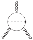
Figure 1: The Weinberg’s three gluon interaction generated as a two-loop threshold correction. Here the small dark square represents the $\gamma_{5}$-coupling of $S$ to the vector-like fermion $\Psi$.

The leading contribution to the neutron EDM turns out to come from the Weinberg’s three gluon operator Weinberg:1989dx generated by the diagram in Fig. 1. In the presence of a mixing between the singlet scalar $S$ and the SM Higgs boson $H$, the EDM and chromo EDM (CEDM) of light quarks are induced by the Barr-Zee diagrams Barr:1990vd in Fig. 2, which may provide a potentially important contribution to the neutron EDM.

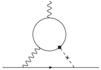
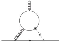
Figure 2: The Barr-Zee diagrams for the EDM and chromo EDM (CEDM) of light fermions. The small cross denotes the $S-H$ mixing.

To be concrete, let us take a simple model having $N_{F}$ vector-like Dirac fermions $\Psi$ transforming under $SU(3)_{c}\times SU(2)_{L}\times U(1)_{Y}$ as

$$\begin{split}\Psi=(3,1)_{Y_{\Psi}},\end{split}$$ (19)

where $Y_{\Psi}$ denotes the $U(1)_{Y}$ hypercharge of $\Psi$. As mentioned above, we take an approximation to ignore the RG running due to the QCD interactions between $m_{\Psi}$ and $m_{H}=125$ GeV. Then at scales just below $m_{H}$, the relevant Wilsonian effective interactions are determined to be Weinberg:1989dx ; Abe:2013qla ; Dicus:1989va ; Jung:2013hka ; Dekens:2014jka ,

$${\cal L_{\rm eff}}(m_{H}) = -\frac{d_{W}(m_{H})}{6}f_{abc}\epsilon^{\mu\nu\rho\sigma}G^{a}_{\rho\sigma}G^{b}_{\mu\lambda}G^{c\,\,\lambda}_{\nu}$$ (20)

$$-\frac{i}{2}\sum_{q}\Big{[}d_{q}(m_{H})e\bar{q}\sigma^{\mu\nu}\gamma_{5}qF_{\mu\nu}+\tilde{d}_{q}(m_{H})g_{3}\bar{q}\sigma^{\mu\nu}\gamma_{5}T_{3}^{a}qG^{a\mu\nu}\Big{]}+...,$$

with

$$d_{q}(m_{H}) = 4N_{F}\frac{e^{2}}{(4\pi)^{4}}\frac{m_{q}}{v}\left(6Y_{\Psi}^{2}\frac{y_{S}}{m_{\Psi}}s_{\alpha}s_{\xi}c_{\xi}\right)\left[Q_{q}+\left(t_{w}^{2}Q_{q}-\frac{T^{3}_{q_{L}}}{2c_{w}^{2}}\right)\right]\left[g\left(\frac{m_{\Psi}^{2}}{m_{H}^{2}}\right)-g\left(\frac{m_{\Psi}^{2}}{m_{S}^{2}}\right)\right],$$

$$\tilde{d}_{q}(m_{H}) = 4N_{F}\frac{g_{3}^{2}}{(4\pi)^{4}}\frac{m_{q}}{v}\left(\frac{y_{S}}{m_{\Psi}}s_{\alpha}s_{\xi}c_{\xi}\right)\left[g\left(\frac{m_{\Psi}^{2}}{m_{H}^{2}}\right)-g\left(\frac{m_{\Psi}^{2}}{m_{S}^{2}}\right)\right],$$

$$d_{W}(m_{H}) = -N_{F}\frac{g_{3}^{3}}{(4\pi)^{4}}\frac{y_{S}^{2}}{m_{\Psi}^{2}}c_{\alpha}s_{\alpha}\left[s_{\xi}^{2}h\left(\frac{m_{\Psi}^{2}}{m_{H}^{2}}\right)+c_{\xi}^{2}h\left(\frac{m_{\Psi}^{2}}{m_{S}^{2}}\right)\right],$$ (21)

where $q=u,d,s$ stands for the light quark species, $s_{\alpha}=\sin\alpha$, $s_{\xi}=\sin\xi_{SH}$ for the $S-H$ mixing angle $\xi_{SH}$, $v=246$ GeV is the SM Higgs vacuum value, $c_{w}=\cos\theta_{w}$, $t_{w}=\tan\theta_{w}$ for the weak mixing angle $\theta_{w}$, and the loop functions $g$ and $h$ are given by

$$g(z) \equiv \frac{z}{2}\int^{1}_{0}dx\frac{1}{x(1-x)-z}\ln\frac{x(1-x)}{z},$$

$$h(z) \equiv z^{2}\int^{1}_{0}dx\int^{1}_{0}dy\frac{x^{3}y^{3}(1-x)}{[zx(1-xy)+(1-x)(1-y)]^{2}}.$$ (22)

Let us recall that the parameter ratio $m_{\Psi}/y_{S}$ has a specific connection with the diphoton cross section $\sigma(pp\rightarrow\gamma\gamma)$, which is given by (13). This allows us to estimate the expected size of the EDMs in terms of a few model parameters such as $\alpha$ and $\xi_{SH}$.

In order to estimate the resulting neutron EDM, we should bring the effective interactions (20) down to the QCD scale through the RG evolution. For this, it is convenient to redefine the coefficients as

$$C_{1}(\mu)=\frac{d_{q}(\mu)}{m_{q}Q_{q}},\quad{C}_{2}(\mu)=\frac{\tilde{d}_{q}(\mu)}{m_{q}},\quad C_{3}(\mu)=\frac{d_{W}(\mu)}{g_{3}},$$ (23)

which are satisfying the RG equation Degrassi:2005zd ; Hisano:2012cc :

$$\mu\frac{\partial{\bf C}}{\partial\mu}=\frac{g_{3}^{2}}{16\pi^{2}}\gamma\,{\bf C},$$ (24)

with the anomalous dimension matrix

$$\gamma\equiv\left(\begin{array}[]{ccc}\gamma_{e}&\gamma_{eq}&0\\ 0&\gamma_{q}&\gamma_{Gq}\\ 0&0&\gamma_{G}\end{array}\right)=\left(\begin{array}[]{ccc}8C_{F}&8C_{F}&0\\ 0&16C_{F}-4N_{c}&2N_{c}\\ 0&0&N_{c}+2n_{f}+\beta_{0}\end{array}\right),$$ (31)

where ${\bf C}=(C_{1},{C}_{2},C_{3})^{T}$, $N_{c}=3$ is the number of color, $C_{F}=4/3$ is a quadratic Casimir, $n_{f}$ is the number of active light quarks, and $\beta_{0}=(33-2n_{f})/3$ is the one-loop beta function coefficient. Solving this RG equations, one finds Degrassi:2005zd

$$C_{1}(\mu) = \eta^{\kappa_{e}}C_{1}(m_{H})+\frac{\gamma_{qe}}{\gamma_{e}-\gamma_{q}}(\eta^{\kappa_{e}}-\eta^{\kappa_{q}})C_{2}(m_{H})$$

$$+ \left[\frac{\gamma_{Gq}\gamma_{qe}\eta^{\kappa_{e}}}{(\gamma_{q}-\gamma_{e})(\gamma_{G}-\gamma_{e})}+\frac{\gamma_{Gq}\gamma_{qe}\eta^{\kappa_{q}}}{(\gamma_{e}-\gamma_{q})(\gamma_{G}-\gamma_{q})}+\frac{\gamma_{Gq}\gamma_{qe}\eta^{\kappa_{G}}}{(\gamma_{e}-\gamma_{G})(\gamma_{q}-\gamma_{G})}\right]C_{3}(m_{H}),$$

$$C_{2}(\mu) = \eta^{\kappa_{q}}C_{2}(m_{H})+\frac{\gamma_{Gq}}{\gamma_{q}-\gamma_{G}}\left[\eta^{\kappa_{q}}-\eta^{\kappa_{G}}\right]C_{3}(m_{H}),$$

$$C_{3}(\mu) = \eta^{\kappa_{G}}C_{3}(m_{H}),$$ (32)

where $\eta\equiv g_{3}^{2}(m_{H})/g_{3}^{2}(\mu)$ and $\kappa_{x}=\gamma_{x}/(2\beta_{0})$. The analytic expressions for $C_{i}(\mu\sim\Lambda_{\rm QCD})$ in terms of $C_{i}(m_{H})$ are complicated except $C_{3}$, however fortunately it turns out that the dominant contribution to the neutron EDM comes from $C_{3}(\mu\sim\Lambda_{\rm QCD})$. From (32), we obtain

$$\begin{split}d_{W}(\mu)=\left(\frac{g_{3}(m_{c})}{g_{3}(\mu)}\right)\left(\frac{g_{3}(m_{b})}{g_{3}(m_{c})}\right)^{\frac{33}{25}}\left(\frac{g_{3}(m_{H})}{g_{3}(m_{b})}\right)^{\frac{39}{23}}d_{W}(m_{H}).\end{split}$$ (33)

It can be shown numerically that $d_{q}(\mu)$ and $\tilde{d}_{q}(\mu)$ also get a similar amount of suppression by the RG evolution compared to the high scale values at $m_{H}$.

Now one can relate the Wilsonian coefficients $d_{W}(\mu),d_{q}(\mu)$ and $\tilde{d}_{q}(\mu)$ at $\mu\sim\Lambda_{\rm QCD}$ to the neutron EDM:

$$-\frac{i}{2}d_{n}\bar{n}\sigma^{\mu\nu}\gamma_{5}nF_{\mu\nu},$$ (34)

which is the most ambiguous step. For this, one can take two approaches, the Naive Dimensional Analysis (NDA) NDA or the QCD sum rule Pospelov:2000bw ; Hisano:2012sc ; Hisano:2015rna , essentially yielding similar results. As for the neutron EDM estimated by the NDA, one finds

$$d_{n}/e={\cal O}(d_{q}(\mu))+{\cal O}(\tilde{d}_{q}(\mu)/\sqrt{6})+{\cal O}(f_{\pi}d_{W}(\mu)),$$ (35)

where the corresponding scale $\mu$ is chosen to be the one with $g_{3}(\mu)\simeq 4\pi/\sqrt{6}$ Weinberg:1989dx . On the other hand, applying the QCD sum rule for the neutron EDM $d^{q}_{n}$ from the (C)EDM of light quarks, one finds a more concrete result Hisano:2015rna :

$$d^{q}_{n}/e\simeq-0.2d_{u}(\mu)+0.78d_{d}(\mu)+0.29\tilde{d}_{u}(\mu)+0.59\tilde{d}_{d}(\mu).$$ (36)

for $\mu\simeq 1$ GeV. As for the neutron EDM $d^{W}_{n}$ from the Weinberg’s three gluon operator in the QCD sum rule approach, one similarly finds Demir:2002gg

$$|d^{W}_{n}/e|=\left(1.0^{+1.0}_{-0.5}\right)\times 20\,{\rm MeV}\times|d_{W}(\mu)|$$ (37)

for $\mu\simeq 1$ GeV. We can now make a comparison between the neutron EDM $d_{n}^{W}$ originating from $d_{W}(\mu)$ and the other part $d_{n}^{q}$ originating from $d_{q}(\mu)$ and $\tilde{d}_{q}(\mu)$. Within the QCD sum rule approach, we find numerically

$$\begin{split}{d_{n}^{q}}/{d_{n}^{W}}\,\simeq\,3\,\sin\xi_{SH}+0.07.\end{split}$$ (38)

This implies that the neutron EDM is dominated by the contribution from the Weinberg’s three gluon operator for the $S-H$ mixing angle $\xi_{SH}\lesssim 0.1$, which might be required to be consistent with the Higgs precision data Falkowski:2015swt ; Cheung:2015cug .

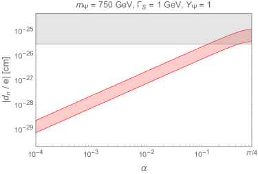
Figure 3: The neutron electric dipole moment as a function of the CP violating angle $\alpha$ for the model parameters to give $\sigma_{\rm signal}=1-10$ fb. For this plot, we choose the total decay width of $S$ as $\Gamma_{S}=1$ GeV, the number of Dirac fermions $\Psi$ as $N_{F}=1$, the mass and $U(1)_{Y}$ hyperchage of $\Psi$ as $m_{\Psi}=750$ GeV and $Y_{\Psi}=1$.

With the above observation, plugging (13), (21) and (33) into (37), we obtain the following expression for the expected neturon EDM over the 750 GeV signal region:

$$\begin{split}d_{n}/e\simeq 3\times 10^{-25}\,{\rm cm}&\times\frac{c_{\alpha}s_{\alpha}}{N_{F}Y_{\Psi}^{2}}\sqrt{\left(\frac{\Gamma_{S}}{1\,\rm GeV}\right)\left(\frac{\sigma_{\rm signal}}{8\,\rm fb}\right)}\times R_{n},\end{split}$$ (39)

where

$$R_{n}=\left(\frac{h(4\tau_{\Psi})}{h(1)}\right)\left[\frac{c_{0.1}^{2}(A_{1/2}(1/4)/2)^{2}+s_{0.1}^{2}(4f(1/4))^{2}}{c_{\alpha}^{2}(A_{1/2}(\tau_{\Psi})/2)^{2}+s_{\alpha}^{2}(f(\tau_{\Psi})/\tau_{\Psi})^{2}}\right]^{1/2}=\,{\cal O}(1).$$

Here $R_{n}$ represents the dependence on the loop functions $A_{1/2},f$ and $h$ defined in (8) and (22), which is normalized to the value at $\tau_{\Psi}=m_{S}^{2}/4m_{\Psi}^{2}=1/4$ and $\alpha=0.1$. With this result, one can easily see that the neutron EDM from the 750 GeV sector saturates the current experimental upper bound $\sim 3\times 10^{-26}\,{\rm e\cdot cm}$ Baker:2006ts for the parameter region with $\sin 2\alpha/N_{F}Y_{\Psi}^{2}\sim 0.1$. In Fig. 3, we depict the resulting neutron EDM as a function of CP violating angle $\alpha$ for the model parameters which give the diphoton cross section $\sigma(pp\rightarrow\gamma\gamma))=1\sim 10$ fb.

III.2 Electron EDM

In the presence of the $S-H$ mixing, a sizable electron EDM can arise from the Barr-Zee diagram in Fig. (2). In case of the model with $N_{F}$ flavors of $\Psi=(3,1)_{Y_{\Psi}}$, we obtain the electron EDM

$$\begin{split}-\frac{ie}{2}d_{e}(\mu)\bar{e}\sigma^{\mu\nu}\gamma_{5}eF_{\mu\nu},\end{split}$$ (40)

with the coefficient Jung:2013hka ; Dekens:2014jka

$$d_{e} = -24N_{F}\frac{e^{2}}{(4\pi)^{4}}\frac{m_{e}}{v}\Big{(}Y_{\Psi}^{2}\frac{y_{S}}{m_{\Psi}}s_{\alpha}s_{\xi}c_{\xi}\Big{)}\Big{(}1+t_{w}^{2}-\frac{1}{4c_{w}^{2}}\Big{)}\left[g\left(\frac{m_{\Psi}^{2}}{m_{H}^{2}}\right)-g\left(\frac{m_{\Psi}^{2}}{m_{S}^{2}}\right)\right],$$ (41)

where the loop function $g(z)$ is given in (22) and the other parameters are defined as same as in (21). Applying the relation (13) for the above result, we find

$$\begin{split}d_{e}=-(6.2&\times 10^{-26}\,{\rm cm})\times s_{\alpha}s_{\xi}c_{\xi}Y_{\Psi}\left(\frac{\Gamma_{S}}{1\,\rm GeV}\right)^{1/4}\left(\frac{\sigma_{\rm signal}}{8\,\rm fb}\right)^{1/4}\times R_{e},\end{split}$$ (42)

where

$$R_{e}=\left(\frac{g(m_{S}^{2}/4\tau_{\Psi}m_{H}^{2})-g(1/4\tau_{\Psi})}{g(m_{S}^{2}/m_{H}^{2})-g(1)}\right)\left(\frac{c_{0.1}^{2}(A_{1/2}(1/4)/2)^{2}+s_{0.1}^{2}(4f(1/4))^{2}}{c_{\alpha}^{2}(A_{1/2}(\tau_{\Psi})/2)^{2}+s_{\alpha}^{2}(f(\tau_{\Psi})/\tau_{\Psi})^{2}}\right)^{1/2}=\,{\cal O}(1)$$

for $\tau_{\Psi}=m_{S}^{2}/4m_{\Psi}^{2}$. The above result shows the electron EDM associated with the $S-H$ mixing can saturate the current experimental upper limit $8.7\times 10^{-29}$ cm Baron:2013eja when $\sin\alpha\sin\xi_{SH}={\cal O}(10^{-3})$. In Fig. (4), we depict the electron EDM over the 750 GeV signal region for the two different values of the $S-H$ mixing angle: $\xi_{SH}=10^{-1}$ and $10^{-2}$.

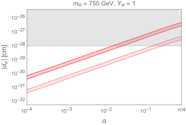
Figure 4: The electron electric dipole moment for the minimal model with $\Psi=(3,1)_{Y_{\Psi}}$, $m_{\Psi}=750$ GeV, $\xi_{SH}=(10^{-1},10^{-2})$, $Y_{\Psi}=1$, and $\sigma_{\rm signal}=1-10$ fb.

If the vector-like fermions $\Psi$ carry a nonzero $SU(2)_{L}$ charge, there can be a nonzero electron EDM even in the limit $\xi_{SH}=0$. For instance, in the model with $N_{F}$ flavors of $\Psi=(3,2)_{Y_{\Psi}}$, a CP-odd three $W$-boson operator of the form

$$\frac{\tilde{d}_{W}}{3}\epsilon_{ijk}W^{i}_{\mu\rho}W_{\nu}^{j\,\,\rho}\widetilde{W}^{k\mu\nu}$$

can be generated by the loops of $\Psi$. Following Marciano:1986eh ; Boudjema:1990dv , we find the resulting electron EDM is given by

$$\begin{split}\Delta d_{e}&\simeq-\frac{N_{F}}{4}\frac{g_{2}^{4}}{(16\pi^{2})^{3}}m_{e}\frac{y_{S}^{2}}{m_{\Psi}^{2}}c_{\alpha}s_{\alpha}\left[s_{\xi}^{2}h\left(\frac{m_{H}^{2}}{m_{\Psi}^{2}}\right)+c_{\xi}^{2}h\left(\frac{m_{S}^{2}}{m_{\Psi}^{2}}\right)\right]\\ &\simeq-(6.5\times 10^{-31}\,{\rm cm})\times\frac{c_{\alpha}s_{\alpha}}{N_{F}Q_{\Psi}^{2}}\sqrt{\left(\frac{\Gamma_{S}}{1\,\rm GeV}\right)\left(\frac{\sigma_{\rm signal}}{8\,\rm fb}\right)}\times\tilde{R}_{e},\end{split}$$ (43)

where

$$\tilde{R}_{e}=\left(\frac{c_{\xi}^{2}h(4\tau_{\Psi})+s_{\xi}^{2}h(m_{H}^{2}/m_{\Psi}^{2})}{c_{0.1}^{2}h(1)+s_{0.1}^{2}h(m_{H}^{2}/m_{S}^{2})}\right)\left(\frac{c_{0.1}^{2}(A_{1/2}(1/4)/2)^{2}+s_{0.1}^{2}(4f(1/4))^{2}}{c_{\alpha}^{2}(A_{1/2}(\tau_{\Psi})/2)^{2}+s_{\alpha}^{2}(f(\tau_{\Psi})/\tau_{\Psi})^{2}}\right)^{1/2}=\,{\cal O}(1).$$

For $\sin 2\alpha\lesssim 0.1$, which might be required to satisfy the bound on the neutron EDM, the resulting electron EDM is about three orders of magnitude smaller than the current bound, therefore too small to be observable in a foreseeable future.

IV Composite pseudo-Nambu-Goldstone resonance

In the previous section, we discussed the neutron and electron EDM in models where the 750 GeV resonance is identified as an elementary spin zero field (at least at scales around TeV) which couples to vector-like fermions to generate the effective couplings to explain the diphoton excess $\sigma(pp\rightarrow\gamma\gamma)\sim 5\,\,{\rm fb}$. On the other hand, it has been pointed out that in most cases this scheme confronts with a strong coupling regime at scales not far above the TeV scale Gu:2015lxj ; Son:2015vfl . In regard to this, an interesting possibility is that $S$ corresponds to a composite pseudo-Nambu-Goldstone (PNG) boson of the spontaneously broken chiral symmetry of a new QCD-like hypercolor dynamics which confines at $\Lambda_{\rm HC}={\cal O}(1)$ TeV Harigaya:2015ezk ; Nakai:2015ptz ; Redi:2016kip . As is well known, such models involve a unique source of CP violation, the hypercolor vacuum angle $\theta_{\rm HC}$, which can yield a nonzero neutron or electron EDM in the low energy limit Harigaya:2015ezk .

To proceed, we consider a specific example, the model discussed in Nakai:2015ptz , involving a hypercolor gauge group $SU(N)_{\rm HC}$ with charged Dirac fermions $(\psi,\chi)$ which transform under $SU(N)_{\rm HC}\times SU(3)_{c}\times SU(2)_{L}\times U(1)_{Y}$ as

$$\psi=(N,3,1)_{Y_{\psi}},\quad\chi=(N,1,1)_{Y_{\chi}},$$ (44)

where $Y_{\psi,\chi}$ denote the $U(1)_{Y}$ hypercharge. At scales above $\Lambda_{HC}$, the lagrangian of the hypercolor color sector is given by

$${\cal L}_{\rm HC} = -\frac{1}{4g_{\rm HC}^{2}}H^{a\mu\nu}H^{a}_{\mu\nu}-\frac{\theta_{\rm HC}}{32\pi^{2}}H^{a\mu\nu}\widetilde{H}^{a}_{\mu\nu}$$ (45)

$$+ \bar{\psi}i\not{D}\psi+\bar{\chi}i\not{D}\chi-\bar{\psi}m_{\psi}\psi-\bar{\chi}m_{\chi}\chi,$$

where $H^{a\mu\nu}$ denotes the $SU(N)_{\rm HC}$ gauge field strength, $\widetilde{H}^{a\mu\nu}$ is its dual, and the fermion masses $m_{\psi,\chi}$ are chosen to be real and $\gamma_{5}$-free. For a discussion of the low energy consequence of the CP-violating vacuum angle $\theta_{\rm HC}$, it is convenient to make a chiral rotation of fermion fields to rotate away $\theta_{\rm HC}$ into the phase of the fermion mass matrix, which results in

$$M=M_{\theta}\equiv\mbox{diag}\left(m_{\psi}e^{ix_{\psi}\theta_{\rm HC}},m_{\psi}e^{ix_{\psi}\theta_{\rm HC}},m_{\psi}e^{ix_{\psi}\theta_{\rm HC}},m_{\chi}e^{ix_{\chi}\theta_{\rm HC}}\right),$$ (46)

where

$$3x_{\psi}+x_{\chi}=1.$$

For $m_{\psi,\chi}\ll\Lambda_{\rm HC}$, the model is invariant under an approximate chiral symmetry $SU(4)_{L}\times SU(4)_{R}$ which is spontaneously broken down to the diagonal $SU(4)_{V}$ by the fermion bilinear condensates:

$$|\langle\bar{\psi}_{L}\psi_{R}\rangle|\,\simeq\,|\langle\bar{\chi}_{L}\chi_{R}\rangle|\,\simeq\,\frac{N}{16\pi^{2}}\Lambda_{\rm HC}^{3}.$$ (47)

The corresponding pseudo-Nambu-Goldstone (PNG) boson can be described by an $SU(4)$-valued field $U=\exp(2i\Phi/f)$ whose low energy dynamics is governed by

$${\cal L}_{\rm eff}=\frac{1}{4}f^{2}\mbox{tr}\left(D_{\mu}UD^{\mu}U^{\dagger}\right)+\mu^{3}\mbox{tr}\left(M_{\theta}U^{\dagger}+\mbox{h.c}\right)+{\cal L}_{\rm WZW}+{\cal L}_{\rm CPV}...,$$ (48)

where the naive dimensional analysis suggests

$$f^{2}\,\simeq\frac{N}{16\pi^{2}}\Lambda_{H}^{2},\quad\mu^{3}\simeq\frac{N}{16\pi^{2}}\Lambda_{H}^{3},$$ (49)

and ${\cal L}_{\rm WZW}$ and ${\cal L}_{\rm CPV}$ denote the Wess-Zumino-Witten term and the additional CP-violating terms, respectively. For a discussion of CP violation due to $\theta_{\rm HC}\neq 0$, it is convenient to choose the fermion mass matrix $M_{\theta}$ as

$$-\frac{i}{2}\left(M_{\theta}-M_{\theta}^{\dagger}\right)=m_{\theta}{\bf 1}_{4\times 4},$$ (50)

for which the PNG boson has a vanishing vacuum expectation value. Then the CP violation due to $\theta_{\rm HC}\neq 0$ is parametrized simply by

$$m_{\theta}\equiv m_{\psi}\sin\left(x_{\psi}{\theta}_{\rm HC}\right)=m_{\chi}\sin\left(x_{\chi}{\theta}_{\rm HC}\right)\quad\left(3x_{\psi}+x_{\chi}=1\right),$$ (51)

which manifestly shows that CP is restored if $\theta_{\rm HC}$ or any of $m_{\psi,\chi}$ is vanishing. In the limit $|\theta_{\rm HC}|\ll 1$, this order parameter for CP violation has a simple expression:

$$m_{\theta}\,\simeq\,\frac{\theta_{\rm HC}}{\mbox{tr}\left(M^{-1}_{\bar{\theta}_{H}=0}\right)}=\frac{m_{\psi}m_{\chi}}{3m_{\chi}+m_{\psi}}\theta_{\rm HC}.$$ (52)

The PNG bosons of $SU(4)_{L}\times SU(4)_{R}/SU(4)_{V}$ includes a unique SM-singlet component $S$ which can be identified as the 750 GeV resonance:

$$\Phi=\frac{1}{2\sqrt{6}}{\rm diag}(S,S,S,-3S)+\cdots,$$ (53)

where $U=\exp(2i\Phi/f)$, and the ellipsis denotes the $SU(3)_{c}$ octet and triplet PNG bosons which are heavier than $S$. Then the Wess-Zumino-Witten term gives rise to the following effective couplings between $S$ and the SM gauge bosons, which would explain the diphoton excess:

$${\cal L}_{\rm WZW}=-\frac{N}{16\pi^{2}}\frac{S}{f}\left(\frac{1}{2\sqrt{6}}g_{3}^{2}G^{a\mu\nu}\widetilde{G}^{a}_{\mu\nu}+\frac{\sqrt{6}}{2}{g_{1}}^{2}\left(Y_{\psi}^{2}-Y_{\chi}^{2}\right)B^{\mu\nu}\widetilde{B}_{\mu\nu}\right)+\cdots.$$ (54)

With $m_{\theta}\neq 0$, according to the NDA, the underlying hypercolor dynamics generates the following CP violating effective interactions renormalized at $\Lambda_{\rm HC}$:

$${\cal L}_{\rm CPV} = \frac{N}{16\pi^{2}}\frac{m_{\theta}}{\Lambda_{H}}\frac{S}{f}\left(c_{G}g_{3}^{2}G^{a\mu\nu}G^{a}_{\mu\nu}+c_{B}{g^{\prime}}^{2}\left(Y_{\psi}^{2}-Y_{\chi}^{2}\right)B^{\mu\nu}B_{\mu\nu}\right)$$ (55)

$$+ \frac{N}{16\pi^{2}}\frac{m_{\theta}}{\Lambda_{H}}\frac{\kappa_{G}}{\Lambda_{H}^{2}}\frac{g_{3}^{3}f_{abc}}{3}G^{a}_{\mu\rho}G^{b\,\,\rho}_{\nu}\widetilde{G}^{c\,\mu\nu}+\cdots,$$

where $c_{G},c_{B}$ and $\kappa_{G}$ are all of order unity.

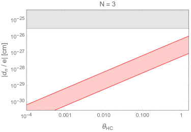
Figure 5: The expected neutron electric dipole moment as a function of the hypercolor vacuum angle $\theta_{\rm HC}$ in models for a composite PNG 750 GeV resonance. For this plot, we choose $N=3$.

It is now straightforward to use our previous results to find the nucleon and electron EDM induced by the above effective interactions. By matching the coefficients of the relevant interactions with the simple model presented in section II, we find the following correspondence:

$$\begin{split}\frac{y_{S}}{m_{\Psi}}\sim\frac{N}{f},\quad\sin 2\alpha\sim\frac{m_{S}^{2}}{\Lambda_{\rm HC}^{2}}\sin{\theta}_{\rm HC},\end{split}$$ (56)

where we have used the relation

$$m_{S}^{2}=(750\,\,{\rm GeV})^{2}\simeq\frac{(m_{\psi}+3m_{\chi})\mu^{3}}{f^{2}}\simeq(m_{\psi}+3m_{\chi})\Lambda_{\rm HC}.$$ (57)

Since the ratio $m_{\Psi}/y_{S}$ should be around 100 GeV to explain the 750 GeV diphoton excess, it turns out that $f\sim N\times 100$ GeV and $\Lambda_{\rm HC}\simeq 4\pi f/\sqrt{N}\sim\sqrt{N}$ TeV, implying that roughly $\sin 2\alpha$ is one or two orders of magnitude smaller than $\theta_{\rm HC}$. In Fig. 5, we depict the neutron EDM in the minimal model for a composite PNG 750 GeV resonance for the parameter region to give $\sigma(pp\rightarrow\gamma\gamma)=1\sim 10$ fb.

The minimal model of Nakai:2015ptz can be generalized or modified to include a hypercolored fermion carrying a nonzero $SU(2)_{L}$ charge Harigaya:2015ezk , e.g. $\chi$ can transform as $(N,1,2)_{Y_{\chi}}$ under $SU(N)_{H}\times SU(3)_{c}\times SU(2)_{L}\times U(1)_{Y}$. Then the hypercolor dynamic with nonzero $\theta_{\rm HC}$ can generate the following CP-odd three $W$-boson operator:

$$\Delta{\cal L}_{\rm CPV}=\frac{N}{16\pi^{2}}\frac{m_{\theta}}{\Lambda_{H}}\frac{\kappa_{W}}{\Lambda_{H}^{2}}\frac{g_{2}^{3}\epsilon_{ijk}}{3}W^{i}_{\mu\rho}W^{j\,\,\rho}_{\nu}\widetilde{W}^{k\,\mu\nu},$$ (58)

where $\kappa_{W}={\cal O}(1)$ according to the NDA rule. Applying our previous result (43) under the relation (56), we find the electron EDM resulting from the above three $W$-boson operator is too small to be observable even when $\theta_{\rm HC}={\cal O}(1)$.

Finally let us note that a composite PNG boson $S$ can have a mixing with the SM Higgs boson if the underlying hypercolor model includes a higher dimensional operator of the form:

$$\frac{1}{\Lambda_{\psi}}|H|^{2}\bar{\psi}_{L}\psi_{R}+\frac{1}{\Lambda_{\chi}}|H|^{2}\bar{\chi}_{L}\chi_{R}+{\rm h.c},$$ (59)

where $\Lambda_{\psi,\chi}$ are complex in general. For instance, this form of dim$-5$ operators can be generated by an exchange of heavy scalar field $\sigma$ which has the couplings

$${\cal L}_{\sigma}=-\frac{1}{2}m_{\sigma}^{2}\sigma^{2}+A_{\sigma}\sigma|H|^{2}+\left(\lambda_{\psi}\sigma\bar{\psi}_{L}\psi_{R}+\lambda_{\chi}\sigma\bar{\chi}_{L}\chi_{R}+{\rm h.c.}\right)+...,$$ (60)

yielding

$$\frac{1}{\Lambda_{\psi}}=\frac{A_{\sigma}\lambda_{\psi}}{m_{\sigma}^{2}},\quad\frac{1}{\Lambda_{\chi}}=\frac{A_{\sigma}\lambda_{\chi}}{m_{\sigma}^{2}}.$$

The resulting $S-H$ mixing angle is estimated as

$$\xi_{SH}\,\sim\,\frac{v\Lambda_{\rm HC}^{2}}{4\pi m_{S}^{2}}\,\frac{{\rm Im}(\Lambda_{\psi,\chi})}{|\Lambda_{\psi,\chi}|^{2}},$$ (61)

where $v=246$ GeV is the vacuum value of the SM Higgs doublet $H$. One can apply this the mixing angle for our previous result (42) to estimate the resulting electron EDM. Note that here $S$ is an approximately pseudoscalar boson, and therefore $\xi_{SH}$ corresponds to a CP-violating mixing angle, while $\sin\alpha$ is CP-conserving and of order unity. One then finds the current bound on the electron EDM implies

$$\frac{\Lambda_{\rm HC}}{|\Lambda_{\psi,\chi}|}\frac{{\rm Im}(\Lambda_{\psi,\chi})}{|\Lambda_{\psi,\chi}|}\,\lesssim\,{\cal O}(10^{-2}).$$ (62)

V Conclusion

The recently announced diphoton excess at 750 GeV in the Run II ATLAS and CMS data may turn out to be the first discovery of new physics beyond the Standard Model at collider experiments. In this paper, we examined the implication of the 750 GeV diphoton excess for the EDM of neutron and electron in models in which the diphoton excess is due to a spin zero resonance $S$ which couples to photons and gluons through the loops of massive vector-like fermions. We found that a neutron EDM comparable to the current experimental bound can be obtained if the CP violating order parameter $\sin 2\alpha$ in the underlying new physics is of ${\cal O}(10^{-1})$. An electron EDM near the present bound can be obtained also when $\sin\xi_{SH}\times\sin\alpha={\cal O}(10^{-3})$, where $\xi_{SH}$ is the mixing angle between $S$ and the SM Higgs boson. For the case that $S$ corresponds to a pseudo-Nambu-Goldstone boson of a QCD-like hypercolor dynamics, one can use the correspondence $\sin 2\alpha\sim m_{S}^{2}\sin\theta_{\rm HC}/\Lambda^{2}_{\rm HC}$ to estimate the resulting EDMs, where $\Lambda_{\rm HC}$ is the scale of spontaneous chiral symmetry breaking by the hypercolor dynamics and $\theta_{\rm HC}$ is the hypercolor vacuum angle. In view of that a nucleon or electron EDM near the current bound can be obtained over a natural parameter region of the model, future precision measurements of the nucleon or electron EDM are highly motivated.

VI Acknowledgment

This work was supported by IBS under the project code, IBS-R018-D1.

References

- (1) ATLAS Collaboration, ATLAS-CONF-2015-081 (2015).
- (2) CMS Collaboration, CMS-PAS-EXO-15-004 (2015).
- (3) M. Delmastro,“Diphoton searches in ATLAS”, Talk at 51st Rencontres de Moriond EW 2016, March 17 (2016).
- (4) P. Musella,“Search for high mass diphoton resonances at CMS”, Talk at 51st Rencontres de Moriond EW 2016, March 17 (2016).
- (5) R. Franceschini et al., JHEP 1603, 144 (2016) [arXiv:1512.04933 [hep-ph]].
- (6) J. E. Kim and G. Carosi, Rev. Mod. Phys. 82, 557 (2010) [arXiv:0807.3125 [hep-ph]].
- (7) S. Weinberg, Phys. Rev. Lett. 63, 2333 (1989).
- (8) S. M. Barr and A. Zee, Phys. Rev. Lett. 65, 21 (1990) Erratum: [Phys. Rev. Lett. 65, 2920 (1990)].
- (9) W. J. Marciano and A. Queijeiro, Phys. Rev. D 33, 3449 (1986).
- (10) F. Boudjema, K. Hagiwara, C. Hamzaoui and K. Numata, Phys. Rev. D 43, 2223 (1991).
- (11) K. Harigaya and Y. Nomura, Phys. Lett. B 754, 151 (2016) [arXiv:1512.04850 [hep-ph]]; JHEP 1603, 091 (2016) [arXiv:1602.01092 [hep-ph]].
- (12) Y. Nakai, R. Sato and K. Tobioka, Phys. Rev. Lett. 116, no. 15, 151802 (2016) [arXiv:1512.04924 [hep-ph]].
- (13) M. Redi, A. Strumia, A. Tesi and E. Vigiani, arXiv:1602.07297 [hep-ph].
- (14) A. Falkowski, O. Slone and T. Volansky, JHEP 1602, 152 (2016) [arXiv:1512.05777 [hep-ph]].
- (15) L. J. Hall, K. Harigaya and Y. Nomura, JHEP 1603, 017 (2016) [arXiv:1512.07904 [hep-ph]].
- (16) H. P. Nilles and M. W. Winkler, arXiv:1604.03598 [hep-ph].
- (17) D. A. Dicus, Phys. Rev. D 41, 999 (1990).
- (18) T. Abe, J. Hisano, T. Kitahara and K. Tobioka, JHEP 1401, 106 (2014) Erratum: [JHEP 1604, 161 (2016)] [arXiv:1311.4704 [hep-ph]].
- (19) M. Jung and A. Pich, JHEP 1404, 076 (2014) [arXiv:1308.6283 [hep-ph]].
- (20) W. Dekens, J. de Vries, J. Bsaisou, W. Bernreuther, C. Hanhart, U. G. Meißner, A. Nogga and A. Wirzba, JHEP 1407, 069 (2014) [arXiv:1404.6082 [hep-ph]].
- (21) G. Degrassi, E. Franco, S. Marchetti and L. Silvestrini, JHEP 0511, 044 (2005) [hep-ph/0510137].
- (22) J. Hisano, K. Tsumura and M. J. S. Yang, Phys. Lett. B 713, 473 (2012) [arXiv:1205.2212 [hep-ph]].
- (23) A. Manohar, H. Georgi, Nucl. Phys. 234, 189 (1984); H. Georgi, Weak Interactions and Modern Particle Theory, Benjamin/Cummings, (Menlo Park, 1984); H. Georgi, L. Randall, Nucl. Phys. 276, 241 (1986).
- (24) M. Pospelov and A. Ritz, Phys. Rev. D 63, 073015 (2001) [hep-ph/0010037].
- (25) J. Hisano, J. Y. Lee, N. Nagata and Y. Shimizu, Phys. Rev. D 85, 114044 (2012) [arXiv:1204.2653 [hep-ph]].
- (26) J. Hisano, D. Kobayashi, W. Kuramoto and T. Kuwahara, JHEP 1511, 085 (2015) [arXiv:1507.05836 [hep-ph]].
- (27) D. A. Demir, M. Pospelov and A. Ritz, Phys. Rev. D 67, 015007 (2003) [hep-ph/0208257].
- (28) K. Cheung, P. Ko, J. S. Lee, J. Park and P. Y. Tseng, arXiv:1512.07853 [hep-ph].
- (29) K. Fuyuto, J. Hisano and N. Nagata, Phys. Rev. D 87, no. 5, 054018 (2013) [arXiv:1211.5228 [hep-ph]].
- (30) C. A. Baker et al., Phys. Rev. Lett. 97, 131801 (2006) [hep-ex/0602020].
- (31) J. Baron et al. [ACME Collaboration], Science 343, 269 (2014) [arXiv:1310.7534 [physics.atom-ph]].
- (32) M. Son and A. Urbano, arXiv:1512.08307 [hep-ph].
- (33) J. Gu and Z. Liu, Phys. Rev. D 93, no. 7, 075006 (2016) [arXiv:1512.07624 [hep-ph]].