Software for cut-generating functions in the Gomory–Johnson model and beyond

Abstract

We present software for investigations with cut generating functions in the Gomory–Johnson model and extensions, implemented in the computer algebra system SageMath.

1 Introduction

Consider the following question from the theory of linear inequalities over the reals: Given a (finite) system $Ax\leq b$, exactly which linear inequalities $\langle a,x\rangle\leq\beta$ are valid, i.e., satisfied for every $x$ that satisfies the given system? The answer is given, of course, by the Farkas Lemma, or, equivalently, by the strong duality theory of linear optimization. As is well-known, this duality theory is symmetric: The dual of a linear optimization problem is again a linear optimization problem, and the dual of the dual is the original (primal) optimization problem.

The question becomes much harder when all or some of the variables are constrained to be integers. The theory of valid linear inequalities here is called cutting plane theory. Over the past 60 years, a vast body of research has been carried out on this topic, the largest part of it regarding the polyhedral combinatorics of integer hulls of particular families of problems. The general theory again is equivalent to the duality theory of integer linear optimization problems. Here the dual objects are not linear, but superadditive (or subadditive) functionals, making the general form of this theory infinite-dimensional even though the original problem started out with only finitely many variables.

These superadditive (or subadditive) functionals appear in integer linear optimization in various concrete forms, for example in the form of dual-feasible functions [1], superadditive lifting functions [12], and cut-generating functions [6].

In the present paper, we describe some aspects of our software [10] for cut-generating functions in the classic 1-row Gomory–Johnson [7, 8] model. In this theory, the main objects are the so-called minimal valid functions, which are the $\mathbb{Z}$-periodic, subadditive functions $\pi\colon\mathbb{R}\to\mathbb{R}_{+}$ with $\pi(0)=0$, $\pi(f)=1$, that satisfy the symmetry condition $\pi(x)+\pi(f-x)=1$ for all $x\in\mathbb{R}$. (Here $f$ is a fixed number.) We refer the reader to the recent survey [4, 5].

Our software is a tool that enables mathematical exploration and research in this domain. It can also be used in an educational setting, where it enables hands-on teaching about modern cutting plane theory based on cut-generating functions. It removes the limitations of hand-written proofs, which would be dominated by tedious case analysis.

The first version of our software [10] was written by the first author, C. Y. Hong, during a Research Experience for Undergraduates in summer 2013. It was later revised and extended by M. Köppe and again by Y. Zhou. The latter added an electronic compendium [11] of extreme functions found in the literature, and added code that handles the case of discontinuous functions. Version 0.9 of our software was released in 2014 to accompany the survey [4, 5]; the software has received continuous updates by the second and third authors since.

Our software is written in Python, making use of the convenient framework of the open-source computer algebra system SageMath [14]. It can be run on a local installation of SageMath, or online via SageMathCloud.

2 Continuous and discontinuous piecewise linear $\mathbb{Z}$-periodic functions

The main objects of our code are the $\mathbb{Z}$-periodic functions $\pi\colon\mathbb{R}\to\mathbb{R}$. Our code is limited to the case of piecewise linear functions, which are allowed to be discontinuous; see the definition below. In the following, we connect to the systematic notation introduced in [3, section 2.1]; see also [4, 5]. In our code, the periodicity of the functions is implicit; the functions are represented by their restriction to the interval $[0,1]$. They can be constructed in various ways using Python functions named piecewise_function_from_breakpoints_and_values etc.; see the source code of the electronic compendium for examples. We also suppress the details of the internal representation; instead we explain the main ways in which the data of the function are accessed.

$\pi$.end_points()

is a list $0=x_{0}<x_{1}<\dots<x_{n-1}<x_{n}=1$ of possible breakpoints of the function in $[0,1]$. In the notation from [3, 4, 5], these endpoints are extended periodically as $B=\{\,x_{0}+t,x_{1}+t,\dots,x_{n-1}+t:t\in\mathbb{Z}\,\}$. Then the set of 0-dimensional faces is defined to be the collection of singletons, $\bigl{\{}\,\{x\}:x\in B\,\bigr{\}}$, and the set of one-dimensional faces to be the collection of closed intervals, $\bigl{\{}\,[x_{i}+t,x_{i+1}+t]:i=0,\dots,{n-1}\text{ and }t\in\mathbb{Z}\,\bigr{\}}.$ Together, we obtain $\mathcal{P}=\mathcal{P}_{B}$, a locally finite polyhedral complex, periodic modulo $\mathbb{Z}$.

$\pi$.values_at_end_points()

is a list of the function values $\pi(x_{i})$, $i=0,\dots,n$. This list is most useful for continuous piecewise linear functions, as indicated by $\pi$.is_continuous(), in which case the function is defined on the intervals $[x_{i},x_{i+1}]$ by linear interpolation.

$\pi$.limits_at_end_points()

provides data for the general, possibly discontinuous case in the form of a list limits of 3-tuples, with

limits[$$i =\pi(x_{i})$$][0]

limits[$$i =\pi(x_{i}^{+})=\lim_{x\to x_{i},x>x_{i}}\pi(x)$$][1]

limits[$$i =\pi(x_{i}^{-})=\lim_{x\to x_{i},x<x_{i}}\pi(x).$$][-1]

The function is defined on the open intervals $(x_{i},x_{i+1})$ by linear interpolation of the limit values $\pi(x_{i}^{+})$, $\pi(x_{i+1}^{-})$.

$\pi$($x$) and $\pi$.limits($x$)

evaluate the function at $x$ and provide the 3-tuple of its limits at $x$, respectively.

$\pi$.which_function($x$)

returns a linear function, denoted $\pi_{I}\colon\mathbb{R}\to\mathbb{R}$ in [3, 4, 5], where $I$ is the smallest face of $\mathcal{P}$ containing $x$, so $\pi(x)=\pi_{I}(x)$ for $x\in\operatorname{rel\,int}(I)$.

Functions can be plotted using the standard SageMath function plot($\pi$), or using our function plot_with_colored_slopes($\pi$), which assigns a different color to each different slope value that a linear piece takes. Examples of such functions are shown in Figures 2 and 3.

3 The diagrams of the decorated 2-dimensional polyhedral complex $\Delta\mathcal{P}$

We now describe certain 2-dimensional diagrams which record the subadditivity and additivity properties of a given function. These diagrams, in the continuous case, have appeared extensively in [4, 5, 11]. An example for the discontinuous case appeared in [11]. We have engineered these diagrams from earlier forms that can be found in [9] (for the discussion of the merit_index) and in [3], to become power tools for the modern cutgeneratingfunctionologist. Not only is the minimality of a given function immediately apparent on the diagram, but also the extremality proof for a given class of piecewise minimal valid functions follows a standard pattern that draws from these diagrams. See [5, prelude] and [11, sections 2 and 4] for examples of such proofs.

3.1 The polyhedral complex and its faces

Following [3, 4, 5], we introduce the function

$$\Delta\pi\colon\mathbb{R}\times\mathbb{R}\to\mathbb{R},\quad\Delta\pi(x,y)=\pi(x)+\pi(y)-\pi(x+y),$$

which measures the slack in the subadditivity condition. Thus, if $\Delta\pi(x,y)<0$, subadditivity is violated at $(x,y)$; if $\Delta\pi(x,y)=0$, additivity holds at $(x,y)$; and if $\Delta\pi(x,y)>0$, we have strict subadditivity at $(x,y)$. The piecewise linearity of $\pi(x)$ induces piecewise linearity of $\Delta\pi(x,y)$. To express the domains of linearity of $\Delta\pi(x,y)$, and thus domains of additivity and strict subadditivity, we introduce the two-dimensional polyhedral complex $\Delta\mathcal{P}$. The faces $F$ of the complex are defined as follows. Let $I,J,K\in\mathcal{P}$, so each of $I,J,K$ is either a breakpoint of $\pi$ or a closed interval delimited by two consecutive breakpoints. Then

$$F=F(I,J,K)=\left\{\,(x,y)\in\mathbb{R}\times\mathbb{R}\,:\,x\in I,\,y\in J,\,x+y\in K\,\right\}.$$

In our code, a face is represented by an instance of the class Face. It is constructed from $I,J,K$ and is represented by the list of vertices of $F$ and its projections $I^{\prime}=p_{1}(F)$, $J^{\prime}=p_{2}(F)$, $K^{\prime}=p_{3}(F)$, where $p_{1},p_{2},p_{3}\colon\mathbb{R}\times\mathbb{R}\to\mathbb{R}$ are defined as $p_{1}(x,y)=x$, $p_{2}(x,y)=y$, $p_{3}(x,y)=x+y$. The vertices $\operatorname{vert}(F)$ are obtained by first listing the basic solutions $(x,y)$ where $x$, $y$, and $x+y$ are fixed to endpoints of $I$, $J$, and $K$, respectively, and then filtering the feasible solutions. The three projections are then computed from the list of vertices. Due to the $\mathbb{Z}$-periodicity of $\pi$, we can represent a face as a subset of $[0,1]\times[0,1]$. See Figure 1 for an example. Because of the importance of the projection $p_{3}(x,y)=x+y$, it is convenient to imagine a third, $(x+y)$-axis in addition to the $x$-axis and the $y$-axis, which traces the bottom border for $0\leq x+y\leq 1$ and then the right border for $1\leq x+y\leq 2$. To make room for this new axis, the $x$-axis should be drawn on the top border of the diagram.

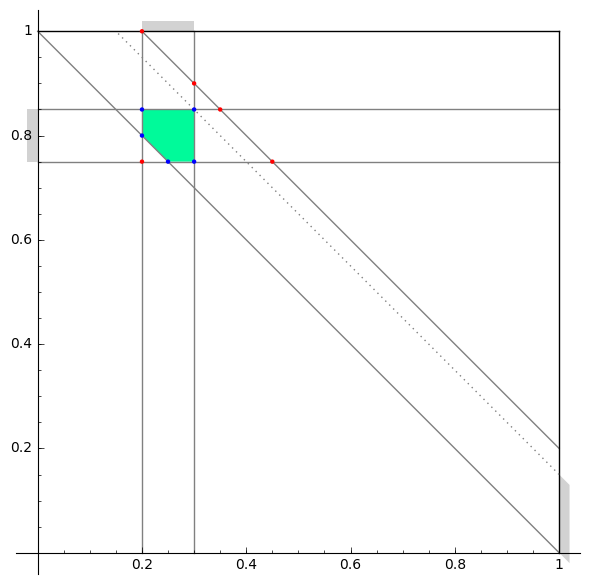
Figure 1: An example of a face $F=F(I,J,K)$ of the 2-dimensional polyhedral complex $\Delta\mathcal{P}$, set up by F = Face([[0.2, 0.3], [0.75, 0.85], [1, 1.2]]). It has vertices (blue) $(0.2,0.85),(0.3,0.75),(0.3,0.85),(0.2,0.8),(0.25,0.75)$, whereas the other basic solutions (red) $(0.2,0.75),(0.2,1),(0.3,0.9),(0.35,0.85),(0.45,0.75)$ are filtered out because they are infeasible. The face $F$ has projections (gray shadows) $I^{\prime}=p_{1}(F)=[0.2,0.3]$ (top border), $J^{\prime}=p_{2}(F)=[0.75,0.85]$ (left border), and $K^{\prime}=p_{3}(F)=[1,1.15]$ (right border). Note that $K^{\prime}\subsetneq K$.

3.2 plot_2d_diagram_with_cones

We now explain the first version of the 2-dimensional diagrams, plotted by the function plot_2d_diagram_with_cones($\pi$); see Figure 2.

Figure 2: Two diagrams of functions and their polyhedral complexes $\Delta\mathcal{P}$ with colored cones at $\operatorname{vert}(\Delta\mathcal{P})$, as plotted by the command plot_2d_diagram_with_cones(h). Left, continuous function h = not_minimal_2(). Right, a random discontinuous function generated by h = random_piecewise_function(xgrid=5, ygrid=5, continuous_proba=1/3, symmetry=True).

At the border of these diagrams, the function $\pi$ is shown twice (blue), along the $x$-axis (top border) and along the $y$-axis (left border). The solid grid lines in the diagrams are determined by the breakpoints of $\pi$: vertical, horizontal and diagonal grid lines correspond to values where $x$, $y$ and $x+y$ are breakpoints of $\pi$, respectively. The vertices of the complex $\Delta\mathcal{P}$ are the intersections of these grid lines.

In the continuous case, we indicate the sign of $\Delta\pi(x,y)$ for all vertices by colored dots on the diagram: red indicates $\Delta\pi(x,y)<0$ (subadditivity is violated); green indicates $\Delta\pi(x,y)=0$ (additivity holds).

Example 1

In Figure 2 (left), the vertex $(x,y)=(\frac{1}{5},\frac{3}{5})$ is marked green, since

$$\Delta\pi(\tfrac{1}{5},\tfrac{3}{5}) =\pi(\tfrac{1}{5})+\pi(\tfrac{3}{5})-\pi(\tfrac{4}{5})=\tfrac{1}{5}+\tfrac{4}{5}-1=0.$$

In the discontinuous case, beside the subadditivity slack $\Delta\pi(x,y)$ at a vertex $(x,y)$, one also needs to study the limit value of $\Delta\pi$ at the vertex $(x,y)$ approaching from the interior of a face $F\in\Delta\mathcal{P}$ containing the vertex $(x,y)$. This limit value is defined by

$$\Delta\pi_{F}(x,y)=\lim_{\begin{subarray}{c}(u,v)\to(x,y)\\ (u,v)\in\operatorname{rel\,int}(F)\end{subarray}}\Delta\pi(u,v),\quad\text{where }F\in\Delta\mathcal{P}\text{ such that }(x,y)\in F.$$

We indicate the sign of $\Delta\pi_{F}(x,y)$ by a colored cone inside $F$ pointed at the vertex $(x,y)$ on the diagram. There could be up to $12$ such cones (including rays for one-dimensional $F$) around a vertex $(x,y)$.

Example 2

In Figure 2 (right), the lower right corner $(x,y)=(\frac{2}{5},\frac{4}{5})$ of the face $F=F(I,J,K)$ with $I=[\frac{1}{5},\frac{2}{5}]$, $J=[\frac{4}{5},1]$, $K=[1,\frac{6}{5}]$ is green, since

$$\Delta\pi_{F}(x,y) =\lim_{\begin{subarray}{c}(u,v)\to(\frac{2}{5},\frac{4}{5})\\ (u,v)\in\operatorname{rel\,int}(F)\end{subarray}}\Delta\pi(u,v)$$

$$=\lim_{u\to\frac{2}{5},\;u<\frac{2}{5}}\pi(u)+\lim_{v\to\frac{4}{5},\;v>\frac{4}{5}}\pi(v)-\lim_{w\to\frac{6}{5},\;w<\frac{6}{5}}\pi(w)$$

$$=\pi(\tfrac{2}{5}^{-})+\pi(\tfrac{4}{5}^{+})-\pi(\tfrac{1}{5}^{-})\quad\text{(as }\pi(\tfrac{6}{5}^{-})=\pi(\tfrac{1}{5}^{-})\text{ by periodicity)}$$

$$=0+1-1=0.$$

The horizontal ray to the left of the same vertex $(x,y)=(\frac{2}{5},\frac{4}{5})$ is red, because approaching from the one-dimensional face $F^{\prime}=F(I^{\prime},J^{\prime},K^{\prime})$ that contains $(x,y)$, with $I^{\prime}=[\frac{1}{5},\frac{2}{5}]$, $J^{\prime}=\{\frac{4}{5}\}$, $K^{\prime}=[1,\frac{6}{5}]$, we have the limit value

$$\Delta\pi_{F^{\prime}}(x,y)=\lim_{\begin{subarray}{c}(u,v)\to(\frac{2}{5},\frac{4}{5})\\ (u,v)\in\operatorname{rel\,int}(F^{\prime})\end{subarray}}\Delta\pi(u,v)=\lim_{\begin{subarray}{c}u\to\frac{2}{5}\\ u<\frac{2}{5}\end{subarray}}\pi(u)+\pi(\tfrac{4}{5})-\lim_{\begin{subarray}{c}w\to\frac{6}{5}\\ w<\frac{6}{5}\end{subarray}}\pi(w)=0+\tfrac{3}{5}-1<0.$$

3.3 plot_2d_diagram and additive faces

Now assume that $\pi$ is a subadditive function. Then there are no red dots or cones on the above diagram of the complex $\Delta\mathcal{P}$. See Figure 3.

For a continuous subadditive function $\pi$, we say that a face $F\in\Delta\mathcal{P}$ is additive if $\Delta\pi=0$ over all $F$. Note that $\Delta\pi$ is affine linear over $F$, and so the face $F$ is additive if and only if $\Delta\pi(x,y)=0$ for all $(x,y)\in\operatorname{vert}(F)$. It is clear that any subface $E$ of an additive face $F$ ($E\subseteq F$, $E\in\Delta\mathcal{P}$) is still additive. Thus the additivity domain of $\pi$ can be represented by the list of inclusion-maximal additive faces of $\Delta\mathcal{P}$; see [4, Lemma 3.12].

Figure 3: Diagrams of $\Delta\mathcal{P}$ of a discontinuous function h = hildebrand_2_sided_discont_2_slope_1(), with (left) additive limiting cones as plotted by the command plot_2d_diagram_with_cones(h); (right) additive faces as plotted by the command plot_2d_diagram(h).

For a discontinuous subadditive function $\pi$, we say that a face $F\in\Delta\mathcal{P}$ is additive if $F$ is contained in a face $F^{\prime}\in\Delta\mathcal{P}$ such that $\Delta\pi_{F^{\prime}}(x,y)=0$ for any $(x,y)\in F$. Since $\Delta\pi$ is affine linear in the relative interiors of each face of $\Delta\mathcal{P}$, the last condition is equivalent to $\Delta\pi_{F^{\prime}}(x,y)=0$ for any $(x,y)\in\operatorname{vert}(F)$. Depending on the dimension of $F$, we do the following.

1. Let $F$ be a two-dimensional face of $\Delta\mathcal{P}$. If $\Delta\pi_{F}(x,y)=0$ for any $(x,y)\in\operatorname{vert}(F)$, then $F$ is additive. Visually on the 2d-diagram with cones, each vertex of $F$ has a green cone sitting inside $F$.

2. Let $F$ be a one-dimensional face, i.e., an edge of $\Delta\mathcal{P}$. Let $(x_{1},y_{1}),(x_{2},y_{2})$ be its vertices. Besides $F$ itself, there are two other faces $F_{1},F_{2}\in\Delta\mathcal{P}$ that contain $F$. If $\Delta\pi_{F^{\prime}}(x_{1},y_{1})=\Delta\pi_{F^{\prime}}(x_{2},y_{2})=0$ for $F^{\prime}=F$, $F_{1}$, or $F_{2}$, then the edge $F$ is additive.

3. Let $F$ be a zero-dimensional face of $\Delta\mathcal{P}$, $F=\{(x,y)\}$. If there is a face $F^{\prime}\in\Delta\mathcal{P}$ such that $(x,y)\in F^{\prime}$ and $\Delta\pi_{F^{\prime}}(x,y)=0$, then $F$ is additive. Visually on the 2d-diagram with cones, the vertex $(x,y)$ is green or there is a green cone pointing at $(x,y)$.

On the diagram Figure 3 (right), the additive faces are shaded in green. The projections $p_{1}(F)$, $p_{2}(F)$, and $p_{3}(F)$ of a two-dimensional additive face $F$ are shown as gray shadows on the $x$-, $y$- and $(x+y)$-axes of the diagram, respectively.

4 Additional functionality

minimality_test($\pi$)

implements a fully automatic test whether a given function is a minimal valid function, using the information that the described 2-dimensional diagrams visualize. The algorithm is equivalent to the one described, in the setting of discontinuous pseudo-periodic superadditive functions, in Richard, Li, and Miller [13, Theorem 22].

extremality_test($\pi$)

implements a grid-free generalization of the automatic extremality test from [3], which is suitable also for piecewise linear functions with rational breakpoints that have huge denominators. Its support for functions with algebraic irrational breakpoints such as bhk_irrational [3, section 5] is experimental and will be described in a forthcoming paper.

generate_covered_intervals($\pi$)

computes connected components of covered (affine imposing [3]) intervals. This is an ingredient in the extremality test.

extreme_functions

is the name of a Python module that gives access to the electronic compendium of extreme functions; see [11] and [4, Tables 1–4].

procedures

provides transformations of extreme functions; see [4, Table 5].

random_piecewise_function()

generates a random piecewise linear function with prescribed properties, to enable experimentation and exploration.

demo.sage

demonstrates further functionality and the use of the help system.

References

- [1] C. Alves, F. Clautiaux, J. V. de Carvalho, and J. Rietz, Dual-feasible functions for integer programming and combinatorial optimization: Basics, extensions and applications, EURO Advanced Tutorials on Operational Research, Springer, 2016, doi:10.1007/978-3-319-27604-5, ISBN 978-3-319-27602-1.
- [2] A. Basu, M. Conforti, M. Di Summa, and J. Paat, Extreme functions with an arbitrary number of slopes, to appear in Proc. IPCO 2016, available from http://www.ams.jhu.edu/~abasu9/papers/infinite-slopes.pdf.
- [3] A. Basu, R. Hildebrand, and M. Köppe, Equivariant perturbation in Gomory and Johnson’s infinite group problem. I. The one-dimensional case, Mathematics of Operations Research 40 (2014), no. 1, 105–129, doi:10.1287/moor.2014.0660.
- [4] , Light on the infinite group relaxation I: foundations and taxonomy, 4OR (2015), 1–40, doi:10.1007/s10288-015-0292-9.
- [5] , Light on the infinite group relaxation II: sufficient conditions for extremality, sequences, and algorithms, 4OR (2015), 1–25, doi:10.1007/s10288-015-0293-8.
- [6] M. Conforti, G. Cornuéjols, A. Daniilidis, C. Lemaréchal, and J. Malick, Cut-generating functions and S-free sets, Mathematics of Operations Research 40 (2013), no. 2, 253–275, http://dx.doi.org/10.1287/moor.2014.0670.
- [7] R. E. Gomory and E. L. Johnson, Some continuous functions related to corner polyhedra, I, Mathematical Programming 3 (1972), 23–85, doi:10.1007/BF01584976.
- [8] , Some continuous functions related to corner polyhedra, II, Mathematical Programming 3 (1972), 359–389, doi:10.1007/BF01585008.
- [9] , T-space and cutting planes, Mathematical Programming 96 (2003), 341–375, doi:10.1007/s10107-003-0389-3.
- [10] C. Y. Hong, M. Köppe, and Y. Zhou, Sage program for computation and experimentation with the -dimensional Gomory–Johnson infinite group problem, 2014, available from https://github.com/mkoeppe/infinite-group-relaxation-code.
- [11] M. Köppe and Y. Zhou, An electronic compendium of extreme functions for the Gomory–Johnson infinite group problem, Operations Research Letters 43 (2015), no. 4, 438–444, doi:10.1016/j.orl.2015.06.004.
- [12] Q. Louveaux and L. A. Wolsey, Lifting, superadditivity, mixed integer rounding and single node flow sets revisited, Quarterly Journal of the Belgian, French and Italian Operations Research Societies 1 (2003), no. 3, 173–207, doi:10.1007/s10288-003-0016-4.
- [13] J.-P. P. Richard, Y. Li, and L. A. Miller, Valid inequalities for MIPs and group polyhedra from approximate liftings, Mathematical Programming 118 (2009), no. 2, 253–277, doi:10.1007/s10107-007-0190-9.
- [14] W. A. Stein et al., Sage Mathematics Software (Version 7.1), The Sage Development Team, 2016, http://www.sagemath.org.