Constrained Nonlinear and Mixed Effects Differential Equation Models for Dynamic Cell Polarity Signaling

Author’s Footnote:

Zhen Xiao was a PhD student in the Department of Statistics at University of California, Riverside. He is now a senior biosatistician at Biogen Inc, Cambridge, MA, 02142 (email: nehzxiao@gmail.com); and Nicolas Brunel is an associate professor in ENSIIE & Laboratoire de Mathématiques et Modélisation d’Evry UMR CNRS 8071, Universite d’Evry, France (email: nicolas.brunel@ensiie.fr); and Zhenbiao Yang is a professor in the Department of Botany and Plant Sciences and the Center for Plant Cell Biology and Institute for Integrative Genome Biology at University of California, Riverside, CA 92521, USA (email: zhenbiao.yang@ucr.edu); and Xinping Cui is a professor in the Department of Statistics and the Center for Plant Cell Biology and Institute for Integrative Genome Biology at University of California, Riverside, CA 92521, USA (email: xinping.cui@ucr.edu). This work was partially supported by UC Riverside AES-CE RSAP A01869.

Abstract

The key of tip growth in eukaryotes is the polarized distribution on plasma membrane of a particle named ROP1. This distribution is the result of a positive feedback loop, whose mechanism can be described by a Differential Equation parametrized by two meaningful parameters $k_{pf}$ and $k_{nf}$. We introduce a mechanistic Integro-Differential Equation (IDE) derived from a spatiotemporal model of cell polarity and we show how this model can be fitted to real data i.e. ROP1 intensities measured on pollen tubes. At first, we provide an existence and uniqueness result for the solution of our IDE model under certain conditions. Interestingly, this analysis gives a tractable expression for the likelihood, and our approach can be seen as the estimation of a constrained nonlinear model. Moreover, we introduce a population variability by a constrained nonlinear mixed model. We then propose a constrained Least Squares method to fit the model for the single pollen tube case, and two methods, constrained Methods of Moments and constrained Restricted Maximum Likelihood (REML) to fit the model for the multiple pollen tubes case. The performances of all three methods are studied through simulations and are used on an in-house multiple pollen tubes dataset generated at UC Riverside.

Keywords: Constrained Mixed effects model, Restricted maximum likelihood, Semilinear-linear Elliptic Differential Equation, Integro-Differential Equation, Cell Polarity.

1. Introduction

Cell polarity is a fundamental feature of almost all cells. It is required for the differentiation of new cells, the formation of cell shapes, and cell migration, etc. Pollen tubes, which extend by an extreme form of polar growth (termed tip growth) to deliver sperms to the ovary for fertilization, are one of the fastest growing cells in plants and therefore represent an attractive model system to investigate polarized cell growth (Yang, 1998; Hepler et al., 2001; Lee and Yang, 2008; Yang, 2008; Qin and Yang, 2011).

When pollen grain is activated by a certain internal or external stimulus, the signaling molecule GTPase ROP1 in the cytosol will be activated and translocated onto the plasma membrane, forming an apical ROP1 cap. Once maintained, the apical ROP1 cap will trigger exocytosis, leading to cell growth at the site of the apical cap. Figure 1 shows the three main stages of pollen tube tip growth: polarity establishment of the signaling molecule GTPase ROP1 (i.e, active ROP1s form a apical cap), exocytosis to increase cell membrane surface and deliver cell wall materials, and cell wall extension.

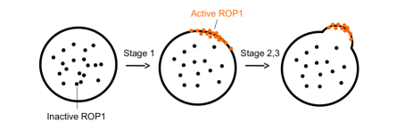
Figure 1: Three main stages of tip growth of pollen tubes. Stage 1: ROP1 polarity establishment; Stage 2: Pectin Exocytosis; Stage 3: Cell wall extension.

Several mathematical models have been built to simulate pollen tube tip growth (Dumais et al., 2006; J. H. Kroeger, 2008; Campas and Mahadevan, 2009; Lowery and Vanvactor, 2009; Fayant et al., 2010). These models focused on the cell wall mechanics and the cell wall mechanics-mediated shape formation of pollen tubes. However, it has been found that the generation of apical cap of active ROP1 at stage 1 plays a predominant role in determining polarity of the pollen tube (Lin et al., 1996; Li et al., 1998). Therefore, modeling the distribution of ROP1s on the membrane is the key to understand the tip growth of pollen tube. As a key regulator of the self-organizing pollen tube system, the activity and distribution of ROP1 are fine-tuned by both positive and negative feedback mechanisms (Hwang et al., 2010) as well as slow diffusion shown in Figure 2. Altschuler et al. (2008) proposed a linear differential equation model for the polarization of the GTPase Cdc42 in budding yeast but only considered positive feedback. On the other hand, for all the aforementioned models attention has been paid to predict or simulate the output using these models with given parameters. Less efforts have been devoted to the inverse problem, i.e., using the experimental data to estimate the parameters that characterize these models (Ramsay et al., 2007; Wu and Chen, 2008; Brunel, 2008; Brunel et al., 2014).

In this paper, we propose an integro-ordinary differential equation (IDE) model to describe the three processes together (positive feedback, negative feedback and diffusion) that lead to ROP1 polarity formation at steady state. Our main interest lies in the inverse problem of estimating the parameters for the positive feedback and the negative feedback. However, two identifiability issues arise in the context of our model. The first identifiability problem is whether the solution to the nonlinear IDE model exists and is unique. We will show that the IDE model is closely related to a semilinear elliptic equation, from which we establish the original theory on the existence and uniqueness of solutions to this type of IDE. The second identifiability problem is whether the observed data is enough to identify the parameters in the IDE model. By applying the identifiability analysis methods suggested by Miao et al. (2011), we can prove that the two parameters of interest are identifiable.

Solving the identifiability problems allows us to derive an admissible parameter space inside which the solution to the IDE model exists. The IDE model can then be re-parametrized as a mixed-effects differential equation model with linear constraints over the admissible parameter space. In statistical literature, there exist a number of papers for mixed-effects differential equation models. Li et al. (2002) proposed to estimate time-varying parameters in the mixed-effects ordinary differential equations by maximizing the double penalized log likelihood. Putter et al. (2002) proposed a hierarchical Bayesian approach for estimating population parameters in a system of mixed-effects nonlinear differential equations that have closed-form solutions. Guedj et al. (2007) extended this system of mixed-effects nonlinear differential equations for which no closed form is available. They proposed to estimate both population and individual parameters in this extended model by a maximum likelihood approach using a Newton-like algorithm. Huang and Wu (2006a) and Huang and Wu (2006b) developed a hierarchical Bayesian approach to estimate both population and individual dynamic parameters in a set of mixed-effects nonlinear differential equations which have no closed-form solutions. Lu et al. (2011) employed stochastic approximation EM approach for parameter estimation of mixed-effects ordinary differential equations.

However, parameter estimation problems for mixed-effects differential equation models with linear inequality constraints have not been investigated. In this paper, we propose two algorithms based on modified REML and Method of Moments (MM) approaches (Lu and Meeker, 1993) to estimate the parameters with constraints in a mixed-effects differential equation model. The constrained estimators are shown to be consistent and the methodology we propose is quite general and can be applied to many mixed-effects ODE settings with little modification.

The paper is organized as follows. In section 2, we introduce the IPDE and IDE model motivated by the GTPbase ROP1 polarization process. In the next section, we give sufficient and necessary conditions for existence and uniqueness of a positive solution to the IDE model, and we derive a tractable generic expression for solutions of the IDE. In section 4, we introduce the IDE based nonlinear statistical model with linear constraint for a single pollen tube. We then extend the model for multiple pollen tubes and re-parametrize it as a nonlinear mixed model with linear constraints. The two estimators of Constrained Method of Moments (CMM) and Constrained REML(CREML) are proposed and the asymptotic properties of CMM are discussed. We examine the performance of the proposed estimation procedures through simulation studies in section 5 and real data analysis in section 6. We conclude the paper in section 7.

2. An Integral-Differential Equation Model of Cell Polarity

To build the cell-signaling model of ROP1 polarity formation and maintenance, we assume that the redistribution of signaling molecules is determined by three fundamental transport mechanisms including (1) A positive feedback loop with rate $k_{pf}$ mediated by exocytosis and ROP1 activators such as RopGEFs (Kost et al., 1999; Li et al., 1999; Berken et al., 2005; Gu et al., 2005; Lee et al., 2008; McKenna et al., 2009); (2) A global negative regulation with rate $k_{nf}$ mediated by cytosolic ROP1 inhibitors such as RopGAPs (Hwang et al., 2008); (3) Slow lateral diffusion of ROP1 protein on apical plasma membrane with rate $D$. These three processes are shown in Figure 2. The following semilinear Integro-Partial Differential Equation describes how these three processes together lead to ROP1 polarity formation:

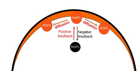
Figure 2: ROP1 polarity formation is determined by positive feedback, negative feedback and lateral diffusion process.

$$\left\{\begin{array}[]{l}\frac{\partial R(x,t)}{\partial t}=k_{pf}R(x,t)^{\alpha}(1-\frac{\int_{-L_{0}}^{L_{0}}{R(x,t)dx}}{R_{tot}})-k_{nf}R(x,t)+D\nabla^{2}R(x,t)\\ \text{where }\qquad\{x,t\}\in[-L_{0},L_{0}]\times[0,\infty],\qquad R(-L_{0},t)=R(L_{0},t)=0\end{array}\right.$$ (1)

$R(x,t)$ denotes the ROP1 intensity in position $x$ on the membrane at time $t$, which can be observed at a oblique plane of total length $2L_{0}$ passing through the cell center. $R_{tot}$ denotes the total free ROP1 in the cell. Throughout this paper, $R_{tot}$, $D$, $\alpha>1$ and $L_{0}$ are assumed to be known constants. This model is similar as the PDE model described in Altschuler et al. (2008) except in their model spontaneous association was included, the fraction of all particles on the membrane is specified as $\frac{\int_{-L_{0}}^{L_{0}}{R(x,t)dx}}{R_{tot}}$ and $\alpha$ was assumed to be 1.

At equilibrium $t_{0}$, $\frac{\partial R(x,t)}{\partial t}|_{t=t_{0}}=0$, $i.e.$, the ROP1 density won’t change with time. From now on, we write $R(x,t_{0})$ as $R(x)$. The IPDE model (1) then degenerates to the following IDE model

$$\left\{\begin{array}[]{ll}-D\partial_{x}^{2}R=-k_{nf}R+k_{pf}R^{\alpha}(1-\frac{\int_{-L_{0}}^{L_{0}}{Rdx}}{R_{tot}})\\ \text{where }\qquad x\in[-L_{0},L_{0}],\qquad R(-L_{0})=R(L_{0})=0\end{array}\right.$$ (2)

Our interest lies in the estimation of the parameters for $k_{pf}$ and $k_{nf}$. However, two issues immediately arise, namely, the existence and uniqueness of the solution $R$ to the equation (2) and the identifiability of $k_{pf}$ and $k_{nf}$. Section 3 is devoted to address these two issues.

3. Identifiability Analysis

In this section, we first show that the solution $R$ to the equation (2) exists and is unique. To the best of our knowledge, this is the first study on the existence and uniqueness of solution to integral differential equations when $\alpha\geq 1$. We then apply the identifiability analysis suggested by Miao et al. (2011) and verified that parameters $k_{pf}$ and $k_{nf}$ are identifiable.

3.1 Existence and Uniqueness of Solution $R$

Lemma 1.

For all $c\in(0,\infty]$, there exists an unique positive solution $\sigma_{0}(x)$ to (3) with Dirichlet conditions on $[-c,c]$.

$$\left\{\begin{array}[]{ll}-\partial_{x}^{2}u=-u+u^{\alpha}&x\in[-c,c]\\ u(-c)=u(c)=0\end{array}\right.$$ (3)

Moreover, $\sigma_{0}(x)$ is positive, even and increasing at $[-c,0]$ and decreasing at $[0,c]$.

Lemma 2.

For all $\lambda^{{}^{\prime}}>0$, there exists an unique positive solution $R_{\lambda^{\prime}}(x)$ to (4) with Dirichlet conditions on $\Omega=\left[-L_{0},L_{0}\right]$, where $L_{0}\in(0,\infty]$.

$$\left\{\begin{array}[]{ll}-D\partial_{x}^{2}u=-k_{nf}u+\lambda^{\prime}k_{pf}u^{\alpha}\\ \text{where }\qquad x\in[-L_{0},L_{0}],\qquad u(-L_{0})=u(L_{0})=0\end{array}\right.$$ (4)

Moreover, if $\sigma_{0}(x)$ is the unique positive solution to (3) defined on $\Omega^{\prime}=\left[-L_{0}\sqrt{\frac{k_{nf}}{D}},L_{0}\sqrt{\frac{k_{nf}}{D}}\right]$, then

$$R_{\lambda^{\prime}}(x)=\left(\frac{k_{pf}}{k_{nf}}\lambda^{\prime}\right)^{\frac{1}{1-\alpha}}\sigma_{0}(\sqrt{\frac{k_{nf}}{D}}x)\doteq R_{\lambda,\mu}(x)=\lambda\sigma_{0}(\mu x).$$ (5)

Where $\lambda=(\frac{k_{pf}}{k_{nf}}\lambda^{{}^{\prime}})^{\frac{1}{1-\alpha}}$, and $\mu=\sqrt{\frac{k_{nf}}{D}}$.

The proofs of Lemma 1 and 2 are provided in the Appendix. It is easy to see that if there exists a unique positive solution $R_{\lambda^{\prime}}(x)$ to equation (4) such that $\lambda^{{}^{\prime}}=1-\frac{\int_{x}R_{\lambda^{\prime}}(x)dx}{R_{tot}}$ , then $R_{\lambda^{\prime}}(x)$ is also a solution to equation (2). In the following, we provide sufficient and necessary conditions that solutions to equation (4) are also solutions to equation (2).

Sufficient Condition: Let $\sigma_{0}$ be the positive solution to (3) on $\Omega^{\prime}=\left[-L_{0}\sqrt{\frac{k_{nf}}{D}},L_{0}\sqrt{\frac{k_{nf}}{D}}\right]$. Consider the family of function $R_{\lambda,\mu}(x)$ defined in (5) and the discriminant function

$$\Lambda(k_{nf},k_{pf},D,R_{tot},\sigma_{0})=\frac{k_{nf}}{k_{pf}}-\frac{1}{\alpha}\left(\frac{\alpha-1}{\alpha}\sqrt{\frac{k_{nf}}{D}}\frac{R_{tot}}{\left\|\sigma_{0}\right\|_{1}}\right)^{\alpha-1}$$ (6)

If $\Lambda(k_{nf},k_{pf},D,R_{tot},\sigma_{0})=0(<0)$, then one (two) positive solution(s) to (2) can be found in the family of function $R_{\lambda,\mu}(x)$.

Necessary Condition: Any positive solution to (2) can be written in the form $R_{\lambda,\mu}(x)=\lambda\sigma_{0}(\mu x)$.

Remark 1.

The proofs of sufficient condition and necessary condition are provided in the Appendix. As a result, the solution $R$ to (2) can be obtained as following when the values of $k_{nf}$ and $k_{pf}$ are given

1. Solve the semilinear elliptic equation (3) on $\Omega^{\prime}=\left[-L_{0}\sqrt{\frac{k_{nf}}{D}},L_{0}\sqrt{\frac{k_{nf}}{D}}\right]$.

2. Compute $\left\|\sigma_{0}\right\|_{1}$ and the discriminant function $\Lambda(k_{nf},k_{pf},D,R_{tot},\sigma_{0})$.

3. If $\Lambda(k_{nf},k_{pf},D,R_{tot},\sigma_{0})=0$, find the positive roots $\lambda^{*}$ of $g(\lambda)$ (defined in the Appendix section A.3), and compute the solution $R_{\lambda^{*},\mu}(x)$.

4. If $\Lambda(k_{nf},k_{pf},D,R_{tot},\sigma_{0})<0$, find the positive roots $\lambda_{1}^{*}$ and $\lambda_{2}^{*}$ of $g(\lambda)$ (defined in the Appendix section A.3), and compute the solutions $R_{\lambda_{1}^{*},\mu}(x)$ and $R_{\lambda_{2}^{*},\mu}(x)$.

In practice, the solution closer to the experimental data should be chooen if there are two solutions.

Remark 2.

For $\lambda>0$, the solution $R_{\lambda,\mu}(x)$ to (2) is a positive and even function. Moreover, it increases at $\left[-L_{0},0\right]$ and decreases at $\left[0,L_{0}\right]$, and the maximum $R_{\lambda,\mu}(0)=\max_{x\in\Omega}R_{\lambda,\mu}(x)>\lambda$. The proof is provided in the Appendix. It will be shown later in section 7 that the ROP data reflects these qualitative properties.

Remark 3.

From sufficient condition, we see that the solution of (2) is determined by two parameters, $\mu$ and $\lambda$, which can be seen as a reparametrization of $k_{nf}$ and $k_{pf}$. Hence, (2) is not over parametrized by $k_{nf}$ and $k_{pf}$.

3.2. Identifiability of $k_{nf}$ and $k_{pf}$

In this section, we prove that the parameters of interest $k_{nf}$ and $k_{pf}$ are globally identifiable and therefore are locally strongly identifiable.

Let $R(x)$ denote the solution to (2). In practice, $R(x)$ is a positive and non-constant function on interval $[-L_{0},L_{0}]\subset[-L,L]$. Suppose for parameters $(k_{nf}^{0},k_{pf}^{0})$ and $(k_{nf}^{1},k_{pf}^{1})$, $R(x;k_{nf}^{0},k_{pf}^{0})=R(x;k_{nf}^{1},k_{pf}^{1})$ on $[-L_{0},L_{0}]$, then we have

$$k_{nf}^{0}R(x)-k_{pf}^{0}R^{\alpha}(x)\left(1-\frac{\int_{-L}^{L}R(x)dx}{R_{tot}}\right)=k_{nf}^{1}R(x)-k_{pf}^{1}R^{\alpha}(x)\left(1-\frac{\int_{-L}^{L}R(x)dx}{R_{tot}}\right)$$

For $R(x)>0$ on $[-L_{0},L_{0}]$

$$k_{nf}^{0}-k_{nf}^{1}=(k_{pf}^{0}-k_{pf}^{1})R^{\alpha-1}(x)\left(1-\frac{\int_{-L}^{L}R(x)dx}{R_{tot}}\right)$$

If $k_{pf}^{0}-k_{pf}^{1}\neq{}0$, then

$$R^{\alpha-1}(x)=(k_{nf}^{0}-k_{nf}^{1})/\left((k_{pf}^{0}-k_{pf}^{1})\left(1-\frac{\int_{-L}^{L}R(x)dx}{R_{tot}}\right)\right),$$

suggesting that $R(x)$ has to be constant on $[-L_{0},L_{0}]$ since $1-\frac{\int_{-L}^{L}R(x)dx}{R_{tot}}>0$. By contradiction, we can show that $k_{pf}^{0}-k_{pf}^{1}=0$ and $k_{nf}^{0}-k_{nf}^{1}=0$, i.e., $R(x;k_{nf}^{0},k_{pf}^{0})=R(x;k_{nf}^{1},k_{pf}^{1})$ on $[-L_{0},L_{0}]$ if and only if $k_{pf}^{0}=k_{pf}^{1}$ and $k_{nf}^{0}=k_{nf}^{1}$.

4. Parameter Estimation

In this section, we first consider estimating $k_{nf}$ and $k_{pf}$ in a constrained nonlinear fixed effect model using a single pollen tube data. We then further extend to estimate $k_{nf}$ and $k_{pf}$ in a constrained nonlinear mixed effect model using multiple pollen tube data.

4.1 Single pollen tube and constrained nonlinear fixed effect model

Suppose for a single pollen tube, an observation of ROP1 intensity in a position $X_{j}$ ($X_{j}$ is randomly sampled from known distribution $F(x)$ such as an uniform distribution) on the membrane at equilibrium $t_{0}$ is denoted by

$$Y_{j}=R(X_{j};k_{nf},k_{pf})+\epsilon_{j}\qquad j=1,2,\cdots,n.$$ (7)

where $R(X;\cdot)$ is the solution of (2) and $\epsilon_{j}$ are $iid$ from a certain distribution $f$ with mean 0 and variance $\sigma^{2}$. As shown in section 2, $R(X;\cdot)$ exists if and only if the discriminant function $\Lambda(\cdot)$ is non-positive. Therefore, the IDE based model (7) is subject to the constraint

$$\left\{\begin{array}[]{l}\Lambda(k_{nf},k_{pf},D,R_{tot},\sigma_{0})=\frac{k_{nf}}{k_{pf}}-\frac{1}{\alpha}(\frac{\alpha-1}{\alpha}\sqrt{\frac{k_{nf}}{D}}\frac{R_{tot}}{\left\|\sigma_{0}\right\|_{1}})^{\alpha-1}\leq 0\\ k_{nf}>0,k_{pf}>0\end{array}\right.$$

Proposition 1.

The constrained nonlinear model (7) can be reparametrized into the following model (8) with $\mu$ and $\lambda$ subject to the constraint (9)

$$Y_{j}=\lambda\sigma_{0}(\mu X_{j})+\epsilon_{j}.$$ (8)

$$\left\{\begin{array}[]{l}\Lambda^{*}(\mu,\lambda)=\mu R_{tot}-\lambda\left\|\sigma_{0}\right\|_{1}>0\\ \mu>0,\lambda>0\end{array}\right.$$ (9)

where $\mu=\sqrt{\frac{k_{nf}}{D}}$ and $\lambda$ is the root of $g(\lambda)$ (defined in the Appendix section A.3). The choice of $\lambda$ is discussed in Remark 1.

The proof of proposition 1 is provided in the Appendix. As a result, given the observations $\{y_{j}\}_{j=1}^{n}$ at positions $\{x_{j}\}_{j=1}^{n}$ from the biological experiment, we propose the following estimation method called Constrained Nonlinear Least Square (CNLS) method.

1. Compute $\sigma_{0}(x)$ from DE (3)

2. Estimate $\mu$ and $\lambda$ by minimizing (10) under the constraint (9)

   $$(\hat{\lambda},\hat{\mu})=\arg\min_{\lambda,\mu}\sum_{j=1}^{n}\left(y_{j}-\lambda\sigma_{0}(\mu x_{j})\right)^{2}$$ (10)

3. Convert $\hat{\mu}$ and $\hat{\lambda}$ to $\hat{k}_{nf}$ and $\hat{k}_{pf}$ by $\hat{k}_{nf}=D\hat{\mu}^{2}$ and $\hat{k}_{pf}=\frac{D\hat{\mu}^{2}}{\hat{\lambda}^{\alpha-1}-\frac{\hat{\lambda}^{\alpha}\left\|\sigma_{0}\right\|_{1}}{\hat{\mu}R_{tot}}}$

4. Estimate $\sigma^{2}$ by $\hat{\sigma}^{2}=\frac{1}{n}\sum_{j=1}^{n}\left(y_{j}-\hat{\lambda}\sigma_{0}(\hat{\mu}x_{j})\right)^{2}$

In the first step of CNLS, the solution of $\sigma_{0}$ involves a boundary value problem in an ordinary differential equation, which can be solved by many methods including shooting method (Soetaert, 2009; Soetaert et al., 2010), mono-implicit Runge-Kutta (MIRK) method (Cash and Mazzia, 2005) and collocation method (Bader and Ascher, 1987) in R package “bvpSolve”. The optimization in the second step is subject to one linear constraint and two box constraints. When there is no constraint, the optimization can be tackled by many gradient based methods which require the objective function to be differentiable, such as the Newton method, the BFGS method, the Gauss-Newton method, etc. On the other hand, the simplex method (Nelder and Mead, 1965) that directly searches the optimum allows the objective function to be not differentiable. To apply the simplex method, we first incorporate the constraints into the objective function by defining

$$f(\mu,\lambda)=\left\{\begin{array}[]{cl}\sum_{j=1}^{n}\left(y_{j}-\lambda\sigma_{0}(\mu x_{j})\right)^{2}&\text{if }\Lambda^{*}(\mu,\lambda)>0\text{ and }\mu>0\text{ and }\lambda>0\\ +\infty&o.w.\end{array}\right.$$

The same idea was used by Nelder and Mead (1965).

For the general Nonlinear Least Square (NLS) estimator, the asymptotic properties have been established by Jennrich (1969). For the general Constrained NLS (CNLS) estimator, the asymptotic properties have been established by Wang (1996). Below we present the asymptotic properties of the CNLS estimator proposed in this paper. The proof is provided in the Appendix.

Proposition 2.

Let $\bm{\theta}=(\mu,\lambda)^{T}$ be the parameter vector, $\bm{\theta}_{0}$ be the true value of $\bm{\theta}$, and $\hat{\bm{\theta}}_{n}$ be the CNLS estimator with $n$ sample points. Let $R(X;\bm{\theta})=\lambda\sigma_{0}(\mu X)$, then

$$\sqrt{n}(\hat{\bm{\theta}}_{n}-\bm{\theta}_{0})\stackrel{{\scriptstyle d}}{{\rightarrow}}N(0,\sigma^{2}K^{-1})$$

where $K=E_{X}[\nabla_{\bm{\theta}}R(X;\bm{\theta}_{0})\nabla_{\bm{\theta}}R(X;\bm{\theta}_{0})^{T}]$, and $\nabla_{\bm{\theta}}R(X;\bm{\theta}_{0})$ is the gradient vector of $R(X;\bm{\theta})$ with respect to $\bm{\theta}$ at $\bm{\theta}=\bm{\theta}_{0}$.

Proposition 3.

Let the estimate of $\sigma^{2}$ be $\hat{\sigma}_{n}^{2}=\frac{1}{n}\sum_{j=1}^{n}\left(y_{j}-\hat{\lambda}\sigma_{0}(\hat{\mu}x_{j})\right)^{2}$. Then

$$\hat{\sigma}_{n}^{2}\stackrel{{\scriptstyle p}}{{\rightarrow}}\sigma^{2}$$

Then by Slutsky’s Theorem

$$\frac{\sqrt{n}(\hat{\bm{\theta}}_{n}-\bm{\theta}_{0})}{\hat{\sigma_{n}}}\stackrel{{\scriptstyle d}}{{\rightarrow}}N(0,K^{-1})$$

Corollary 1.

Denote $\bm{\phi}=(k_{nf},k_{pf})^{T}$. Let $\bm{\phi}_{0}$ and $\hat{\bm{\phi}}_{n}$ be the true value and estimator of $\bm{\phi}$ respectively, where $\hat{k}_{nf}=D\hat{\mu}^{2}$ and $\hat{k}_{pf}=\dfrac{D\hat{\mu}^{2}}{\hat{\lambda}^{\alpha-1}-\dfrac{\hat{\lambda}^{\alpha}\parallel\sigma_{0}\parallel_{1}}{\hat{\mu}R_{tot}}}$. By the delta-method,

$$\frac{\sqrt{n}(\hat{\bm{\phi}}_{n}-\bm{\phi}_{0})}{\hat{\sigma_{n}}}\stackrel{{\scriptstyle d}}{{\rightarrow}}N(0,A^{T}K^{-1}A)$$

where

$$A=\left(\begin{array}[]{cc}\frac{\partial k_{nf}}{\partial\mu}&\frac{\partial k_{pf}}{\partial\mu}\\ \frac{\partial k_{nf}}{\partial\lambda}&\frac{\partial k_{pf}}{\partial\lambda}\end{array}\right)=\left(\begin{array}[]{cc}2D\mu&\frac{2D\mu^{3}-3D\mu^{2}\lambda\frac{\left\|\sigma_{0}\right\|_{1}}{R_{tot}}}{\lambda^{\alpha-1}(\mu-\lambda\frac{\left\|\sigma_{0}\right\|_{1}}{R_{tot}})^{2}}\\ 0&\frac{-D\mu^{4}(\alpha-1)+D\mu^{3}\alpha\lambda\frac{\left\|\sigma_{0}\right\|_{1}}{R_{tot}}}{\lambda^{\alpha}(\mu-\lambda\frac{\left\|\sigma_{0}\right\|_{1}}{R_{tot}})^{2}}\end{array}\right)$$

4.2 Multiple pollen tubes and constrained nonlinear mixed effect model

In this section, we consider multiple pollen tubes and extend model 7 and 8 as follows:

$$Y_{ij} = R_{i}(X_{ij};\lambda_{i},\mu_{i})+\epsilon_{ij}$$ (11)

$$= \lambda_{i}\sigma_{0}(\mu_{i}X_{ij})+\epsilon_{ij},\qquad i=1,2,\cdots,m;j=1,2,\cdots,n_{i},$$ (12)

where $Y_{ij}$ denotes the ROP1 intensity observed for pollen tube $i$ at position $X_{ij}$ on the membrane at static time and $\epsilon_{ij}$ is $i.i.d$ with distribution $N(0,\sigma^{2})$. We further assume that

$$\begin{cases}(\mu_{i},\lambda_{i})^{T}=(\mu,\lambda)^{T}+\Phi_{i}\\ \lambda_{i}>0,\quad\mu_{i}>0\end{cases}$$ (13)

where $\Phi_{i}$ is $i.i.d$ with distribution $MVN(0,\Sigma)$. As a result, this is a nonlinear mixed model (NMM) where $\sigma^{2}$ measures within pollen tube variation and $\Sigma$ measures between pollen tube variation. As discussed in Section 4.1, each pair of $\lambda_{i}>0,\mu_{i}$ are subject to three constraints. If no constraint exists, all the parameters can be estimated by several existing methods such as Ke and Wang (2001) and Wolfinger and Lin (1997).

Denote $\bm{\theta}_{i}=(\mu_{i},\lambda_{i})^{T}$ and $\bm{\theta}=(\mu,\lambda)^{T}$, and the experimental data to be $\{y_{ij}\}$ and $\{x_{ij}\}$ with $i=1,\cdots,m$ and $j=1,\cdots,n_{i}$. We first extend the CNLS procedure and propose a new procedure called Constrained Method of Moment (CMM) as follows:

1. Compute $\sigma_{0}(x)$ from equation (3)

2. For each pollen tube $i$, estimate $\bm{\theta}_{i}$ by minimizing least squares

   $$\hat{\bm{\theta}}_{i}=\arg\min_{\bm{\theta}_{i}}\sum_{j=1}^{n_{i}}\left(y_{ij}-\lambda_{i}\sigma_{0}(\mu_{i}x_{ij})\right)^{2}$$

   under the constraints $\Lambda^{*}(\bm{\theta}_{i})>0$ and $\bm{\theta}_{i}>0$

3. Estimate $\bm{\theta}$ by $\hat{\bm{\theta}}=\frac{\sum_{i=1}^{m}\hat{\bm{\theta}}_{i}}{m}$

4. Estimate $\sigma^{2}$ by $\hat{\sigma}^{2}=\frac{\sum_{i=1}^{m}\sum_{j=1}^{n_{i}}\left(y_{ij}-\hat{\lambda}_{i}\sigma_{0}(\hat{\mu}_{i}x_{ij})\right)^{2}}{\sum_{i=1}^{m}(n_{i}-2)}$

5. Estimate $\Sigma$ by $\hat{\Sigma}=\sum_{i=1}^{m}\frac{(\hat{\bm{\theta}}_{i}-\hat{\bm{\theta}})(\hat{\bm{\theta}}_{i}-\hat{\bm{\theta}})^{T}}{m-1}-\hat{\sigma}^{2}\sum_{i=1}^{m}\frac{T_{i}^{-1}}{m}$, where $T_{i}=\left[\frac{\partial\bm{R}_{i}}{\partial\bm{\theta}_{i}^{T}}\right]^{T}\left[\frac{\partial\bm{R}_{i}}{\partial\bm{\theta}_{i}^{T}}\right]\bigg{|}_{\bm{\theta}_{i}=\hat{\bm{\theta}}_{i}}$ and $\bm{R}_{i}=(R(x_{i1};\bm{\theta}_{i}),R(x_{i2};\bm{\theta}_{i}),\cdots,R(x_{in_{i}};\bm{\theta}_{i}))^{T}$

6. Modify the estimator of $\Sigma$ by

   $$\Sigma^{*}=\left\{\begin{array}[]{ll}\hat{\Sigma}&\text{if }\hat{\Sigma}\text{ is positive definite}\\ \hat{\Sigma}_{+}&\text{if }\hat{\Sigma}\text{ is not positive definite}\end{array}\right.$$

   where $\hat{\Sigma}_{+}=Q\Psi_{+}Q^{\prime}$, in which $\Psi_{+}$ is a diagonal matrix whose diagonal elements $\Psi_{ii}=max(\psi_{i},0)$ where $\psi_{i}$ is the eigenvalue of $\Sigma$, and Q is a $2\times 2$ matrix whose $i^{th}$ columns is the eigenvector $q_{i}$ associated with $\psi_{i}$.

7. Convert $\hat{\bm{\theta}}$ to $\hat{k}_{nf}$ and $\hat{k}_{pf}$

This procedure is motivated by the Method of Moments (MM) proposed by Lu and Meeker (1993). Our contribution is to extend it to constrained case by adding a constraint in the second step. Below we establish the asymptotic properties of the CMM estimators $\hat{\theta}$, $\Sigma_{\Phi}$. The proof is provided in the Appendix.

Proposition 4.

Assume that

1. the sample size from each pollen tubes are equal, i.e., $n_{1}=n_{2}=\cdots=n_{m}=n$

2. both $n$ and $m$ tend to $+\infty$

Then, we have the following large sample properties for $\hat{\bm{\theta}}$

1. $\hat{\bm{\theta}}\stackrel{{\scriptstyle p}}{{\rightarrow}}\bm{\theta}$

2. $\sqrt{m}\tilde{\Sigma}^{-\frac{1}{2}}(\hat{\bm{\theta}}-\bm{\theta})\stackrel{{\scriptstyle d}}{{\rightarrow}}\bm{Z}$, where $\bm{Z}\sim N(0,I_{2})$, and $\tilde{\Sigma}=\Sigma+\sigma^{2}E_{\bm{\theta}}[(nK_{i})^{-1}]$
   with $K_{i}=E_{X}[\nabla_{\bm{\theta}_{i}}R(X;\bm{\theta}_{i})\nabla_{\bm{\theta}_{i}}R(X;\bm{\theta}_{i})^{T}]$.

Moreover, if $\hat{\sigma}^{2}$ is a consistent estimator of $\sigma^{2}$, then

1. $\hat{\Sigma}\stackrel{{\scriptstyle p}}{{\rightarrow}}\Sigma$

2. $\sqrt{m}\hat{\tilde{\Sigma}}^{-\frac{1}{2}}(\hat{\bm{\theta}}-\bm{\theta})\stackrel{{\scriptstyle d}}{{\rightarrow}}\bm{Z}$, where $\hat{\tilde{\Sigma}}=\hat{\Sigma}+\hat{\sigma}^{2}E_{\bm{\theta}}[(nK_{i})^{-1}]$.

Corollary 2.

Denote $\bm{\phi}=(k_{nf},k_{pf})^{T}$. Let $\bm{\phi}_{0}$ and $\bm{\hat{\phi}}$ be the true value and estimator of $\bm{\phi}$ respectively. By the delta-method,

$$\sqrt{m}(A^{T}\hat{\tilde{\Sigma}}A)^{-\frac{1}{2}}(\hat{\bm{\phi}}-\bm{\phi}_{0})\stackrel{{\scriptstyle d}}{{\rightarrow}}\bm{Z}$$

where $A$ is given previously.

Note that the CMM requires the same sample size among subjects, which is usually violated in real data. If $\epsilon_{ij}$ are $iid$ normal, we can convert the nonlinear mixed model to a linear mixed model by Taylor approximation, and thereafter propose an alternative procedure called Constrained Restricted Maximum Likelihood method (CREML) as follows:

1. Given current Best Linear Unbiased Predictors (BLUP) $(\hat{\mu}_{i}^{(t)},\hat{\lambda}_{i}^{(t)})$ for $(\mu_{i},\lambda_{i})$, use Taylor expansion to express $R_{i}(\mu_{i},\lambda_{i};x)$ as

   $$R_{i}(\mu_{i},\lambda_{i};x)\approx R_{i}(\hat{\mu}_{i}^{(t)},\hat{\lambda}_{i}^{(t)};x)+\frac{\partial R_{i}}{\partial\mu_{i}}|_{\mu_{i}=\hat{\mu}_{i}^{(t)}}(\mu_{i}-\hat{\mu}_{i}^{(t)})+\frac{\partial R_{i}}{\partial\lambda_{i}}|_{\lambda_{i}=\hat{\lambda}_{i}^{(t)}}(\lambda_{i}-\hat{\lambda}_{i}^{(t)})$$

   As a result, the original expression of data $y_{ij}=R_{i}(\mu_{i},\lambda_{i};x_{ij})+\epsilon_{ij}$ can be re-written as

   $$\begin{split}y^{*}_{ij}&=\frac{\partial R_{i}}{\partial\mu_{i}}|_{\mu_{i}=\hat{\mu}_{i}^{(t)}}\mu_{i}+\frac{\partial R_{i}}{\partial\lambda_{i}}|_{\lambda_{i}=\hat{\lambda}_{i}^{(t)}}\lambda_{i}+\epsilon_{ij}\\ &=\left(\begin{array}[]{c}\dfrac{\partial R_{i}}{\partial\mu_{i}}|_{\mu_{i}=\hat{\mu}_{i}^{(t)}}\\ \dfrac{\partial R_{i}}{\partial\lambda_{i}}|_{\lambda=\hat{\lambda}_{i}^{(t)}}\end{array}\right)^{T}\left(\begin{array}[]{c}\mu\\ \lambda\end{array}\right)+\left(\begin{array}[]{c}\dfrac{\partial R_{i}}{\partial\mu_{i}}|_{\mu_{i}=\hat{\mu}_{i}^{(t)}}\\ \dfrac{\partial R_{i}}{\partial\lambda_{i}}|_{\lambda=\hat{\lambda}_{i}^{(t)}}\end{array}\right)^{T}\Phi_{i}+\epsilon_{ij}\end{split}$$ (14)

   where, $y^{*}_{ij}=y_{ij}-R_{i}(\hat{\mu}_{i}^{(t)},\hat{\lambda}_{i}^{(t)};x_{ij})+\frac{\partial R_{i}}{\partial\mu_{i}}|_{\mu_{i}=\hat{\mu}_{i}^{(t)}}\hat{\mu}_{i}^{(t)}+\frac{\partial R_{i}}{\partial\lambda_{i}}|_{\lambda_{i}=\hat{\lambda}_{i}^{(t)}}\hat{\lambda}_{i}^{(t)}$, $\Phi_{i}\overset{iid}{\sim}MVN(0,\Sigma)$, $\epsilon_{ij}\overset{iid}{\sim}N(0,\sigma^{2})$, $\Lambda^{*}(\mu,\lambda)=\mu R_{tot}-\lambda\parallel\sigma_{0}\parallel_{1}>0$, $\lambda>0$, $\mu>0$. And our original model becomes a Constrained Linear Mixed Effect Model (CLMM).

2. Fit CLMM (LABEL:eq:LMM) under the constraints of $\Lambda^{*}(\mu,\lambda)>0$, $\mu>0$ and $\lambda>0$. Such constraints at the population level can be easily embraced by REML.

3. Update $(\hat{\mu}_{i}^{(t)},\hat{\lambda}_{i}^{(t)})$ by the Best Linear Unbiased Predictors (BLUP) based on the Best Linear Unbiased Estimates (BLUE) $(\hat{\mu},\hat{\lambda},\hat{\Sigma},\hat{\sigma}^{2})$ of the CLMM (LABEL:eq:LMM) from step 2.

4. Iterate the above three steps until convergence.

This procedure is motivated by the iterative procedure of Lindstrom and Bates (1990). Our contribution is to extend it to constrained case by adding a constraint on Step 2 and to use a simple way to update $(\hat{\mu}_{i}^{(t)},\hat{\lambda}_{i}^{(t)})$ in the iteration process.

The convergence behavior of the CREML procedure depends on the starting value. A good choice of starting value could be the estimates of the CMM procedure. If no constraints exist, the CLMM model in step 2 can be fitted by many existing approaches such as MLE, REML and EM algorithm. In this paper, we consider REML and extend it to fit the model with constraints. Note that the likelihood in the first step of REML only involves the variance component parameters $\Sigma$ and $\sigma^{2}$, therefore their estimates won’t be affected by the constraints. On the other hand, the likelihood in the second step of REML involves the population parameters $\mu$ and $\lambda$. So their estimates should be obtained by maximizing the reduced likelihood under the constraints. And this constrained maximization problem was discussed in the previous section of single pollen tube case.

Note that the CMM procedure controls the constraints at the individual level whereas the CREML procedure controls them at the population level. Since constraints satisfied at the individual level will be automatically satisfied at the population level, the former is more strict than the latter. In many cases of real world application especially when the number of pollen tubes, $m$ is large, constraints at the population level is more desirable.

5. Simulation Studies

In this section, simulation studies were conducted for the cases of single pollen tube and multiple pollen tubes respectively. All the estimation procedures were implemented in R. From the proof of Remark 2, we know $\sigma_{0}(x)$ is a positive and even function that achieves its maximum at 0. Further, we know $\sigma_{0}(x)$ is close to $\frac{1}{2}$ when $|x|=5$ and is close to 0 when $|x|\geq 15$. Therefore, when $\mu=1$, $R(x)=\lambda\sigma_{0}(\mu x)$ is close to 0 when $|x|\geq 15$. Therefore, in the simulation the data of $R(x)$ for $\mu=1$ were generated from $|x|<15$. The values of $\alpha$, $D$ and $R_{tot}$ used in the simulations were set to be $1.2$, $0.1$ and $797$ respectively, which were obtained empirically from real data.

5.1 Single pollen tube

To evaluate the performance of the CNLS procedure, we simulated data based on Remark 1 using the true values $k_{nf}=0.1$, $k_{pf}=0.1125$.Therefore, $\mu=1$ and $\lambda=34.1883$. Since the range of $R(x)$ is $[0,55.06]$, we set the true value of measurement error $\sigma$ to be 4, 8, 16. For different $\sigma$, we generated 10000 data sets of size $n=301$, i.e., $x$ were picked along $[-15,15]$ with step size 0.1. CNLS based estimates of the parameters were obtained for each of the 10000 data sets, based on which the relative bias, standard deviation were computed as shown in Table 1. From Table 1, we could see the CNLS procedure works quite well and is quite robust against noise when the size of data is fairly large. We also followed Proposition 3 to compute asymptotical variances and construct the coverage probability as shown in Table 1. $K=E_{X}[\nabla_{\bm{\theta}}R(X;\bm{\theta}_{0})\nabla_{\bm{\theta}}R(X;\bm{\theta}_{0})^{T}]$ in Proposition 3 can not be computed analytically. However, when $n\geq 300$, it can be well approximated by its sample mean $\frac{1}{n}\sum_{i=1}^{n}\nabla_{\bm{\theta}}R(x_{i};\bm{\theta}_{0})\nabla_{\bm{\theta}}R(x_{i};\bm{\theta}_{0})^{T}$ according to our simulation. From Table 1, we could see that the asymptotical variances computed based on Proposition 3 are close to that computed based on simulation, and the observed coverage appears to be approximately equivalent to the nominal confidence level.

		$\hat{k}_{nf}$	$\hat{k}_{pf}$	$\hat{\mu}$	$\hat{\lambda}$	$\hat{\sigma}_{\epsilon}$
$\sigma=4$	Bias	$-3.6*10^{-5}$	$4.4*10^{-5}$	$-2.8*10^{-4}$	$1.0*10^{-2}$	$-1.2*10^{-2}$
	$sd$	0.0028	0.0022	0.0138	0.3963	0.1616
	$sd*$	0.0028	0.0023	0.0140	0.4071
	conv. prob.	0.945	0.956	0.946	0.953
$\sigma=8$	Bias	0.0001	0.0002	0.0002	0.0294	-0.0479
	$sd$	0.0055	0.0046	0.0277	0.8151	0.3274
	$sd^{*}$	0.0056	0.0046	0.0279	0.8141
	conv. prob.	0.95	0.947	0.949	0.944
$\sigma=16$	Bias	0.0004	0.0009	0.0008	0.1087	-0.0417
	$sd$	0.0106	0.0087	0.0527	1.5477	0.6689
	$sd^{*}$	0.0111	0.0092	0.0559	1.6283
	conv. prob.	0.961	0.951	0.958	0.954

Table 1: CNLS estimators. sd: estimated standard deviation; $sd^{*}$: theoretical standard deviation based on proposition 3.

5.2 Multiple pollen tubes

To evaluate and compare the performance of the CMM and CREML procedures, we generated data for each $m=10$ pollen tubes based on Remark 1 and associated $(\mu_{i},\lambda_{i})$ simulated from $MVN((\mu,\lambda)^{T},\Sigma)$. The true values of parameters used for the simulation were $k_{pf}=0.1,k_{nf}=0.1125,\mu=1,\lambda=34.1883,\sigma=4$ and $\Sigma$ is a diagonal matrix with $\Sigma_{11}=0.04$ and $\Sigma_{22}=0.36$. We considered two cases. In case 1, $x=(-5,-1,-0.2,0.2,1,5)$ and $n=6$. In case 2, x is uniformly sampled from -5 to 5 with step size 0.2 and $n=51$. Each simulation was done 1000 times. The relative bias, standard deviation and coverage probability for CMM and CREML procedures are shown in Table 3 and Table 4.

			$\hat{k}_{nf}$	$\hat{k}_{pf}$	$\hat{\mu}$	$\hat{\lambda}$
Case 1	CMM	Bias	0.0037	0.0021	0.0157	0.0135
		sd	0.0147	0.0068	0.0709	0.4871
		$sd^{*}$	0.0139	0.0060	0.0695	0.4569
		conv. prob.	0.932	0.923	0.940	0.942
	CREML	Bias	-0.0004	0.0002	-0.0039	-0.0204
		sd	0.0123	0.0053	0.0614	0.4573
Case 2	CMM	Bias	0.0016	0.0011	0.0061	0.0210
		sd	0.0123	0.0052	0.0607	0.2759
		$sd^{*}$	0.0128	0.0053	0.0639	0.2728
		conv. prob.	0.961	0.949	0.960	0.945
	CREML	Bias	0.0015	0.0011	0.0059	0.0181
		sd	0.0122	0.0051	0.0606	0.2737

Table 2: Parameter estimation by CMM and CREML

			$\hat{\sigma}$	$\hat{\Sigma}_{11}$	$\hat{\Sigma}_{22}$
Case 1	CMM	Bias	0.0155	0.0103	0.4409
		sd	0.6050	0.0468	1.9676
	CREML	Bias	-0.0741	-0.0100	0.0974
		sd	0.4147	0.0164	0.6516
Case 2	CMM	Bias	-0.0021	-0.0012	0.0227
		sd	0.1312	0.0183	0.3383
	CREML	Bias	-0.0039	-0.0067	-0.0513
		sd	0.1305	0.0156	0.2942

Table 3: Variance components estimation by CMM and CREML

From Table 2 and Table 3, we can see that when $n$ is large, CMM procedure and the CREML procedure perform equally well. When $n$ is small, however, the CREML procedure performs better than the CMM procedure. Similar results were also observed by Munther Al-Zaid Yang (2001).

6. Pollen tube data analysis

ROP1 intensities from 12 pollen tubes of Arabidopsis were collected at positions (-10$\mu m$, 10 $\mu m$) with step size 0.1205 $\mu m$.Therefore, $m=12$ and $n=173$. The ROP1 intensities in different pollen tubes are believed to have identical distributions. Therefore, quantile normalization was applied to normalize raw data and possible outliers were removed. Notice that the data of $R(x)$ is not $0$ even the images show no ROP intensity at $x$. Therefore, we pool the data sets together and fit the pooled data nonparametrically to obtain $\hat{R}(x)$, and set the background noise to be the smallest value of $\hat{R}(x)$. Then, subtract the background noise from $\hat{R}(x)$ and all the data points. We then standardize $\hat{R}(x)$ and all the data points to $\hat{R}(x)$ with range from 0 to 1 in order to get rid of the unit effects. The values for $D$, $R_{tot}$ and $\alpha$ used in the study were $0.2$, $30$ and $1.2$, respectively.

We first performed CNLS procedure to the pooled normalized data sets and the individual data sets. The estimates of $k_{n}f$ and $k_{p}f$ for individual tubes are presented in table 4 and for pooled data are 0.1930 and 0.2979, respectively. As we can see, the estimates from each individual tube are close to each other as well as to those obtained from pooled data. This is due to the fact that the sample size within each pollen tube is sufficiently large. Moreover, this indicates that the variation between pollen tubes is not too large. In addition, we performed CMM procedure and CREML procedure to the normalized data sets and the results are shown in table 5.

	$\hat{k}_{nf}$	$\hat{k}_{pf}$		$\hat{k}_{nf}$	$\hat{k}_{pf}$		$\hat{k}_{nf}$	$\hat{k}_{pf}$
Tube 1	0.1866	0.2925	Tube 2	0.2278	0.3337	Tube 4	0.1814	0.2854
Tube 5	0.2205	0.3265	Tube 6	0.1788	0.2748	Tube 7	0.1892	0.2925
Tube 8	0.1917	0.2977	Tube 9	0.2121	0.3188	Tube 10	0.1976	0.3053
Tube 11	0.1939	0.3011	Tube 14	0.1694	0.2766	Tube 15	0.1809	0.2810

Table 4: Results of CNLS procedure for individual tube

	$\hat{k}_{nf}$	$\hat{k}_{pf}$	$\hat{\mu}$	$\hat{\lambda}$	$\hat{\sigma}_{\epsilon}$	$\hat{\sigma}_{\mu}$	$\hat{\sigma}_{\lambda}$	$\hat{\rho}_{\mu,\lambda}$
CMM	0.1942	0.2987	0.9708	0.6477	0.2064	0.0789	0.0393	0.737
CREML	0.1862	0.2873	0.9648	0.6487	0.2267	0.0709	0.0258	0.838

Table 5: Results of CMM and CREML procedure for real data study

In Table 5, estimates of all parameters are close between the CMM procedure and the CREML procedure. This is also because the data size is enough $(m=12,n=173)$. The estimates of $k_{nf}$ and $k_{pf}$ are consistent among the three procedures. The standard deviation of $\mu$ and $\lambda$ are smaller in the CREML procedure than in the CMM procedure, which implies the CREML procedure provides more accuracy. Moreover, there is a large positive correlation among $\mu$ and $\lambda$, which can be explained by the fact that the positive feedback process and negative feedback process in the first stage of tip growth process has an intrinsic connection since the strength of them both depend on the intensities of active ROP1 on the plasmic membrane.

6. Discussion

In this paper, we proposed an estimation procedure, CNLS for constrained nonlinear model and two estimation procedures, CMM and CREML for constrained nonlinear mixed model. This was initially motivated from an IDE based parameter estimation problem developed in tip growth process in developmental biology. However, they can also be used in any general constrained modeling problem. All the three procedures perform pretty well when the sample size is sufficiently large, whereas CREML outperforms CMM when the sample size is small. We used a simple strategy to incorporate the constraints into the objective function before applying simplex method to solve the constrained optimization problem in the estimation procedures, which works quite well.Other optimization methods such as Sequential Quadratic Programming can also be utilized.

The methodology and theoretical result (Proposition 3) for the CNLS estimates are obtained by treating the differential equation parameter estimation problem as the standard nonlinear regression problem which usually has a closed-form objective function. In general, however, differential equation parameter estimation requires numerically solving the differential equation to evaluate the objective function, which produces a higher computational cost and additional numerical error. To deal with the local solution problem, the global optimization problem may need to be considered. Denote $h=max_{1\leq j\leq m-1}|X_{j+1}-X_{j}|$ as the maximum interval between samples. If there exists a $\gamma>0$ such that $h=O(n^{-\gamma})$ and the constrained area is bounded with the true parameters $\mu_{0}$ and $\lambda_{0}$ in the constrained area, then the estimators $\hat{\mu}_{n},\hat{\lambda}_{n}$ will converge to $\mu_{0}$ and $\lambda_{0}$ almost surely, according to Theorem 3.1 of Xue et al. (2010). This result accounts for the numerical error in solving differential equations.

The proposed CMM procedure is a standard “two-stage” method, which is not efficient. Although the proposed CREML method is better, the REML method for nonlinear mixed effects models is not easy to converge to the global solution when the parameter space is high. One solution to solve this problem is to use the result of CMM as starting value as we did in the paper.

Conflict of Interests Statement

The authors have declared no conflict of interest.

A Appendix: Proofs

A.1 Proof of Lemma 1

Based on the classical theory of the differential equation, there are potentially two solutions to the semilinear elliptical equation (3) including the null solution. Therefore, to prove Lemma 1, one only needs to show that there exists a non-null solution $\sigma_{0}$ to equation (3), and $\sigma_{0}>0$ on $[-c,c]$.

The existence of a positive solution to the semilinear elliptic equation $-\partial_{x}^{2}u=f(u)$ is discussed in Lions (1982). In our case, $f(u)=u^{\alpha}-u$. Therefore, $f(0)=0$, $f^{\prime}(0)=-1<0$, and $f(u)$ is superlinear since $\frac{f(u)}{u}\rightarrow\infty$ as $u\rightarrow\infty$. By the Theorem 1.1 in Lions (1982), there exists a positive function $\sigma_{0}$ in $C^{2}\left(\left[-c,c\right]\right)$ that satisfies equation (3). Furthermore, when $c=+\infty$, the existence and uniqueness of solution to the equation (3) can also be proved by the Theorem 1.1.3 in Cazenave and Haraux (1998). From Gidas et al. (1979), it is easy to see that $\sigma_{0}$ is a positive and even function which increases at $\left[-c,0\right]$ and decreases at $\left[0,c\right]$.

A.2 Proof of Lemma 2

Similar as the proof of Lemma 1, one only needs to show that there exists a non-null solution $R_{\lambda,\mu}(x)$ to equation (4), and $R_{\lambda,\mu}(x)>0$ on $[-L_{0},L_{0}]$.

Consider a family of functions $R_{\lambda,\mu}(x)=\lambda\sigma_{0}(\mu x)$ where $\lambda>0$, $\mu>0$, and $\sigma_{0}$ is the unique positive solution to equation (3) for $c=\mu L_{0}$. Then,

$$\partial_{x}R_{\lambda,\mu} =\lambda\mu\partial_{x}\sigma_{0}(\mu x)$$

$$\partial_{x}^{2}R_{\lambda,\mu} =\lambda\mu^{2}\partial_{x}^{2}\sigma_{0}(\mu x)$$

By equation (3),

$$-\partial_{x}^{2}R_{\lambda,\mu} =\lambda^{1-\alpha}\mu^{2}R_{\lambda,\mu}^{\alpha}-\mu^{2}R_{\lambda,\mu}.$$

Therefore, $R_{\lambda,\mu}$ satisfies $-D\partial_{x}^{2}R_{\lambda,\mu}=-D\mu^{2}R_{\lambda,\mu}+D\lambda^{1-\alpha}\mu^{2}R_{\lambda,\mu}^{\alpha}$. Since $\mu,k_{nf},k_{pf},D>0$, we can take $\mu=\sqrt{\frac{k_{nf}}{D}}$ and $\lambda=\left(\frac{k_{pf}}{k_{nf}}\lambda^{\prime}\right)^{\frac{1}{1-\alpha}}$, then $-D\partial_{x}^{2}R_{\lambda,\mu}=-k_{nf}R_{\lambda,\mu}+\lambda^{\prime}k_{pf}R_{\lambda,\mu}^{\alpha}$. Therefore, $R_{\lambda,\mu}$ is the unique positive solution to equation (4).

A.3 Proof of Sufficient Condition

Proof. Since $R_{\lambda^{\prime}}(x)=R_{\lambda,\mu}(x)$ is a solution to (4), $R_{\lambda^{\prime}}(x)$ is also a solution to (2) if $\lambda^{\prime}=\frac{k_{nf}}{k_{pf}}\lambda^{1-\alpha}=\left(1-\frac{1}{R_{tot}}\left\|R_{\lambda^{\prime}}\right\|_{1}\right)$, where $\left\|R_{\lambda^{\prime}}\right\|_{1}=\int_{-L_{0}}^{L_{0}}R_{\lambda,\mu}(x)dx=\lambda\sqrt{\frac{D}{k_{nf}}}\left\|\sigma_{0}\right\|_{1}$. Denote $g(\lambda)\doteq\frac{k_{nf}}{k_{pf}}-\lambda^{\alpha-1}+\frac{1}{R_{tot}}\lambda^{\alpha}\sqrt{\frac{D}{k_{nf}}}\left\|\sigma_{0}\right\|_{1}$, then $g^{\prime}(\lambda)=\lambda^{\alpha-2}\left(-(\alpha-1)+\frac{\alpha}{R_{tot}}\sqrt{\frac{D}{k_{nf}}}\left\|\sigma_{0}\right\|_{1}\lambda\right)$. The root $\lambda_{c}$ of $g^{\prime}(\lambda)$ is $\lambda_{c}=\frac{\alpha-1}{\alpha}\sqrt{\frac{k_{nf}}{D}}\frac{R_{tot}}{\left\|\sigma_{0}\right\|_{1}}$, and $g(\lambda)$ is decreasing in $\left[0,\lambda_{c}\right]$ and increasing in $\left[\lambda_{c},+\infty\right]$. Notice that $g(0)=\frac{k_{nf}}{k_{pf}}$, $\lim_{+\infty}g=+\infty$, and

$$g(\lambda_{c})=\frac{k_{nf}}{k_{pf}}-\frac{1}{\alpha}\left(\frac{\alpha-1}{\alpha}\sqrt{\frac{k_{nf}}{D}}\frac{R_{tot}}{\left\|\sigma_{0}\right\|_{1}}\right)^{\alpha-1}$$

1. When $g(\lambda_{c})>0$, $g(\lambda)>0$, no positive solution to (2) can be found from the family of solutions to (4).

2. When $g(\lambda_{c})=0$, $g(\lambda)>0$ for $\lambda\neq\lambda_{c}$, therefore one positive solution $R_{\lambda_{c},\mu}(x)$ to (2) can be found from the family of solutions to (4).

3. When $g(\lambda_{c})<0$, there exist $\lambda_{1}\in[0,\lambda_{c}]$ and $\lambda_{2}\in[\lambda_{c},\infty]$ such that $g(\lambda_{1})=0$ and $g(\lambda_{2})=0$, therefore two positive solutions $R_{\lambda_{1},\mu}(x)$ and $R_{\lambda_{2},\mu}(x)$ to (2) can be found from the family of solutions to (4).

A.4 Proof of Necessary Condition

Proof. It is only necessary to show that for any positive solution $R$ of (2) on $\left[-L_{0},L_{0}\right]$, there exist $\lambda,\mu>0$ such that $\sigma_{0}(x)=\frac{1}{\lambda}R(\frac{x}{\mu})$ is a solution to (3) on $\left[-\frac{L_{0}}{\mu},\frac{L_{0}}{\mu}\right]$. Denote $\bar{\lambda}=\frac{1}{\lambda}$, $\bar{\mu}=\frac{1}{\mu}$, then $\frac{\partial\sigma_{0}(x)}{\partial x}=\bar{\lambda}\bar{\mu}\frac{\partial R(\bar{\mu}x)}{\partial(\bar{\mu}x)}$ and $\frac{\partial^{2}\sigma_{0}(x)}{\partial x^{2}}=\bar{\lambda}\bar{\mu}^{2}\frac{\partial^{2}R(\bar{\mu}x)}{\partial(\bar{\mu}x)^{2}}$. $\sigma_{0}(x)$ is a solution to (3) on $\left[-L_{0}\bar{\mu},L_{0}\bar{\mu}\right]$ if and only if

$$-\frac{\partial^{2}\sigma_{0}(x)}{\partial x^{2}}=-\sigma_{0}(x)+\sigma_{0}^{\alpha}(x)$$

$$-\bar{\lambda}\bar{\mu}^{2}R^{\prime\prime}(\bar{\mu}x)=-\bar{\lambda}R(\bar{\mu}x)+\bar{\lambda}^{\alpha}R^{\alpha}(\bar{\mu}x)$$

$$-\bar{\mu}^{2}\frac{k_{nf}R(\bar{\mu}x)}{D}+\bar{\mu}^{2}\frac{k_{pf}R^{\alpha}(\bar{\mu}x)}{D}\left(1-\frac{\int_{-L_{0}}^{L_{0}}R(x)dx}{R_{tot}}\right)=-R(\bar{\mu}x)+\bar{\lambda}^{\alpha-1}R^{\alpha}(\bar{\mu}x)$$

when $\bar{\mu}=\sqrt{\frac{D}{k_{nf}}}$, $\bar{\lambda}$ can be obtained by solving the equality

$$\frac{k_{pf}}{k_{nf}}R^{\alpha}(\bar{\mu}x)\left(1-\frac{\int_{-L_{0}}^{L_{0}}R(x)dx}{R_{tot}}\right)=\bar{\lambda}^{\alpha-1}R^{\alpha}(\bar{\mu}x)$$

for which $\bar{\lambda}=\left[\frac{k_{pf}}{k_{nf}}\left(1-\frac{\int_{-L_{0}}^{L_{0}}R(x)dx}{R_{tot}}\right)\right]^{\frac{1}{\alpha-1}}$. Hence, $\bar{\lambda}$ exists if and only if $\frac{\int_{-L_{0}}^{L_{0}}R(x)dx}{R_{tot}}<1$. Suppose $\frac{\int_{-L_{0}}^{L_{0}}R(x)dx}{R_{tot}}\geq 1$, then the right hand side of equation (2) is nonpositive and therefore the left hand side of equation (2) must be nonpositive. That is, $R^{\prime\prime}(x)>0$. Therefore, $R(x)$ must be a convex function. This is impossible because $R(x)$ is a positive function with $R(-L_{0})=R(L_{0})=0$. Therefore, $\frac{\int_{-L_{0}}^{L_{0}}R(x)dx}{R_{tot}}<1$ always holds for $R(x)>0$ and $\bar{\lambda}$ exists, which completes the proof.

A.5 Proof of Remark 2

By Lemma 1, $\sigma_{0}$ is a positive and even function which increases at $\left[-c,0\right]$ and decreases at $\left[0,c\right]$. Therefore, $R_{\lambda,\mu}(x)=\lambda\sigma_{0}(\mu x)$ preserves the same properties. Moreover, in the proof of Lemma 1, the function $f(x)=x^{\alpha}-x$ is such that $f(1)=0$, and $f(x)>0$ for $x>1$. Therefore, by Theorem 3.1 of Lions (1982), $\max_{x}\sigma_{0}(x)>1$ . As a result, $\max_{x}R_{\lambda,\mu}(x)=\lambda\times\max_{x}\sigma_{0}(\mu x)>\lambda$.

A.6 Proof of Proposition 1

Lemma 3.

for any $\mu>0$ and $\lambda>0$, the function $h(\mu,\lambda)=\lambda^{\alpha-1}-\lambda^{\alpha}\frac{\left\|\sigma_{0}\right\|_{1}}{\mu R_{tot}}-\frac{1}{\alpha}\left(\frac{\alpha-1}{\alpha}\frac{\mu R_{tot}}{\left\|\sigma_{0}\right\|_{1}}\right)^{\alpha-1}$ is always non-positive.

Proof. For any fixed $\mu>0$, $h$ is a function of $\lambda$ whose first-order derivative is 0 if and only if $\lambda\doteq\lambda_{c}=\frac{\alpha-1}{\alpha}\frac{\mu R_{tot}}{\left\|\sigma_{0}\right\|_{1}}$. Then, we have

$$h(\lambda_{c})=\lambda_{c}^{\alpha-1}-\lambda_{c}^{\alpha}\frac{\left\|\sigma_{0}\right\|_{1}}{\mu R_{tot}}-\frac{1}{\alpha}\left(\frac{\alpha-1}{\alpha}\frac{\mu R_{tot}}{\left\|\sigma_{0}\right\|_{1}}\right)^{\alpha-1}=0$$

$$h(0)=-\frac{1}{\alpha}\left(\frac{\alpha-1}{\alpha}\frac{\mu R_{tot}}{\left\|\sigma_{0}\right\|_{1}}\right)^{\alpha-1}<0$$

$$h(+\infty)=-\infty<0$$

Notice that $h(\lambda)$ is a continuous function of $\lambda$, we can conclude that $h(\lambda)\leq 0$ based on the above three equations. Therefore, Lemma 3 holds.

When the constraints in model (7) are satisfied, $g(\lambda)$ has at least one solution. As a result, $\frac{k_{nf}}{k_{pf}}=\lambda^{\alpha-1}-\frac{1}{R_{tot}}\lambda^{\alpha}\frac{1}{\mu}\left\|\sigma_{0}\right\|_{1}>0$ and $\mu>0$ and $\lambda>0$. Therefore, the constraints in model (8) hold. When the constraints in model (8) are satisfied, we can convert $\mu$ and $\lambda$ to $k_{nf}$ and $k_{pf}$ by solving $k_{nf}=D\mu^{2}$ and $\frac{k_{nf}}{k_{pf}}=\lambda^{\alpha-1}-\frac{1}{R_{tot}}\lambda^{\alpha}\frac{1}{\mu}\left\|\sigma_{0}\right\|_{1}$. The solution of $k_{nf}$ and $k_{pf}$ is such that $k_{nf}>0$, $k_{pf}>0$ and by Lemma 3, $\Lambda(k_{nf},k_{pf},D,R_{tot},\sigma_{0})=\frac{k_{nf}}{k_{pf}}-\frac{1}{\alpha}(\frac{\alpha-1}{\alpha}\sqrt{\frac{k_{nf}}{D}}\frac{R_{tot}}{\left\|\sigma_{0}\right\|_{1}})^{\alpha-1}=\lambda^{\alpha-1}-\lambda^{\alpha}\frac{\left\|\sigma_{0}\right\|_{1}}{R_{tot}\mu}-\frac{1}{\alpha}\left(\frac{\alpha-1}{\alpha}\frac{R_{tot}\mu}{\left\|\sigma_{0}\right\|_{1}}\right)^{\alpha-1}\leq 0$. Therefore, the constraints in model (7) hold.

A.7 Proof of Proposition 2

Lemma 4.

Let $A=(a_{ij})_{2\times 2}$ denote a symmetric two by two matrix. Suppose all the four elements of $A$ are bounded in $[-B,B]$ for some $B>0$, then $A\leq 2BI_{2}$.

Proof. For any vector $\bm{x}=(x_{1},x_{2})^{T}$, $\bm{x}^{T}A\bm{x}=a_{11}x_{1}^{2}+2a_{12}x_{1}x_{2}+a_{22}x_{2}^{2}\leq 2Bx_{1}^{2}+2Bx_{2}^{2}=2B\bm{x}^{T}\bm{x}$. Therefore, $A\leq 2BI_{2}$ and Lemma 4 holds.

Denote $z=(z_{\mu},z_{\lambda})^{T}=n^{1/2}(\bm{\theta}-\bm{\theta_{0}})$. It can be easily seen that minimizing (10) under the constraint (9) is equivalent to

$$\begin{array}[]{c}\min\limits_{z}\sum_{j=1}^{n}\{[\epsilon_{j}+R(x_{j},\bm{\theta_{0}})-R(x_{j},\bm{\theta_{0}}+n^{-1/2}z)]^{2}-\epsilon_{j}^{2}\}\\ \texttt{s.t.}g_{1}(\bm{\theta_{0}}+n^{-1/2}z)=-(\mu_{0}+n^{-1/2}z_{\mu})R_{tot}+(\lambda_{0}+n^{-1/2}z_{\lambda})\parallel\bm{\sigma_{0}}\parallel_{1}<0\\ g_{2}(\bm{\theta_{0}}+n^{-1/2}z)=-(\mu_{0}+n^{-1/2}z_{\mu})<0\\ g_{3}(\bm{\theta_{0}}+n^{-1/2}z)=-(\lambda_{0}+n^{-1/2}z_{\lambda})<0\end{array}$$ (A.1)

where $\epsilon_{j}$ are i.i.d with $N(0,\sigma^{2})$.

Assume the optimal solution of (A.1) exists and denote it by $\hat{z}_{n}$. Then $\hat{z}_{n}=n^{1/2}(\hat{\bm{\theta}}_{n}-\bm{\theta}_{0})$. Therefore to prove proposition 2, we only need to prove $\hat{z}_{n}\xrightarrow{d}N(0,\sigma^{2}K^{-1})$, which can be achieved in the following two steps. First, we prove when $n\rightarrow\infty$ the limit problem of problem (A.1) is

$$\texttt{min }z^{\prime}Kz-2z^{\prime}\xi$$ (A.2)

where $\xi\sim N(0,\sigma_{\epsilon}^{2}K)$. Then, we prove the solution to problem (A.1) converges in distribution to the solution to problem (A.2).

Step 1: Limit problem of (A.1)

Denote the objective function $F_{n}(\epsilon,z)=\sum_{j=1}^{n}\{[\epsilon_{j}+R(x_{j},\bm{\theta_{0}})-R(x_{j},\bm{\theta_{0}}+n^{-1/2}z)]^{2}-\epsilon_{j}^{2}\}$ and parameter space $S_{n}=\{z:g_{1}(\bm{\theta_{0}}+n^{-1/2}z)<0,g_{2}(\bm{\theta_{0}}+n^{-1/2}z)<0,g_{3}(\bm{\theta_{0}}+n^{-1/2}z)<0\}$. To formulate the limit problem of (A.1), we have the following results.

Result 1: When $\sigma^{2}=1$, for each fixed $z\in\mathbb{R}^{2}$, $F_{n}(\epsilon,z)$ converges in distribution to $F(\xi,z)=z^{\prime}Kz-2z^{\prime}\xi$, where $\xi\sim N(0,K)$.

(i) As specified in Section 4, $\epsilon_{1},\epsilon_{2},\dots,\epsilon_{n}$ are $i.i.d.$ with $E(\epsilon_{i})=0$ and $Var(\epsilon_{i})=\sigma^{2}=1$.

(ii) $R(x_{j};\bm{\theta})=\lambda\sigma_{0}(\mu x_{j})$, $j=1,\dots,n$, are differentiable in $\bm{\theta}$ since $\sigma_{0}(\mu x_{j})$ is differentiable in $\mu$. By Taylor expansion,

$$R(x_{j};\bm{\theta})=R(x_{j};\bm{\theta}_{0})+\nabla_{\bm{\theta}}R(x_{j};\bm{\theta}_{0})^{T}(\bm{\theta}-\bm{\theta}_{0})+\frac{1}{2}(\bm{\theta}-\bm{\theta}_{0})^{T}\Delta_{\bm{\theta}}R(x_{j};\bm{\theta}_{0})(\bm{\theta}-\bm{\theta}_{0})+o(\|\bm{\theta}-\bm{\theta}_{0}\|^{2})$$

where $\bigtriangledown_{\bm{\theta}}R(x_{j};\bm{\theta_{0}})=\left(\begin{array}[]{c}\lambda_{0}x_{j}\sigma_{0}^{\prime}(\mu_{0}x_{j})\\ \sigma_{0}(\mu_{0}x_{j})\end{array}\right)$ and $\bigtriangleup_{\bm{\theta}}R(x_{j};\bm{\theta_{0}})=\left(\begin{array}[]{cc}\lambda_{0}x_{j}^{2}\sigma_{0}^{\prime\prime}(\mu_{0}x_{j})&x_{j}\sigma_{0}^{\prime}(\mu_{0}x_{j})\\ x_{j}\sigma_{0}^{\prime}(\mu_{0}x_{j})&0\end{array}\right)$.

Let $r_{j}(\bm{\theta})=\{R(x_{j};\bm{\theta})-R(x_{j};\bm{\theta_{0}})-\bigtriangledown_{\bm{\theta}}R(x_{j};\bm{\theta_{0}})^{T}(\bm{\theta}-\bm{\theta_{0}})\}/\parallel\bm{\theta}-\bm{\theta_{0}}\parallel^{2}$. Since $R(x_{j};\bm{\theta})$, $\bigtriangledown_{\bm{\theta}}R(x_{j};\bm{\theta_{0}})^{T}(\bm{\theta}-\bm{\theta_{0}})$,$\parallel\bm{\theta}-\bm{\theta_{0}}\parallel^{2}$ are continuous on $\bm{\theta}$, $r_{j}(\bm{\theta})$ is a continuous function on $\bm{\theta}$.

It’s obvious that there exists $B>0$ such that all elements in $\bigtriangleup_{\bm{\theta}}R(x_{j},\bm{\theta_{0}})$ are bounded by $[-B,B]$. Therefore, from Lemma 4, we have

$$|r_{j}(\bm{\theta})|\parallel\bm{\theta}-\bm{\theta}_{0}\parallel^{2} = |\frac{1}{2}(\bm{\theta}-\bm{\theta}_{0})^{T}\Delta_{\bm{\theta}}R(x_{j};\bm{\theta}_{0})(\bm{\theta}-\bm{\theta}_{0})+o(\|\bm{\theta}-\bm{\theta}_{0}\|^{2})|$$

$$\leq \frac{1}{2}(\bm{\theta}-\bm{\theta}_{0})^{T}2BI_{2}(\bm{\theta}-\bm{\theta}_{0})$$

$$= B\|\bm{\theta}-\bm{\theta}_{0}\|^{2}$$

Therefore, $|r_{j}(\bm{\theta})|\leq B$ and $\lim_{n\to\infty}\frac{1}{n}\sum_{j=1}^{n}r_{j}^{2}(\bm{\theta})\leq B^{2}<\infty$ holds in the whole parameter space.

(iii) Since $\bigtriangledown_{\bm{\theta}}R(x_{j},\bm{\theta}_{0})\bigtriangledown_{\bm{\theta}}R(x_{j},\bm{\theta}_{0})^{\prime}=\left(\begin{array}[]{cc}\lambda_{0}^{2}x_{j}^{2}\sigma_{0}^{\prime}(\mu_{0}x_{j})^{2}&\lambda_{0}x_{j}\sigma_{0}(\mu_{0}x_{j})\sigma_{0}^{\prime}(\mu_{0}x_{j})\\ \lambda_{0}x_{j}\sigma_{0}(\mu_{0}x_{j})\sigma_{0}^{\prime}(\mu_{0}x_{j})&\sigma_{0}(\mu_{0}x_{j})^{2}\end{array}\right)$, all the elements in $\bigtriangledown_{\bm{\theta}}R(x_{j},\bm{\theta}_{0})\bigtriangledown_{\bm{\theta}}R(x_{j},\bm{\theta}_{0})^{\prime}$ are bounded. By Kolmogorov’s Strong Law of Large Numbers (SLLN), we have

$$\dfrac{1}{n}\sum_{j=1}^{n}\bigtriangledown_{\bm{\theta}}R(x_{j},\bm{\theta}_{0})\bigtriangledown_{\bm{\theta}}R(x_{j},\bm{\theta}_{0})^{\prime}\xrightarrow{a.s.}K$$

where

$$K=\left(\begin{array}[]{cc}E_{X}[\lambda_{0}^{2}X^{2}\sigma_{0}^{\prime}(\mu_{0}X)^{2}]&E_{X}[\lambda_{0}X\sigma_{0}(\mu_{0}X)\sigma_{0}^{\prime}(\mu_{0}X)]\\ E_{X}[\lambda_{0}X\sigma_{0}(\mu_{0}X)\sigma_{0}^{\prime}(\mu_{0}X)]&E_{X}[\sigma_{0}(\mu_{0}X)^{2}]\end{array}\right)$$

By Cauchy-Schwarz inequality we have

$$det(K)=E_{X}[\lambda_{0}^{2}X^{2}\sigma_{0}^{\prime}(\mu_{0}X)^{2}]E_{X}[\sigma_{0}(\mu_{0}X)^{2}]-(E_{X}[\lambda_{0}X\sigma_{0}(\mu_{0}X)\sigma_{0}^{\prime}(\mu_{0}X)])^{2}\geq 0$$

However, if equality holds, it implies that $\lambda_{0}X\sigma_{0}^{\prime}(\mu_{0}X)$ and $\sigma_{0}(\mu_{0}X)$ are linearly dependent, i.e., there exists a non-zero scalar $a\in R$ such that $\lambda_{0}X\sigma_{0}^{\prime}(\mu_{0}X)=a\sigma_{0}(\mu_{0}X)$ holds everywhere since $\sigma_{0}(\mu_{0}X)$ and $\sigma_{0}^{\prime}(\mu_{0}X)$ are both continuously differentiable. As a result, $\sigma_{0}(\mu_{0}X)$ is a solution to the linear ODE $\lambda_{0}u^{\prime}(X)-au(X)=0$. However, the solution is $u(X)=Ce^{\frac{a}{\lambda_{0}}x}$ which can not satisfy the boundary condition required for $\sigma_{0}(X)$. Therefore $det(K)>0$. Since $trace(K)>0$, both eigenvalues of $K$ are positive. So $K$ is positive definite.

Therefore, $\lim_{n\to\infty}\dfrac{1}{n}\sum_{j=1}^{n}\bigtriangledown_{\bm{\theta}}R(x_{j},\bm{\theta}_{0})\bigtriangledown_{\bm{\theta}}R(x_{j},\bm{\theta}_{0})^{\prime}=K$ exists and is positive definite.

From Theorem 1 of Wang (1996), we have $F_{n}(\epsilon,z)$ converges in distribution to $F(\xi,z)=z^{\prime}Kz-2z^{\prime}\xi$.

Result 2:

It is obvious that $g_{i}(\bm{\theta})$ are continuously differentiable and there exists no equality constraints. Also because
$\left\{\begin{array}[]{c}g_{1}(\bm{\theta}_{0})=\mu_{0}R_{tot}-\lambda_{0}\parallel\sigma_{0}\parallel_{1}\neq 0\\ g_{2}(\bm{\theta}_{0})=\mu_{0}\neq 0\\ g_{3}(\bm{\theta}_{0})=\lambda_{0}\neq 0\end{array}\right.$.
$I$ is an empty set. Therefore, by theorem 2 of Wang (1996), we have parameter space $S_{n}$ converges in Kuratowski’s sense to $S$ which is the parameter space of A.2. Combining part 1 and part 2, the limit problem of (A.1) is minimizing $z^{\prime}Kz-2z^{\prime}\xi$ without constraint.

Step 2 Convergence of solution to (A.1)

According to theorem 3-6 of Wang (1996), the solution to limit problem A.2 should be unique at $B(M)={z:\parallel z\parallel<M}$ for any large $M$, so that the solution to (A.1) converges in distribution to the solution to (A.2),

Since limit problem (A.2) is minimizing $z^{\prime}Kz-2z^{\prime}\xi$ without constraint, there is a unique solution $z=K^{-1}\xi$ at $B(M)={z:\parallel z\parallel<M}$ for any $M>\parallel K^{-1}\xi\parallel$. Therefore, by theorem 3-6 of Wang (1996), $\hat{z}_{n}$ of problem (A.1) converges in distribution to $z=K^{-1}\xi\sim N(0,\sigma^{2}K^{-1})$, i.e. $\hat{z}_{n}=\sqrt{n}(\hat{\theta}_{n}-\theta_{0})\xrightarrow{d}N(0,\sigma^{2}K^{-1})$. This completes the proof.

For any $\sigma^{2}>0$, based on Theorem 4 and 5 of Jennrich Jennrich (1969),

$$n^{-\frac{1}{2}}\sum_{i=1}^{n}\nabla_{\bm{\theta}}R(X_{i};\bm{\theta}_{0})\bm{\epsilon}_{i}\stackrel{{\scriptstyle d}}{{\rightarrow}}N(0,\sigma^{2}K)$$

As a result, $F_{n}(\bm{\epsilon}_{i},\bm{z})$ will converge in distribution to $\bm{z}^{\prime}K\bm{z}-2\bm{z}^{\prime}\bm{\xi}$ where $\bm{\xi}$ is a random vector following $N(0,\sigma^{2}K)$. In fact, based on Theorem 1-5 of Jennrich Jennrich (1969), Theorem 1-6 of Wang (1996) still hold even if $\sigma^{2}$ is unknown.

A.8 Proof of Proposition 3

In this section, we want to prove the consistency of $\hat{\sigma}_{n}^{2}=\dfrac{1}{n}\sum_{j=1}^{n}(y_{j}-R(x_{j},\hat{\bm{\theta}}_{n}))^{2}$, i.e. $\hat{\sigma}_{n}^{2}\xrightarrow{p}\sigma^{2}$.

$$\begin{split}\hat{\sigma}_{n}^{2}&=\dfrac{1}{n}\sum_{j=1}^{n}(y_{j}-R(x_{j},\hat{\bm{\theta}}_{n}))^{2}=\dfrac{1}{n}\sum_{j=1}^{n}(R(x_{j},\bm{\theta}_{0})+\epsilon_{j}-R(x_{j},\hat{\bm{\theta}}_{n}))^{2}\\ &=\dfrac{1}{n}\sum_{j=1}^{n}(R(x_{j},\bm{\theta}_{0})-R(x_{j},\hat{\bm{\theta}}_{n}))^{2}+\dfrac{2}{n}\sum_{j=1}^{n}(R(x_{j},\bm{\theta}_{0})-R(x_{j},\hat{\bm{\theta}}_{n}))\epsilon_{j}+\dfrac{1}{n}\sum_{j=1}^{n}\epsilon_{j}^{2}\end{split}$$ (A.3)

First, we prove that $\dfrac{1}{n}\sum_{j=1}^{n}(R(x_{j},\bm{\theta}_{0})-R(x_{j},\hat{\bm{\theta}}_{n}))^{2}\xrightarrow{p}0$. From proof of Proposition 2, we have $\dfrac{1}{n}\sum_{j=1}^{n}\bigtriangledown_{\bm{\theta}}R(x_{j},\bm{\theta}_{0})\bigtriangledown_{\bm{\theta}}R(x_{j},\bm{\theta}_{0})^{T}\xrightarrow{a.s.}K$ and $K\leq 2BI$. Since $\sqrt{n}(\hat{\bm{\theta}}_{n}-\bm{\theta}_{0})\xrightarrow{d}N(0,\sigma^{2}K^{-1})$, we have $\hat{\bm{\theta}}_{n}\xrightarrow{L_{2}}\bm{\theta}_{0}$. Therefore, we have

$$\begin{split}&\dfrac{1}{n}\sum_{j=1}^{n}(R(x_{j},\bm{\theta}_{0})-R(x_{j},\hat{\bm{\theta}}_{n}))^{2}\\ &=(\hat{\bm{\theta}}_{n}-\bm{\theta}_{0})^{T}[\dfrac{1}{n}\sum_{j=1}^{n}\bigtriangledown_{\bm{\theta}}R(x_{j},\bm{\theta}_{0})\bigtriangledown_{\bm{\theta}}R(x_{j},\bm{\theta}_{0})^{T}](\hat{\bm{\theta}}_{n}-\bm{\theta}_{0})+o(\parallel\hat{\bm{\theta}}_{n}-\bm{\theta}\parallel^{2})\\ &\xrightarrow{p}0\end{split}$$ (A.4)

Since $\bigtriangledown_{\bm{\theta}}R(x_{j},\bm{\theta}_{0})=\left(\begin{array}[]{c}\lambda_{0}x_{j}\sigma_{0}^{\prime}(\mu_{0}x_{j})\\ \sigma_{0}(\mu_{0}x_{j})\end{array}\right)$ which is continuous and bounded, by theorem 4 of Jennrich (1969), we have $\dfrac{1}{n}\sum_{j=1}^{n}\bigtriangledown_{\bm{\theta}}R(x_{j},\bm{\theta}_{0})\epsilon_{j}\xrightarrow{p}0$. Therefore, we have

$$\dfrac{1}{n}\sum_{j=1}^{n}(R(x_{j},\bm{\theta}_{0})-R(x_{j},\hat{\bm{\theta}}_{n}))\epsilon_{j}=(\hat{\bm{\theta}}_{n}-\bm{\theta}_{0})^{T}\{\dfrac{1}{n}\sum_{j=1}^{n}\bigtriangledown_{\bm{\theta}}R(x_{j},\bm{\theta}_{0})\epsilon_{j}\}+o(\parallel\hat{\bm{\theta}}_{n}-\bm{\theta}_{0}\parallel)\xrightarrow{p}0$$ (A.5)

By SLLN, $\dfrac{1}{n}\sum_{j=1}^{n}\epsilon_{j}^{2}\xrightarrow{a.s.}\sigma^{2}$. From equation (A.3), (A.4) and (A.5), we have $\hat{\sigma}_{n}^{2}\xrightarrow{p}\sigma^{2}$.

A.9 Proof of Proposition 4

Since $\hat{\bm{\theta}_{i}}=(\hat{\mu}_{i},\hat{\lambda}_{i})^{T}$ is obtained by CNLS for each single pollen tube, from Proposition 3 we have

$$\sqrt{n}(\hat{\bm{\theta}}_{i}-\bm{\theta}_{i})\stackrel{{\scriptstyle d}}{{\rightarrow}}MVN\left(\mathbf{0},\sigma^{2}(K_{i})^{-1}\right)$$

for each given $\bm{\theta}_{i}$, where $K_{i}=E_{X}[\nabla_{\bm{\theta}_{i}}R(X;\bm{\theta}_{i})\nabla_{\bm{\theta}_{i}}R(X;\bm{\theta}_{i})^{T}]$. Since $\bm{\theta}_{i}\sim MVN(\bm{\theta},\Sigma)$, the unconditional asymptotic mean and variance of $\hat{\bm{\theta}}_{i}$ are

$$E(\hat{\bm{\theta}}_{i}) =E_{\bm{\theta}}[E_{\epsilon}(\hat{\bm{\theta}}_{i}|\bm{\theta}_{i})]\rightarrow E_{\bm{\theta}}(\bm{\theta}_{i})=\bm{\theta}$$

$$Var(\hat{\bm{\theta}}_{i}) =Var_{\bm{\theta}}[E_{\epsilon}(\hat{\bm{\theta}}_{i}|\bm{\theta}_{i})]+E_{\bm{\theta}}[Var_{\epsilon}(\hat{\bm{\theta}}_{i}|\bm{\theta}_{i})]\rightarrow Var_{\bm{\theta}}[\bm{\theta}_{i}]+E_{\bm{\theta}}[(nK_{i})^{-1}\sigma^{2}]$$

$$=\Sigma+\sigma^{2}E_{\bm{\theta}}[(nK_{i})^{-1}]\doteq\tilde{\Sigma}$$

Therefore, $\{\hat{\bm{\theta}}_{i}:i=1,\cdots,m\}$ are $i.i.d.$ with common asymptotic mean and variance. Since $\hat{\bm{\theta}}=m^{-1}\sum\hat{\bm{\theta}}_{i}$, from SLLN and CLT, we have

$$\begin{split}\dfrac{1}{m-1}\sum_{i=1}^{m}(\hat{\bm{\theta}}_{i}-\hat{\bm{\theta}})(\hat{\bm{\theta}}_{i}-\hat{\bm{\theta}})^{T}\xrightarrow{p}\tilde{\Sigma}\\ \hat{\bm{\theta}}\stackrel{{\scriptstyle p}}{{\rightarrow}}\bm{\theta}\\ \sqrt{m}\tilde{\Sigma}^{-\frac{1}{2}}(\hat{\bm{\theta}}-\bm{\theta})\stackrel{{\scriptstyle d}}{{\rightarrow}}\bm{Z}\end{split}$$

with $\bm{Z}\sim N(0,I_{2})$.

Furthermore, we have

$$E(T_{i}^{-1})=E_{\bm{\theta}}[E_{\epsilon}(T_{i}^{-1}|\bm{\theta}_{i})]=E_{\bm{\theta}}[E_{\epsilon}(\left(\left[\frac{\partial\bm{R}_{i}}{\partial\bm{\theta}_{i}^{T}}\right]^{T}\left[\frac{\partial\bm{R}_{i}}{\partial\bm{\theta}_{i}^{T}}\right]|_{\bm{\theta}_{i}=\hat{\bm{\theta}}_{i}}\right)^{-1}|\bm{\theta}_{i})]$$

$$\stackrel{{\scriptstyle p}}{{\rightarrow}}E_{\bm{\theta}}\left[\left(\left[\frac{\partial\bm{R}_{i}}{\partial\bm{\theta}_{i}^{T}}\right]^{T}\left[\frac{\partial\bm{R}_{i}}{\partial\bm{\theta}_{i}^{T}}\right]\right)^{-1}\right]=E_{\bm{\theta}}\left[\left(\sum_{j=1}^{n}\left[\frac{\partial R(X_{ij};\bm{\theta}_{i})}{\partial\bm{\theta}_{i}^{T}}\right]\left[\frac{\partial R(X_{ij};\bm{\theta}_{i})}{\partial\bm{\theta}_{i}^{T}}\right]^{T}\right)^{-1}\right]$$

$$\stackrel{{\scriptstyle p}}{{\rightarrow}}E_{\bm{\theta}}[\left(nE_{X}[\nabla_{\bm{\theta}_{i}}R(X;\bm{\theta}_{i})\nabla_{\bm{\theta}_{i}}R(X;\bm{\theta}_{i})^{T}]\right)^{-1}]=E_{\bm{\theta}}[(nK_{i})^{-1}]$$

The first “$\stackrel{{\scriptstyle p}}{{\rightarrow}}$” in the above equation holds since $\hat{\bm{\theta}}_{i}\stackrel{{\scriptstyle p}}{{\rightarrow}}\bm{\theta}_{i}$. The second “$\stackrel{{\scriptstyle p}}{{\rightarrow}}$” holds by SLLN of $X$. Therefore, $\{T_{i}^{-1}:i=1,\cdots,m\}$ are $i.i.d.$ with the same asymptotic mean, and so by SLLN we have that $\frac{1}{m}\sum_{i=1}^{m}T_{i}^{-1}\stackrel{{\scriptstyle p}}{{\rightarrow}}E_{\bm{\theta}}[(nK_{i})^{-1}]$. In addition, it’s assumed that $\hat{\sigma}^{2}\stackrel{{\scriptstyle p}}{{\rightarrow}}\sigma^{2}$. Therefore, by Slutsky’s Theorem, $\hat{\Sigma}\stackrel{{\scriptstyle p}}{{\rightarrow}}\tilde{\Sigma}-\sigma^{2}E_{\bm{\theta}}[(nK_{i})^{-1}]=\Sigma$.

Based on the asymptotical result of $\hat{\Sigma}$, we know that $\hat{\tilde{\Sigma}}=\hat{\Sigma}+\hat{\sigma}^{2}E_{\bm{\theta}}[(nK_{i})^{-1}]\stackrel{{\scriptstyle p}}{{\rightarrow}}\tilde{\Sigma}$. We also have proved that $\hat{\bm{\theta}}$, $\sqrt{m}(\hat{\bm{\theta}}-\bm{\theta})\stackrel{{\scriptstyle d}}{{\rightarrow}}\tilde{\Sigma}^{\frac{1}{2}}\bm{Z}$. Therefore, by Slutsky’s Theorem we have $\sqrt{m}\hat{\tilde{\Sigma}}^{-\frac{1}{2}}(\hat{\bm{\theta}}-\bm{\theta})\stackrel{{\scriptstyle d}}{{\rightarrow}}\bm{Z}$. This completes the proof of Proposition 4.

References

- Altschuler et al. (2008) Altschuler, S. J., Angenent, S. B., Wang, Y., and Wu, L. (2008). On the spontaneous emergence of cell polarity. Nature 454, 886–889.
- Bader and Ascher (1987) Bader, G. and Ascher, U. (1987). A new basis implementation for a mixed order boundary value ode solver. SIAM Journal on Scientific and Statistical Computing 8, 483–500.
- Berken et al. (2005) Berken, A., Thomas, C., and Wittinghofer, A. (2005). A new family of rhogefs activates the rop molecular switch in plants. Nature 436, 1176–1180.
- Brunel (2008) Brunel, N. (2008). Parameter estimation of ODE’s via nonparametric estimators. Electronic journal of Statistics .
- Brunel et al. (2014) Brunel, N., Clairon, Q., and Dlche, F. (2014). Parametric Estimation of Ordinary Differential Equations with Orthogonality Conditions. Journal of the American Statistical Association 109, 173–185.
- Campas and Mahadevan (2009) Campas, O. and Mahadevan, L. (2009). Shape and Dynamics of Tip-Growing Cells. Current Biology 19, 2102–2107.
- Cash and Mazzia (2005) Cash, J. and Mazzia, F. (2005). A new mesh selection algorithm, based on conditioning, for two-point boundary value codes. Journal of Computational and Applied Mathematics 184, 362 – 381.
- Cazenave and Haraux (1998) Cazenave, T. and Haraux, A. (1998). An introduction to semilinear evolution equations, volume 13 of Oxford Lecture Series in Mathematics and its Applications. The Clarendon Press Oxford University Press, New York.
- Dumais et al. (2006) Dumais, J., Shaw, S., Steele, C., Long, S., and Ray, P. (2006). An anisotropic-viscoplastic model of plant cell morphogenesis by tip growth. The International Journal of Developmental Biology 50, 209–222.
- Fayant et al. (2010) Fayant, P., Girlanda, O., Chebli, Y., Aubin, C., Villemure, I., and Geitmann, A. (2010). Finite element model of polar growth in pollen tubes. The Plant Cell 22, 2579–2593.
- Gidas et al. (1979) Gidas, B., Ni, W., and Nirenberg, L. (1979). Symmetry and related properties via the maximum principle. Communications in Mathematical Physics 68, 209–243.
- Gu et al. (2005) Gu, Y., Fu, Y., Dowd, P., Li, S., Vernoud, V., Gilroy, S., and Yang, Z. (2005). A rho family gtpase controls actin dynamics and tip growth via two counteracting downstream pathways in pollen tubes. The Journal of Cell Biology 169, 127–138.
- Guedj et al. (2007) Guedj, J., Thiebaut, R., and Commenges, D. (2007). Maximum likelihood estimation in dynamical models of hiv. Biometrics 63, 1198–1206.
- Hepler et al. (2001) Hepler, P., Vidali, L., and Cheung, A. (2001). Polarized cell growth in higher plants. Annual Review of Cell and Developmental Biology 17, 159–187.
- Huang and Wu (2006a) Huang, Y. and Wu, H. (2006a). A bayesian approach for estimating antiviral efficacy in hiv dynamic models. Journal of Applied Statistics 33, 155–174.
- Huang and Wu (2006b) Huang, Y. and Wu, H. (2006b). A bayesian approach for estimating antiviral efficacy in hiv dynamic models. Journal of Applied Statistics 33, 155–174.
- Hwang et al. (2008) Hwang, J., Vernoud, V., Szumlanski, A., Nielsen, E., and Yang, Z. (2008). A tip-localized rhogap controls cell polarity by globally inhibiting rho gtpase at the cell apex. Current Biology 18, 1907–1916.
- Hwang et al. (2010) Hwang, J., Wu, G., Yan, A., Lee, Y., Grierson, C., and Yang, Z. (2010). Pollen-tube tip growth requires a balance of lateral propagation and global inhibition of rho-family gtpase activity. Journal of Cell Science 123, 340–350.
- J. H. Kroeger (2008) J. H. Kroeger, A Geitmann, M. G. (2008). Model for calcium dependent oscillatory growth in pollen tubes. . Journal of Theoretical Biology 253, 363–374.
- Jennrich (1969) Jennrich, R. I. (1969). Asymptotic Properties of Non-Linear Least Squares Estimators. The Annals of Mathematical Statistics 40, 633–643.
- Ke and Wang (2001) Ke, C. and Wang, Y. (2001). Semiparametric nonlinear mixed-effects models and their applications. Journal of the American Statistical Association 96, 1272–1298.
- Kost et al. (1999) Kost, B., Lemichez, E., Spielhofer, P., Hong, Y., Tolias, K., Carpenter, C., and Chua, N. (1999). Rac homologues and compartmentalized phosphatidylinositol 4, 5-bisphosphate act in a common pathway to regulate polar pollen tube growth. The Journal of Cell Biology 145, 317–330.
- Lee et al. (2008) Lee, Y., Szumlanski, A., Nielsen, E., and Yang, Z. (2008). Rho-gtpase-dependent filamentous actin dynamics coordinate vesicle targeting and exocytosis during tip growth. The Journal of Cell Biology 181, 1155–1168.
- Lee and Yang (2008) Lee, Y. and Yang, Z. (2008). Tip growth: Signaling in the apical dome. Current Opinion in Plant Biology 11, 662–671.
- Li et al. (1999) Li, H., Lin, Y., Heath, R., Zhu, M., and Yang, Z. (1999). Control of pollen tube tip growth by a rop gtpase-dependent pathway that leads to tip-localized calcium influx. Plant Cell 11, 1731–1742.
- Li et al. (1998) Li, H., Wu, G., Ware, D., Davis, K., and Yang, Z. (1998). Arabidopsis rho-related gtpases: differential gene expression in pollen and polar localization in fission yeast. Plant Physiology 118, 407–417.
- Li et al. (2002) Li, L., Brown, M., Lee, K., and Gupta, S. (2002). Estimation and inference for a spline-enhanced population pharmacokinetic model. Biometrics 58, 601–611.
- Lin et al. (1996) Lin, Y., Wang, Y., Zhu, J., and Yang, Z. (1996). Localization of a rho gtpase implies a role in tip growth and movement of the generative cell in pollen tubes. The Plant Cell 8, 293–303.
- Lindstrom and Bates (1990) Lindstrom, M. J. and Bates, D. M. (1990). Nonlinear mixed effects models for repeated measures data. Biometrics 46, pp. 673–687.
- Lions (1982) Lions, P. L. (1982). On the existence of positive solutions of semilinear elliptic equations. SIAM Review 24, 441–467.
- Lowery and Vanvactor (2009) Lowery, L. and Vanvactor, D. (2009). The trip of the tip: understanding the growth cone machinery. Nature Reviews Molecular Cell Biology 10, 332–43.
- Lu and Meeker (1993) Lu, C. J. and Meeker, W. Q. (1993). Using degradation measures to estimate a time-to-failure distribution. Technometrics 35, pp. 161–174.
- Lu et al. (2011) Lu, T., Liang, H., Li, H., and Wu, H. (2011). High dimensional odes coupled with mixed-effects modeling techniques for dynamic gene regulatory network identification. Journal of the American Statistical Association 106, 1242–1258.
- McKenna et al. (2009) McKenna, S., Kunkel, J., Bosch, M., Rounds, C., Vidali, L., Winship, L., and Hepler, P. (2009). Exocytosis precedes and predicts the increase in growth in oscillating pollen tubes. Plant Cell 21, 3026–3040.
- Miao et al. (2011) Miao, H., Xia, X., Perelson, A., and Wu, H. (2011). On identifiability of nonlinear ode models with application in viral dynamics. SIAM Review 53, 3–39.
- Nelder and Mead (1965) Nelder, J. A. and Mead, R. (1965). A Simplex Method for Function Minimization. The Computer Journal 7, 308–313.
- Putter et al. (2002) Putter, H., S. H. Heisterkamp, J. M. A. L., and de Wolf, F. (2002). A bayesian approach to parameter estimation in hiv dynamical models. Statistics in Medicine 21, 2199–2214.
- Qin and Yang (2011) Qin, Y. and Yang, Z. (2011). Rapid tip growth: insights from pollen tubes. Seminars in Cell and Developmental Biology 22, 816–824.
- Ramsay et al. (2007) Ramsay, J. O., Hooker, G., Campbell, D., and Cao, J. (2007). Parameter estimation for differential equations: a generalized smoothing approach. Journal of the Royal Statistical Society: Series B (Statistical Methodology) 69, 741–796.
- Soetaert (2009) Soetaert, K. (2009). rootSolve: Nonlinear root finding, equilibrium and steady-state analysis of ordinary differential equations. R package 1.6.
- Soetaert et al. (2010) Soetaert, K., Petzoldt, T., and Setzer, R. W. (2010). Solving differential equations in r: Package desolve. Journal of Statistical Software 33, 1–25.
- Wang (1996) Wang, J. (1996). Asymptotics of Least-Squares Estimators for Constrained Nonlinear Regression. The Annals of Statistics 24, 1316–1326.
- Wolfinger and Lin (1997) Wolfinger, R. and Lin, X. (1997). Two taylor-series approximation methods for nonlinear mixed models. Computational Statistics and Data Analysis 25, 465–490.
- Wu and Chen (2008) Wu, H. and Chen, J. (2008). Estimation of time-varying parameters in deterministic dynamic models. Journal of the American Statistical Association 103, 369–384.
- Xue et al. (2010) Xue, H., Miao, H., and Wu, H. (2010). Sieve estimation of constant and time-varying coefficients in nonlinear ordinary differential equation models by considering both numerical error and measurement error. Annals of statistics 38, 2351–2387.
- Yang (2001) Yang, M. A.-Z. S. (2001). An approximate em algorithm for nonlinear mixed effects models. Biometrical Journal 43, 881–893.
- Yang (1998) Yang, Z. (1998). Signaling tip growth in plants. Current Opinion in Plant Biology 1, 523–530.
- Yang (2008) Yang, Z. (2008). Cell polarity signaling in Arabidopsis. Annual Review of Cell and Developmental Biology 24, 551–575.