Robust Solvers for Maxwell’s Equations with Dissipative Boundary Conditions ††thanks: Submitted .
Abstract
In this paper, we design robust and efficient linear solvers for the numerical approximation of solutions to Maxwell’s equations with dissipative boundary conditions. We consider a structure-preserving finite-element approximation with standard Nédélec–Raviart–Thomas elements in space and a Crank–Nicolson scheme in time to approximate the electric and magnetic fields.
We focus on two types of block preconditioners. The first type is based on the well-posedness results of the discrete problem. The second uses an exact block factorization of the linear system, for which the structure-preserving discretization yields sparse Schur complements. We prove robustness and optimality of these block preconditioners, and provide supporting numerical tests.
keywords:
Maxwell’s equations, finite-element method, structure-preserving block preconditioners, dissipative boundary conditions.65M60, 35Q61, 65Z05, 65F08, 65F10
1 Introduction
In this paper, we consider Maxwell’s system of partial differential equations (PDEs) with dissipative boundary conditions, also known as impedance boundary conditions. Let be a bounded, connected domain, and consider Maxwell’s equations in the exterior of , that is, in :
| (1) | |||||
| (2) | |||||
| (3) | |||||
| (4) |
Here, is the permittivity of the medium, is the permeability, and is the known current density of the system satisfying . We assume that the computational domain, , is bounded, where is a ball in with sufficiently large radius that contains . The system (1)-(4) is subject to a dissipative boundary condition:
| (5) |
In this setting, and , for a vector-valued function . On the rest of the boundary, , we have essential (Dirichlet-type) boundary conditions. For symmetric hyperbolic systems, such problems have been investigated for several decades starting with the work of Majda [18, 19] and later in the works by Colombini, Petkov, and Rauch on Maxwell’s equations [4, 5, 23]. We note that the boundary conditions considered in the model problem pertain to obstacles more general than a perfect conductor. Of course, all of the constructions in this paper also apply to a perfectly-conducting obstacle (i.e., for the case of essential boundary conditions on the entire boundary).
In the following, we develop efficient solvers based on block factorizations of structure-preserving discretizations of Maxwell’s equations, (1)–(4), with dissipative boundary conditions, (5). The goal is to efficiently solve the full time-dependent problem, uniformly with respect to physical and discretization parameters. The finite-element discretization that we use is described in [1] with further details included below. A serious bottleneck in the simulations based on this discretization, however, was the computational work needed for the solution of the resulting linear systems at each time step. As shown later, both theoretically and via numerical experiments, this issue is resolved by efficient and robust preconditioning techniques proposed here.
Block preconditioners are often used for coupled systems, especially those of saddle-point type (see e.g., [2, 3, 8, 15, 16, 20, 25, 26, 27]). Such preconditioners usually decouple the problems at the preconditioning stage and convert complicated systems into several simpler problems for which efficient solvers are either known or easier to construct. In general, there are two approaches to construct these types of preconditioners: analytic and algebraic. The analytic approach constructs the preconditioners by studying the mapping properties of the differential operators between appropriate Sobolev spaces. Prominent examples in this direction are the works of K. Mardal and R. Winther [21, 20], who developed a class of robust preconditioners for parameter-dependent problems, such as convection-dominated systems and the time-dependent Stokes equations. On the other hand, the algebraic approach aims at constructing preconditioners based on a block decomposition (or factorization) of the discretized equations. These factorizations can be very general, but they inevitably involve systems with Schur complements, which in turn require special approximations. Examples of applications include magnetohydrodynamics, where such approximate block factorization preconditioners have been developed [6, 7, 24].
In this paper, we present two types of block preconditioners based on these two approaches. For the analytical approach, we prove the well-posedness of the discrete problem in appropriate Sobolev spaces equipped with weighted norms. This allows us to achieve robustness of the linear solvers with respect to the physical and discretization parameters of the system. We then apply the framework from [16] and [21] and construct a family of block diagonal preconditioners, which are isomorphisms between the same pair of Sobolev spaces. The action of any such preconditioner corresponds to a decoupled problem and is computed efficiently.
For the algebraic approach, we derive an exact block factorization of the resulting linear systems. In general, this may lead to an inefficient method, because it requires computing the action of the inverses of the corresponding Schur complements. These, typically, are full matrices of size comparable to the size of the original problem. In the case of the discretized Maxwell’s equations, however, we deal with special linear systems resulting from finite-element spaces that are part of a deRham complex. As a result, we are able to prove that the Schur complements needed to compute the action of the algebraic preconditioner are sparse and this action is carried out with an optimal computational cost.
The paper is organized as follows. In Section 2, we introduce notation and definitions for Maxwell’s equations. The structure-preserving discretization is then reviewed in Section 3, and in Section 4, we introduce and analyze the analytic and algebraic block preconditioners. Finally, in Section 5, we present numerical experiments illustrating the effectiveness and robustness of the proposed preconditioners. Concluding remarks and a discussion of future work are given in Section 6.
2 Preliminaries
We use and to denote the standard inner product and norm on a domain, ,
With a slight abuse of notation, we use to denote both the scalar and vector space. Additionally, we assume that both and are positive continuous functions only depending on , inducing weighted norms,
Next, given a Lipschitz domain, , and a differential operator, , we use a standard notation for the following spaces
with the associated graph norm, (e.g. ). Then, we introduce the following spaces (the first one for scalar functions and the rest for vector-valued functions):
More details on the construction of these spaces is found in [1]. Finally, for the time-dependent problem considered here, the relevant function spaces are
With this notation, following [1],
we introduce an auxiliary variable, , associated with the
divergence-free constraint of and get the following
variational problem:
Find ,
such that for all
and for all ,
| (6) | |||||
| (7) | |||||
| (8) |
At , the following initial conditions are needed,
| (9) |
In [1], it was shown that the above variational problem preserves the divergence of the magnetic field, , strongly and the divergence of the electric field, , weakly, if the initial conditions and right-hand side satisfy certain conditions. We discuss this further in the following section.
3 Finite-Element Discretization
Going forward, we consider a structure-preserving discretization of (6)-(8) and discuss the well-posedness of the linear system obtained at each time step. Such analysis is crucial for developing the block preconditioners discussed in Section 4.
For the temporal discretization, we adopt a Crank-Nicolson scheme. Crank-Nicholson is an example of a second-order symplectic time-stepping method, which is capable of preserving the discrete energy of the system. These types of schemes are important for guaranteeing that the asymptotic behavior is captured. If needed, higher-order symplectic methods can be used [9, 10, 12, 11].
Spatially, we consider standard finite-element spaces. For the magnetic field , we use the Raviart-Thomas element denoted by . For the electric field , we use the Nédélec element denoted by . Finally, we use standard Lagrange finite elements for the auxiliary unknown, , and denote the space by . These choices of finite-element spaces satisfy the following exact sequence, which results in a structure-preserving discretization:
| (10) |
where is the corresponding piecewise polynomial subspace of .
Thus, the full discretization of Maxwell’s equation is:
Find , such that for all ,
| (11) | |||||
| (12) | |||||
| (13) |
with suitable initial conditions,
| (14) |
Here, the superscripts indicate the time step and and are the canonical interpolations for and . This discretization is structure-preserving, since it preserves the divergence of strongly and the divergence of weakly at the discrete level (as long as the initial conditions and right-hand side are discretized properly). We refer to [1] for details.
3.1 Well-posedness
For simplicity, we drop the subscript and superscript , and
move all terms involving the previous time step to the right-hand
side. Thus, the full discretization is stated as follows:
Find , such that for all ,
| (15) | |||
| (16) | |||
| (17) |
where the dual functionals on the right-hand side are defined as
Following the ideas in [14] and
[17], in order to analyze the
well-posedness of
(15)-(17), we
analyze the following auxiliary problem first:
Find
,
such that for all
,
| (18) | |||
| (19) | |||
| (20) |
Since , the mixed formulations (15)-(17) and (18)-(20) are equivalent if . Thus, the well-posedness of (15)-(17) follows directly from the well-posedness of (18)-(20).
Introducing the following bilinear form,
| (21) | ||||
and the following weighted norms,
| (22) | ||||
| (23) | ||||
| (24) |
we have the following theorem, which shows that (18)-(20) is well-posed.
Theorem 3.1.
Proof 3.2.
Choose , , and . Then,
where we use the facts that , , and . Then, after some rearranging,
On the other hand,
Then, the inf-sup condition, (25), follows directly. Boundedness, (26), is derived from the definition of the bilinear form, , and some Cauchy-Schwarz inequalities. Finally, the well-posedness of the auxiliary problem, (18)-(20), follows by applying the Babuska-Brezzi theory.
4 Robust Linear Solvers
Next, we develop the robust linear solvers for solving (15)-(17). We consider two types of preconditioners. One is based on the well-posedness described above, and the other is based on block factorization.
4.1 Block Preconditioners based on Well-posedness
The first type of preconditioner we consider follows from the framework proposed in [16] and [21]. Such preconditioners are constructed based on the well-posdeness of the linear system. Roughly speaking, the well-posedness shows that the linear operator under consideration is an isomorphism from the given Hilbert space to its dual. Therefore, any isomorphism from the dual space back to the original Hilbert space can be used as a preconditioner. A natural choice for such an isomorphism is the Riesz operator induced by the norm equipped by the Hilbert space.
4.1.1 Preconditioner for the Auxiliary Problem
First consider the auxiliary problem used in the proof of well-posedness. The matrix form of (18)-(20) is
| (27) |
where , , , and are the (weighted) mass matrices for finite-element spaces , , , and , respectively, and represents the surface integral associated with the impedance boundary condition. Additionally, , , and are incidence matrices representing the discrete gradient, curl, and divergence operators on the given triangulation. Let , , and be the basis of , , and , respectively. Moreover, let , , and be the corresponding degrees of freedom. Then, , , and are defined as follows:
Based on this definition, we naturally have
which are the discrete counterparts of and . Another crucial property on the discrete level is . This follows from the fact that
Note that these properties hold for any order of finite-element spaces as long as the spaces satisfy the exact sequence in (10).
Based on this framework, we first consider the following block diagonal preconditioner, which corresponds to the Reisz operator induced by the weighted norm , , and :
Together with the well-posedness of the auxiliary problem (Theorem 3.1) and the results in [16, 21], the condition number of the preconditioned system, , which implies that is a robust preconditioner.
In practice, the action of involves the inversion of three diagonal blocks, which could be expensive. In order to reduce the cost, we replace the diagonal blocks of by their spectral equivalent symmetric positive definite (SPD) approximations:
Using HX-preconditioners [13] for and and standard multigrid (MG) preconditioners for , it is shown that the condition number [21].
4.1.2 Preconditioner for the Original Formulation
Next, we consider the original structure-preserving discretization, (15)-(17). In matrix form, we write,
| (28) |
which is obtained by removing the stabilization term, , in . Removing the stabilization term in the preconditioner , then, we obtain a diagonal block preconditioner for :
| (29) |
Using the fact that , we have,
Therefore, , which implies that and is a robust preconditioner for . Obviously, the action of can be expensive in practice, so we replace the diagonal blocks of by their spectral equivalent SPD approximations:
| (30) |
It is easy to see that and is a robust preconditioner for .
4.1.3 Keeping the Magnetic Field Solenoidal
In [1], we show that an important feature of the structure-preserving discretization, (15)-(17), is that it keeps at every time step. Here, we follow the approach proposed in [17] to show that it is possible to preserve the divergence-free condition for each iteration of the linear solver.
Theorem 4.1.
Assume the initial guess, , and right-hand side, , satisfy and , respectively. Then, all iterations, , of the preconditioned GMRES method satisfy .
Proof 4.2.
According to the definition of preconditioned GMRES, we have
where,
and . Note that .
Denote , . Since , we obtain,
| (31) |
Then, if . Since , by induction, we have
.
Finally, is a linear combination of , , which implies that is a linear combination of . Since , we conclude that for all .
The above theory says that using as a preconditioner preserves the divergence-free condition of . However, the preconditioner , in general, may not. A remedy is to use , which leads to
| (32) |
While it may seem impractical to use such a preconditioner, because of the need to invert the mass matrix exactly, using (31), we can update without this inversion. Thus, using as the preconditioner still allows for the preservation of the divergence-free condition for all the iterations of GMRES.
Theorem 4.3.
Assume the initial guess, , and right-hand side, , satisfy and , respectively. Then, all iterations, , of the preconditioned GMRES method satisfy .
Proof 4.4.
The proof is the same as for Theorem 4.1 with replaced by .
4.1.4 Generalization
We conclude this subsection with the generalization of the block diagonal preconditioner to a block triangular preconditioner,
| (33) |
and
| (34) |
Since the analysis for is the same, we only consider here. Also, note that we use for the first diagonal block in order to keep the divergence-free condition.
With a slight abuse of notation, we define , , and as follows:
Note that and are spectrally equivalent to the inverse of of and :
| (35) | |||
| (36) |
Following the standard convergence analysis of GMRES, we derive the following theorem concerning the so-called Field-of-Value of . Here, we use the norm induced by .
Theorem 4.5.
Proof 4.6.
By the definition of and , we have
It is easy verify that the matrix in the middle is SPD, when . Therefore, there exists a constant such that,
which gives the lower bound . The upper bound, , follows directly from the continuity of each term.
The condition means that we should solve to a certain accuracy in practice. Regardless, the above theorem implies that preconditioned GMRES converges uniformly with respect to the discretization and physical parameters.
4.2 Block Preconditioner based on Exact Block Factorization
Next, we consider linear solvers based on block factorization. In general, block factorization inevitably involves systems with Schur complements, often built recursively if the system involves more than two fields. Since exact Schur complements are typically dense, traditional preconditioners based on block factorization need approximations, and the performance of the preconditioner strongly depends on the accuracy of these approximations. However, good approximations of the Schur complements are, in general, rather challenging to design in practice. In the case of (15)-(17) , though, the structure-preserving discretization allows for the Schur complements to be computed exactly. Specifically, the exactness property of the sequence of discrete spaces yield sparse Schur complements that are used directly without approximation.
4.2.1 Exact Block Facorization
First, consider the mixed formulation, (15)-(17), more precisely, its matrix form, (28). Recall that due to the structure-preserving discretization, properties of the gradient and curl operators (e.g., ) are carried over to the discrete level (e.g., or, equivalently, ). Likewise . Based on this, we have the following exact block factorization of (28),
| (37) |
where
| (38) |
with the following Schur complements
Again, we emphasize that, due to the structure-preserving discretization, the Schur complements are computed exactly and are sparse.
4.2.2 Block Preconditioners
Based on the above exact factorization, (37), we design several block preconditioners. One simple choice is to use the diagonal block, . Interestingly, such choice actually leads to the preconditioner, , (29), derived from the well-posedness. Of course, computing the inverse of involves inverting the Schur complements, and , exactly, which is expensive and infeasible in practice. Therefore, we replace the Schur complements by their spectral equivalent SPD approximations, which in the diagonal case, yields the block preconditioners in (30) (or (32) if we need to preserve the divergence-free property):
| (39) | |||
| (40) | |||
| (41) |
This implies that for , we have
with and . Possible choices of , , and were discussed in the previous section. Again, we choose in order to preserve the divergence-free condition in the linear solver.
Based on , though, we consider three other different block preconditioners,
| (42) |
Here, and can be computed exactly as follows
Theorem 4.7.
Proof 4.8.
First consider ,
Since is block upper triangular, its eigenvalues, , are determined by the eigenvalues of its diagonal blocks. Then, using the spectral-equivalent properties, (39)-(41), we have .
For the eigenvalues of , we consider the following generalized eigenvalue problem,
Thus, the eigenvalues of are also the eigenvalues of ,
This is a block lower triangular matrix, and the eigenvalues are again determined by the eigenvalues of its diagonal blocks. Therefore, using (39)-(41), .
Finally, we consider using the following generalized eigenvalue problem,
Then, the eigenvalues of are also the eigenvalues of . Since , we again conclude that .
As before, using may destroy the divergence-free property of our discretization. Therefore, we use to guarantee that the resulting preconditoned GMRES approach preserves the divergence of at each iteration.
5 Numerical Experiments
Several numerical tests are done by solving system (1)-(4) using the Crank-Nicolson time discretization and the structure-preserving space discretization described in Section 3. We use a test problem described in [4], for which it was shown in [1] that the given discretization accurately resolves the solution which decays exponentially in time and space. Here, we focus on the robustness and efficiency of the linear solvers proposed in the previous sections.
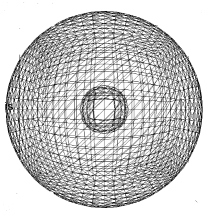
For the computational domain, we take the area between a polyhedral approximation of the sphere of radius , and a polyhedral approximation of a sphere of radius (see Figure 1). The inner sphere represents the obstacle, with an impedance boundary, and the outer sphere is considered far enough away that a Dirichlet (perfect conductor) boundary condition is used. In other words, we prescribe , , and on the outer sphere. The exact solution (taken from [4, Theorem 3.2]) is given as follows:
| (47) | |||||
| (54) | |||||
| (55) |
where for various values of . For the initial conditions, we use piecewise polynomial interpolants of the exponentially-decaying solutions given in equations (47)-(54) at . Further corrections of are needed to make it orthogonal to the gradients of functions in and also to the gradients of the discrete harmonic form. We refer to [1] for details. Finally, for the tests below, we take (). Four different mesh are used in order to test the robustness of the preconditioners with respect to the mesh size and the detailed information about the meshes can be find in Table 1. Numerical experiments are done using a workstation with an 8-Core 3GHz Intel Xeon ‘Sandy Bridge’ CPU and 256 GB of RAM. The software used is a finite-element and multigrid package written by the authors.
| Vertices | Edges | Faces | DoF | |
|---|---|---|---|---|
| Mesh 1 | 602 | 3,210 | 4,812 | 8,624 |
| Mesh 2 | 3,681 | 21,736 | 34,482 | 59,899 |
| Mesh 3 | 27,005 | 171,748 | 282,962 | 481,715 |
| Mesh 4 | 228,412 | 1,525,390 | 2,567,848 | 4,321,650 |
First, we consider the block preconditioners based on well-posedness: the block diagonal preconditioner, (32); the block lower triangular preconditioner, (33); and the block upper triangular preconditioner, (34). The diagonal blocks are solved inexactly by the preconditioned GMRES method with a tolerance of , in order to make sure that the spectral-equivalent properties, (35) and (36), are satisfied. This tolerance is sufficient to meet the conditions in the proof of Theorem 4.5. Since the preconditioners are actually changing at each iteration, we use flexible GMRES (FGMRES) in the implementation with a relative residual stopping criteria of . Table 2 shows the number iterations of the preconditioned FGMRES method with the three different block preconditioners. In these tests, we fix and investigate the robustness of the proposed preconditioners with respect to the time step size, , and mesh size. The iteration counts shown in Table 2 are recorded at the second time step, though the iterations for other time steps are similar. Based on the results, we see that the block preconditioners are effective and robust with respect to these parameters.
(right) Block Upper Triangular, (34). Diagonal blocks are solved inexactly.
| 1 | 2 | 3 | 4 | |
|---|---|---|---|---|
| 21 | 26 | 27 | 28 | |
| 14 | 20 | 25 | 27 | |
| 10 | 14 | 25 | 24 | |
| 7 | 9 | 14 | 20 | |
| 1 | 2 | 3 | 4 |
|---|---|---|---|
| 7 | 8 | 8 | 9 |
| 6 | 7 | 7 | 8 |
| 5 | 5 | 6 | 7 |
| 4 | 5 | 5 | 6 |
| 1 | 2 | 3 | 4 |
|---|---|---|---|
| 7 | 8 | 8 | 9 |
| 6 | 7 | 8 | 8 |
| 5 | 6 | 6 | 8 |
| 5 | 5 | 6 | 6 |
Next, we consider the block preconditioners based on exact block factorization, namely, the block lower triangular preconditioner, , the block upper triangular preconditioner, , and the symmetric preconditioner, , all defined in (42). The diagonal blocks are also solved inexactly by preconditioned GMRES with a relative residual reduction set at . As before, the outer FGMRES iterations are terminated when the value of the norm of the relative residual goes below . Table 3 shows the number of iterations of preconditioned FGMRES with the three different block preconditioners. In these tests, we again fix and see that the block preconditioners based on exact block factorization are effective and robust with respect to and mesh size.
| 1 | 2 | 3 | 4 | |
|---|---|---|---|---|
| 5 | 6 | 6 | 6 | |
| 5 | 5 | 6 | 5 | |
| 5 | 5 | 5 | 6 | |
| 4 | 5 | 5 | 5 | |
| 1 | 2 | 3 | 4 |
|---|---|---|---|
| 6 | 6 | 6 | 7 |
| 5 | 5 | 6 | 7 |
| 5 | 5 | 6 | 6 |
| 5 | 5 | 5 | 6 |
| 1 | 2 | 3 | 4 |
|---|---|---|---|
| 4 | 4 | 4 | 5 |
| 4 | 4 | 4 | 4 |
| 4 | 4 | 4 | 4 |
| 4 | 4 | 4 | 4 |
Finally, we investigate the robustness of the proposed block preconditioners with respect to the physical parameters, and . We fix the mesh size (Mesh 3 is used in all the following tests) and time step size, , and consider jumps in and . The tolerance of the inner GMRES iterations for solving each diagonal block remains for relative residual reduction and the outer FGMRES iterations are terminated when the relative residual has norm smaller than . As before, the iterations count are for the second time step, with other time steps obtaining similar values.
Table 4 reports the number of iterations when there is jump in , but is fixed to be . The jump is chosen so that in the spherical annulus between radius and , as well as between radius and . The jump appears between radius and and ranges from to . The results confirm that the proposed precondtioners are robust with respect to jumps in .
| 28 | 28 | 27 | 25 | 27 | 21 | 16 | |
| 9 | 9 | 8 | 7 | 7 | 9 | 8 | |
| 9 | 9 | 8 | 8 | 7 | 6 | 6 | |
| 7 | 8 | 7 | 6 | 6 | 8 | 8 | |
| 7 | 7 | 6 | 6 | 6 | 5 | 5 | |
| 4 | 4 | 4 | 4 | 4 | 4 | 4 |
Table 5 reports similar results for jumps in , but with is fixed to be . Similarly to the previous case, the jump appears between radius and and ranges from to . Outside this region, . The results show that the proposed precondtioners are also robust with respect to jumps in .
| 17 | 22 | 27 | 25 | 25 | 25 | 25 | |
| 10 | 10 | 9 | 7 | 7 | 7 | 7 | |
| 9 | 9 | 8 | 8 | 8 | 8 | 8 | |
| 9 | 9 | 8 | 6 | 6 | 6 | 6 | |
| 6 | 6 | 6 | 6 | 6 | 6 | 6 | |
| 5 | 5 | 4 | 4 | 4 | 4 | 4 |
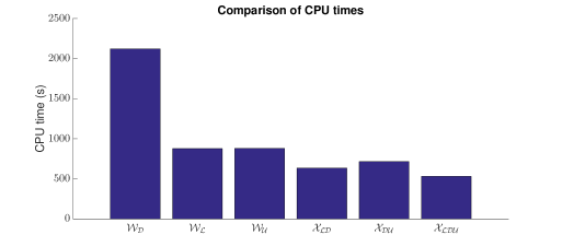
Analyzing the results in Tables 2–5, we see that the block preconditoners based on exact block factorization perform slightly better than the block preconditioners based on well-posedness in terms of iteration count. The dominant cost in computing the action of each of these preconditioners, however, is in approximately solving the diagonal blocks. Since such components are present in all of the preconditioners tested, the overall computational work of applying each of them is similar. Figure 2 confirms this result when comparing the timing to completely solve the system over 20 time steps on the finest grid, Mesh 4, with (again assuming ). Overall, using yields the most efficient results.
6 Conclusions
In [1], it was shown that a structure-preserving discretization of the full time-dependent Maxwell’s equations is capable of resolving the numerical approximation of ADS. Here, we show that the resulting linear systems are also solved efficiently. Block preconditioners for GMRES based on either the well-posedness of the discretization or on a block factorization approach yield linear solvers that are robust with respect to simulation parameters, including time step size and mesh size, as well as the physical parameters of the problem. In the process, we have additionally shown the well-posedness of the structure-preserving discretization and how to preserve the divergence-free constraint for the magnetic field within the linear solver itself.
Such block preconditioners can be applied to other systems, including those discretized with high-order finite elements which are part of a deRham complex. Future work involves extending these results to other applications for which exponentially-decaying solutions exist. By using symplectic time integration and structure-preserving discretizations, we will apply the ideas developed here to build block preconditioners that will efficiently solve for the solutions that preserve important physical properties.
Acknowledgements. Ludmil Zikatanov gratefully acknowledges the support for this work from the Department of Mathematics at Tufts University.
References
- [1] J. H. Adler, V. Petkov, and L. T. Zikatanov. Numerical approximation of asymptotically disappearing solutions of maxwell’s equations. SIAM J. Sci. Comput., 35(5):S386–S401, 2013.
- [2] M. Benzi and G. H. Golub. A preconditioner for generalized saddle point problems. SIAM J. Matrix Anal. Appl., 26(1):20–41, 2005.
- [3] M. Benzi, G. H. Golub, and J. Liesen. Numerical solution of saddle point problems. Acta Numer., 14:1–137, 2005.
- [4] F. Colombini, V. Petkov, and J. Rauch. Incoming and disappearing solutions for Maxwell’s equations. Proc. Amer. Math. Soc., 139(6):2163–2173, 2011.
- [5] F. Colombini, V. Petkov, and J. Rauch. Spectral problems for non-elliptic symmetric systems with dissipative boundary conditions. J. Funct. Anal., 267(6):1637–1661, 2014.
- [6] E. C. Cyr, J. N. Shadid, and R. S. Tuminaro. A new approximate block factorization preconditioner for two-dimensional incompressible (reduced) resistive MHD. SIAM J. Sci. Comput., 35(3):701–730, 2013.
- [7] H. C. Elman, V. E. Howle, J. N. Shadid, R. Shuttleworth, and R. S. Tuminaro. Block preconditioners based on approximate commutators. SIAM J. Sci. Comput., 27(5):1651–1668, 2006.
- [8] H. C. Elman, D. J. Silvester, and A. J. Wathen. Finite elements and fast iterative solvers: with applications in incompressible fluid dynamics. OUP Oxford, 2005.
- [9] K. Feng. On difference schemes and symplectic geometry. In Proceedings of the 1984 Beijing symposium on differential geometry and differential equations, pages 42–58. Science Press, Beijing, 1985.
- [10] K. Feng. Difference schemes for Hamiltonian formalism and symplectic geometry. J. Comput. Math., 4(3):279–289, 1986.
- [11] K. Feng and M. Z. Qin. Symplectic geometric algorithms for Hamiltonian systems. Zhejiang Science and Technology Publishing House, Hangzhou; Springer, Heidelberg, 2010. Translated and revised from the Chinese original, With a foreword by Feng Duan.
- [12] K. Feng, H. M. Wu, and M. Z. Qin. Symplectic difference schemes for linear Hamiltonian canonical systems. J. Comput. Math., 8(4):371–380, 1990.
- [13] R. Hiptmair and J. Xu. Nodal auxiliary space preconditioning in and spaces. SIAM J. Numer. Anal., 45(6):2483–2509, 2007.
- [14] K. Hu, Y. Ma, and J. Xu. Stable finite element methods preserving exactly for MHD models. Submitted to Numerische Mathematik, 2014.
- [15] A. Klawonn. Block-triangular preconditioners for saddle point problems with a penalty term. SIAM Journal on Scientific Computing, 19:172, 1998.
- [16] D. Loghin and A. J. Wathen. Analysis of preconditioners for saddle-point problems. SIAM J. Sci. Comput., 25(6):2029–2049, 2004.
- [17] Y. Ma, K. Hu, X. Hu, and J. Xu. Robust preconditioners for incompressible mhd models. arXiv preprint arXiv:1503.02553, 2015.
- [18] A. Majda. Disappearing solutions for the dissipative wave equation. Indiana Univ. Math. J., 24(12):1119–1133, 1974/75.
- [19] A. Majda. The location of the spectrum for the dissipative acoustic operator. Indiana Univ. Math. J., 25(10):973–987, 1976.
- [20] K. A. Mardal and R. Winther. Uniform preconditioners for the time dependent Stokes problem. Numer. Math., 98(2):305–327, 2004.
- [21] K. A. Mardal and R. Winther. Preconditioning discretizations of systems of partial differential equations. Numer. Linear Algebra Appl., 2010.
- [22] V. Petkov. Scattering theory for hyperbolic operators, volume 21 of Studies in Mathematics and its Applications. North-Holland Publishing Co., Amsterdam, 1989.
- [23] V. Petkov. Scattering problems for symmetric systems with dissipative boundary conditions. In Studies in phase space analysis with applications to PDEs, volume 84 of Progr. Nonlinear Differential Equations Appl., pages 337–353. Birkhäuser/Springer, New York, 2013.
- [24] E. G. Phillips, H. C. Elman, E. C. Cyr, J. N Shadid, and R. P. Pawlowski. A block preconditioner for an exact penalty formulation for stationary mhd. SIAM J. Sci. Comput., 36(6):B930–B951, 2014.
- [25] T. Rusten and R. Winther. A preconditioned iterative method for saddlepoint problems. SIAM J. Matrix Anal. Appl., 13(3):887–904, 1992. Iterative methods in numerical linear algebra (Copper Mountain, CO, 1990).
- [26] J. Schöberl and W. Zulehner. Symmetric indefinite preconditioners for saddle point problems with applications to PDE-constrained optimization problems. SIAM J. Matrix Anal. Appl., 29(3):752—-773, 2007.
- [27] P. S. Vassilevski. Multilevel block factorization preconditioners. Springer, New York, 2008. Matrix-based analysis and algorithms for solving finite element equations.