Algebraic theory of endohedrally confined diatomic molecules: application to H₂@C₆₀

Abstract

A simple and yet powerful approach for modeling the structure of endohedrally confined diatomic molecules is introduced. The theory, based on a $u(4)\oplus u(3)$ dynamical algebra, combines $u(4)$, the vibron model dynamical algebra, with a $u(3)$ dynamical algebra that models a spherically symmetric three dimensional potential. The first algebra encompasses the internal roto-vibrations degrees of freedom of the molecule, while the second takes into account the confined molecule center-of-mass degrees of freedom. A resulting subalgebra chain is connected to the underlying physics and the model is applied to the prototypical case of H₂ caged in a fullerene molecule. The spectrum of the supramolecular complex H₂@C₆₀ is described with a few parameters and predictions for not yet detected levels are made. Our fits suggest that the quantum numbers of a few lines should be reassigned to obtain better agreement with data.

I Introduction

Supramolecular species in which a guest atom or molecule is inserted in the interior of a host molecule (usually fullerenes), are known as endohedral compounds, and form systems that are bound by the pure confinement rather than by intra-molecular forces. The first endohedral compounds obtained consisted of trapped metal atoms Chai et al. (1991) followed by endofullerenes with a trapped molecule Ito et al. (2008). These systems display a full gamut of quantum effects, because the confinement of the molecule results in the splitting of the translational degrees of freedom of the incarcerated molecule center of mass and their coupling with roto-vibrational ones. A fundamental breakthrough that has allowed the application of different spectroscopic tools to molecular endofullerenes has been the achievement of high reaction yields in their synthesis using the so called ”molecular surgery” (See e.g. Refs. Levitt and Horsewill (2013); Komatsu (2013) and references therein). Komatsu and coworkers have presented the synthesis of the endohedral species H₂@C₆₀, that is the subject of the present work Komatsu et al. (2005). Another impressive step forward in this area has been Murata’s group achievement, using similar experimental techniques, of the synthesis of a closed water endofullerene Kurotobi and Murata (2011) and the recent encapsulation of hydrogen fluoride inside C₆₀ Krachmalnicoff et al. (2016).

Significant experimental and theoretical research efforts have been devoted to the elucidation of the spectral properties of H₂@C₆₀ due to the remarkable quantum effects that link roto-vibrational and translational degrees of freedom, coming into play once the diatomic molecule is trapped into the buckyball. In the case of incarcerated H₂, the well known existence of two allotropes of the hydrogen molecule, para-H₂ and ortho-H₂, make this compound a valuable tool for explorations in spin chemistry Turro et al. (2010). These fascinating characteristics of the supramolecular complex H₂@C₆₀ have stimulated remarkable experimental efforts with different techniques Mamone et al. (2011); Levitt and Horsewill (2013), mainly Nuclear Magnetic Resonance (NMR) Komatsu et al. (2005); Carravetta et al. (2007); Turro et al. (2010), InfraRed (IR) Mamone et al. (2009); Ge et al. (2011); Rõõm et al. (2013), and Inelastic Neutron Scattering (INS) Horsewill et al. (2010, 2012, 2013); Xu et al. (2014); Mamone et al. (2016). In particular, an INS spectroscopy selection rule of H₂@C₆₀ has been recently discovered Xu et al. (2014, 2015); Poirier (2015). The search for an adequate description of the structure and the peculiar properties of this endohedral species has provoked intense theoretical efforts Xu et al. (2008a, b, 2011); Xu and Bačić (2011); Xu et al. (2015); Poirier (2015). This system represents an almost ideal testing ground for theories because it couples the simplest diatomic molecule with an almost perfect spherical cage (the icosahedral symmetry can be neglected for most practical purposes). The neutral molecule retains its bound character but, at the same time, it is affected by the presence of the fullerene: its motion is confined and quantized due to the interaction with the cage, a situation that can be fully explored by powerful and simple symmetry-guided models.

Measurements of the IR spectrum of H₂@C₆₀ from low temperatures up to room temperatures have been performed Mamone et al. (2009); Ge et al. (2011); Rõõm et al. (2013). Combining IR spectroscopy data and INS results, the lowest portion of the endohedral compound spectrum has been measured with sufficient detail to allow the experimental underpinning of the differences, shifts and splitting of the levels with respect to the free H₂ counterpart. The spectrum of the confined H₂ molecule has been interpreted in terms of a very accurate, though computationally involved, five dimensional phenomenological model Xu et al. (2008a, b, 2011); Xu and Bačić (2011). While these five dimensional calculations are accurate and can be used to conveniently describe the observations and to make guesses about still unobserved excited states, it is not completely obvious what is the origin of the perturbations in the potential energy terms. For example in Xu et al. (2008b) the authors use Lennard-Jones potentials for each H-C pair in the complex, realizing that the use of an angular momentum quantum number associated with a harmonic motion of the molecule inside the cage is indeed appropriate. This fact supports the convenience of a computationally inexpensive symmetry-based approach like the one we suggest.

We will describe our algebraic approach in Sect. II, discuss the methodology and the fits to a set of experimental lines in Sect. III, and draw conclusions in Sect. IV.

II Algebraic Approach

Stimulated by the success of the existing approach Mamone et al. (2009); Ge et al. (2011), with the aim of obtaining a simple model that encompasses the main physical ingredients for such an enticing system, we propose in the present manuscript an algebraic theory for the quantum modes of a diatomic molecule confined in an isotropic three-dimensional cage. Symmetry considerations constitute the guiding principle that inspires the treatment of the energy terms obtained from a Hamiltonian operator that includes molecular roto-vibrational and center-of-mass modes, and the coupling of these two subsystems. The rotations and vibrations of the diatomic molecule are described within the vibron model Iachello (1981); Iachello and Levine (1994); Frank and Van Isacker (2005), that amounts to a $u(4)$ Lie algebra arising from the bilinear products of scalar $s,s^{\dagger}$ ($\ell=0$) and vector $p_{\mu},p_{\mu}^{\dagger}$ ($\ell=1,\mu=\pm 1,0$) boson operators Iachello (1981). The fullerene cage is modeled as a spherical three dimensional well and can be dealt with a $u(3)$ Lie algebra, arising from a vector boson operator $q_{\mu},q_{\mu}^{\dagger}$ ($\ell=1,\mu=\pm 1,0$) Iachello (2015). Taking this into consideration we invoke an algebraic model based on the direct sum Lie algebra $u_{p}(4)\oplus u_{q}(3)$ to describe the intrinsic modes of excitations of the supramolecular complex H₂@C₆₀, where we use the subindexes $p$ and $q$ to distinguish the two different sets of degrees of freedom. Our symmetry-inspired scheme should be desirable for at least the following peculiar features: (i) it gives a simple framework that singles out what are the linearly independent energy terms and their connection with physical operators; (ii) it gives a natural explanation for the interaction between translational and roto-vibrational degrees of freedom responsible for term energy splittings; (iii) it also gives a natural explanation for the specific radial and angular dependence ($\{R,\Omega,\Omega_{s}\}$ in the notation of Refs. Mamone et al. (2009); Ge et al. (2011)) of the terms that have been found to contribute to the expansion of the coupling potential function; (iv) it treats on an equal footing para- and ortho-H₂ states; (v) there is no need to find separate sets of parameters for each vibrational band, a single fit encompasses all vibrational states simultaneously; and (vi) it is computationally inexpensive: the matrix elements of each operator are known in closed form and the diagonalization can be performed exactly and rapidly. In addition, it yields precise predictions for higher lying modes that, although unseen heretofore, might be investigated in future.

A model that shares a similar algebraic structure, with a dynamical algebra $u(7)\supset u(3)\oplus u(4)$, has been used in the description of hadronic structure in terms of quark building blocks Bijker et al. (1994); Iachello (2015). In that model the $u(7)$ algebra arises from two Jacobi coordinate vectors that describe quarks inside a baryon plus a scalar boson and it is used for the spatial part of the description that must be supplemented by a fermionic part containing the flavor, spin and color degrees of freedom. While the algebraic structure is very similar, clearly the physics behind the model is completely different.

Our model provides a complete mathematical characterization of all possible interactions that comply with the underlying symmetries and therefore naturally gives a hint of the various physical mechanisms that might generate them. We will confine the present discussion to identifying the most important terms and return to the laborious task of a complete classification in a longer paper Pérez-Bernal and Fortunato .

Among the many possible subalgebra chains, we consider the following dynamical symmetry

$$\begin{array}[]{cccccc}u_{p}(4)\oplus u_{q}(3)&\supset&so_{p}(4)\oplus u_{q}(3)\supset&so_{p}(3)\oplus so_{q}(3)&\supset so_{pq}(3)&\supset so_{pq}(2)\\ ~{}N_{p}\hfill N_{q}{}&&~{}\omega{}\hfill&~{}J\hfill L{}&\Lambda&M_{\Lambda}\end{array}~{},$$ (1)

where we have used the $so(4)$ limit of the vibron model Iachello (1981); Iachello and Levine (1994); Frank and Van Isacker (2005); Iachello (2015) and where the second line gives the quantum numbers associated with the Casimir operators of each algebra. With the proviso that $\omega$ is related to the vibrational quantum number $v$ through $v={\textstyle\frac{1}{2}}(N_{p}-\omega)$, the set $(vJN_{q}L\Lambda)$ corresponds to the quantum numbers used so far in theoretical investigations. The basis states can therefore be labeled, very similarly to Refs. Xu et al. (2008a, b); Ge et al. (2011); Xu et al. (2013); Horsewill et al. (2010, 2012); Mamone et al. (2009, 2011), as $|N_{p}vJ;N_{q}L;\Lambda\rangle$.

The quantum numbers follow the well-known branching rules Frank and Van Isacker (2005); Iachello (2015)

$$\omega =N_{p},N_{p}-2,\ldots,1\text{ or }0~{},$$

$$J =0,1,\ldots,\omega~{},$$

$$L =N_{q},N_{q}-2,\ldots,1\text{ or }0~{},$$ (2)

$$\Lambda =|J-L|,|J-L|+1,\ldots,J+L~{}.$$

$$M_{\Lambda} =-\Lambda,-\Lambda+1,\ldots,\Lambda-1,\Lambda~{}.$$

The total Hamiltonian can be written as

$$\hat{H}_{endo}=\hat{H}_{u_{p}(4)}+\hat{H}_{u_{q}(3)}+\hat{H}_{Coupl}~{},$$ (3)

where the first term represents the vibron model Hamiltonian for rotations and vibrations of a diatomic molecule Iachello and Levine (1994), the second is the quantized motion of the molecular center-of-mass inside the three-dimensional spherically-symmetric confining potential, and the last term includes molecule-cage couplings.

The $u(4)$ vibron model Hamiltonian can be modeled as

$$\hat{H}_{u_{p}(4)}=\hat{H}_{so(4)}+\hat{H}_{Dun}~{},$$ (4)

where the first term contains the two-body Casimir operators of the $so(4)$ dynamical symmetry and the second includes two higher-order terms in a Dunham-like expansion Iachello and Levine (1994); Frank and Van Isacker (2005) where the first term represents a centrifugal correction and the second a rotation-vibration coupling.

$$\hat{H}_{so(4)} =E_{0}+\beta\,\hat{C}_{2}[so_{p}(4)]+\gamma\,\hat{C}_{2}[so_{p}(3)]~{},$$ (5)

$$\hat{H}_{Dun} =\gamma_{2}\hat{C}_{2}[so_{p}(3)]^{2}+\kappa\,\hat{C}_{2}[so_{p}(4)]\hat{C}_{2}[so_{p}(3)]~{}.$$ (6)

The Casimir operators in Eqs. (5) and (6) are diagonal in the chosen basis (1)

$$\langle\alpha|\hat{C}_{2}[so_{p}(4)]|\alpha\rangle= \omega(\omega+2)~{},$$

$$\langle\alpha|\hat{C}_{2}[so_{p}(3)]|\alpha\rangle= J(J+1)~{},$$ (7)

$$\langle\alpha|\hat{C}_{2}[so_{p}(4)]\hat{C}_{2}[so_{p}(3)]|\alpha\rangle= \omega(\omega+2)J(J+1)~{},$$

where $|\alpha\rangle=|N_{p}vJ;N_{q}L;\Lambda\rangle$.

The energy formula obtained for $\hat{H}_{u_{p}(4)}$ is

$$E_{u_{p}(4)}= E_{0}+\beta\,\omega(\omega+2)+\gamma\,J(J+1)$$

$$+\gamma_{2}\Bigl{[}J(J+1)\Bigr{]}^{2}+\kappa\,\Bigl{[}\omega(\omega+2)J(J+1)\Bigr{]}~{},$$ (8)

where $\omega=N_{p},N_{p}-2,\ldots,1~{}{\mbox{o}r}~{}0$ or, alternatively, $v=0,1,\ldots,{\textstyle\frac{1}{2}}(N_{p}-1)~{}{\mbox{o}r}~{}{\textstyle\frac{1}{2}}N_{p}$ and $J=0,1,\ldots,\omega$.

The parameters in Eq. (8) are free parameters that can be adjusted to optimize the agreement with experimental data and can be put in direct correspondence with those defined in the approach of Refs. Mamone et al. (2009); Ge et al. (2011)

The center-of-mass degrees of freedom Hamiltonian, within the $u_{q}(3)$ dynamical symmetry, is

$$\hat{H}_{u_{q}(3)}=a\,\hat{C}_{1}[u_{q}(3)]+b\,\hat{C}_{2}[u_{q}(3)]+c\,\hat{C}_{2}[so_{q}(3)]~{},$$ (9)

where the first term is the number of $q$ bosons and would be the only term in case that the confining potential were an isotropic 3D harmonic oscillator, the second term is an anharmonic correction, and the third term is the H₂ center-of-mass centrifugal energy.

Again the Casimir operators are diagonal in the chosen basis

$$\langle\alpha|\hat{C}_{1}[u_{q}(3)]|\alpha\rangle= N_{q}~{},$$

$$\langle\alpha|\hat{C}_{2}[u_{q}(3)]|\alpha\rangle= N_{q}^{2}~{},$$ (10)

$$\langle\alpha|\hat{C}_{2}[so_{q}(3)]|\alpha\rangle= L(L+1)~{},$$

where $|\alpha\rangle=|N_{p}vJ;N_{q}L;\Lambda\rangle$. The free parameters are $a$, $b$, and $c$ and the spectrum associated to the center-of-mass degrees of freedom can be written down in this approach as

$$E_{u_{q}(3)}=a\,N_{q}+b\,N_{q}^{2}+c\,L(L+1)~{},$$ (11)

where $N_{q}$ is the eigenvalue of the number of quanta operator and $L$ is the orbital angular momentum of the whole confined particle (viz. the center of mass of the H₂ molecule) inside the fullerene cage.

II.1 Diatomic Molecule and Spherical Cage Coupling

The guest diatomic molecule and the cage interact through a number of different physical mechanisms that can be traced back to scalar operators built out of the elements of the different algebras. Even at this level, the model is quite rich, therefore one needs to select the most important operators guided by some physical principle and intuition, rather than looking for global fits that would entail too many parameters. We have found that the relevant terms imply Quadrupole-Quadrupole couplings.

The algebraic scheme entails two sets of quadrupole operators, namely $\hat{Q}_{p}=[p^{\dagger}\times\tilde{p}]^{(2)}$, the quadrupole operators of $u_{p}(4)$, and $\hat{Q}_{q}=[q^{\dagger}\times\tilde{q}]^{(2)}$, the quadrupole operators of $u_{q}(3)$. The former describes the intrinsic (non-null if $J\neq 0$) quadrupole of the H₂ molecule, while the latter can be associated with the quadrupole deformation of the probability amplitude of the whole molecule inside the spherical cage. A scalar coupling can be built from these two operators as $[\hat{Q}_{p}^{(2)}\times\hat{Q}_{q}^{(2)}]^{(0)}$, which is the basis for the coupling term in the Hamiltonian (3). In addition, following the spirit of a Dunham expansion, further terms can be considered that lead us to select the following coupling Hamiltonian:

$$\hat{H}_{Coupl}=\vartheta_{pq}[\hat{Q}_{p}^{(2)}\times\hat{Q}_{q}^{(2)}]^{(0)}+\vartheta_{pqw}\left[\hat{C}_{2}[so_{p}(4)][\hat{Q}_{p}^{(2)}\times\hat{Q}_{q}^{(2)}]^{(0)}+[\hat{Q}_{p}^{(2)}\times\hat{Q}_{q}^{(2)}]^{(0)}\hat{C}_{2}[so_{p}(4)]\right]+v_{pq}\hat{C}_{1}[u_{q}(3)]\hat{C}_{2}[so_{p}(4)]~{}.$$ (12)

The parameters $\vartheta_{pq}$, $\vartheta_{pqw}$, and $v_{pq}$ can be used to adjust the interaction strengths. The most important finding about the $[\hat{Q}_{p}^{(2)}\times\hat{Q}_{q}^{(2)}]^{(0)}$ quadrupole-quadrupole interaction is that it lifts the degeneracy of $\Lambda\neq 0$ multiplets, giving the correct and unusual ordering seen in experiments. For example, the triplet of states with $J=1$, $N_{q}=L=2$ has the ordering $\Lambda=2,3,1$ that cannot be due to a scalar coupling of the rotational and translational angular momentum. In fact, once J (that is the rotational angular momentum) and L (the translational angular momentum) are set, a term of the form $\vec{J}\cdot\vec{L}$ always gives a splitting of the levels $\mid J-L\mid<\Lambda<J+L$ that strictly follows an increasing or decreasing ordering depending on the sign of the strength constant.

Following the appendix of Ref. Shalit and Talmi (1963) or Ref. Edmonds (1974), the matrix elements of the scalar coupling of the $\hat{Q}_{p}$ and $\hat{Q}_{q}$ quadrupole operators are

$$\langle N_{p}\omega J;N_{q}L;\Lambda|[\hat{Q}_{p}^{(2)}\times\hat{Q}_{q}^{(2)}]^{(0)}|N_{p}\omega^{\prime}J^{\prime};N^{\prime}_{q}L^{\prime};\Lambda^{\prime}\rangle=(-1)^{L+\Lambda+J^{\prime}}\sqrt{5}\left\{\begin{array}[]{ccc}J&L&\Lambda\\ L^{\prime}&J^{\prime}&2\\ \end{array}\right\}\langle N_{q}L||\hat{Q}_{q}||N^{\prime}_{q}L^{\prime}\rangle\langle\omega J||\hat{Q}_{p}||\omega^{\prime}J^{\prime}\rangle\delta_{\Lambda,\Lambda^{\prime}}~{}~{}.$$ (13)

Once we separate the molecular and cage degrees of freedom, the reduced matrix elements of the molecular ($\hat{Q}_{p}$) and center-of-mass ($\hat{Q}_{q}$) quadrupole degrees of freedom are Frank and Van Isacker (2005)

$$\langle N_{q}L||\hat{Q}_{q}||N_{q}L\rangle= (2N_{q}+3)\sqrt{\frac{L(L+1)(2L+1)}{6(2L-1)(2L+3)}}~{},$$

$$\langle N_{q}L+2||\hat{Q}_{q}||N_{q}L\rangle= \sqrt{\frac{(N_{q}-L)(N_{q}+L+3)(L+1)(L+2)}{(2L+3)}}~{},$$

$$\langle\omega 0||\hat{Q}_{p}||\omega 0\rangle= 0~{},$$

$$\langle\omega J||\hat{Q}_{p}||\omega J\rangle= (N_{p}+2)\left(1+\frac{J(J+1)}{\omega(\omega+2)}\right)\sqrt{\frac{J(J+1)(2J+1)}{6(2J-1)(2J+3)}}~{},$$

$$\langle\omega J+2||\hat{Q}_{p}||\omega J\rangle= (N_{p}+2)\sqrt{\frac{(\omega-J-1)_{2}(\omega+J+2)_{2}(J+1)(J+2)}{4\omega^{2}(\omega+2)^{2}(2J+3)}}~{},$$

$$\langle\omega+2J-2||\hat{Q}_{p}||\omega J\rangle= \sqrt{\frac{(N_{p}-\omega)(N_{p}+\omega+4)(\omega-J+1)_{4}J(J-1)}{16(\omega+1)_{3}(\omega+2)(2J-1)}}~{},$$

$$\langle\omega+2J||\hat{Q}_{p}||\omega J\rangle= \sqrt{\frac{(N_{p}-\omega)(N_{p}+\omega+4)(\omega-J+1)_{2}(\omega+J+2)_{2}J(J+1)(2J+1)}{24(\omega+1)_{3}(\omega+2)(2J-1)(2J+3)}}~{},$$

$$\langle\omega+2J+2||\hat{Q}_{p}||\omega J\rangle= \sqrt{\frac{(N_{p}-\omega)(N_{p}+\omega+4)(\omega+J+2)_{4}(J+1)(J+2)}{16(\omega+1)_{3}(\omega+2)(2J+3)}}~{},$$

where we introduce the Pochhammer symbol $(a)_{b}=a(a+1)\cdots(a+b-1)$.

The matrix elements for the other two operators in the coupling term (12), $\left[\hat{C}_{2}[so_{p}(4)][\hat{Q}_{p}^{(2)}\times\hat{Q}_{q}^{(2)}]^{(0)}+[\hat{Q}_{p}^{(2)}\times\hat{Q}_{q}^{(2)}]^{(0)}\hat{C}_{2}[so_{p}(4)]\right]$ and $\hat{C}_{1}[u_{q}(3)]\hat{C}_{2}[so_{p}(4)]$ are trivially computed using Eqs. (7), (10), and (13).

Another relevant consideration with regard to the quadrupole-quadrupole coupling is the following: if one defines a total quadrupole operator as the sum of the two effects, $\hat{Q}_{T}=\hat{Q}_{p}+\hat{Q}_{q}$ and takes the ratio of the expectation values of this in the first two excited states, namely $|A\rangle=|00111\rangle$ and $|B\rangle=|01001\rangle$, the resulting expression, $\langle Q\rangle_{A}/\langle Q\rangle_{B}=(N_{p}+2+2/N_{p})/3~{},$ depends only on $N_{p}$, the label of the totally symmetric representation of $u_{p}(4)$ that sets the available Hilbert space for the roto-vibrational degrees of freedom, thus giving an alternative to the usual methods of assessing this parameter Iachello and Levine (1994).

III Experimental Data and Fit Results

We have extracted from the literature a total of 71 line positions, compiling a database that includes 55 IR transitions Ge et al. (2011) and 16 INS transitions Horsewill et al. (2012). In these references, lines have been assigned with initial and final quantum numbers on the basis of experimental evidence and theoretical models.

The first step in the fitting procedure has been the assessment of the parameter $N_{p}$. As experimental data for the endohedrally confined species only involve $v=0,1$ H₂ vibrational states, there is not enough information to estimate the $N_{p}$ parameter for the hydrogen molecule. This parameter is usually fixed considering the ratio between first and second order parameters in the Dunham expansion for the molecule under study Iachello and Levine (1994). Therefore, we devised an alternative way to assess this parameter, using the roto-vibrational spectroscopy of the free H₂ molecule making use of free H₂ vibrational data and explored the $N_{p}$ dependence of the fit to the experimental energy terms beneath $10000$ cm^-1 with a $so(4)$ dynamical symmetry Hamiltonian

$$\hat{H}_{so(4)}= \beta\,\hat{C}_{2}[so(4)]+\gamma\,\hat{C}_{2}[so(3)]$$ (14)

$$+\gamma_{2}\hat{C}_{2}[so(3)]^{2}+\kappa\,\hat{C}_{2}[so(3)]\hat{C}_{2}[so(4)]~{}.$$

The reason for setting an energy threshold is that the inclusion of highly-excited energy levels, close to the molecular dissociation limit, implies the necessity of including continuum effects and resonances that are out of the scope of the vibron model, based on a $u(4)$ compact lie algebra Iachello (1981); Iachello and Levine (1982); Kim et al. (1986). The resulting root mean square (rms) deviation for a fit to a total of 31 roto-vibrational experimental term energies from Refs. Dabrowski (1984); Stanke et al. (2008); Salumbides et al. (2011) is depicted as a function of $N_{p}$ in Fig. 1, where it is clear that the best fit is obtained for $N_{p}=34$ and the resulting parameters can be found in Tab. 1.

Table 1: Parameters of Hamiltonian (14) optimized to reproduce experimental term energies of the free H₂ molecule under $10000\;\text{cm}^{-1}$ with $N_{p}=34$ and $rms$ of the fit. Parameters are given in cm^-1 units. The fit to 31 experimental energy levels has an $rms=4.0\;\text{cm}^{-1}$.

$\beta$	$\gamma$	$\gamma_{2}$	$\kappa$
$1041.54(6)$	$32.80(7)$	$-0.036215(7)$	$0.72423(20)$

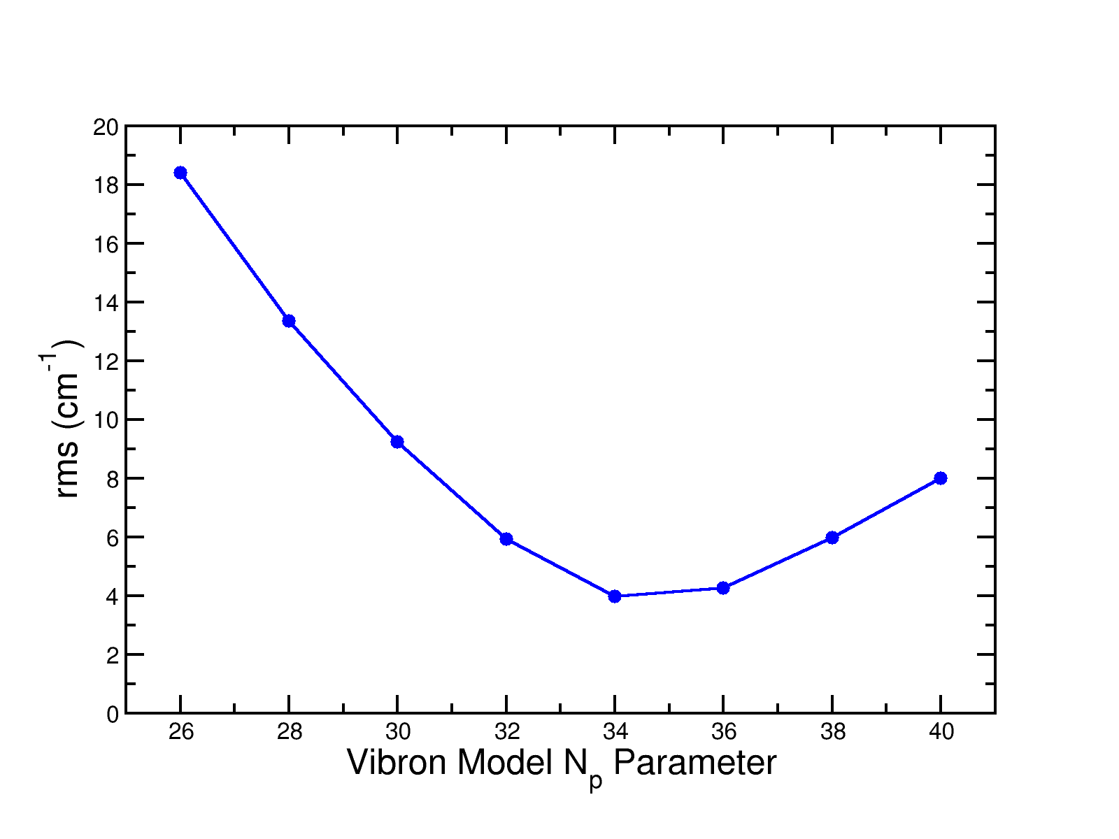
Figure 1: (Color online) Root mean square deviation (rms) for fits to free H₂ roto-vibrational experimental term energies under a threshold value of $10000\;\text{cm}^{-1}$ with Hamiltonian (14) as a function of the number of vibrons parameter $N_{p}$.

With the value of $N_{p}$ set to 34, we can return to the caged system. A Python code has been developed to calculate the eigenvalues and eigenstates of the total Hamiltonian $\hat{H}_{endo}$ that encompasses the molecular roto-vibrational degrees of freedom (4), the incarcerated center-of mass degrees of freedom (9), and the coupling between them (12), and to compute the free parameter values that minimize the difference between calculated results and experimental line positions from Refs. Ge et al. (2011); Horsewill et al. (2012). The code makes use of Sympy SymPy Development Team (2016) and LMFIT Newville et al. (2014) packages and is available under request.

In a preliminary set of calculations we have made several fits to the full data set and to different subsets, obtaining a good overall description. We have found that, leaving aside a constant energy shift, a minimal Hamiltonian that complies with all symmetry requirements and provides results that agree with experimental data, has seven parameters: $\{\beta,\gamma,\kappa,a,b,c,\vartheta_{pq}\}$. The first three from Eqs. (5) and (6), the second three from Eq. (9), plus the low order quadrupole coupling in Eq. (12). The fits with this set are denoted as $F_{0}$.

A finer fit, denoted as $F_{1}$, can be obtained with three more parameters, up to a total of ten free parameters. The three added parameters are $\gamma_{2}$ from Eq. (6), and the coupling parameters $\vartheta_{pqw}$ and $v_{pq}$ of Eq. (12) associated with operators $\left[\hat{C}_{2}[so_{p}(4)][\hat{Q}_{p}^{(2)}\times\hat{Q}_{q}^{(2)}]^{(0)}+[\hat{Q}_{p}^{(2)}\times\hat{Q}_{q}^{(2)}]^{(0)}\hat{C}_{2}[so_{p}(4)]\right]$ and $\hat{C}_{1}[u_{q}(3)]\hat{C}_{2}[so_{p}(4)]$, respectively.

Table 2: Reassigned experimental transitions. Experimental states are given with the quantum numbers $vJN_{q}L\Lambda$. Line positions are given in cm^-1 units.

Old ass.		New ass.
Initial	Final	Initial	Final	Exp.	Ref.
$00200$	$01111$	$00200$	$01110$	$-85.5$	Horsewill et al. (2012)
$01221$	$11311$	$01334$	$11443$	$4294.8$	Ge et al. (2011)
$00200$	$10311$	$01334$	$11445$	$4294.8$	Ge et al. (2011)
$01334$	$11444$	$01221$	$11311$	$4300.0$	Ge et al. (2011)
$01334$	$11445$	$01332$	$12312$	$4316.4$	Ge et al. (2011)

Preliminary calculations gave a satisfactory agreement with the experimental line positions, though some levels had a residual value much larger than expected from the overall fit agreement. This has suggested us to consider a tentative reassignment of a set of five transitions showing unusually large deviations, as indicated in Tab. 2. With this reassignment the quality of the fit has largely improved. The convenience of this reassignment in the framework of this model can be seen in Fig. 2 where the residuals for fits $F_{0}$ and $F_{1}$ are plot as a function of the line position energy. The outcome for the original level assignment is shown in the upper panels, while the residuals with the new level assignment are depicted in the lower panels. The achieved improvement in the fit is remarkable though a deeper analysis is on the way to confirm these assignments and the findings will be published in a forthcoming paper Pérez-Bernal and Fortunato . In the following we refer to the set of experimental states with the five mentioned reassignments.

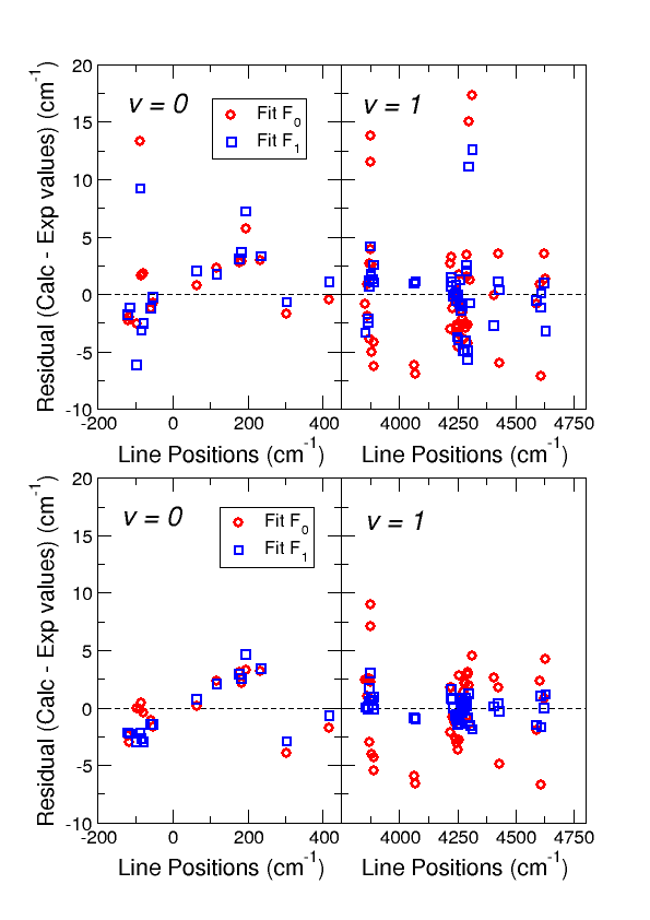
Figure 2: Color online. Residuals of the $F_{0}$ and $F_{1}$ fits (see text) with the original assignments (upper panels) and including the changes suggested in Tab. 2 (lower panels).

The final $F_{0}$ and $F_{1}$ parameters, with root mean square $rms=3.1\;\text{cm}^{-1}$ and $1.7\;\text{cm}^{-1}$, respectively, are given in Tab. 3. The full list of residuals (experimental value minus calculated value) for both fits, plotted in Fig. 2 are given in Tab. 4 together with the experimental line positions and initial and final state assignments.

Table 3: $F_{0}$ (Minimal) and $F_{1}$ (Finer) fits parameter values. In both cases $N_{p}=34$. Hamiltonian parameters and $rms$ are expressed in cm^-1 units.

$\hat{H}_{u_{p}(4)}$	$\beta$	$\gamma$	$\kappa$	$\gamma_{2}$
$F_{0}$	$-1083.23(18)$	$58.09(17)$	$0.88(4)$	–
$F_{1}$	$-1081.72(15)$	$58.28(20)$	$0.810(25)$	$-0.032(15)$
$\hat{H}_{u_{q}(3)}$	$a$	$b$	$c$
$F_{0}$	$178.3(8)$	$9.6(3)$	$-3.26(15)$
$F_{1}$	$179.0(4)$	$8.46(17)$	$-3.18(8)$
$\hat{H}_{Coupl}$	$\vartheta_{pq}$	$\vartheta_{pqw}$	$v_{pq}$
$F_{0}$	$0.94(7)$	–	–
$F_{1}$	$0.86(5)$	$-0.014(7)$	$-1.02(8)$
$rms$	$F_{0}$	$3.1$	$F_{1}$	$1.7$

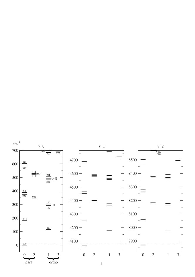
Figure 3: Theoretical roto-vibrational spectrum of H${}_{2}@$C₆₀. The three cuts show the energy levels in a 700 cm^-1 wide energy window just above the three lowest vibrational excitations $v=0,1$, and $2$. States are further divided into para (left) and ortho (right) states and are labeled by $J$ on the horizontal axis and $N_{q}L\Lambda$ on each state. These quantum numbers are repeated with the same order in each panel, except where noted.

Table 4: Residuals for fits $F_{0}$ and $F_{1}$. Initial and final states are denoted by the quantum numbers of basis (1), $vJN_{q}L\Lambda$. Experimental states are extracted from Refs. Ge et al. (2011); Horsewill et al. (2012) and reassigned transitions (see Tab. I) are highlighted in red. Both experimental line positions and residual values are expressed in cm^-1.

Initial	Final	Exp.	Calc. $F_{0}$	Calc. $F_{1}$	Initial	Final	Exp.	Calc. $F_{0}$	Calc. $F_{1}$
0 1 0 0 1	0 0 0 0 0	-118.6	-2.42	-2.16	0 1 0 0 1	1 1 1 1 1	4244.4	-2.76	-0.96
0 1 1 1 1	0 0 1 1 1	-113.7	-3.00	-2.27	0 2 1 1 2	1 2 2 2 3	4250.7	-0.65	-1.12
0 0 2 0 0	0 1 1 1 2	-95.7	-0.06	-3.00	0 1 0 0 1	1 1 1 1 2	4250.7	-3.14	-1.48
0 0 2 0 0	0 1 1 1 0	-85.5	-0.17	-2.19	0 0 0 0 0	1 0 1 1 1	4255.6	-3.649	-1.45
0 0 2 2 2	0 1 1 1 1	-82.7	0.44	-2.67	0 1 1 1 2	1 1 2 2 2	4255.6	-0.84	-0.82
0 0 2 2 2	0 1 1 1 2	-76.9	-0.44	-2.97	0 1 0 0 1	1 1 1 1 0	4261.3	-2.85	-1.43
0 2 0 0 2	0 1 1 1 1	-57.7	-1.09	-1.46	0 2 1 1 1	1 2 2 2 0	4261.3	2.77	0.83
0 2 0 0 2	0 1 1 1 2	-51.6	-1.66	-1.47	0 1 1 1 2	1 1 2 2 3	4267.1	0.64	0.43
0 1 0 0 1	0 0 1 1 1	65.2	0.15	0.73	0 1 1 1 1	1 1 2 2 1	4272.1	-1.05	-0.46
0 0 0 0 0	0 1 0 0 1	118.5	2.32	2.06	0 0 1 1 1	1 0 2 2 2	4272.1	0.25	0.72
0 1 0 0 1	0 1 1 1 1	178.8	3.05	2.91	0 1 2 2 2	1 1 3 3 3	4277.1	1.37	0.46
0 1 0 0 1	0 1 1 1 2	184.5	2.07	2.51	0 1 2 2 3	1 1 3 3 4	4281.2	2.12	0.05
0 1 0 0 1	0 1 1 1 0	196.0	3.26	4.61	0 0 2 2 2	1 0 3 3 3	4286.5	2.06	0.81
0 1 0 0 1	0 2 0 0 2	235.5	3.13	3.38	0 1 1 1 2	1 1 2 0 1	4290.2	0.62	0.55
0 0 0 0 0	0 1 1 1 0	304.9	-4.02	-2.92	0 0 1 1 1	1 0 2 0 0	4290.2	-0.79	0.14
0 1 0 0 1	0 2 1 1 1	417.8	-1.84	-0.71	0 1 3 3 4	1 1 4 4 3	4294.8	2.82	-0.93
0 1 2 0 1	1 1 1 1 2	3855.6	2.37	0.01	0 1 3 3 4	1 1 4 4 5	4294.8	3.10	-0.83
0 0 2 0 0	1 0 1 1 1	3866.0	1.0	0.08	0 1 2 2 1	1 1 3 1 1	4300.0	1.91	1.19
0 1 2 0 1	1 1 1 1 0	3866.0	2.45	-0.14	0 1 2 2 2	1 1 3 1 1	4306.7	-1.424	-1.570
0 2 1 1 3	1 2 0 0 2	3872.2	-3.04	0.59	0 1 3 3 2	1 2 3 1 2	4316.4	4.45	-1.90
0 1 2 2 1	1 1 1 1 1	3872.2	2.53	1.68	0 1 2 0 1	1 3 1 1 2	4407.4	2.63	0.11
0 1 3 3 3	1 1 2 2 2	3876.0	8.92	3.02	0 1 2 2 3	1 3 1 1 4	4426.8	1.77	0.39
0 0 3 3 3	1 0 2 2 2	3878.6	7.04	0.67	0 1 1 1 2	1 3 0 0 3	4431.9	-4.94	-0.30
0 1 2 2 3	1 1 1 1 2	3878.6	2.25	0.96	0 0 0 0 0	1 2 1 1 1	4592.0	-2.02	-1.53
0 0 2 2 2	1 0 1 1 1	3884.9	0.72	0.20	0 0 1 1 1	1 2 2 2 1	4608.9	2.25	1.02
0 1 1 1 2	1 1 0 0 1	3884.9	-4.08	0.62	0 1 0 0 1	1 3 0 0 3	4612.5	-6.77	-1.69
0 1 1 1 1	1 1 0 0 1	3891.3	-4.36	0.92	0 0 1 1 1	1 2 2 0 2	4624.3	0.76	-0.06
0 0 1 1 1	1 0 0 0 0	3891.3	-5.49	-0.16	0 0 2 2 2	1 2 3 3 1	4630.0	4.24	1.14
0 1 0 0 1	1 1 0 0 1	4065.4	-6.01	-0.86	0 1 0 0 1	1 3 1 1 2	4802.6	-2.77	-1.28
0 0 0 0 0	1 0 0 0 0	4071.4	-6.62	-0.96	0 1 1 1 2	1 3 2 2 2	4814.8	0.13	-0.17
0 3 0 0 3	1 3 1 1 4	4223.3	1.70	0.76	0 1 1 1 1	1 3 2 2 2	4821.6	0.26	0.53
0 0 1 1 1	1 2 0 0 2	4223.3	-2.20	1.57	0 1 1 1 1	1 3 2 2 1	4829.7	1.29	1.40
0 3 0 0 3	1 3 1 1 2	4226.2	1.74	0.73	0 1 1 1 2	1 3 2 0 3	4836.2	1.68	1.74
0 2 0 0 2	1 2 1 1 2	4233.1	-0.82	-0.04	0 1 2 2 2	1 3 3 3 1	4846.4	1.83	0.35
0 2 0 0 2	1 2 1 1 3	4239.8	-1.34	-0.72	0 1 2 2 1	1 3 3 1 2	4864.5	-0.96	-2.24
0 2 0 0 2	1 2 1 1 1	4244.4	-1.07	-0.56

The quality and robustness of our calculations allows us to estimate the energies of levels not yet accessed experimentally. We have included in Fig. 3 the calculated $v=0,1$, and $2$ levels, the latter not yet measured. One can notice that, with growing $v$, the higher the $J$ the bigger the negative energy shift of corresponding states. An extensive table with all calculated levels for $v=0,1,2$ vibrational quanta with $N_{q}\leq 4$ and $\Lambda\leq 5$ can be found in the Supplemental Material section. In addition to the term energy, expressed in cm^-1 units, we also indicate in the table the probability of the largest component (squared coefficient) of the corresponding eigenstate expressed in basis (1).

IV Summary and Conclusions

In summary, we have introduced a $u(4)\oplus u(3)$ algebraic scheme that combines the vibron model description of a diatomic molecule roto-vibrational structure with an algebraic description of the motion of the molecule center-of-mass inside an isotropic cage. This model is mathematically rich and has a large number of possible terms that can be attributed to different physical mechanisms. We have presented here a discussion of a few selected physical mechanisms that, in spite of the model’s simplicity, give insight into the spectroscopic properties of diatomic endohedrally confined molecules. We have then applied the symmetry-guided scheme to a database of experimental lines, finding a very good overall agreement to the experimental line positions and finding that the fits improve considerably upon reassigning the quantum numbers of a small subset of energy levels.

The next step is the inclusion of transition intensities in the model and the enrichment of the approach, that could take place in one of two possible venues, either by defining an embedding $u_{pq}(7)\supset u_{p}(4)\oplus u_{q}(3)$ dynamical algebra or by a dynamical algebra $u_{p}(4)\oplus u_{q}(4)$ with results that will be published soon Pérez-Bernal and Fortunato . Another venue for future research is the inclusion in the algebraic model of the cage icosahedral symmetry effect on the spectrum, that has recently been investigated Poirier (2015); Mamone et al. (2016).