On Leader Green Election

Abstract

We investigate the number of survivors in the Leader Green Election (LGE) algorithm introduced by P. Jacquet, D. Milioris and P. Mühlethaler in 2013. Our method is based on the Rice method and gives quite precise formulas. We derive upper bounds on the number of survivors in this algorithm and we propose a proper use of LGE.

Finally, we discuss one property of a general urns and balls problem and show a lower bound for a required number of rounds for a large class of distributed leader election protocols.

1 Introduction

In Jacquet et al. (2013) Philippe Jacquet, Dimitris Milioris and Paul Mühlethaler introduced a novel energy efficient broadcast leader election algorithm, which they called, in accordance with the popular fashion in those years, a Leader Green Election (LGE). This algorithm was also presented by P. Jacquet at the conference AofA’13.

We will use the same model as in Jacquet et al. (2013), namely we assume that the communication medium is of the broadcast type and is prone to collisions. We also assume that the time is slotted. Each slot can be empty (the slot does not contain any burst), collision (the slot contains at least two burst) or successful (the slot contains a single burst).

During the investigation of efficiency of LGE algorithm we found a connection of the leader election problem with some properties of the general ”‘urns and balls”’ model. This connection is discussed in Section 3.

1.1 Short Description of LGE

We will give a short description of a slightly simplified version of the LGE algorithm (for example, authors of Jacquet et al. (2013) consider an arbitrary base of numeral systems, but we restrict our considerations only to base $3$, since some additional arguments, not presented in this paper, show that base-3 is an optimal choice for our purposes).

We assume that the broadcast medium has $N$ connected users (assume $N\approx 10^{6}$) and that the number of contenders $n$ is always smaller or equal to $N$. We fix a number $p\in(0,1)$ and we assume that p is not close to one (e.g. $p=0.01$). We also fix a number $L=\mathrm{O}\left(\log\log N\right)$.

Each contender $\omega$ selects independently a random number $g_{\omega}$ according to the geometric distribution with parameter $p$ (see next section for details). If $g_{\omega}\geq 3^{L+1}$ then we put $g_{\omega}=0$. The number $g_{\omega}$ is written

$$g_{\omega}=\sum_{k=0}^{L}b_{k}\cdot 3^{k}~{},$$ (1)

where $b_{k}\in\{0,1,2\}$. We fix a function $f:\{0,1,2\}\to\{0,1\}^{2}$ by $f(0)=00$, $f(1)=01$ and $f(2)=10$, and define the transmission key $K_{\omega}$ for a contender $\omega$ as the concatenation

$$K_{\omega}=f(b_{L})||f(b_{L-1})||\ldots||f(b_{1})||f(b_{0})~{}.$$

Notice that lenght($K_{\omega}$) = $\mathrm{O}\left(\log\log N\right)$. This key $K_{\omega}$ is used in the following algorithm played in discrete rounds:

1:  candidate = true

2:  for i=1 to lenght($K_{\omega}$) do

3:     if $K_{\omega}(i)$ = 1 then

4:        send a beep

5:     else

6:        listen

7:        if you hear a beep then

8:           candidate = false

9:           exit loop

10:        end if

11:     end if

12:  end for

The survivors of this algorithm are those contenders which at the end have the variable ”candidate” set to true. In Jacquet et al. (2013) authors propose to repeat this algorithm several times in order to reduce the number of survivors to 1. However we propose in this paper an another approach: we propose to use this algorithm only once (in order to reduce number of survivors to a small number) and then to use other leader election algorithm for final selection a leader.

1.2 Mathematical Background

The core of LGE algorithm is based on properties of extremal statistics of random variables with geometric distributions. Let us recall that a random variable $X$ has a geometric distribution with parameter $p\in[0,1]$ ($X\sim\mathrm{Geo}(p)$) if $P[X=k]=(1-p)^{k-1}p$ for $k\geq 1$. In the first part of LGE, each user chooses independently a random variable with geometric distribution with a fixed parameter $p$. The winners of this part of LGE are those users who select a maximal number.

Definition 1

A random variable $M$ has distribution $\mathrm{MGeo}(n,p)$ if there are independent random variables $X_{1},\ldots,X_{n}$ with distribution $\mathrm{Geo}(p)$ such that

$$M=\max\{X_{1},\ldots,X_{n}\}~{}.$$

It is well known (see e.g. Szpankowski and Rego (1990), Cichoń and Klonowski (2013)) that if $M\sim\mathrm{MGeo}(n,p)$ then $\mathbf{E}\left[M\right]$ = $\frac{1}{2}+\frac{\mathrm{H_{n}}}{\ln\frac{1}{1-p}}+P(n)+\mathrm{O}\left(\frac{1}{n}\right)$, where $P(n)$ is a periodic function with small amplitude and $\mathrm{H_{n}}$ is the $n^{\mathrm{th}}$ harmonic number. Let us recall that $\mathrm{H_{n}}=\ln n+\gamma+\mathrm{O}\left(\frac{1}{n}\right)$, where $\gamma=0.557\ldots$ is the Euler constant.

The distribution $\mathrm{MGeo}(n,p)$ controls the number of time slots used in LGE algorithm. More precisely, the LGE algorithm requires some upper approximation on the variable with the $\mathrm{MGeo}(n,p)$ distribution. The next Lemma gives some upper bound for it.

Lemma 1

Let $M\sim\mathrm{MGeo}(n,p)$, $C>0$ and $Q=\frac{1}{1-p}$. Then

$$\Pr[M>C\frac{\ln n}{\ln Q}]\leq\frac{1}{n^{C-1}}~{}.$$

Proof 1.1.

Let $q=1-p$. Let us recall that if $X\sim\mathrm{Geo}(p)$ and $k$ is an integer then $\Pr[X>k]=q^{k}$. Therefore $\Pr[M>k]\leq nq^{k}$, hence $\Pr\left[M>C\frac{\ln n}{\ln Q}\right]\leq nq^{C\frac{\ln n}{\ln Q}}=\frac{1}{n^{C-1}}$.

We introduce the next distribution which models the number of survivors in LGE algorithm.

Definition 1.2.

A random variable $W$ has distribution $\mathrm{WMGeo}(n,p)$ if there are independent random variables $X_{1},\ldots,X_{n}$ with distribution $\mathrm{Geo}(p)$ such that

$$W=\mathrm{card}\left(\{k:X_{k}=\max\{X_{1},\ldots,X_{n}\}\}\right)~{}.$$

2 Probabilistic Propeties of LGE

The formal analysis of LGE algorithm in Jacquet et al. (2013) is based on the Mellin transform. In this section, we use an approach based on Rice’s method (see e.g. Knuth (1998) and Flajolet and Sedgewick (1995)). We shall derive formulas for expected number of survivors and probabilities for the number of survivors. By $W_{n,p}$ we denote a random variable with $\mathrm{WMGeo}(n,p)$ distribution.

Theorem 2.3.

Let $n\geq 2$, $p\in(0,1)$ and $q=1-p$. Let $W_{n,p}\sim\mathrm{WMGeo}(n,p)$ and $a\geq 1$. Then

$$\Pr[W_{n,p}=a]=\binom{n}{a}p^{a}\sum_{b=0}^{n-a}\binom{n-a}{b}\frac{(-1)^{b}}{1-q^{a+b}}$$

and

$$\mathbf{E}\left[W_{n,p}\right]=\frac{np}{q}\sum_{b=0}^{n-1}\binom{n-1}{b}\frac{(-1)^{b}}{1-q^{b+1}}~{}.$$

Proof 2.4.

Let us fix $n\geq 2$, $p\in(0,1)$ and $q=1-p$. Let $X_{1},\ldots,X_{n}$ be independent random variables with distribution $\mathrm{Geo}(p)$ and let

$$A_{n;k,a}=(\max\{X_{1},\ldots,X_{n}\}=k)\land(\mathrm{card}\left(\{i:X_{i}=k\}=a\right))~{}.$$

Then $[W_{n,p}=a]=\bigcup_{k\geq 1}A_{n;k,a}$ and $\Pr[A_{n;k,a}]=\binom{n}{a}(q^{k-1}p)^{a}(1-q^{k-1})^{n-a}$. Therefore,

$$\Pr[W_{n}=a]=\sum_{k\geq 1}\binom{n}{a}(q^{k-1}p)^{a}(1-q^{k-1})^{n-a}=$$

$$\binom{n}{a}p^{a}\sum_{k\geq 0}q^{ka}(1-q^{k})^{n-a}=\binom{n}{a}p^{a}\sum_{k\geq 0}\sum_{b=0}^{n-a}\binom{n-a}{b}(-1)^{b}q^{kb}q^{ka}=$$

$$\binom{n}{a}p^{a}\sum_{b=0}^{n-a}\binom{n-a}{b}(-1)^{b}\sum_{k\geq 0}q^{k(b+a)}=\binom{n}{a}p^{a}\sum_{b=0}^{n-a}\binom{n-a}{b}\frac{(-1)^{b}}{1-q^{a+b}}~{},$$

so the first part of the Theorem is proved. Next we have

$$\sum_{a=1}^{n}a\Pr[A_{n;k,a}]=n\sum_{a=1}^{n}\binom{n-1}{a-1}(q^{k-1}p)^{a}(1-q^{k-1})^{n-a}=$$

$$nq^{k-1}p\sum_{a=1}^{n}\binom{n-1}{a-1}(q^{k-1}p)^{a-1}(1-q^{k-1})^{(n-1)-(a-1)}=$$

$$nq^{k-1}p\sum_{b=0}^{n-1}\binom{n-1}{b}(q^{k-1}p)^{b}(1-q^{k-1})^{(n-1)-b}=$$

$$nq^{k-1}p(q^{k-1}p+1-q^{k-1})^{n-1}=nq^{k-1}p(1-q^{k})^{n-1}~{}.$$

Therefore, for fixed $n$, we have

$$\sum_{k\geq 1}\sum_{a=1}^{n}a\Pr[A_{k,a}]=\sum_{k\geq 1}npq^{k-1}\sum_{b=0}^{n-1}\binom{n-1}{b}(-1)^{b}q^{kb}=$$

$$np\sum_{b=0}^{n-1}\binom{n-1}{b}(-1)^{b}\sum_{k\geq 1}q^{k-1}q^{kb}=\frac{np}{q}\sum_{b=0}^{n-1}\binom{n-1}{b}(-1)^{b}\sum_{k\geq 1}q^{k}q^{kb}=$$

$$\frac{np}{q}\sum_{b=0}^{n-1}\binom{n-1}{b}(-1)^{b}\sum_{k\geq 1}q^{k(b+1)}=\frac{np}{q}\sum_{b=0}^{n-1}\binom{n-1}{b}(-1)^{b}q^{b+1}\sum_{k\geq 0}(q^{b+1})^{k}=$$

$$\frac{np}{q}\sum_{b=0}^{n-1}\binom{n-1}{b}\frac{(-1)^{b}q^{b+1}}{1-q^{b+1}}~{}.$$

Since we assumed that $n\geq 2$, we have

$$\frac{np}{q}\sum_{b=0}^{n-1}\binom{n-1}{b}\frac{(-1)^{b}q^{b+1}}{1-q^{b+1}}=\frac{np}{q}\sum_{b=0}^{n-1}\binom{n-1}{b}(-1)^{b}\frac{(q^{b+1}-1)+1}{1-q^{b+1}}=$$

$$-\frac{np}{q}\sum_{b=0}^{n-1}\binom{n-1}{b}(-1)^{b}+\frac{np}{q}\sum_{b=0}^{n-1}\binom{n-1}{b}(-1)^{b}\frac{1}{1-q^{b+1}}=$$

$$-\frac{np}{q}(-1+1)^{n-1}+\frac{np}{q}\sum_{b=0}^{n-1}\binom{n-1}{b}\frac{(-1)^{b}}{1-q^{b+1}}=\frac{np}{q}\sum_{b=0}^{n-1}\binom{n-1}{b}\frac{(-1)^{b}}{1-q^{b+1}}~{}.$$

From Theorem 2.3 we obtain the following equality $\Pr[W_{n,p}=1]$ = $np\sum_{b=0}^{n-1}\binom{n-1}{b}\frac{(-1)^{b}}{1-q^{1+b}}$. Therefore, we have the following nice equality

$$\mathbf{E}\left[W_{n,p}\right]=\frac{1}{1-p}\Pr[W_{n,p}=1]~{}.$$

Remark Quite recently we learned that Theorem 2.3 and part of results from the next subsection has been proved in Kirschenhofer and Prodinger (1996). Due to the completeness of arguments we decided to leave the proof in this paper. Our new contribution in this section is the Theorem 2.12.

2.1 Approximations

Let us fix the number $p\in(0,1)$ and let $q=1-p$. Let $f_{a}(z)=\frac{1}{1-q^{a+z}}$. We shall consider complex variable functions $f_{a}$ for such indexes $a$ which are integers such that $a\geq 1$. Notice that the function $f_{a}$ has singularities at points from the set $\{\zeta_{a,k}:k\in\mathbb{Z}\}$, where $\zeta_{a,k}=-a+\frac{2k\pi\mathbf{i}}{\ln(q)}$. The function $f_{a}$ is periodic with period $2\pi\mathbf{i}/\ln(q)$, has single poles at points $\zeta_{a,k}$ and

$$\mathrm{Res}(f_{a}(z):z=\zeta_{a,k})=\frac{-1}{\ln q}~{}.$$

It is easy to check that $\lim_{x\to\infty}|f_{a}(x+\mathbf{i}y)|=1$ and $\lim_{x\to-\infty}|f_{a}(x+\mathbf{i}y)|=0$ for each fixed $y\in\mathbb{R}$.

Let $K_{n}(s)=\frac{n!}{s(s-1)\cdots(s-n)}$. Notice that if $n\geq 1$ then $|K_{n}(s)|=\mathrm{O}\left(\frac{1}{|s|^{2}}\right)$ as $|s|$ grows to infinity. Also notice that if $a>0$ is an integer, then $K_{n}(-a)=(-1)^{n+1}\frac{1}{a}\binom{n}{a}^{-1}$. Notice also that the sets of singularity points of functions $f_{a}$ and $K_{n}$ are disjoint. This fact greatly simplifies the analysis of the singular points of the product of these functions

Lemma 2.5.

If $m\geq 1$, $a\geq 1$ and $q\in(0,1)$ then

$$\sum_{b=0}^{m}\binom{m}{b}\frac{(-1)^{b}}{1-q^{a+b}}=(-1)^{m}\frac{1}{\ln q}\sum_{k\in\mathbb{Z}}K_{m}(\zeta_{a,k})~{}.$$

Proof 2.6.

Rice’s integrals summation method (see Knuth (1998)) is based on the formula

$$\sum_{b=0}^{m}\binom{m}{b}(-1)^{b}g(b)=\frac{(-1)^{m}}{2\pi i}\oint_{\mathcal{C}}g(s)K_{m}(s)ds~{},$$

where $g$ is analytic in a domain containing $[0,+\infty)$ and $\mathcal{C}$ is a positively oriented closed curve that lies in the domain of analyticity of $g$ and encircles the real interval $[0,m]$.

We use Rice’ formula for functions $f_{a}$. Notice that

$$\frac{1}{2\pi i}\oint_{\mathcal{C}}f_{a}(s)K_{m}(s)ds=\sum_{k=0}^{m}\mathrm{Res}(f_{a}(z)K_{m}(z):z=k)~{}.$$

Let $C_{k}$ be the positively oriented square with corners at points $\pm\eta_{q,k}\pm\eta_{q,k}\mathbf{i}$, where $\eta_{q,k}=(2k+1)\pi/\ln q$. We consider such $k$ that $|\eta_{q,k}|>m$. For such $k$ the interval $[0,m]$ lies inside the square $C_{k}$. The mentioned before Lemma 2.5 properties of the function $f_{a}$ (periodicity and boundedness on horizontal lines not crossing singular points) and the kernel function $K_{m}$ imply that

$$\lim_{k\to\infty}\oint_{C_{k}}f_{a}(s)K_{m}(s)ds=0~{},$$

from which we deduce that

$$\sum_{k\in\mathbb{Z}}\mathrm{Res}(f_{a}(z)K_{m}(z):z=\zeta_{a,k})+\sum_{k=0}^{m}\mathrm{Res}(f_{a}(z)K_{m}(z):z=k)=0~{}.$$

Therefore,

$$\sum_{b=0}^{m}\binom{m}{b}\frac{(-1)^{b}}{1-q^{a+b}}=(-1)^{m+1}\sum_{k\in\mathbb{Z}}\mathrm{Res}(f_{a}(z)K_{m}(z):z=\zeta_{a,k})=$$

$$(-1)^{m+1}\sum_{k\in\mathbb{Z}}\mathrm{Res}(f_{a}(z):z=\zeta_{a,k})K_{m}(\zeta_{a,k})=(-1)^{m+1}\sum_{k\in\mathbb{Z}}\frac{-1}{\ln q}K_{m}(\zeta_{a,k}).$$

Lemma 2.7.

Suppose that $a>0$ is an integer and that $b\in\mathbb{C}$. Then

$$K_{m}(-a+b)=\frac{(-1)^{m+1}}{a\binom{a+m}{a}}\cdot\frac{1}{\prod_{j=a}^{m+a}(1-\frac{b}{j})}~{}.$$

Proof 2.8.

Directly from the definition of the kernel function $K_{m}$ we have

$$K_{m}(-a+b)=m!\prod_{j=0}^{m}\frac{1}{-a+b-j}=(-1)^{m+1}m!\prod_{j=0}^{m}\frac{1}{a+j-b}=$$

$$(-1)^{m+1}m!\prod_{j=a}^{m+a}\frac{1}{j-b}=(-1)^{m+1}m!\prod_{j=a}^{m+a}\frac{1}{j(1-\frac{b}{j})}=$$

$$(-1)^{m+1}m!\frac{(a-1)!}{(m+a)!}\prod_{j=a}^{m+a}\frac{1}{(1-\frac{b}{j})}~{}.$$

The next Lemma follows directly from Theorem 2.3, Lemmas 2.5 and 2.7:

Lemma 2.9.

If $n>a$ then

$$\Pr[W_{n,p}=a]=\frac{p^{a}}{a\ln\frac{1}{q}}\left(1+\sum_{k\in\mathbb{Z}\setminus\{0\}}\frac{1}{\prod_{j=a}^{n}(1-\frac{2k\pi\mathbf{i}/\ln q}{j})}\right)~{},$$

where $q=1-p$.

Theorem 2.10.

If $0<a<n$ then $\Pr[W_{n,p}=a]=\frac{p^{a}}{a\ln(Q)}+r_{n}$, where $|r_{n}|<\frac{(a+1)^{2}}{12a}p^{a}\ln(Q)$, where $Q=\frac{1}{1-p}$.

Proof 2.11.

Let $\eta_{k}=\frac{2\pi k\mathbf{i}}{\ln q}$, where $q=1-p$. Notice that

$$\left|\prod_{j=a}^{n}(1-\frac{\eta_{k}}{j})\right|^{2}=\prod_{j=a}^{n}\left(1+\frac{|\eta_{k}|^{2}}{j^{2}}\right)\geq\prod_{j=a}^{a+1}\left(1+\frac{|\eta_{k}|^{2}}{j^{2}}\right)\geq\left(1+\frac{|\eta_{k}|^{2}}{(a+1)^{2}}\right)^{2}~{}.$$

Therefore,

$$\left|\sum_{k\in\mathbb{Z}\setminus\{0\}}\prod_{j=a}^{n}\frac{1}{1-\frac{\eta_{k}}{j}}\right|\leq 2\sum_{k=1}^{\infty}\frac{1}{1+\frac{|\eta_{k}|^{2}}{(a+1)^{2}}}\leq 2(a+1)^{2}\sum_{k=1}^{\infty}\frac{1}{|\eta_{k}|^{2}}=$$

$$\frac{(a+1)^{2}(\ln q)^{2}}{2\pi^{2}}\sum_{k=1}^{\infty}\frac{1}{k^{2}}=\frac{(a+1)^{2}(\ln q)^{2}}{12}~{},$$

so the conclusion follows from Lemma 2.9.

Let us fix $p\in(0,1)$, let $Q=\frac{1}{1-p}$. We put

$$\phi_{p}(a)=\frac{p^{a}}{a\ln{Q}}+\frac{(a+1)^{2}}{12a}p^{a}\ln{Q}.$$

Notice that $\Pr[W_{n,p}=a]\leq\phi_{p}(a)$.

Theorem 2.12.

$\Pr[W_{n}\geq k]<\frac{\phi(k)}{1-2p}$

Proof 2.13.

It can be observed that $\frac{\phi_{p}(a+1)}{\phi_{p}(a)}<2p$. Therefore,

$$\Pr[W_{n}\geq k]=\sum_{a=k}^{n}\Pr[W_{n}=a]<\sum_{a=k}^{\infty}\phi(a)<\frac{\phi(k)}{1-2p}~{}.$$

2.2 Discussion

Let us observe that formulas from Theorem 2.10 do not depend on the number $n$. However, small fluctuations (which are very interesting from theoretical point of view) are hidden inside the error term, which can be observed on the Fig. 1.

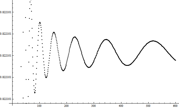
Figure 1: Plot of $\Pr[W_{n,\frac{1}{3}}=1]$ for $n=1,\ldots,600$.

This practical independence of the number $n$ of nodes on the number of survivors is very interesting. However, the number $n$ has an influence on the required number of rounds in LGE. This number may be controlled by Lemma 1: from this lemma we deduce that if $X\sim\mathrm{MGeo}(n,p)$ then $\Pr[X>(\ln 10^{20}+\ln n)/\ln(Q)]<10^{-20}$ (where $Q=1/(1-p)$), and hence from a practical point of view it is negligible. This implies that (see Jacquet et al. (2013) for details) the LGE algorithm should run $2\cdot\left\lceil\log_{3}\left(\frac{1}{\ln(Q)}(\ln n+\ln(10^{20})\right)\right\rceil$ rounds in order to ensure that its probabilistic properties are controlled by the distribution $\mathrm{WGeo}$ with probability at least $1-10^{-20}$.

From Theorem 2.10 we deduce that $\Pr[W_{n,p}=1]=1-\frac{p}{2}+\mathrm{O}\left(p^{2}\right)$ and $\Pr[W_{n,p}=2]=\frac{p}{2}+\mathrm{O}\left(p^{2}\right)$. From these formulas we deduce that the probability of failure of one phase of LGE is quite large. However, notice that from Theorem 2.12 we get $\Pr[W_{n,0.01}>10]\approx 1.006\cdot 10^{-19}$. Therefore, the LGE algorithm may be used for quick reduction of potential leaders to a small subgroup. We see that if we use this algorithm with parameter $p=\frac{1}{100}$, then with probability at least $1-10^{-19}$, the number of survivors will be less or equal $10$. The survivors may then take part in another algorithm (e.g. in an algorithm based on paper Prodinger (1993) or in algorithm based on paper Janson and Szpankowski (1997), Louchard and Prodinger (2009)), which deals better with small sets of nodes, in order to select a leader with high and controllable probability.

3 Lower Bound

In the previous section we recalled that the LGE algorithm should use $\mathrm{O}\left(\ln\ln(n)\right)$ rounds in order to achieve high effectiveness. In this section we prove a general result confirming that this bound is near to an optimal. We use a method applied by D. E. Willard in Willard (1986) for an analysis of resolution protocols in a multiple access channel.

Let us consider a system $(U_{i})_{i=1,\ldots,L}$ of $L$ urns and let us fix a number $n$. We consider a process of throwing an arbitrary number $Q\in\{2,\ldots,n\}$ of balls into these urns. We assume that all balls are thrown independently and that the probability that the ball is thrown into $i$th urn is equal $p_{i}$. This process is fully described by the vector $\vec{p}$ of probabilities from the simplex $\Sigma_{L}=\{(p_{1},\ldots,p_{L})\in[0,1]^{L}:p_{1}+\ldots+p_{L}=1\}$ and the number $Q$ of balls.

The most broadly studied model of urns and balls is the uniform case, i.e. the case when $\vec{p}=(\frac{1}{L},\ldots,\frac{1}{L})$. However, in several papers (see e.g. Flajolet et al. (1992), Boneh and Hofri (1997)) one can find some results for the general case. In this section we are interested in the existence of at least one singleton, i.e. in the existence of an urn $U_{i}$ with precisely one ball. The problem of estimation of the number of singletons was quite recently analyzed in Penrose (2009).

Let $S_{\vec{p},Q}$ denote the event ”there exists at least one urn with a single ball” and let $S_{\vec{p},Q,i}$ denote the event ”there is exactly one ball in $i$th urn”. Then, $\Pr[S_{\vec{p},Q,i}]=Qp_{i}(1-p_{i})^{Q-1}$ and $S_{\vec{p},Q}=\bigcup_{i=1}^{L}S_{\vec{p},Q,i}$, therefore, $\Pr[S_{\vec{p},Q}]\leq Q\sum_{i=1}^{L}p_{i}(1-p_{i})^{Q-1}$.

Let us assume that the number $Q$ of balls is unknown but it is bounded by a number $n$. We are going to show that if the number $n$ is sufficiently large compared to $L$, then there is no $\vec{p}\in\Sigma_{L}$ which will guarantee the existence of singleton with a high probability for arbitrary $Q$ from $\{2,\ldots,n\}$. More precisely, let

$$\mathrm{MSP}\left(L,n\right)=\max_{\vec{p}\in\Sigma_{L}}\min_{2\leq Q\leq n}\Pr[S_{\vec{p},Q}]~{}.$$

(term MSP is an abbreviation of ”Maximal Success Probability”).

Theorem 3.14.

For arbitrary $L\geq 1$ and $n\geq 2$, we have

$$\mathrm{MSP}\left(L,n\right)<\frac{L-1}{\mathrm{H_{n}}-1}~{}.$$

Proof 3.15.

Let us observe that if $\vec{p}\in\Sigma_{L}$ is such that for some $i$ we have $p_{i}=1$ and $Q\geq 2$, then $\Pr[S_{\vec{p},Q}]=0$, so $\min_{2\leq Q\leq n}\Pr[S_{\vec{p},Q}]=0$. Hence, we may consider only such $\vec{p}\in\Sigma_{L}$ that $p_{i}<1$ for each $i=1,\ldots,L$.

Let us fix the number $L$ of urns and let us consider the following function (this is the trick which we borrow from Willard (1986)):

$$f(\vec{p})=\sum_{Q=2}^{n}\frac{\Pr[S_{\vec{p},Q}]}{Q}~{}.$$

Then we have

$$f(\vec{p})\leq\sum_{Q=2}^{n}\sum_{i=1}^{L}\frac{\Pr[S_{\vec{p},Q,i}]}{Q}=\sum_{Q=2}^{n}\sum_{i=1}^{L}p_{i}(1-p_{i})^{Q-1}\leq\sum_{i=1}^{L}\sum_{Q=2}^{\infty}p_{i}(1-p_{i})^{Q-1}=$$

$$\sum_{i=1}^{L}p_{i}(1-p_{i})\frac{1}{1-(1-p_{i})}=\sum_{i=1}^{L}(1-p_{i})=L-\sum_{i=1}^{L}p_{i}=L-1~{}.$$

On the other side, let $p^{*}=\min\{\Pr[S_{\vec{p},Q}]:2\leq Q\leq n\}$. Then we have

$$f(\vec{p})\geq\sum_{Q=2}^{n}\frac{p^{*}}{Q}=p^{*}\sum_{Q=2}^{n}\frac{1}{Q}=p^{*}(\mathrm{H_{n}}-1)~{}.$$

Therefore, we have

$$p^{*}(\mathrm{H_{n}}-1)\leq f(\vec{p})<L-1~{}.$$

Hence, if we take $Q^{*}$ such that $\Pr[S_{\vec{p},Q^{*}}]=p*$, then

$$\Pr[S_{\vec{p},Q^{*}}]<\frac{L-1}{\mathrm{H_{n}}-1}~{},$$

so

$$\min_{2\leq Q\leq n}\Pr[S_{\vec{p},Q}]<\frac{L-1}{\mathrm{H_{n}}-1}$$

for arbitrary $\vec{p}\in\Sigma_{n}$.

Corollary 3.16.

If $1\leq L\leq\frac{1}{2}\ln n+\frac{1+\gamma}{2}$ then $\mathrm{MSP}\left(L,n\right)<\frac{1}{2}$.

Corollary 3.17.

If $n\geq\exp(2L-(1+\gamma))$ then $\mathrm{MSP}\left(L,n\right)<\frac{1}{2}$.

Proof 3.18.

Both proofs follow directly from Theorem 3.14 and the inequality $\mathrm{H_{n}}\geq\ln(n)+\gamma$.

3.1 Application to Leader Election Problem

Let us consider any oblivious leader election algorithm in which at the beginning each station selects randomly and independently a sequence of bits of length $M$, and later this station use the sequence in the algorithm in a deterministic way. Let $n$ denote the upper bound on the number of stations taking part in this algorithm and let $b_{i}$ denote the sequence of bits chosen by the $i$th station. Observe that if for each $i$ there is $j\neq i$ such that $b_{i}=b_{j}$, then the algorithm must fail. Hence, success is possible only if there is a singleton in choices made from the space $\{0,1\}^{M}$ of all possible sequences of bits. When we use Corollary 3.16 with $L=2^{M}$, then we deduce that if $M\leq\log_{2}\left(\frac{1}{2}\ln n+\frac{1+\gamma}{2}\right)$ then the probability that the considered algorithm chooses a leader is less than $\frac{1}{2}$. We may say that $\log_{2}(\frac{1}{2}\ln n)$ random bits are too few for distinguishing an arbitrary collection of $\leq n$ objects with a high probability.

References

• Boneh and Hofri (1997) A. Boneh and M. Hofri. The coupon-collector problem revisited—a survey of engineering problems and computational methods. Stochastic Models, 13(1):39–66, 1997.
• Cichoń and Klonowski (2013) J. Cichoń and M. Klonowski. On flooding in the presence of random faults. Fundam. Inform., 123(3):273–287, 2013.
• Flajolet and Sedgewick (1995) P. Flajolet and R. Sedgewick. Mellin transforms and asymptotics: Finite differences and Rice’s integrals. Theor. Comput. Sci., 144(1,2):101–124, 1995. URL http://dblp.uni-trier.de/db/journals/tcs/tcs144.html#FlajoletS95.
• Flajolet et al. (1992) P. Flajolet, D. Gardy, and L. Thimonier. Birthday paradox, Coupon collectors, Caching algorithms and Self-organizing search. Discrete Appl. Math., 39(3):207–229, Nov. 1992. ISSN 0166-218X. 10.1016/0166-218X(92)90177-C. URL http://dx.doi.org/10.1016/0166-218X(92)90177-C.
• Jacquet et al. (2013) P. Jacquet, D. Milioris, and P. Mühlethaler. A novel energy efficient broadcast leader election. In MASCOTS, pages 495–504. IEEE, 2013.
• Janson and Szpankowski (1997) S. Janson and W. Szpankowski. Analysis of an asymmetric leader election algorithm. Electr. J. Comb., 4(1), 1997. URL http://www.combinatorics.org/Volume_4/Abstracts/v4i1r17.html.
• Kirschenhofer and Prodinger (1996) P. Kirschenhofer and H. Prodinger. The number of winners in a discrete geometrically distributed sample. Ann. Appl. Probab., 6(2):687–694, 05 1996. 10.1214/aoap/1034968150. URL http://dx.doi.org/10.1214/aoap/1034968150.
• Knuth (1998) D. E. Knuth. The Art of Computer Programming, Volume 3: (2Nd Ed.) Sorting and Searching. Addison Wesley Longman Publishing Co., Inc., Redwood City, CA, USA, 1998. ISBN 0-201-89685-0.
• Louchard and Prodinger (2009) G. Louchard and H. Prodinger. The asymmetric leader election algorithm: Another approach. Annals of Combinatorics, 12:449–478, 2009.
• Penrose (2009) M. Penrose. Normal approximation for isolated balls in an urn allocation model. Electron. J. Probab., 14:no. 74, 2155–2181, 2009. ISSN 1083-6489. 10.1214/EJP.v14-699. URL http://ejp.ejpecp.org/article/view/699.
• Prodinger (1993) H. Prodinger. How to select a loser. Discrete Mathematics, 120(1-3):149–159, 1993. 10.1016/0012-365X(93)90572-B. URL http://dx.doi.org/10.1016/0012-365X(93)90572-B.
• Szpankowski and Rego (1990) W. Szpankowski and V. Rego. Yet another application of a binomial recurrence. Order statistics. Computing, 43(4):401–410, Feb. 1990. ISSN 0010-485X. 10.1007/BF02241658. URL http://dx.doi.org/10.1007/BF02241658.
• Willard (1986) D. E. Willard. Log-logarithmic selection resolution protocols in a multiple access channel. SIAM J. Comput., 15(2):468–477, May 1986. ISSN 0097-5397. 10.1137/0215032. URL http://dx.doi.org/10.1137/0215032.