MIMO Precoding for Networked Control Systems with Energy Harvesting Sensors

Abstract

In this paper, we consider a MIMO networked control system with an energy harvesting sensor, where an unstable MIMO dynamic system is connected to a controller via a MIMO fading channel. We focus on the energy harvesting and MIMO precoding design at the sensor so as to stabilize the unstable MIMO dynamic plant subject to the energy availability constraint at the sensor. Using the Lyapunov optimization approach, we propose a closed-form dynamic energy harvesting and dynamic MIMO precoding solution, which has an event-driven control structure. Furthermore, the MIMO precoding solution is shown to have an eigenvalue water-filling structure, where the water level depends on the state estimation covariance, energy queue and the channel state, and the sea bed level depends on the state estimation covariance. The proposed scheme is also compared with various baselines and we show that significant performance gains can be achieved.

I Introduction

Networked control systems (NCSs) have become quite popular recently due to their growing applications in industrial automation, smart transportation, remote robotic control, etc.. A typical NCS consists of a multiple-input multiple-output (MIMO) dynamic plant , a multiple antenna wireless sensor and a controller. These are connected over a communication network and form a closed-loop control, as illustrated in Figure 1. Compared to traditional wireless sensors that are powered by a non-rechargeable battery, we consider an energy harvesting sensor, which is equipped with an energy harvesting device (e.g., a solar panel or a micro wind turbine) so that the sensor can harvest energy from the surrounding environment. Such NCSs with energy harvesting sensors have many advantages. For example, they do not require the replacement of batteries (for traditional sensors) and the maintenance process is simplified for NCSs in dangerous environments (e.g., chemical plants).

For an NCS, a potentially unstable plant is stabilized using a sensor to measure the state and feeds back to a controller, which in turn drives a stabilizing control signal to the plant. Unlike conventional feedback control design where the feedback path is assumed to be perfect, the sensor in the NCS observes the plant state and transmits the observation to a remote controller over a wireless MIMO fading channel. The performance of the NCS is closely related to the communication resource control at the energy harvesting sensor over the MIMO wireless channel. For an energy harvesting sensor, the communication resource is related to the energy available in the battery. Due to the random nature of the renewable energy source, it is difficult to predict the future evolution of the energy arrivals, and hence there is a tradeoff of using the available energy to support the current transmission and saving the energy for future good transmission opportunities.

In fact, NCS is a multidisciplinary subject involving both control theory and communication theory. The main objective of the control theory is to control the plant such that its state evolves in a desired manner. The plant is usually modeled as a linear dynamic system which is described by a set of first order coupled linear difference equations representing the evolution of the state variables. The representation of a plant with linear system provides a convenient and compact way to model and analyze the plant. Stability is an important characteristic of control system. When a plant is unstable, the state of the plant may be unbounded even though the input to the plant is bounded. General uncertainties and external disturbances may cause the dynamic plant to be unstable and this may incur costly physical damage. For instance, an unstable aircraft may crash and an unstable chemical plant may explode. Therefore, it is extremely important stabilize the unstable dynamic plant.

The theory of Lyapunov drift has a long history in the field of stochastic control to analyze the system stability in the field of control and communications. The authors of [2] first applied the Lyapunov drift theory to develop a general algorithm which stabilizes a multi-hop packet radio network. The negative Lyapunov drift terms play a central role when applying the Lyapunov drift theory to analyze the stability of dynamic systems. Intuitively, the negative Lyapunov drift is a stabilizing force that pulls the system state back to the equilibrium point. In [3], it is shown that negative Lyapunov drift ensures network stability because whenever the data queue length vector leaves a certain bounded region, the negative drift eventually drives it back to that region. In [4], the negative Lyapunov drift is utilized to analyze the stability of Markov chains.

From the communication side, it is important to understand how to optimize the communication resources (such as MIMO precoding) targeted for control applications. In particular, MIMO precoder optimization has been well studied in wireless communications. A MIMO precoder is essentially a multimode beamformer which splits the transmit signal into spatial eigenbeams and assigns higher power along the beams when the channel is strong [5]. In [6, 7], the authors obtain the MIMO linear precoding solution to minimize the MMSE [6] or maximize the SINR [7] of the MIMO wireless systems. However, these precoding solutions are not tailored for NCS applications because the optimization objectives (MMSE or SINR) are merely physical layer metrics in wireless communications, which may not be directly related to the performance metric of the NCS applications (such as stability of the plant or plant state estimation errors). Another related development in wireless communications is the device-to-device (D2D) or machine-to-machine (M2M) communications where a communication device can communicate and exchange information with a peer device autonomously. One important application of D2D or M2M systems (in addition to delivering content) is to support real-time industrial control where the devices may act as sensors and/or actuators. As such, these new application scenarios embrace both wireless communications and control in the context of networked control systems. In this paper, we are interested in studying the design of the MIMO precoder in the communication subsystem to support NCS applications.

Note that communication resource allocation for an NCS with an energy harvesting sensor is quite challenging. This is because such a problem embraces the information theory (to model the physical layer over the wireless channels), the queuing theory (to model the energy queue dynamics) and the control theory (to model the plant dynamics under imperfect state feedback control). There are some works on the dynamic resource control design for NCSs with an energy harvesting sensor. In [8], the authors study the mean square average state estimation error minimization under renewable energy constraints. To obtain the optimal communication power control policies, the associated stochastic optimization problems are solved using the numerical value iteration algorithm, which induces huge complexity, and suffers from slow convergence and lack of insights [9]. In this paper, we propose a low-complexity closed-form dynamic MIMO precoding solution at the sensor powered by renewable energy to stabilize the unstable MIMO dynamic plant. The following summarizes the key contributions in the paper.

• Direct Analog State Transmission with Peak Power Constraint: Unlike existing approaches in NCS [10, 11, 12] where the plant state is first quantized and transmitted over a simplified digital channel, we propose a novel analog state transmission where the sensor simply transmits a spatially rotated state measurement (rotated by the MIMO precoder) to the remote controller without quantization or coding. The consideration of renewable energy source also poses a unique challenge. For instance, the sensor needs to equip with a limiter, which is a non-linear module to attenuate peaks of signals to satisfy the peak power constraint . Such design will simplify the datapath design of the sensor and the remote controller and directly take advantage of the MIMO communication channels.

• Closed-form Dynamic Event-Triggered MIMO Precoder Policy: Event-triggered sensor control has been proposed in various existing NCS applications [12, 13]. However, the existing solutions either has no closed-form triggering solution [12, 13] or the solution is not truly dynamic [12]. In addition, in all these existing solutions, there is no consideration of the multi-antenna MIMO communication channels. In this paper, we derive a closed-form fully dynamic solution which adapts to the complete system state (MIMO channel state for transmission opportunity, sensor energy state for energy availability and plant state estimation error for the urgency of the state transmission). These agile adaptivity are very important for superb performance in the NCS application.

• Closed-form Performance Characterizations: In this paper, we also derive closed-form requirement of the renewable energy arrival rate and the battery capacity requirement to attain stability of the MIMO NCS. Such results give important guideline for the dimensioning of the resource needed at the sensor. Furthermore, we have derived closed form MSE and study how the performance depends on key system parameters. Such closed-form derivation is challenging due to the dynamic MIMO precoding policy as well as the coupled system state evolutions where the dynamic evolution of the three system states (the energy state, the plant state and the MIMO channel state) are tightly coupled together in a very complicated manner.

Notations: Uppercase and lowercase boldface denote matrices and vectors, respectively. The operators $(\cdot)^{T}$, $(\cdot)^{\dagger}$, $(\cdot)^{H}$, $\mathrm{Tr\left(\cdot\right)}$, $|\cdot|$, $\mathrm{Re}\left\{\cdot\right\}$, $\mathbf{1}{\{\cdot\}}$ are the transpose, element-wise conjugate, conjugate transpose, trace, cardinality, real part, and indicator function, respectively; $||\mathbf{A}||$ and $||\mathbf{a}||$ denote spectrum norm of matrix $\mathbf{A}$ and Euclidean norm of vector $\mathbf{a}$, respectively; and $\text{diag}(\textbf{a})$ means diagonal matrix with diagonal elements being a; $\mathbf{A}_{ij}$ denotes the element in the $i$-th row and $j$-th column of matrix $\mathbf{A}$; $\mu_{i}\left(\mathbf{A}\right)$ denotes the $i$-th largest eigenvalue of matrix $\mathbf{A}$. $\mathbb{R}^{m\times n}$ ($\mathbb{C}^{m\times n}$) represents the set of $m\times n$ dimensional real (complex) matrices.

II System Model

In this section, we introduce the model of the MIMO NCS with an energy harvesting sensor, plant dynamics, MIMO channel model, energy queue model, as well as the information structures at the sensor and the controller.

II-A MIMO Networked Control System with an Energy Harvesting Sensor

Figure 1 shows a typical networked control system (NCS) with a MIMO plant (potentially unstable), a multi-antenna sensor (with $N_{s}$ transmit antennas) with energy harvesting capability and a multi-antenna remote controller (with $N_{c}$ receive antennas). The sensor and the controller are geographically separated and connected through a wireless MIMO fading channel. We consider a time-slotted system with slot duration $\tau$. The sensor has perfect observation of the MIMO plant state $\mathbf{x}\left(n\right)$ at every time slot. Due to the consideration of renewable energy source at the sensor, the observed plant state $\mathbf{x}\left(n\right)$ is passed through an energy limiter before the transmission so as to satisfy an instantaneous peak power constraint determined by the instantaneous available energy. The output of the limiter is $\mathbf{q}\left(n\right)$. Unlike conventional digital approaches in NCS, we consider direct analog transmission of the measured system state at the sensor. Specifically, the analog state measurement is spatially rotated by a MIMO precoder $\mathbf{F}(n)$ and transmits to the remote controller over the multi-antenna wireless fading channel. We assume the perfect channel state information can be obtained at the sensor by causal signaling feedback from the controller as illustrated in Figure 1. The received signal at the controller is $\mathbf{y}(n)$, which is passed to the state estimator to obtain a state estimate $\hat{\mathbf{x}}\left(n\right)$. Based on $\hat{\mathbf{x}}\left(n\right)$, the remote controller further generates the control action $\mathbf{u}\left(n\right)$. The controller is physically attached to the actuator of the plant so that the control action $\mathbf{u}\left(n\right)$ generated at the controller can be applied to the plant directly. The actuator, which is co-located with the plant, then applies $\mathbf{u}\left(n\right)$ for plant actuation. The goal of the MIMO NCS is to stabilize the potentially unstable MIMO plant with limited wireless communication resources.

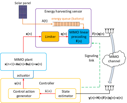
Figure 1: A typical architecture of a MIMO NCS with an energy harvesting sensor. In this paper, we focus on the dynamic design of the limiter and MIMO precoder.

II-B Stochastic Dynamic MIMO Plant Model

We consider a discrete-time stochastic MIMO plant system with state dynamics: $\mathbf{x}\left(n+1\right)=\mathbf{A}\mathbf{x}\left(n\right)+\mathbf{B}\mathbf{u}\left(n\right)+\mathbf{w}\left(n\right)$, $\ n\geq 0$, $\mathbf{x}\left(0\right)=\mathbf{x}_{0}$, where $\mathbf{x}\left(n\right)\in\mathbb{R}^{K\times 1}$ is the plant state process, $\mathbf{u}\left(n\right)\in\mathbb{R}^{D\times 1}$ is the plant control action, $\mathbf{A}\in\mathbb{R}^{K\times K}$, $\mathbf{B}\in\mathbb{R}^{K\times D}$, and $\mathbf{w}\left(n\right)\in\mathbb{R}^{K\times 1}$ is the plant noise. We assume the plant noise $\mathbf{w}\left(n\right)\in\mathbb{R}^{K\times 1}$ is zero mean with covariance $\mathbb{E}\left[\mathbf{w}\left(i\right)\left(\mathbf{w}\left(j\right)\right)^{T}\right]=\delta_{i,j}\mathbf{W}$ for $\forall i,j$, where $\delta_{i,j}=0$ if $i\neq j$ and $\delta_{i,j}=1$ otherwise. We assume that the plant noise covariance is finite . The MIMO plant system $(\mathbf{A},\mathbf{B})$ is assumed to be controllable with $\mathbf{A}$ containing possibly unstable eigenvalues.

II-C MIMO Wireless Channel Model

We model the wireless communication channel between the multi-antenna sensor and the controller as a wireless MIMO fading channel. Using multiple-antenna techniques, the $N_{s}$-antenna sensor can deliver $K$ parallel data streams to the $N_{c}$-antenna controller through spatial multiplexing. We assume $K\leq\mathrm{min}\left\{N_{s},N_{c}\right\}$. At the $n$-th time slot, the received signal $\mathbf{y}\left(n\right)$ at the controller is given by

$$\mathbf{y}\left(n\right)=\mathbf{H}\left(n\right)\mathbf{F}\left(n\right)\mathbf{q}\left(n\right)+\mathbf{z}\left(n\right),$$ (1)

where $\mathbf{H}\left(n\right)\in\mathbb{C}^{N_{c}\times N_{s}}$ is the MIMO channel fading matrix, $\mathbf{F}\left(n\right)\in\mathbb{C}^{N_{s}\times K}$ is the MIMO precoding matrix, $\mathbf{q}(n)$ is the output of the energy limiter, and $\mathbf{z}\left(n\right)\sim\mathcal{CN}\left(0,\mathbf{I}_{N_{s}}\right)$ is the additive complex Gaussian noise. We have the following assumption on $\mathbf{H}\left(n\right):$

Assumption 1

(MIMO Wireless Channel Model) The random MIMO channel realization $\mathbf{H}\left(n\right)$ remains constant within each time slot. Furthermore, $\mathbf{H}(n)$ is i.i.d. across different time slots according to some general distribution.

II-D Energy Harvesting and Energy Queue Model at the Sensor

We assume the sensor is solely powered by renewable energy sources (such as a solar panel). Due to the random nature of the energy source, a battery or ultra-capacitor is needed to store the harvested energy at the sensor. Let $\alpha\left(n\right)$ be the amount of harvestable energy at the sensor at time slot $n$. We have the following assumption on harvestable energy process $\alpha\left(n\right)$.

Assumption 2

(Renewable Energy Model) The harvestable energy $\alpha\left(n\right)$ is i.i.d. across different time slots according to some distribution.

The sensor has an energy storage (or battery) so let $E\left(n\right)$ be the amount of energy left in the storage device at time $n$. We assume that the sensor is causal in the sense that new energy arrivals are observed after the control actions are performed at each time slot. Hence, the energy queue dynamics at the sensor is given by

$$E\left(n+1\right) =\mathrm{min}\left\{\left[E\left(n\right)-\|\mathbf{F}\left(n\right)\mathbf{q}\left(n\right)\|^{2}\tau\right]^{+}+\alpha\left(n\right),\theta\right\},$$ (2)

where $\left[x\right]^{+}=\mathrm{max}\left\{x,0\right\}$, $\|\mathbf{F}\left(n\right)\mathbf{q}\left(n\right)\|^{2}\tau$ measures the energy consumed at time slot $n$ for delivering $\mathbf{q}\left(n\right)$ using precoding action $\mathbf{F}\left(n\right)$ over the MIMO wireless fading channel, and $\theta$ is the sensor battery capacity. Furthermore, at any time slot $n$, the precoding control action must satisfy the following energy availability constraint:

$$\|\mathbf{F}\left(n\right)\mathbf{q}\left(n\right)\|^{2}\tau\leq E\left(n\right).$$ (3)

Challenge 1: Energy Availability Constraint and Saturation.

The energy availability constraint (3) means that the energy consumption at each time slot cannot exceed the current available energy in the energy buffer at the sensor. Such a constraint greatly complicates the design of the dynamic MIMO precoder at the sensor. At any time slot, the dynamic MIMO precoder has to strike a balance between how much energy to consume, the good transmission opportunities induced by the fading channel and the $urgency$ induced by the state estimation errors at the controller. Furthermore, there is an effective peak transmission power constraint at the sensor at each time slot. In order to satisfy this constraint, the sensor needs to be equipped with a limiter. Since the input process $\mathbf{x}\left(n\right)$ is non-stationary with unbounded support, there is non-zero chance that the input $\mathbf{x}\left(n\right)$ exceeds the limiter range, causing saturation. This causes non-linearity in the feedback loop and substantially complicates the optimization problem. In the next section, we introduce the design of the limiter, and we will elaborate how we tackle the issue of saturation in Section III-B.

II-E Energy Limiter at the Sensor

An energy limiter is a non-linear functional module, and the amplitude relationship between its input and output is illustrated in Figure 2. Specifically, an energy limiter is parameterized by its dynamic range $L\left(n\right)$ and saturation value $M$. If the limiter input signal’s amplitude does not exceed the dynamic range $L(n)$, then the input signals are allowed to pass with a scaling of $\frac{M}{L(n)}$. On the hand, if the input signal’s amplitude is greater than the dynamic range $L(n)$, then its amplitude is attenuated to the value $M$. The input of the energy limiter is the plant state $\mathbf{x}(n)$ and the output is $\mathbf{q}(n)$, and the specific structure of the energy limiter is given by:

$$\mathbf{q}\left(n\right)=g\left(n\right)\mathbf{x}(n),$$ (4)

where $g\left(n\right)=\begin{cases}\frac{M}{\left\|\mathbf{x}\left(n\right)\right\|},&if\ \left\|\mathbf{x}\left(n\right)\right\|>L\left(n\right)\\ \frac{M}{L(n)},&if\ \left\|\mathbf{x}\left(n\right)\right\|\leq L\left(n\right)\end{cases}$ is a time varying constant.

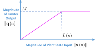
Figure 2: Energy limiter at the sensor.

The design of the limiter’s dynamic range $L\left(n\right)$ is very critical to the system performance. It’s clear that, due to the nonlinearity of the energy limiter, the magnitude information of $\mathbf{x}\left(n\right)$ will be partially lost when the limiter saturates, i.e., $\left\|\mathbf{x}\left(n\right)\right\|>L\left(n\right)$, which will greatly deteriorate the state estimation quality at the remote controller. We shall address how to design the limiter dynamic range $L\left(n\right)$ in Section III.

The sensor then transmits the magnitude-limited plant state $\mathbf{q}\left(n\right)$ to the remote controller over a wireless MIMO fading channel, and based on the limiter structure in (4), we have $\mathbf{q}^{T}\left(n\right)\mathbf{q}\left(n\right)\leq M^{2}$. Therefore, we restrict the energy availability constraint in (3) as follows:

$$M^{2}\mathrm{Tr}\left(\mathbf{F}^{H}(n)\mathbf{F}(n)\right)\tau\leq E(n).$$ (5)

III Dynamic MIMO Precoding via Lyapunov Optimization

In this section, we shall address the design of the energy limiter, and formulate the dynamic MIMO precoding problem to stabilize the unstable MIMO dynamic plant using Lyapunov optimization. We first have the following definition on the stability of the dynamic MIMO plant [15]:

Definition 1

(Stability of Dynamic MIMO Plant) The dynamic MIMO plant is stable if $\underset{N\rightarrow\infty}{\mathrm{limsup}}\frac{1}{N}\sum_{n=1}^{N}\mathbb{E}\left[\left\|\mathbf{x}\left(n\right)\right\|^{2}\right]<\infty,$ where the expectation is taken with respect to the randomness of the plant noise, the channel noise, the MIMO channel state, and the energy state.

III-A Virtual State Estimation Covariance Process

The nonlinear structure of the limiter introduces the nonlinear state estimation, and thus the evolution of the plant state estimation mean square error (MSE) is very difficult to be characterized explicitly. To get around this, we first establish a tight analytical bound on the state estimation MSE. Let $\hat{\mathbf{x}}\left(n\right)$ be the minimum mean square error (MMSE) MIMO plant state estimate at the controller. We have the following lemma, which gives an upper bound of the MSE of the plant state estimation $\mathbb{E}\left[\left\|\mathbf{x}\left(n\right)-\hat{\mathbf{x}}\left(n\right)\right\|^{2}\right]$

Lemma 1

(State Estimation MSE Bound of the Stochastic Dynamic MIMO Plant) For any control law $\mathbf{u}\left(n\right)$, the plant state estimation MSE $\mathbb{E}\left[\left\|\mathbf{x}\left(n\right)-\hat{\mathbf{x}}\left(n\right)\right\|^{2}\right]$ is bounded by a virtual state estimation MSE process according to:

$$\mathbb{E}\left[\left\|\mathbf{x}\left(n\right)-\hat{\mathbf{x}}\left(n\right)\right\|^{2}\right] \leq\mathbb{E}\left[\mathrm{Tr}\left(\boldsymbol{\Sigma}\left(n\right)\right)\right],$$ (6)

where $\boldsymbol{\Sigma}\left(n\right)$ is a virtual state estimation covariance process with the following dynamics:

$$\boldsymbol{\Sigma}\left(n+1\right)=\mathbf{A}\big{(}\boldsymbol{\Sigma}\left(n\right)-\gamma\left(n\right)\boldsymbol{\Sigma}\left(n\right)\big{(}\mathbf{\mathbf{\mathbf{\tilde{F}}}}^{a}\left(n\right)\big{)}^{H}\Big{(}\mathbf{\mathbf{\mathbf{\tilde{F}}}}^{a}\left(n\right)\boldsymbol{\Sigma}\left(n\right)$$

$$\hskip 28.45274pt\ \ \ \ \ \cdot\big{(}\mathbf{\mathbf{\mathbf{\tilde{F}}}}^{a}\left(n\right)\big{)}^{H}+\mathbf{I}\Big{)}^{-1}\mathbf{\mathbf{\mathbf{\tilde{F}}}}^{a}\left(n\right)\boldsymbol{\Sigma}\left(n\right)\big{)}\mathbf{A}^{T}+\mathbf{W},$$ (7)

with initial value $\boldsymbol{\Sigma}\left(0\right)=\mathbf{0}$, where $\gamma\left(n\right)=\mathbf{1}\left\{\left\|\mathbf{x}\left(n\right)\right\|\leq L\left(n\right)\right\}$, ${\normalcolor{\normalcolor\mathbf{\tilde{F}}(n)=\mathbf{H}(n)\mathbf{F}(n)g(n})}$, and $\mathbf{\mathbf{\mathbf{\tilde{F}}}}^{a}\left(n\right)=\begin{bmatrix}\mathbf{\mathbf{\tilde{F}}}\left(n\right)\\ \mathbf{\mathbf{\tilde{F}}}^{\dagger}\left(n\right)\end{bmatrix}$ is an augmented $2N_{c}\times K$ matrix.

Proof:

Please see Appendix -A. ∎

The upper bound of the MMSE in (6) can be achieved by using a low complexity state estimation $\widetilde{\hat{\mathbf{x}}}\left(n\right)=\mathbf{A}\widetilde{\hat{\mathbf{x}}}\left(n-1\right)+\gamma\left(n-1\right)\mathbf{A}\mathbf{K}\left(n-1\right)(\mathbf{y}^{a}\left(n-1\right)-\mathbf{\mathbf{\mathbf{\tilde{F}}}}^{a}\left(n-1\right)\widetilde{\hat{\mathbf{x}}}\left(n-1\right)),$ where $\mathbf{K}\left(n\right)=\boldsymbol{\Sigma}\left(n\right)(\mathbf{\mathbf{\mathbf{\tilde{F}}}}^{a}\left(n\right))^{H}(\mathbf{\mathbf{\mathbf{\tilde{F}}}}^{a}\left(n\right)\boldsymbol{\Sigma}\left(n\right)\big{(}\mathbf{\mathbf{\mathbf{\tilde{F}}}}^{a}\left(n\right)\big{)}^{H}+\mathbf{I})^{-1}$ and $\mathbf{y}^{a}\left(n\right)=\begin{bmatrix}\mathbf{\mathbf{y}}\left(n\right)\\ \mathbf{\mathbf{y}}^{\dagger}\left(n\right)\end{bmatrix}$.

We consider a control law of the form $\mathbf{u}(n)=-\boldsymbol{\Psi}\mathbf{A}\widetilde{\hat{\mathbf{x}}}\left(n\right)$ for the dynamic MIMO plant, where the feedback gain $\boldsymbol{\Psi}\mathbf{A}$ is chosen such that $\mathbf{A}-\mathbf{B}\boldsymbol{\Psi}\mathbf{A}$ is a Hurwitz matrix. Note that the certainty equivalent controller is given by $\mathbf{u}(n)=-\boldsymbol{\Xi}\widetilde{\hat{\mathbf{x}}}\left(n\right)$, where the feedback gain matrix is $\mathbf{\Xi}=\left(\mathbf{B}^{T}\mathbf{Z}\mathbf{B}+\mathbf{R}\right)^{-1}\mathbf{B}^{T}\mathbf{Z}$, $\mathbf{Z}$ satisfies the following discrete time algebraic Ricatti equation $\mathbf{Z}=\mathbf{A}^{T}\mathbf{Z}\mathbf{A}-\mathbf{A}^{T}\mathbf{Z}\mathbf{B}\left(\mathbf{B}^{T}\mathbf{Z}\mathbf{B}+\mathbf{R}\right)^{-1}\mathbf{B}^{T}\mathbf{Z}\mathbf{A}+\mathbf{P}$, and $\mathbf{P}\in\mathbb{S}_{+}^{K}$ and $\mathbf{R}\in\mathbb{S}_{+}^{D}$ are the weighting matrices for the plant state deviation cost and plant control cost of the LQG control associated with the certainty equivalent controller [17, 18]. Hence, one possible way to design such $\boldsymbol{\Psi}$ is let $\boldsymbol{\Psi}=-\left(\mathbf{B}^{T}\mathbf{Z}\mathbf{B}+\mathbf{R}\right)^{-1}\mathbf{B}^{T}\mathbf{Z}$. From Lemma 1, if we can achieve stability in the virtual state estimation error covariance process, i.e., $\underset{N\rightarrow\infty}{\mathrm{limsup}}\sum_{n=1}^{N}{\color[rgb]{0,0,1}\frac{{\normalcolor 1}}{{\normalcolor N}}}\mathbb{E}\left[\mathrm{Tr}\left(\boldsymbol{\Sigma}\left(n\right)\right)\right]<\infty$, then the actual plant state estimation MSE ($\mathbb{E}\left[\left\|\mathbf{x}\left(n\right)-\hat{\mathbf{x}}\left(n\right)\right\|^{2}\right]$) will also be bounded, which in turn leads to the bounded state process as in Definition 1. This is formally stated in the following Lemma.

Lemma 2

(Connection between Stability of $\boldsymbol{\Sigma}\left(n\right)$ and Stability of $\mathbf{x}\left(n\right)$) Under the control law $\mathbf{u}(n)=-\boldsymbol{\Psi}\mathbf{A}\widetilde{\hat{\mathbf{x}}}\left(n\right)$, if $\underset{N\rightarrow\infty}{\mathrm{limsup}}\frac{1}{N}\sum_{n=1}^{N}\mathbb{E}\left[\mathrm{Tr}\left(\boldsymbol{\Sigma}\left(n\right)\right)\right]<\infty$, then $\underset{N\rightarrow\infty}{\mathrm{limsup}}\frac{1}{N}\sum_{n=1}^{N}\mathbb{E}\left[\left\|\mathbf{x}\left(n\right)\right\|^{2}\right]<\infty.$

Proof:

Please see Appendix -B. ∎

Note that the evolution of the virtual state estimation MSE process $\boldsymbol{\Sigma}\left(n\right)$ depends on the dynamic MIMO precoder $\mathbf{F}\left(n\right)$ according to (7). As a result, we will focus on the design of dynamic MIMO precoding $\mathbf{F}\left(n\right)$ in the MIMO NCS to achieve stability of $\boldsymbol{\Sigma}\left(n\right)$.

III-B $\varepsilon$-Saturation Energy Limiter Design

The magnitude information of the plant state is partially lost when the limiter saturates. In conventional literature, bounded noise support is assumed, and hence saturation can be avoided with proper dynamic range design. In this work, we considered unbounded noise support, and hence saturation cannot be completely eliminated. Instead, we need to adapt the dynamic range $L\left(n\right)$ of the limiter to maintain a small probability of saturation $\varepsilon$. We have the following lemma on the design of the dynamic range of the limiter.

Lemma 3

($\varepsilon$-Saturation Limiter Dynamic Range Adaptation) Suppose the dynamic range $L\left(n\right)$ of the limiter evolves according to the following:

$$L\left(n\right)= \frac{1}{\sqrt{\varepsilon}}\left(1+\left\|\mathbf{A}-\mathbf{B}\boldsymbol{\Psi}\mathbf{A}\right\|\Theta\right)$$

$$\cdot\left(\left\|\mathbf{B}\boldsymbol{\Psi}\mathbf{A}\right\|\sqrt{\mathrm{Tr}\left(\boldsymbol{\Sigma}\left(n\right)\right)-\mathrm{Tr}\left(\mathbf{W}\right)}+\sqrt{\mathrm{Tr}\left(\mathbf{W}\right)}\right),$$ (8)

where

$$\Theta =\frac{1}{\mu_{min}\left(\mathbf{T}\right)}\bigg{(}\left\|\left(\mathbf{A}-\mathbf{B}\boldsymbol{\Psi}\mathbf{A}\right)^{T}\mathbf{Q}\right\|$$

$$+\left(\left\|\left(\mathbf{A}-\mathbf{B}\boldsymbol{\Psi}\mathbf{A}\right)^{T}\mathbf{Q}\right\|^{2}+\mu_{min}\left(\mathbf{T}\right)\left\|\mathbf{Q}\right\|\right)^{\nicefrac{{1}}{{2}}}\bigg{)}$$ (9)

is a constant ($\mathbf{Q}$ and $\mathbf{T}$ are any positive definite symmetric matrices such that $\left(\mathbf{A}-\mathbf{B}\boldsymbol{\Psi}\mathbf{A}\right)^{T}\mathbf{Q}\left(\mathbf{A}-\mathbf{B}\boldsymbol{\Psi}\mathbf{A}\right)-\mathbf{Q}=-\mathbf{T}$). Then

$$\mathrm{Pr}\left(\left\|\mathbf{x}\left(n\right)\right\|>L\left(n\right)\right) \leq\varepsilon$$ (10)

holds for any time slot $n$.

Proof:

Please see Appendix -C. ∎

Remark 1

(Computation of $L\left(n\right)$ at the Sensor) Since the input state process $\mathbf{x}\left(n\right)$ is a non-stationary random process, in order to maintain a small saturation probability $\varepsilon$, the dynamic range $L\left(n\right)$ of the limiter needs to be adaptive as in (8) to keep track of the instantaneous covariance of the input state process $\mathbf{x}\left(n\right)$. Note that the limiter’s dynamic range $L\left(n\right)$ is a function of the virtual state estimation covariance $\boldsymbol{\Sigma}\left(n\right)$. The sensor can obtain $\boldsymbol{\Sigma}\left(n\right)$ via the dynamics (7) based on the local information only without explicit signaling feedback, and hence it is implementation friendly. Due to the local availability of $\boldsymbol{\Sigma}\left(n\right)$ and $L\left(n\right)$ at the sensor, the MIMO precoding solution in Theorem 1 can be implemented at the sensor in a decentralized way.

III-C Dynamic MIMO Linear Precoding via Lyapunov Optimization

We focus on deriving a dynamic MIMO precoding policy to achieve stability of the virtual covariance process $\boldsymbol{\Sigma}\left(n\right)$ using Lyapunov techniques [19, 20]. Intuitively, a negative term in the Lyapunov drift is a stabilizing force that pulls the system state back to the equilibrium point. As a result, we shall design the dynamic MIMO precoder to maximize the negative Lyapunov drift to achieve stability under the renewable energy resource constraints.

We define a Lyapunov function as follows [20]:

$$V\left(n\right)=\frac{1}{2}\mathrm{Tr}\left(\boldsymbol{\Sigma}\left(n\right)\right)+\frac{1}{2}\left(E\left(n\right)-\theta\right)^{2}.$$ (11)

The associated Lyapunov drift is given by

$$\Lambda\left(\boldsymbol{\Sigma}\left(n\right)\right)$$

$$=\mathbb{E}\left\{\left.V\left(n+1\right)-V\left(n\right)\right|\boldsymbol{\Sigma}\left(n\right)\right\},$$ (12)

where the expectation $\mathbb{E}$ is w.r.t. the randomness of the channel state and the energy state under a given MIMO precoding rule $\mathbf{F}(n)$. We have the following lemma on the Lyapunov drift.

Lemma 4

(Lyapunov Drift) Given a MIMO precoding rule $\mathbf{F}(n)$, the Lyapunov drift can be upper bounded as follows:

$$\Lambda\left(\boldsymbol{\Sigma}\left(n\right)\right)\leq\frac{1}{2}\mathrm{Tr}(\mathbf{W})+\mathbb{E}\left[\left(\alpha\left(n\right)+\theta\right)^{2}\right]$$

$$+\mathbb{E}\bigg{\{}\underbrace{\frac{1}{2}\left\|\mathbf{A}\mathbf{A}^{T}\right\|\bigg{[}\varepsilon\mathrm{Tr}\left(\boldsymbol{\Sigma}\left(n\right)\right)}_{"bad"\ term\ causing\ instability}+$$

$$\underbrace{\mathrm{Tr}\left(2\frac{M^{2}}{L^{2}(n)}\mathrm{Re}\left\{\mathbf{F}^{H}\left(n\right)\mathbf{H}^{H}(n)\mathbf{H}(n)\mathbf{F}\left(n\right)\right\}+\boldsymbol{\Sigma}\left(n\right)^{-1}\right)^{-1}}_{"bad"\ term\ causing\ instability}\bigg{]}$$

$$+\underbrace{M^{2}\mathrm{Tr}\left(\mathbf{F}^{H}(n)\mathbf{F}(n)\right)\tau\left(\theta-E\left(n\right)\right)}_{"bad"\ term\ causing\ instability}$$

$$-\underbrace{\frac{1}{2}\mathrm{Tr}\left(\boldsymbol{\Sigma}\left(n\right)\right)}_{\underset{(stabilizing\ force)}{"good"\ term}}\bigg{\}}\bigg{|}\boldsymbol{\Sigma}\left(n\right)\bigg{\}}.$$ (13)

Proof:

Please see Appendix -D. ∎

The first expectation on the R.H.S of (13) is taken w.r.t. the randomness of energy arrival, the second expectation on the R.H.S of (13) is taken w.r.t. the randomness of both the channel state and the energy state under given $\boldsymbol{\Sigma}\left(n\right)$ and MIMO precoding rule $\mathbf{F}(n)$. Note that the negative Lyapunov drift plays a central role when applying the Lyapunov drift theory to analyze the stability of dynamic systems. Intuitively, the negative Lyapunov drift is a stabilizing force that pulls the system state back to the equilibrium point. The drift term in equation (13) that contributes to positive Lyapunov drift is bracketed as a “bad” term for stabilization of $\boldsymbol{\Sigma}\left(n\right)$, because positive Lyapunov drift leads to instability of $\boldsymbol{\Sigma}\left(n\right)$. On the contrary, the drift term that contributes to negative Lyapunov drift is bracketed as a “good” term for stabilization of $\boldsymbol{\Sigma}\left(n\right)$, because negative Lyapunov drift is the stabilizing force for the stability of $\boldsymbol{\Sigma}\left(n\right)$. Hence, we focus on deriving a dynamic MIMO precoder to minimize the drift (13). This is equivalent to considering the following optimization problem:

Problem 1

(MIMO Precoding via Lyapunov Optimization) For given realizations $E(n)=E$, $\boldsymbol{\Sigma}\left(n\right)=\boldsymbol{\Sigma}$, and $\mathbf{H}(n)=\mathbf{H}$, the MIMO precoding $\mathbf{F}\left(n\right)$ is given by the solution of the following problem:

$$\underset{\mathrm{\mathbf{F}}\left(n\right)}{\mathrm{min}}\ \ M^{2}\mathrm{Tr}\left(\mathbf{F}^{H}(n)\mathbf{F}(n)\right)\tau\left(\theta-E\right)$$

$$+\frac{\left\|\mathbf{A}\mathbf{A}^{T}\right\|}{2}\mathrm{Tr}\left(2\frac{M^{2}}{L^{2}(\boldsymbol{\Sigma})}\mathrm{Re}\left\{\mathbf{F}^{H}(n)\mathbf{H}^{H}\mathbf{H}\mathbf{F}(n)\right\}+\boldsymbol{\Sigma}^{-1}\right)^{-1}$$

$$s.t.\ \ M^{2}\mathrm{Tr}\left(\mathbf{F}^{H}(n)\mathbf{F}(n)\right)\tau\leq E,$$

where $L(\boldsymbol{\Sigma})$ is given in (8).

Challenge 2: Closed-form Dynamic MIMO Precoder Design.

While Problem 1 is equivalent to a convex problem, it is still very challenging to obtain closed-form solution. This is due to the tight coupling in the objective function (involving a mixture of real, trace and inverse).

IV Event-Driven Energy Harvesting and MIMO Precoding Solution

In this section, we shall give the MIMO precoding solution to Problem 1 and discuss its structural properties.

IV-A Drift Minimizing MIMO Precoder

The underlying structure of the objective function of Problem 1 provides some key insights into the MIMO precoding solution structure. Specifically, if $\mathrm{Re}\left\{\mathbf{F}^{H}(n)\mathbf{H}^{H}\mathbf{H}\mathbf{F}(n)\right\}$, $\boldsymbol{\Sigma}^{-1}$ and $\mathbf{F}^{H}(n)\mathbf{F}(n)$ can be simultaneously diagnalized, then the objective function is substantially simplified because the matrix operations will only involve diagonal matrices. This may be feasible if $\mathbf{F}(n)$ can be expressed as a product of three matrices, where the leftmost matrix is the Hermitian of the right singular matrix of $\mathbf{H}$ and the rightmost matrix is the Hermitian of the left right singular matrix of $\boldsymbol{\Sigma}$. Inspired by this observation, let the singular value decomposition of the matrix of $\mathbf{H}$ be $\mathbf{H}=\mathbf{V}\boldsymbol{\Pi}\mathbf{U}^{H}$, where ${\normalcolor\mathbf{V}\in\mathbb{C}^{N_{c}\times N_{c}}}$ and $\mathbf{U}\in\mathbb{C}^{N_{s}\times N_{s}}$ are unitary matrices, and $\boldsymbol{\Pi}$ is a rectangular diagonal matrix with diagonal elements in a descending order. Denote $\boldsymbol{\Pi}_{K}$ as the leading principal minor of order $K$ of $\boldsymbol{\Pi}$. Let the eigenvalue decomposition of $\boldsymbol{\Sigma}^{-1}$ be $\boldsymbol{\Sigma}=\mathbf{S}\boldsymbol{\Lambda}\mathbf{S}^{T}$, where $\mathbf{S}\in\mathbb{C}^{K\times K}$ is an orthogonal matrix, and $\boldsymbol{\Lambda}\in\mathbb{\mathbb{R}}^{K\times K}$ is diagonal with diagonal elements in a descending order. Then the drift-minimizing solution of Problem 1 is given as follows.

Theorem 1

(Drift-Minimizing Solution) The drift-minimizing MIMO precoding is as follows:

• Dormant Mode: If $\theta\mathbf{I}-\big{(}\frac{\left\|\mathbf{A}\mathbf{A}^{T}\right\|\boldsymbol{\Lambda}^{2}\boldsymbol{\Pi}_{K}^{2}}{\tau L^{2}(\boldsymbol{\Sigma})}+E\mathbf{I}\big{)}$ is positive definite, then $\mathbf{F}^{\ast}\left(n\right)=\mathbf{0}.$

• Active Mode: If $\theta\mathbf{I}-\big{(}\frac{\left\|\mathbf{A}\mathbf{A}^{T}\right\|\boldsymbol{\Lambda}^{2}\boldsymbol{\Pi}_{K}^{2}}{\tau L^{2}(\boldsymbol{\Sigma})}+E\mathbf{I}\big{)}$ is not positive definite, then

  $$\mathbf{F}^{\ast}\left(n\right)=\frac{L(\boldsymbol{\Sigma})}{M}\mathbf{U}$$

  $$\cdot\bigg{[}\begin{array}[]{c}\boldsymbol{\Pi}_{K}^{-1}\Big{(}\frac{1}{2}\Big{[}\frac{\boldsymbol{\Pi}_{K}}{L\left(\boldsymbol{\Sigma}\right)}\sqrt{\frac{\left\|\mathbf{A}\mathbf{A}^{T}\right\|}{\left(\left[\theta-E\right]^{+}+\beta\right)\tau}}-\boldsymbol{\Lambda}^{-1}\Big{]}^{+}\Big{)}^{\nicefrac{{1}}{{2}}}\mathbf{S}^{T}\\ \mathbf{0}\end{array}\bigg{]},$$

  where $\beta$ is given by (14).

  $$\beta=\begin{cases}chosen\ such\ that\ &if\ \mathrm{Tr}\Big{(}\frac{1}{2}\boldsymbol{\Pi}_{K}^{-2}\Big{[}\frac{\boldsymbol{\Pi}_{K}}{L\left(\boldsymbol{\Sigma}\right)}\sqrt{\frac{\left\|\mathbf{A}\mathbf{A}^{T}\right\|}{\left(\theta-E\right)\tau}}-\boldsymbol{\Lambda}^{-1}\Big{]}^{+}\Big{)}\geq\frac{E}{\tau L^{2}(\boldsymbol{\Sigma})};\\ M^{2}\mathrm{Tr}\left({\color[rgb]{0,0,1}{\normalcolor\left(\mathbf{F}^{\ast}(n)\right)^{H}\mathbf{F}^{\ast}(n)}}\right)\tau=E,\\ \\ 0,&otherwise.\end{cases}$$ (14)

  
  

Proof:

Please see Appendix D. ∎

Remark 2

(Interpretation on the Structure of the Drift-minimizing MIMO Precoding Solution)

Event-driven Structure: The MIMO precoding solution in Theorem 1 also has an event-driven structure, in the sense that the sensor either transmits or shuts down aperiodically depending only on whether the dynamic threshold $\theta\mathbf{I}-\big{(}\frac{\left\|\mathbf{A}\mathbf{A}^{T}\right\|\boldsymbol{\Lambda}^{2}\boldsymbol{\Pi}_{K}^{2}}{\tau L^{2}(\boldsymbol{\Sigma})}+E\mathbf{I}\big{)}$ is positive definite or not.

• Large $\|\boldsymbol{\Pi}_{K}\|$ (good channel condition) or large $E$ (sufficient energy in the storage) leads to active mode of the sensor, which means it is better that the sensor be active when there are good transmission opportunities.

• Large MIMO plant state estimation error implies large $\|\boldsymbol{\Sigma}\|$, as shown in Lemma 1, which also leads to the active mode of the sensor. This is because a large MIMO plant state estimation error means high transmission urgency and hence it is better that the sensor be active.

Figure 3 illustrates a sample path of the state estimation error and transition between the active and dormant modes. It can be observed that the state estimation error ${\normalcolor\left\|\mathbf{x}\left(n\right)-\hat{\mathbf{x}}\left(n\right)\right\|^{2}}$ increases during the dormant modes and is reset to a low value during the active modes. As such, the MIMO precoding solution has an event-driven structure with aperiodic reset of state estimation error.

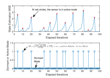
Figure 3: Sample path of state estimation error and transitions between active and dormant modes. The system parameters are configured as follows:$\mathbf{A}=\left(\begin{array}[]{cc}1.3&0.1\\ -0.2&1.2\end{array}\right)$, $\mathbf{\mathbf{B}}=\mathrm{diag(1,1)}$, $\mathbf{\mathbf{W}}=\mathrm{diag(1,2)}$, $\mathbf{\mathbf{Q}}=\mathrm{diag(1,1)}$, $\mathbf{\mathbf{\Psi}}=\mathrm{diag(0.25,0.25)}$, $\varepsilon=0.01$, $M=1$, $N_{s}=3$, $N_{c}=2$, $\tau=0.01$, $\mathbb{E}\left[\alpha\right]=5$ and $\theta=30.$

Note that the virtual state estimation covariance $\boldsymbol{\Sigma}$ can be decomposed as $\boldsymbol{\Sigma}=\mathbf{S}\boldsymbol{\Lambda}\mathbf{S}^{H}$ with $\mathbf{S}$ and $\boldsymbol{\Lambda}$ being unitary and diagonal, respectively. Hence, each diagonal element of $\boldsymbol{\Lambda}$ corresponds to a subsystem with $\boldsymbol{\Lambda}_{ii}$ as the state estimation error of the $i$-th subsystem.

Dynamic Spatial Channel Activation Structure: The MIMO precoding solution $\mathbf{F}^{\ast}\left(n\right)$ dynamically activates the spatial channels. Specifically, whether the $i$-th spatial channel (the spatial channel corresponds to the $i$-th subsystem) is activated or not depends only on whether the dynamic threshold $\frac{\left\|\mathbf{A}\mathbf{A}^{T}\right\|\left(\boldsymbol{\Lambda}\boldsymbol{\Pi}_{K}\right)_{ii}^{2}}{\tau L^{2}(\boldsymbol{\Sigma})}-\left[\theta-E\right]^{+}-\beta$ is positive or not.

Eigenvalue Water-filling Structure: The MIMO precoding solution $\mathbf{F}^{\ast}\left(n\right)$ also has an eigenvalue water-filling structure. Specifically, for the $i$-th subsystem, $\frac{\left(\boldsymbol{\Pi}_{K}\right)_{ii}}{L\left(\boldsymbol{\Sigma}\right)}\sqrt{\frac{\left\|\mathbf{A}\mathbf{A}^{T}\right\|}{\left(\left[\theta-E\right]^{+}+\beta\right)\tau}}$ is the dynamic water level which adapts to the virtual state estimation covariance $\boldsymbol{\Sigma}$, energy storage $E$, and the $i$-th spatial channel $\left(\boldsymbol{\Pi}_{K}\right)_{ii}$, and $\left(\boldsymbol{\Lambda}\right)_{ii}^{-1}$ is the dynamic seabed level. Large energy storage (i.e., large $E$) or better channel condition of the $i$-th spatial channel (i.e., large $\left(\boldsymbol{\Pi}_{K}\right)_{ii}$) will lead to a high water level which will allow the sensor to allocate more transmission energy for the $i$-th subsystem. High transmission urgency (i.e., large $\left(\boldsymbol{\Lambda}\right)_{ii}$) will lead to a low seabed level, which induces more energy to be allocated to the subsystem.

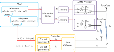
(a) System model of the noisy decoupled plant system.

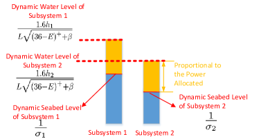
(b) Eigenvalue water-filling structure.

Figure 4: Illustrations of the system model and the eigenvalue water-filling structure of the drift-minimizing MIMO precoding solution in Example 1.

Remark 3

(Comparison with Traditional MIMO Precoding Solutions)

The traditional waterfilling MIMO precoding solution [21] that maximizing the physical layer capacity has the form $\mathbf{F}\left(n\right)=\mathbf{U}\mathbf{\Upsilon}$, where $\left(\mathbf{\Upsilon}\right)_{ii}=\left[\gamma-\frac{1}{\left(\boldsymbol{\Pi}_{K}\right)_{ii}}\right]^{+}$ for all $i=1,\ldots,K$, the water level $\gamma$ is chosen such that $\sum_{i=i}^{K}\left(\mathbf{\Upsilon}\right)_{ii}=\frac{E\left(n\right)}{M^{2}\tau}$, and the other elements of $\mathbf{\Upsilon}$ are zero. The traditional waterfilling solution is only adapted to the channel state. The waterfilling solution under energy harvesting constraints in [22] maximizes the physical layer capacity subject to the energy causality constraints, and the solution has the form $\mathbf{F}\left(n\right)=\mathbf{U}\mathbf{\Upsilon}$, where $\left(\mathbf{\Upsilon}\right)_{ii}=\left[\frac{1}{\sum_{j=i}^{K+1}\lambda_{j}-\sum_{j=i}^{K}\mu_{j}}-\frac{1}{\left(\boldsymbol{\Pi}_{K}\right)_{ii}}\right]^{+}$ for all $i=1,\ldots,K$, $\lambda_{j}$ are the Lagrange multiplier that enforce energy causality and $\mu_{j}$ are the Lagrange multipliers that enforce no-energy overflow conditions. Similarly, the waterfilling solution under energy harvesting constraints also only adapts to the energy state and channel state. In contrast, the proposed MIMO precoding solution is truly dynamic and adaptive to the MIMO channel state, sensor energy state and plant state transmission urgency. It is noticed that the traditional waterfilling solution and the waterfilling solution with energy harvesting constraints both fail to exploit plant state transmission urgency and therefore, they have inferior performance as shown in Section VI.

IV-B Application Example

We consider the following simple toy example to illustrate the structural properties of the MIMO precoding solution.

Example 1

(Noisy Decoupled Plant System) We consider an aggregation of two decoupled SISO plant subsystems as illustrated in Figure 4. The dynamics of the two subsystems are given by:

$$x_{1}\left(n+1\right)=1.6x_{1}\left(n\right)+u_{1}\left(n\right)+w_{1}\left(n\right)\ \ \ (Subsystem\ 1)$$

$$x_{2}\left(n+1\right)=1.1x_{2}\left(n\right)+u_{2}\left(n\right)+w_{2}\left(n\right)\ \ \ (Subsystem\ 2),$$

where $w_{1}\left(n\right)$ and $w_{2}\left(n\right)$ are independent Gaussian random noise with zero mean and covariance 1. Let the control rule be $u_{1}\left(n\right)=-0.8\hat{x}_{1}\left(n\right)$ and $u_{2}\left(n\right)=-0.55\hat{x}_{2}\left(n\right)$. Let $\theta=36$, $\tau=1$ and the parameters of the $\varepsilon$-saturation limiter be $\varepsilon=0.1$, $M=1$ and $\mathbf{\mathbf{Q}}=\mathbf{I}$. The energy-harvesting sensor observes the limiter output $\mathbf{q}\left(n\right)=\left(q_{1}\left(n\right),q_{2}\left(n\right)\right)$, applies a precoder $\mathbf{F}=\left[\begin{array}[]{cc}f_{11}&f_{12}\\ f_{21}&f_{22}\end{array}\right]$ and sends the magnitude-limited plant state to the controllers via a decoupled parallel channel $\mathbf{H}=\left(\begin{array}[]{cc}h_{1}&0\\ 0&h_{2}\end{array}\right)$. This corresponds to a special case of the NCS system with $K=2$, $N_{s}=2$, $N_{c}=2$, $\mathbf{A}=\left(\begin{array}[]{cc}1.6&0\\ 0&1.1\end{array}\right)$, $\mathbf{B}=\mathbf{\mathbf{W}}=\mathbf{I}$, and $\boldsymbol{\Psi}=\frac{1}{2}\mathbf{I}$.

According to Theorem 1, the MIMO precoding solution for Example 1 is given by:

$$\mathbf{F}^{\ast}\left(n\right)= \frac{L}{\sqrt{2}}\mathrm{diag}\bigg{\{}\frac{1}{\left|h_{1}\right|}\sqrt{\left[\frac{1.6\left|h_{1}\right|}{L\sqrt{\left(36-E\right)^{+}+\beta}}-\frac{1}{\sigma_{1}}\right]^{+}}$$

$$,\frac{1}{\left|h_{2}\right|}\sqrt{\left[\frac{1.6\left|h_{2}\right|}{L\sqrt{\left(36-E\right)^{+}+\beta}}-\frac{1}{\sigma_{2}}\right]^{+}}\bigg{\}},$$

where $\boldsymbol{\Sigma}_{n}=\left[\begin{array}[]{cc}\sigma_{1}&0\\ 0&\sigma_{2}\end{array}\right]$ is the virtual state estimation covariance matrix, $L=22.36+7.91\sqrt{\sigma_{1}+\sigma_{2}-2}$, and $\beta=0$ if $\left\|\mathbf{F}^{\ast}\left(n\right)\right\|_{F}^{2}<E$, else $\beta$ is chosen such that $\left\|\mathbf{F}^{\ast}\left(n\right)\right\|_{F}^{2}=E$.

• When the Sensor has to be Active? Based on the event-driven structure in Remark 3, the sensor will be activated if either $36-E-\frac{2.56h_{1}^{2}\sigma_{1}^{2}}{\left(22.36+7.91\sqrt{\sigma_{1}+\sigma_{2}-2}\right)^{2}}$ or $36-E-\frac{2.56h_{2}^{2}\sigma_{2}^{2}}{\left(22.36+7.91\sqrt{\sigma_{1}+\sigma_{2}-2}\right)^{2}}$ is negative. Therefore, better channel condition (large $h_{1}$ or $h_{2}$), large energy storage $E$ or increased transmission urgency (large $\sigma_{1}$ or $\sigma_{2}$) will lead to the active mode of the sensor.

• Which Spatial Channel to Turn On? Suppose $h_{1}=4$ and $\sigma_{1}$ = 70, Figure 5 illustrates the number of spatial channels activated at different regions of the state space $\left(h_{2},\sigma_{2}\right)$ for different $E$. It can be observed that the region where both spatial channels are turned on enlarges as the available energy $E$ increases. This is reasonable because large $E$ means a good transmission opportunity which allows more spatial channels to be activated.

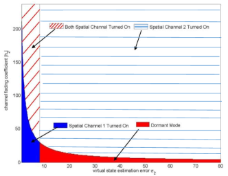
(a) Decision Region of Spatial Channel Activation w.r.t. $h_{2}$ and $\sigma_{2}$ with $h_{1}=4$, $\sigma_{1}=70$ and $E=12$.

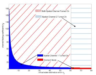
(b) Decision Region of Spatial Channel Activation w.r.t. $h_{2}$ and $\sigma_{2}$ with $h_{1}=4$, $\sigma_{1}=70$ and $E=20$.

Figure 5: Decision Region of Spatial Channel Activation w.r.t. $h_{2}$ and $\sigma_{2}$ for different $E$ with $h_{1}=4$ and $\sigma_{1}=70$.

V STABILITY ANALYSIS

In this section, we derive the sufficient condition for NCS stability under the drift-minimizing MIMO linear precoding solution in Theorem 1, and analyze the MIMO plant state estimation performance.

V-A Sufficient Condition for NCS Stability

Instability measures of the unstable dynamic plants provide key information directly related to stabilizability and performance limitations. One of the key measures that has been proposed in the literature for measuring the instability of the unstable dynamic plants is defined as the product of the modulus of the unstable eigenvalues of matrix $\mathbf{A}$ [23, 24], i.e.,

$$\mathcal{M}\left(\mathbf{A}\right)=\prod_{i=1}^{K}\mathrm{\mathrm{max\left(1,\left|\mu_{i}\left(\mathbf{A}\right)\right|\right)}}.$$ (15)

In this section, we shall establish a sufficient condition for NCS stability under the proposed MIMO precoding policy in terms of the instability measure $\mathcal{M}\left(\mathbf{A}\right)$, the energy arrival $\alpha\left(n\right)$ as well as the battery capacity $\theta$. The sufficient condition for NCS stability is summarized in Theorem 2.

Theorem 2

(Sufficient Condition for NCS Stability) If the following condition is satisfied:

$$\mathbb{E}\left[\frac{1}{\alpha}\right]+\frac{1}{\theta}<\underset{\xi}{\mathrm{max}}\frac{1-\left(\varepsilon+K\mathrm{Pr}\left(\tilde{\pi}<\xi\right)\right)\mathcal{M}\left(\mathbf{A}\mathbf{A}^{T}\right)}{\delta^{2}K\tau\mathbb{E}\left[\left.\tilde{\pi}^{-1}\right|\tilde{\pi}\geq\xi\right]\mathcal{M}\left(\mathbf{A}\right){\normalcolor\mathcal{M}\left(\mathbf{A}\mathbf{A}^{T}\right)}},$$ (16)

where $\tilde{\pi}=\frac{\pi}{\mathrm{Tr}\left(\boldsymbol{\Pi}_{K}^{-1}\right)}$ and $\pi$ is the unordered singular value of $\mathbf{H}$, $\delta=\sqrt{\frac{2}{\varepsilon}}\left(1+\left\|\mathbf{A}-\mathbf{B}\boldsymbol{\Psi}\mathbf{A}\right\|\Theta\right)\left\|\mathbf{B}\boldsymbol{\Psi}\right\|\left\|\mathbf{A}\right\|$ and $\Theta$ is a constant given in Lemma 3, then the dynamic MIMO plant is stable.

Proof:

Please see Appendix E. ∎

The sufficient condition in Theorem 2 delivers some key design insights into the dynamic MIMO plant system. Specifically, we have the following system design insights.

• Limiter Requirement: The $\varepsilon$-saturation limiter should be carefully designed such that the saturation probability $\varepsilon$ obeys $\varepsilon<\mathcal{M}\left(\mathbf{A}\mathbf{A}^{T}\right)^{-1}-K\mathrm{Pr}\left(\tilde{\pi}<\xi^{\ast}\right)$, where $\xi^{\ast}=\underset{\xi}{\mathrm{arg}\ \mathrm{max}}\ \frac{1-\left(\varepsilon+K\mathrm{Pr}\left(\tilde{\pi}<\xi\right)\right)\mathcal{M}\left(\mathbf{A}\mathbf{A}^{T}\right)}{\delta^{2}K\tau\mathbb{E}\left[\left.\tilde{\pi}^{-1}\right|\tilde{\pi}\geq\xi\right]\mathcal{M}\left(\mathbf{A}\right)\mathcal{M}\left(\mathbf{A}\mathbf{A}^{T}\right)}$. This means that if the MIMO plant is very unstable (i.e., large $\mathcal{M}\left(\mathbf{A}\right)$), the limiter should be designed with very small saturation probability to guarantee stability.

• Battery Capacity Requirement: The battery capacity $\theta$ should obey $\theta>\frac{\delta^{2}K\tau\mathbb{E}\left[\left.\tilde{\pi}^{-1}\right|\tilde{\pi}\geq\xi\right]\mathcal{M}\left(\mathbf{A}\right)\mathcal{M}\left(\mathbf{A}\mathbf{A}^{T}\right)}{1-\left(\varepsilon+K\mathrm{Pr}\left(\tilde{\pi}<\xi^{\ast}\right)\right)\mathcal{M}\left(\mathbf{A}\mathbf{A}^{T}\right)}$. This means the more unstable the MIMO plant is, the larger the capacity of the energy storage devices is required.

• Energy arrival requirement: The sufficient condition also implies that in order to achieve stability, there is a requirement on the minimum average energy arrival rate, i.e., $\mathbb{E}\left[\alpha\right]\geq\left(\mathbb{E}\left[\frac{1}{\alpha}\right]\right)^{-1}>\left(\frac{1-\left(\varepsilon+K\mathrm{Pr}\left(\tilde{\pi}<\xi\right)\right)\mathcal{M}\left(\mathbf{A}\mathbf{A}^{T}\right)}{\delta^{2}K\tau\mathbb{E}\left[\left.\tilde{\pi}^{-1}\right|\tilde{\pi}\geq\xi\right]\mathcal{M}\left(\mathbf{A}\right)\mathcal{M}\left(\mathbf{A}\mathbf{A}^{T}\right)}-\frac{1}{\theta}\right)^{-1}$, and larger average energy arrival rate (stronger energy harvesting capability) is required for the more unstable MIMO plant.

The sufficient condition (16) is not difficult to check because it is expressed in terms of key system parameters from individual components of the system. For example, In (16), $\delta$, $K$, $\mathcal{M}\left(\mathbf{A}\right)$ and $\mathcal{M}\left(\mathbf{A}\mathbf{A}^{T}\right)$ are the parameters from the MIMO dynamic plant. $\mathbb{E}\left[\frac{1}{\alpha}\right]$ is the statistical parameters for renewable energy source, which can be obtained from offline measurements. $\theta$ is the battery size of the sensor. $\varepsilon$ is the sensor limiter saturation probability. $\mathrm{Pr}\left(\tilde{\pi}<\xi\right)$ and $\mathbb{E}\left[\left.\tilde{\pi}^{-1}\right|\tilde{\pi}\geq\xi\right]$ are the statistical parameters for the MIMO fading channel, which again can be obtained from offline measurements.

Remark 4

In [25, 26], the authors show that to achieve stability there is a minimum data rate requirement in terms of the instability measure (15). In our scenario, if there is no sufficient energy storage, the sensor tends to be in sleep mode and there is no data transmission between the sensor and the controller. Hence, the available transmission energy at the sensor will affect the communication data rate. This intuitively indicates that to achieve stability there shall exist some requirement on the available transmission energy at the sensor. This effect is shown in the sufficient condition (16), where there is a requirement on the minimum average energy arrival rate in terms of instability measure (15).

V-B State Estimation MSE Performance

We are interested in analyzing the achievable state estimation MSE using the proposed MIMO linear precoding policy. This is summarized in the theorem below.

Theorem 3

(MSE of State Estimation Error) If the sufficient condition for NCS stability (16) is satisfied, then the MSE satisfies:

$$\underset{N\rightarrow\infty}{\mathrm{limsup}}\frac{1}{N}\sum_{n=0}^{N-1}\mathbb{E}\left[\left\|\mathbf{x}\left(n\right)-\hat{\mathbf{x}}\left(n\right)\right\|^{2}\right]$$

$$\leq\frac{1}{\eta}\bigg{(}1+K\tau\frac{\delta^{2}}{\left\|\mathbf{B}\boldsymbol{\Psi}\right\|^{2}}\mathbb{E}\left[\left.\tilde{\pi}^{-1}\right|\tilde{\pi}\geq\xi\right]\left(\mathbb{E}\left[\frac{1}{\alpha}\right]+\frac{1}{\theta}\right)$$

$$\cdot\mathcal{M}\left(\mathbf{A}\right)\mathcal{M}\left(\mathbf{A}\mathbf{A}^{T}\right)\bigg{)}\mathrm{Tr}\left(\mathbf{W}\right)+\frac{\theta^{2}}{\eta},$$ (17)

where

$$\eta=1-\varepsilon\mathcal{M}\left(\mathbf{A}\mathbf{A}^{T}\right)-K\mathrm{Pr}\left(\tilde{\pi}<\xi^{\ast}\right)\mathcal{M}\left(\mathbf{A}\mathbf{A}^{T}\right)$$

$$-\left(\mathbb{E}\left[\frac{1}{\alpha}\right]+\frac{1}{\theta}\right)KT\delta^{2}\tau\mathbb{E}\left[\left.\tilde{\pi}^{-1}\right|\tilde{\pi}\geq\xi^{\ast}\right]\mathcal{M}\left(\mathbf{A}\right)\mathcal{M}\left(\mathbf{A}\mathbf{A}^{T}\right).$$ (18)

Proof:

Please see Appendix G. ∎

The state estimation performance bound (17) reveals the fact that large average energy arrival rate (small $\mathbb{E}\left[\frac{1}{\alpha}\right]$) and good MIMO channel quality (small $\mathbb{E}\left[\left.\tilde{\pi}^{-1}\right|\tilde{\pi}\geq\xi^{\ast}\right]$ and $\mathrm{Pr}\left(\tilde{\pi}<\xi^{\ast}\right)$) will result in a better state estimation performance.

VI Numerical Results

In this section we compare the performance of the proposed MIMO linear precoding scheme with the following baselines via numerical simulations.

• Baseline 1 (MIMO Water-filling Precoding Maximizing Capacity) [27, 21]: The MIMO precoding action is given by $\mathbf{F}\left(n\right)=\mathbf{U}\mathbf{\Upsilon}$, where $\mathbf{\Upsilon}\in\mathbb{R}^{N_{t}\times K}$, $\left(\mathbf{\Upsilon}\right)_{ii}=\left[\gamma-\frac{1}{\left(\boldsymbol{\Pi}_{K}\right)_{ii}}\right]^{+}$ for all $i=1,\ldots,K$, the water level $\gamma$ is chosen such that $\sum_{i=i}^{K}\left(\mathbf{\Upsilon}\right)_{ii}=\frac{E\left(n\right)}{M^{2}\tau}$, and the other elements of $\mathbf{\Upsilon}$ are zero. This corresponds to the physical layer capacity maximizing solution.

• Baseline 2 (Periodic MIMO Water-filling Precoding): The sensor is periodically activated for transmission with a fixed period of $T$ . The sensor adopts the MIMO water-filling precoding in baseline 1 when it transmits.

• Baseline 3 (MIMO Water-filling Precoding Minimizing MSE) [5]: The MSE minimizing precoding solution is given by $\mathbf{F}\left(n\right)=\mathbf{U}\mathbf{\Upsilon}$, where $\left(\mathbf{\Upsilon}\right)_{ii}=\left[\frac{\gamma}{\sqrt{\left(\boldsymbol{\Pi}_{K}\right)_{ii}}}-\frac{1}{\left(\boldsymbol{\Pi}_{K}\right)_{ii}}\right]^{+}$ for all $i=1,\ldots,K$, and $\gamma$ is chosen such that $\sum_{i=i}^{K}\left(\mathbf{\Upsilon}\right)_{ii}=\frac{E\left(n\right)}{M^{2}\tau}$, and the other elements of $\mathbf{\Upsilon}$ are zero.

• Baseline 4 (MIMO Water-filling Precoding Maximizing Capacity with Constant Power Supply): The MIMO precoding is in the same form as Baseline 1 except that the MIMO precoding is supplied with constant power $\mathbb{E}\left[\alpha\right]$, i.e., $\sum_{i=i}^{K}\left(\mathbf{\Upsilon}\right)_{ii}=\frac{\mathbb{E}\left[\alpha\right]}{M^{2}\tau}$, where the constant $\mathbb{E}\left[\alpha\right]$ is the average energy arrival.

• Baseline 5 (MIMO Water-filling Precoding Minimizing MSE with Constant Power Supply): The MIMO precoding is in the same form as Baseline 3 except that the MIMO precoding is supplied with constant power $\mathbb{E}\left[\alpha\right]$, i.e., $\sum_{i=i}^{K}\left(\mathbf{\Upsilon}\right)_{ii}=\frac{\mathbb{E}\left[\alpha\right]}{M^{2}\tau}$, where the constant $\mathbb{E}\left[\alpha\right]$ is the average energy arrival.

We consider a MIMO with parameters: $\mathbf{A}=\left(\begin{array}[]{cc}1.3&0.1\\ -0.2&1.2\end{array}\right)$, $\mathbf{\mathbf{B}}=\mathrm{diag(1,1)}$, $\mathbf{\mathbf{W}}=\mathrm{diag(1,2)}$, $\mathbf{\mathbf{Q}}=\mathrm{diag(1,1)}$, $\mathbf{\mathbf{\Psi}}=\mathrm{diag(0.25,0.25)}$, $\varepsilon=0.05$, $M=1$, $N_{s}=3$, $N_{c}=2$, $T=3\tau$ and $\tau=0.01s$. The harvestable energy process $\alpha\left(n\right)$ is assumed to be Poisson distributed. The MIMO channel $\mathbf{H}\left(n\right)$ is a $2\times 3$ matrix with each element being i.i.d. complex Gaussian distributed with zero mean and unit variance. The MIMO plant dynamics $\mathbf{A}$ has unstable eigenvalues with instability measure $\mathcal{M}\left(\mathbf{A}\right)=1.58$. The simulation is Monte Carlo simulation and for a given pair of average energy arrival $\mathbb{E}\left[\alpha\right]$ and battery capacity $\theta$, we simulate 5000 sample paths of plant state evolution and estimation, and each sample path contains 300 time slots. The system parameter configurations, namely the harvestable energy process $\alpha\left(n\right)$, battery capacity $\theta$, MIMO channel $\mathbf{H}$, limiter saturation probability $\varepsilon$, and limiter parameter $\delta$ of Baseline 1-3 are the same as the proposed scheme, and the system parameter configurations satisfy the stability condition (16) in Theorem 2. The Baseline 1-3 and the proposed scheme also satisfy the peak power restriction and the energy harvesting constraints.

VI-A State Estimation MSE Versus Battery Capacity $\theta$

Figure 6 illustrates the normalized MSE of the state estimation error versus the sensor battery capacity $\theta$ under the average energy arrival $\mathbb{E}\left[\alpha\right]=40{\color[rgb]{0,0,1}{\normalcolor J}}$. Note that Baseline 1 is the MIMO precoding that adapts to the CSI and energy state only and maximizes the physical layer capacity. Baseline 2 covers a lot of existing NCS literature where a static transmission scheme with the sensor periodically being active is adopted [8]. Baseline 3 is the MIMO precoding that maximizes the receiver MSE. Baseline 4 and 5 are supplied with constant power $\mathbb{E}\left[\alpha\right]$ to compare the effect of energy harvesting constraints.

It can be observed that there is a significant performance gain of the proposed scheme compared with all the baselines. This is because the proposed scheme is plant state and CSI aware and is tailored for NCS applications. Baseline 1 is not tailored for NCS applications in the sense that Baseline 1 merely optimizes the physical layer throughput in wireless communications. Baseline 2 has the worst performance because it neither fully exploits the CSI nor adapts to the plant state. Baseline 3 has better MSE performance compared with the capacity maximizing solution (Baseline 1). The proposed scheme outperforms Baseline 3 because Baseline 3 still fails to exploit the transmission urgency of the MIMO plant state. Baseline 4 and 5, which is supplied with constant power $\mathbb{E}\left[\alpha\right]$, have better MSE performance compared with the Baselines have energy harvesting constraints, but Baseline 4 and 5 still fail to exploit state transmission urgency of the MIMO dynamic plant.

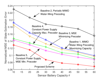
Figure 6: Normalized state estimation error versus battery capacity $\theta$ under $\mathbb{E}\left[\alpha\right]={\normalcolor 40J}$.

VI-B State Estimation MSE Versus Average Energy Arrival $\mathbb{E}\left[\alpha\right]$

Figure 7 illustrates the normalized MSE of the state estimation error versus the average energy arrival $\mathbb{E}\left[\alpha\right]$ with sensor battery capacity $\theta=80J$. It can be observed that the state estimation MSE decreases as the average energy arrival increases. And the proposed scheme has a large performance gain compared with all the baselines.

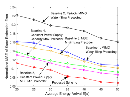
Figure 7: Normalized state estimation error versus average energy arrival $\mathbb{E}\left[\alpha\right]=40J$ under $\theta=80J$.

VII Conclusion

In this paper, we consider an NCS with an energy harvesting sensor that delivers the MIMO dynamic plant state information to a controller over a MIMO fading channel. We derived a low-complexity closed-form dynamic MIMO precoder at the sensor via Lyapunov optimization to stabilize the unstable MIMO dynamic plant. The solution has an event-driven structure and an eigenvalue water-filling structure. We also analyzed the sufficient condition for NCS stability under the proposed MIMO precoder solution. Compared with the various existing MIMO linear precoding schemes, the proposed MIMO precoder solution has substantial state estimation performance gain.

-A Proof of Lemma 1

Denote the history of the realizations of variable $a$ up to time slot $n$ as $a_{0}^{n}\triangleq\cup_{i=1}^{n}\left\{a\left(i\right)\right\}.$ At time slot $n$, the knowledge available to the controller is given by the information set $I_{c}\left(n\right)=\big{\{}\mathbf{u}_{0}^{n-1},\mathbf{\tilde{F}}_{0}^{n},\mathbf{y}_{0}^{n},\gamma_{0}^{n}\big{\}},\ \forall n\in\mathbb{N}^{+}$, with $I_{c}(0)=\big{\{}\tilde{\mathbf{F}}(0),\mathbf{y}(0),\gamma\left(0\right)\big{\}}.$ Let the information set $\widetilde{I}_{c}\left(n\right)=\big{\{}\mathbf{\tilde{F}}_{0}^{n},\mathbf{\tilde{y}}_{0}^{n},\gamma_{0}^{n}\big{\}}$, where $\tilde{\mathbf{y}}(n)=\mathbf{y}\left(n\right)\gamma\left(n\right)$. We define a covariance matrix $\boldsymbol{\Sigma}\left(n\right)=\mathbb{E}\left[\left.\left(\mathbf{x}\left(n\right)-\widetilde{\hat{\mathbf{x}}}\left(n\right)\right)\left(\mathbf{x}\left(n\right)-\widetilde{\hat{\mathbf{x}}}\left(n\right)\right)^{T}\right|\widetilde{I}_{c}\left(n-1\right)\right]$, where $\widetilde{\hat{\mathbf{x}}}\left(n\right)=\mathbb{E}\left[\left.\mathbf{x}\left(n\right)\right|\widetilde{I}_{c}\left(n-1\right)\right]$. Define $\boldsymbol{\Sigma}^{+}\left(n\right)=\mathbb{E}\left[\left.\left(\mathbf{x}\left(n\right)-\widetilde{\hat{\mathbf{x}}}^{+}\left(n\right)\right)\left(\mathbf{x}\left(n\right)-\widetilde{\hat{\mathbf{x}}}^{+}\left(n\right)\right)^{T}\right|\widetilde{I}_{c}\left(n\right)\right]$, where $\widetilde{\hat{\mathbf{x}}}^{+}\left(n\right)=\mathbb{E}\left[\left.\mathbf{x}\left(n\right)\right|\widetilde{I}_{c}\left(n\right)\right]$. Consider a virtual scenario setup where the virtual noisy plant state measurements $\mathbf{y}\left(n\right)=\mathbf{\mathbf{\mathbf{\tilde{F}}}}\left(n\right)\mathbf{x}\left(n\right)+\mathbf{z}\left(n\right)$ are sent across a packet-dropping channel. The packet dropping channel is modeled by $\tilde{\mathbf{y}}(n)=\gamma\left(n\right)\mathbf{y}\left(n\right)$ [12]. This virtual scenario setup coincides with the scenario studied in [28] and by the same argument in [28], the conditional probability density function $p\left(\left.\mathbf{z}\left(n\right)\right|\gamma\left(n\right)\right)$ of $\mathbf{z}\left(n\right)$ is given by: if $\gamma\left(n\right)=1$, $p\left(\left.\mathbf{z}\left(n\right)\right|\gamma\left(n\right)\right)=\mathcal{CN}\left(0,\mathbf{I}\right);$ otherwise, $p\left(\left.\mathbf{z}\left(n\right)\right|\gamma\left(n\right)\right)=\mathcal{CN}\left(0,\sigma\mathbf{I}\right).$ According to the augmented complex Kalman filter algorithm in [29], $\boldsymbol{\Sigma}\left(n+1\right)$ and $\boldsymbol{\Sigma}^{+}\left(n+1\right)$can be obtained recursively as follows [28, 29]:

$$\boldsymbol{\Sigma}\left(n+1\right) =\mathbf{A}\boldsymbol{\Sigma}^{+}\left(n\right)\mathbf{A}^{T}+\mathbf{W};$$ (19)

$$\boldsymbol{\Sigma}^{+}\left(n+1\right) =\boldsymbol{\Sigma}\left(n+1\right)-\boldsymbol{\Sigma}\left(n+1\right)\left(\mathbf{\mathbf{\mathbf{\tilde{F}}}}^{a}\left(n\right)\right)^{H}$$

$$\bigg{(}\mathbf{\mathbf{\mathbf{\tilde{F}}}}^{a}\left(n\right)\boldsymbol{\Sigma}\left(n\right)\big{(}\mathbf{\mathbf{\mathbf{\tilde{F}}}}^{a}\left(n\right)\big{)}^{H}+\gamma\left(n+1\right)\mathbf{I}$$

$$+\left(1-\gamma\left(n+1\right)\right)\sigma\mathbf{I}\bigg{)}^{-1}\mathbf{\mathbf{\mathbf{\tilde{F}}}}^{a}\left(n\right)\boldsymbol{\Sigma}\left(n+1\right)$$ (20)

Combining equation (19) and (20), and taking the limit as $\sigma\rightarrow\infty,$ it follows that the dynamics $\mathbf{\boldsymbol{\Sigma}}\left(n\right)$ is given by equation (7).

Note that given $I_{c}\left(n-1\right)$, $\widetilde{I}_{c}\left(n-1\right)$ is independent of $\mathbf{x}\left(n\right)$. Hence $\mathbf{x}\left(n\right)$, $I_{c}\left(n-1\right)$ and $\widetilde{I}_{c}\left(n-1\right)$ form a Markov chain $\mathbf{x}\left(n\right)\rightarrow I_{c}\left(n-1\right)\rightarrow\widetilde{I}_{c}\left(n-1\right)$ . Hence

$$\mathbb{E}\left[\left.\mathbf{x}\left(n\right)\right|\widetilde{I}_{c}\left(n-1\right)\right]=\mathbb{E}\left[\left.\mathbb{E}\left[\left.\mathbf{x}\left(n\right)\right|I_{c}\left(n-1\right)\right]\right|\widetilde{I}_{c}\left(n-1\right)\right].$$ (21)

By the law of total covariance [30], it follows:

$$\mathrm{Cov}\left[\mathbb{E}\left[\left.\mathbf{x}\left(n\right)\right|I_{c}\left(n-1\right)\right]\right]$$

$$=\mathrm{Cov}\left[\left.\mathbb{E}\left[\left.\mathbf{x}\left(n\right)\right|I_{c}\left(n-1\right)\right]\right|\widetilde{I}_{c}\left(n-1\right)\right]$$

$$+\mathrm{Cov}\left[\mathbb{E}\left[\left.\mathbb{E}\left[\left.\mathbf{x}\left(n\right)\right|I_{c}\left(n-1\right)\right]\right|\widetilde{I}_{c}\left(n-1\right)\right]\right].$$ (22)

Substituting (21) into (22), it follows:

$$\mathrm{Cov}\left[\mathbb{E}\left[\left.\mathbf{x}\left(n\right)\right|I_{c}\left(n-1\right)\right]\right]$$

$$=\mathrm{Cov}\left[\left.\mathbb{E}\left[\left.\mathbf{x}\left(n\right)\right|I_{c}\left(n-1\right)\right]\right|\widetilde{I}_{c}\left(n-1\right)\right]$$

$$+\mathrm{Cov}\left[\mathbb{E}\left[\left.\mathbf{x}\left(n\right)\right|\widetilde{I}_{c}\left(n-1\right)\right]\right].$$ (23)

Furthermore,

$$\mathrm{Cov}\left[\mathbb{E}\left[\left.\mathbf{x}\left(n\right)\right|I_{c}\left(n-1\right)\right]\right]-\mathrm{Cov}\left[\mathbb{E}\left[\left.\mathbf{x}\left(n\right)\right|\widetilde{I}_{c}\left(n-1\right)\right]\right]$$

$$=\mathrm{Cov}\left[\left.\mathbf{x}\left(n\right)\right|\widetilde{I}_{c}\left(n-1\right)\right]-\mathrm{Cov}\left[\left.\mathbf{x}\left(n\right)\right|I_{c}\left(n-1\right)\right].$$ (24)

Substituting (24) into (23), it follows:

$$\mathrm{Cov}\left[\left.\mathbf{x}\left(n\right)\right|I_{c}\left(n-1\right)\right]=\mathrm{Cov}\left[\left.\mathbf{x}\left(n\right)\right|\widetilde{I}_{c}\left(n-1\right)\right]$$

$$-\mathrm{Cov}\left[\left.\mathbb{E}\left[\left.\mathbf{x}\left(n\right)\right|I_{c}\left(n-1\right)\right]\right|\widetilde{I}_{c}\left(n-1\right)\right].$$ (25)

Since covariance matrices are positive semidefinite, it follows:

$$\mathrm{Cov}\left[\left.\mathbf{x}\left(n\right)\right|I_{c}\left(n-1\right)\right] \leq\boldsymbol{\Sigma}\left(n\right).$$ (26)

We construct another Markov chain $\mathbf{x}\left(n\right)\rightarrow I_{c}\left(n\right)\rightarrow I_{c}\left(n-1\right).$ Note that $I_{c}\left(n-1\right)\subseteq I_{c}\left(n\right).$ Therefore, given $I_{c}\left(n\right)$, $I_{c}\left(n-1\right)$ is constant and is independent of $\mathbf{x}\left(n\right)$. Therefore, by definition in Section 2.8 of [21], $\mathbf{x}\left(n\right)$, $I_{c}\left(n\right)$ and $I_{c}\left(n-1\right)$ form a Markov chain $\mathbf{x}\left(n\right)\rightarrow I_{c}\left(n\right)\rightarrow I_{c}\left(n-1\right)$. Applying Proposition 5 in [30], it follows:

$$\mathbb{E}\left[\left.\left(\mathbf{x}\left(n\right)-\hat{\mathbf{x}}\left(n\right)\right)\left(\mathbf{x}\left(n\right)-\hat{\mathbf{x}}\left(n\right)\right)^{T}\right|I_{c}\left(n\right)\right]$$

$$=\mathrm{Var}\left[\left.\mathbf{x}\left(n\right)\right|I_{c}\left(n\right)\right]\leq\mathrm{Var}\left[\left.\mathbf{x}\left(n\right)\right|I_{c}\left(n-1\right)\right]$$

$$=\mathbb{E}\left[\left.\left(\mathbf{x}\left(n\right)-\hat{\mathbf{x}}^{-}\left(n\right)\right)\left(\mathbf{x}\left(n\right)-\hat{\mathbf{x}}^{-}\left(n\right)\right)^{T}\right|I_{c}\left(n-1\right)\right],$$ (27)

where $\hat{\mathbf{x}}^{-}\left(n\right)=\mathbb{E}\left[\left.\mathbf{x}\left(n\right)\right|I_{c}\left(n-1\right)\right]$.

Combining (26) and (27), and taking the trace and expectation w.r.t. $I_{c}\left(n\right)$, it follows the inequality (6). Therefore, Lemma 1 is proved.

-B Proof of Lemma 2

Note that $\mathbf{x}\left(n+1\right)=\mathbf{A}\mathbf{x}\left(n\right)-\mathbf{B}\boldsymbol{\Psi}\mathbf{A}\widetilde{\hat{\mathbf{x}}}\left(n\right)+\mathbf{w}\left(n\right)$, it follows:

$$\left\|\mathbf{x}\left(n+1\right)\right\|^{2} \mathbb{\leq}\left\|\mathbf{A}-\mathbf{B}\boldsymbol{\Psi}\mathbf{A}\right\|^{2}\mathbb{E}\left[\left\|\mathbf{x}\left(n\right)\right\|^{2}\right]$$

$$+\mu_{max}\left(\mathbf{A}\mathbf{A}^{T}\right)\mathbb{E}\left[\left\|\mathbf{x}\left(n\right)-\widetilde{\hat{\mathbf{x}}}\left(n\right)\right\|^{2}\right]+\mathrm{Tr}\left(\mathbf{W}\right).$$ (28)

Since $\mathbf{A}-\mathbf{B}\boldsymbol{\Psi}\mathbf{A}$ is a Hurwitz matrix, then $\left\|\mathbf{A}-\mathbf{B}\boldsymbol{\Psi}\mathbf{A}\right\|<1$. If $\left\|\mathbf{A}-\mathbf{B}\boldsymbol{\Psi}\mathbf{A}\right\|=0$, then $\left\|\mathbf{x}\left(n+1\right)\right\|^{2}<\mu_{max}\left(\mathbf{A}\mathbf{A}^{T}\right)\mathbb{E}\left[\left\|\mathbf{x}\left(n\right)-\widetilde{\hat{\mathbf{x}}}\left(n\right)\right\|^{2}\right]+\mathrm{Tr}\left(\mathbf{W}\right).$ Combining with Lemma 1 and note that $\mathbb{E}\left[\left\|\mathbf{x}\left(n\right)-\widetilde{\hat{\mathbf{x}}}\left(n\right)\right\|^{2}\right]=\mathbb{E}\left[\mathrm{Tr}\left(\boldsymbol{\Sigma}\left(n\right)\right)\right]$, it follows:

$$\underset{N\rightarrow\infty}{\mathrm{limsup}}\frac{1}{N}\sum_{n=1}^{N}\mathbb{E}\left[\left\|\mathbf{x}\left(n+1\right)\right\|^{2}\right]$$

$$<\frac{\mu_{max}\left(\mathbf{A}\mathbf{A}^{T}\right)}{N}\underset{N\rightarrow\infty}{\mathrm{limsup}}\sum_{n=1}^{N}\mathbb{E}\left[\mathrm{Tr}\left(\boldsymbol{\Sigma}\left(n\right)\right)\right]+\mathrm{Tr}\left(\mathbf{W}\right)<\infty.$$ (29)

Similarly, if $\left\|\mathbf{A}-\mathbf{B}\boldsymbol{\Psi}\mathbf{A}\right\|\neq 0$, then

$$\underset{N\rightarrow\infty}{\mathrm{limsup}}\frac{1}{N}\sum_{n=1}^{N}\mathbb{E}\left[\left\|\mathbf{x}\left(n+1\right)\right\|^{2}\right]$$

$$<\frac{\mu_{max}\left(\mathbf{A}\mathbf{A}^{T}\right)}{N\left(1-\left\|\mathbf{A}-\mathbf{B}\boldsymbol{\Psi}\mathbf{A}\right\|\right)}\underset{N\rightarrow\infty}{\mathrm{limsup}}\sum_{n=1}^{N}\mathbb{E}\left[\mathrm{Tr}\left(\boldsymbol{\Sigma}\left(n\right)\right)\right]$$

$$+\frac{\mathrm{Tr}\left(\mathbf{W}\right)}{1-\left\|\mathbf{A}-\mathbf{B}\boldsymbol{\Psi}\mathbf{A}\right\|}<\infty.$$ (30)

Therefore, Lemma 2 is proved.

-C Proof of Lemma 3

By the standard Lyapunov stability theory for discrete-time linear systems, there exist positive definite symmetric matrices $\mathbf{Q}$ and $\mathbf{T}$ such that $\left(\mathbf{A}-\mathbf{B}\mathbf{\Psi}\mathbf{A}\right)^{T}\mathbf{Q}\left(\mathbf{A}-\mathbf{B}\mathbf{\Psi}\mathbf{A}\right)-\mathbf{Q}=-\mathbf{T}$. It follows [31]:

$$\mathbf{x}^{T}\left(n+1\right)\mathbf{S}\mathbf{x}\left(n+1\right)-\mathbf{x}^{T}\left(n\right)\mathbf{S}\mathbf{x}\left(n\right)$$

$$\leq -\mu_{min}\left(\mathbf{T}\right)\left\|\mathbf{x}\left(n\right)\right\|^{2}+2\left\|\mathbf{x}\left(n\right)\right\|\left\|\left(\mathbf{A}-\mathbf{B}\mathbf{\Psi}\mathbf{A}\right)^{T}\mathbf{Q}\right\|$$

$$\cdot\left(\left\|\mathbf{B}\mathbf{\Psi}\mathbf{A}\right\|\left\|\mathbf{x}\left(n\right)-\widetilde{\hat{\mathbf{x}}}\left(n\right)\right\|+\left\|\mathbf{w}\left(n\right)\right\|\right)$$

$$+\left\|\mathbf{Q}\right\|\left(\left\|\mathbf{B}\mathbf{\Psi}\mathbf{A}\right\|\left\|\mathbf{x}\left(n\right)-\widetilde{\hat{\mathbf{x}}}\left(n\right)\right\|+\left\|\mathbf{w}\left(n\right)\right\|\right)^{2}.$$

Define

$$\Theta=\frac{1}{\mu_{min}\left(\mathbf{T}\right)}\bigg{(}\left\|\left(\mathbf{A}-\mathbf{B}\mathbf{\Psi}\mathbf{A}\right)^{T}\mathbf{Q}\right\|$$

$$+\left(\left\|\left(\mathbf{A}-\mathbf{B}\mathbf{\Psi\mathbf{A}}\right)^{T}\mathbf{Q}\right\|^{2}+\mu_{min}\left(\mathbf{T}\right)\left\|\mathbf{Q}\right\|\right)^{\nicefrac{{1}}{{2}}}\bigg{)}\bigg{)},$$

it follows:

• If $\left\|\mathbf{x}\left(n\right)\right\|<\Theta\left(\left\|\mathbf{B}\mathbf{\Psi}\mathbf{A}\right\|\left\|\mathbf{x}\left(n\right)-\widetilde{\hat{\mathbf{x}}}\left(n\right)\right\|+\left\|\mathbf{w}\left(n\right)\right\|\right),$ although the one step drift $\left(\mathbf{x}^{T}\left(n+1\right)\mathbf{Q}\mathbf{x}\left(n+1\right)-\mathbf{x}^{T}\left(n\right)\mathbf{Q}\mathbf{x}\left(n\right)\right)$ is positive, we have

  $$\left\|\mathbf{x}\left(n+1\right)\right\|\leq\left(1+\left\|\mathbf{A}-\mathbf{B}\mathbf{\Psi}\mathbf{A}\right\|\Theta\right)$$

  $$(\left\|\mathbf{B}\mathbf{\Psi}\mathbf{A}\right\|\left\|\mathbf{x}\left(n\right)-\widetilde{\hat{\mathbf{x}}}\left(n\right)\right\|+\left\|\mathbf{w}\left(n\right)\right\|).$$ (31)

• If $\left\|\mathbf{x}\left(n\right)\right\|>\Theta\left(\left\|\mathbf{B}\mathbf{\Psi}\mathbf{A}\right\|\left\|\mathbf{x}\left(n\right)-\widetilde{\hat{\mathbf{x}}}\left(n\right)\right\|+\left\|\mathbf{w}\left(n\right)\right\|\right),$ the one step drift $\mathbf{x}^{T}\left(n+1\right)\mathbf{Q}\mathbf{x}\left(n+1\right)-\mathbf{x}^{T}\left(n\right)\mathbf{Q}\mathbf{x}\left(n\right)$ is negative, hence $\mathbf{x}\left(n+1\right)$ will stay in the ball:

  $$\bigg{\{}\mathbf{x}\left(n+1\right):\left\|\mathbf{x}\left(n+1\right)\right\|\leq\left(1+\left\|\mathbf{A}-\mathbf{B}\mathbf{\Psi}\mathbf{A}\right\|\Theta\right)$$

  $$\left(\left\|\mathbf{B}\mathbf{\Psi}\mathbf{A}\right\|\left\|\mathbf{x}\left(n\right)-\widetilde{\hat{\mathbf{x}}}\left(n\right)\right\|+\left\|\mathbf{w}\left(n\right)\right\|\right)\bigg{\}}.$$

  Hence we have $\left\|\mathbf{x}\left(n\right)\right\|\leq\left(1+\left\|\mathbf{A}-\mathbf{B}\mathbf{\Psi}\right\|\Theta\right)\left(\left\|\mathbf{B}\mathbf{\Psi}\mathbf{A}\right\|\left\|\mathbf{x}\left(n\right)-\widetilde{\hat{\mathbf{x}}}\left(n\right)\right\|+\left\|\mathbf{w}\left(n\right)\right\|\right)$ holds for any time slot $n$.

Note that $\mathrm{Pr}\left[\left.\left\|\mathbf{x}\left(n\right)\right\|^{2}>L^{2}\left(n\right)\right|I_{c}\left(n-1\right)\right]=\mathbb{E}\left[\left.\mathbf{1}\left\{\left\|\mathbf{x}\left(n\right)\right\|^{2}>L^{2}\left(n\right)\right\}\right|I_{c}\left(n-1\right)\right]$. Suppose if $\mathbb{E}\left[\left.\mathbf{1}\left\{\left\|\mathbf{x}\left(n\right)\right\|^{2}>L^{2}\left(n\right)\right\}\right|I_{c}\left(n-1\right)\right]\leq\varepsilon$ holds, then taking expectation on both sides w.r.t. the randomness of $I_{c}\left(n-1\right)$ will yield $\mathbb{E}\left[\mathbf{1}\left\{\left\|\mathbf{x}\left(n\right)\right\|^{2}>L^{2}\left(n\right)\right\}\right]=\mathrm{Pr}\left[\left\|\mathbf{x}\left(n\right)\right\|^{2}>L^{2}\left(n\right)\right]\leq\varepsilon$. Therefore, in order to guarantee the saturation probability of the limiter is at most $\varepsilon$, it is sufficient to design the limiter range $L\left(n\right)$ such that $\mathbb{E}\left[\left.\mathbf{1}\left\{\left\|\mathbf{x}\left(n\right)\right\|^{2}>L^{2}\left(n\right)\right\}\right|I_{c}\left(n-1\right)\right]\leq\varepsilon$ holds for all $n$.

By the Markov’s inequality, it follows:

$$\mathrm{Pr}\left[\left.\left\|\mathbf{x}\left(n\right)\right\|^{2}>L^{2}\left(n\right)\right|I_{c}\left(n-1\right)\right] \leq\frac{\mathbb{E}\left[\left.\left\|\mathbf{x}\left(n\right)\right\|^{2}\right|I_{c}\left(n-1\right)\right]}{L^{2}\left(n\right)}.$$ (32)

Substituting (31) into (32) and applying Lemma (1), it follows:

$$\frac{\mathbb{E}\left[\left.\left\|\mathbf{x}\left(n\right)\right\|^{2}\right|I_{c}\left(n-1\right)\right]}{L^{2}\left(n\right)}$$

$$\leq\frac{1}{L^{2}\left(n\right)}\left(1+\left\|\mathbf{A}-\mathbf{B}\boldsymbol{\Psi}\mathbf{A}\right\|\Theta\right)^{2}$$

$$\cdot\left(\left\|\mathbf{B}\boldsymbol{\Psi}\mathbf{A}\right\|\sqrt{\mathrm{Tr}\left(\boldsymbol{\Sigma}\left(n\right)\right)-\mathrm{Tr}\left(\mathbf{W}\right)}+\sqrt{\mathrm{Tr}\left(\mathbf{W}\right)}\right)^{2}.$$ (33)

Let $\frac{\mathbb{E}\left[\left.\left\|\mathbf{x}\left(n\right)\right\|^{2}\right|I_{c}\left(n-1\right)\right]}{L^{2}\left(n\right)}=\varepsilon,$ we get $L\left(n\right)=\frac{1}{\sqrt{\varepsilon}}\left(1+\left\|\mathbf{A}-\mathbf{B}\boldsymbol{\Psi}\mathbf{A}\right\|\Theta\right)(\left\|\mathbf{B}\boldsymbol{\Psi}\mathbf{A}\right\|\sqrt{\mathrm{Tr}\left(\boldsymbol{\Sigma}\left(n\right)\right)-\mathrm{Tr}\left(\mathbf{W}\right)}+\sqrt{\mathrm{Tr}\left(\mathbf{W}\right)})$, hence Lemma (3) is proved.

-D Proof of Lemma 4

Based on the energy queue dynamics (2), it follows:

$$\mathbb{E}\left\{\left.\frac{1}{2}\left[\left(E\left(n+1\right)-\theta\right)^{2}-\left(E\left(n\right)-\theta\right)^{2}\right]\right|\boldsymbol{\Sigma}\left(n\right)\right\}$$

$$\leq\mathbb{E}\left[\left.\left(\theta-E\left(n\right)\right)M^{2}\mathrm{Tr}\left(\mathbf{F}^{H}(n)\mathbf{F}(n)\right)\tau\right|\boldsymbol{\Sigma}\left(n\right)\right]$$

$$+\mathbb{E}\left[\left(\theta+\alpha\left(n\right)\right)^{2}\right].$$ (34)

Applying Lemma 4 in [32], it follows:

$$\boldsymbol{\Sigma}\left(n\right)\big{(}\mathbf{\mathbf{\mathbf{\tilde{F}}}}^{a}\left(n\right)\big{)}^{H}\Big{(}\mathbf{\mathbf{\mathbf{\tilde{F}}}}^{a}\left(n\right)\boldsymbol{\Sigma}\left(n\right)\big{(}\mathbf{\mathbf{\mathbf{\tilde{F}}}}^{a}\left(n\right)\big{)}^{H}+\mathbf{I}\Big{)}^{-1}\mathbf{\mathbf{\mathbf{\tilde{F}}}}^{a}\left(n\right)\boldsymbol{\Sigma}\left(n\right)$$

$$=\boldsymbol{\Sigma}\left(n\right)-\Big{(}\big{(}\mathbf{\mathbf{\mathbf{\tilde{F}}}}^{a}\left(n\right)\big{)}^{H}\mathbf{\mathbf{\mathbf{\tilde{F}}}}^{a}\left(n\right)+\boldsymbol{\Sigma}\left(n\right)^{-1}\Big{)}^{-1}$$ (35)

Substituting (35) into (7), it follows:

$$\mathbb{E}\left\{\left.\frac{1}{2}\left[\mathrm{Tr}\left(\boldsymbol{\Sigma}\left(n+1\right)\right)-\mathrm{Tr}\left(\boldsymbol{\Sigma}\left(n\right)\right)\right]\right|\boldsymbol{\Sigma}\left(n\right)\right\}$$

$$\leq\frac{1}{2}\mathrm{Tr}(\mathbf{W})+\mathbb{E}\bigg{\{}\frac{\left\|\mathbf{A}\mathbf{A}^{T}\right\|}{2}\bigg{[}\varepsilon\mathrm{Tr}\left(\boldsymbol{\Sigma}\left(n\right)\right)$$

$$+\mathrm{Tr}\bigg{(}2\frac{M^{2}}{L^{2}(n)}\mathrm{Re}\left\{\mathbf{F}^{H}\left(n\right)\mathbf{H}^{H}(n)\mathbf{H}(n)\mathbf{F}\left(n\right)\right\}$$

$$+\boldsymbol{\Sigma}\left(n\right)^{-1}\bigg{)}^{-1}\bigg{]}-\frac{1}{2}\mathrm{Tr}\left(\boldsymbol{\Sigma}\left(n\right)\right)\bigg{|}\boldsymbol{\Sigma}\left(n\right)\bigg{\}}$$ (36)

Adding up (34) and (36) it follows inequality (13), and hence lemma 4 is proved.

-E Proof of Theorem 1

Let $\mathbf{G}(n)=\mathbf{U}^{H}\mathbf{F}\left(n\right),$ denote $\mathbf{G}_{r}(n)=\mathrm{Re}\left\{\mathbf{G}(n)\right\}$ and $\mathbf{G}_{i}(n)=\mathrm{Im}\left\{\mathbf{G}(n)\right\}$. Let $\boldsymbol{\Pi}_{0}=\left[\begin{array}[]{cc}\boldsymbol{\Pi}&\mathbf{0}\\ \mathbf{0}&\boldsymbol{\Pi}\end{array}\right]$, $\widetilde{\mathbf{G}}\left(n\right)=\left[\begin{array}[]{c}\mathbf{G}_{r}(n)\\ \mathbf{G}_{i}(n)\end{array}\right]$. Define $f\left(\widetilde{\mathbf{G}}\right)=\frac{\left\|\mathbf{A}\mathbf{A}^{T}\right\|}{2}\mathrm{Tr}\left(2\widetilde{\mathbf{G}}^{T}\boldsymbol{\Pi}_{0}\widetilde{\mathbf{G}}+\boldsymbol{\Sigma}^{-1}\right)^{-1}+M^{2}\tau\left(\theta-E\right)\mathrm{Tr}\left(\widetilde{\mathbf{G}}^{T}\widetilde{\mathbf{G}}\right).$ For any given $\widetilde{\mathbf{G}}$, there is a decomposition that $\widetilde{\mathbf{G}}=\widetilde{\mathbf{G}}_{1}+\widetilde{\mathbf{G}}_{2}$, where $\mathrm{col}\left(\widetilde{\mathbf{G}}_{1}\right)\subseteq\mathrm{span}\left(\mathrm{col}\left(\boldsymbol{\Pi}_{0}\right)\right)$ and $\mathrm{col}\left(\widetilde{\mathbf{G}}_{2}\right)\subseteq\mathrm{span}\left(\mathrm{col}\left(\boldsymbol{\Pi}_{0}\right)\right)^{\perp}$, and we have $f\left(\widetilde{\mathbf{G}}_{1}\right)\leq f\left(\widetilde{\mathbf{G}}\right)$. Therefore, $\mathbf{G}^{\ast}(n)$ must satisfy $\mathrm{col}\left(\widetilde{\mathbf{G}}^{\ast}\left(n\right)\right)\subseteq\mathrm{span}\left(\mathrm{col}\left(\boldsymbol{\Pi}_{0}\right)\right)$, i.e., $\mathrm{col}\left(\mathbf{F}^{\ast}\left(n\right)\right)\subseteq\mathrm{span}\left(\mathrm{col}\left(\mathbf{H}\right)\right)$. Let $\boldsymbol{\widetilde{\Delta}}_{1}=\left[\begin{array}[]{cc}\boldsymbol{\Delta}_{1}&\mathbf{0}\\ \mathbf{0}&\boldsymbol{\Delta}_{1}\end{array}\right]$ where $\boldsymbol{\Delta}_{1}=\left[\begin{array}[]{cc}\widetilde{\boldsymbol{\Pi}}&\mathbf{0}\\ \mathbf{0}&\mathbf{0}\end{array}\right]$ and $\widetilde{\boldsymbol{\Pi}}$ is the leading principal minor of order $\mathrm{min}\left(N_{s},N_{t}\right)$ of $\boldsymbol{\Pi}$. Let $\boldsymbol{\widetilde{\Delta}}_{2}=\left[\begin{array}[]{cc}\boldsymbol{\Delta}_{2}&\mathbf{0}\\ \mathbf{0}&\boldsymbol{\Delta}_{2}\end{array}\right]$ where $\boldsymbol{\Delta}_{2}=\left[\begin{array}[]{cc}\widetilde{\boldsymbol{\Pi}}^{-1}&\mathbf{0}\\ \mathbf{0}&\mathbf{0}\end{array}\right]$. Let $\widetilde{\mathbf{S}}=\left[\begin{array}[]{cc}\hat{\mathbf{S}}&\mathbf{0}\\ \mathbf{0}&\hat{\mathbf{S}}\end{array}\right]$, where $\hat{\mathbf{S}}=\left[\begin{array}[]{cc}\mathbf{S}&\mathbf{0}\\ \mathbf{0}&\mathbf{I}_{\left(N_{t}-K\right)\times\left(N_{t}-K\right)}\end{array}\right]$. Let $\mathbf{X}(n)=\frac{M}{L(\boldsymbol{\Sigma})}\widetilde{\mathbf{S}}\boldsymbol{\Delta}_{1}\widetilde{\mathbf{G}}\left(n\right)$. Then Problem 1 is transformed into the following problem:

$$\mathcal{P}_{1}:\underset{\mathrm{\mathbf{X}}\left(n\right)}{\mathrm{min}} \ \ L^{2}(\boldsymbol{\Sigma})\mathrm{Tr}\left(\widetilde{\mathbf{S}}\boldsymbol{\widetilde{\Delta}}_{2}^{2}\widetilde{\mathbf{S}}^{T}\mathbf{X}(n)\mathbf{X}^{T}(n)\right)\tau\left(\theta-E\right)$$

$$+\frac{\left\|\mathbf{A}\mathbf{A}^{T}\right\|}{2}\mathrm{Tr}\left(2\mathbf{X}^{T}(n)\mathbf{X}(n)+\boldsymbol{\Sigma}^{-1}\right)^{-1}$$

$$s.t. \ \ L^{2}(\boldsymbol{\Sigma})\mathrm{Tr}\left(\widetilde{\mathbf{S}}\boldsymbol{\widetilde{\Delta}}_{2}^{2}\widetilde{\mathbf{S}}^{T}\mathbf{X}(n)\mathbf{X}^{T}(n)\right)\tau\leq E.$$

The associated KKT conditions are given by

$$L^{2}(\boldsymbol{\Sigma})\mathrm{Tr}\left(\widetilde{\mathbf{S}}\boldsymbol{\widetilde{\Delta}}_{2}^{2}\widetilde{\mathbf{S}}^{T}\mathbf{X}^{\ast}(n)\left(\mathbf{X}^{\ast}(n)\right)^{T}\right)\tau-E\leq 0;$$ (37)

$$\beta\geq 0;$$ (38)

$$\beta\left[L^{2}(\boldsymbol{\Sigma})\mathrm{Tr}\left(\widetilde{\mathbf{S}}\boldsymbol{\widetilde{\Delta}}_{2}^{2}\widetilde{\mathbf{S}}^{T}\mathbf{X}(n)\mathbf{X}^{T}(n)\right)\tau-E\right]=0;$$ (39)

$$\left\|\mathbf{A}\mathbf{A}^{T}\right\|\mathbf{X}(n)\left(2\mathbf{X}^{T}(n)\mathbf{X}(n)+\boldsymbol{\Sigma}^{-1}\right)^{-2}$$

$$+\left(\theta-E+\beta\right)\tau L^{2}(\boldsymbol{\Sigma})\widetilde{\mathbf{S}}\boldsymbol{\widetilde{\Delta}}_{2}^{2}\widetilde{\mathbf{S}}^{T}\mathbf{X}(n)=\mathbf{0}.$$ (40)

Note that for non-convex problems, the KKT condition is necessary and in order to find the global optimum, we need to test all the solutions that satisfy the KKT conditions. Therefore, without loss of optimality, we restrict the feasible solution set of the optimization problem to be the solutions that satisfy the KKT conditions (37)- (40). By exploiting the structural properties of the solutions that satisfy the of the KKT conditions, the objective function of the optimization problem can be further simplified. Let $\widetilde{\mathbf{X}}(n)=\widetilde{\mathbf{S}}^{T}\mathbf{X}(n)\mathbf{S}$, the KKT condition (37)- (40) are equivalent to the following conditions (41)- (44).

$$L^{2}(\boldsymbol{\Sigma})\mathrm{Tr}\left(\boldsymbol{\widetilde{\Delta}}_{2}^{2}\widetilde{\mathbf{X}}(n)\widetilde{\mathbf{X}}^{T}(n)\right)\tau-E\leq 0;$$ (41)

$$\beta\geq 0;$$ (42)

$$\beta\left[L^{2}(\boldsymbol{\Sigma})\mathrm{Tr}\left(\boldsymbol{\widetilde{\Delta}}_{2}^{2}\widetilde{\mathbf{X}}^{T}(n)\widetilde{\mathbf{X}}(n)\right)\tau-E\right]=0;$$ (43)

$$\left(2\widetilde{\mathbf{X}}^{T}(n)\widetilde{\mathbf{X}}(n)+\boldsymbol{\Lambda}^{-1}\right)^{-2}\widetilde{\mathbf{X}}^{T}(n)$$

$$=\frac{\left(\theta-E+\beta\right)\tau L^{2}(\boldsymbol{\Sigma})}{\left\|\mathbf{A}\mathbf{A}^{T}\right\|}\widetilde{\mathbf{X}}^{T}(n)\boldsymbol{\widetilde{\Delta}}_{2}^{2}.$$ (44)

It follows that every column of $\widetilde{\mathbf{X}}^{T}(n)$ that corresponds to a nonzero diagonal element of $\boldsymbol{\widetilde{\Delta}}_{2}^{2}$ is an eigenvector of $\left(2\widetilde{\mathbf{X}}^{T}(n)\widetilde{\mathbf{X}}(n)+\boldsymbol{\Lambda}^{-1}\right)^{-2}$. Hence, it follows

$$\left(2\widetilde{\mathbf{X}}^{T}(n)\widetilde{\mathbf{X}}(n)+\boldsymbol{\Lambda}^{-1}\right)\widetilde{\mathbf{X}}^{T}(n)\widetilde{\mathbf{X}}(n)$$

$$=\sqrt{\frac{\left\|\mathbf{A}\mathbf{A}^{T}\right\|}{\left(\theta-E+\beta\right)\tau L^{2}(\boldsymbol{\Sigma})}}\widetilde{\mathbf{X}}^{T}(n))\boldsymbol{\widetilde{\Delta}}_{1}\widetilde{\mathbf{X}}(n).$$ (45)

Since $\widetilde{\mathbf{X}}^{T}(n))\boldsymbol{\widetilde{\Delta}}_{1}\widetilde{\mathbf{X}}(n)$ is symmetric matrices, it follows $\left(2\widetilde{\mathbf{X}}^{T}(n)\widetilde{\mathbf{X}}(n)+\boldsymbol{\Lambda}^{-1}\right)$ and $\widetilde{\mathbf{X}}^{T}(n)\widetilde{\mathbf{X}}(n)$ commute, and $\widetilde{\mathbf{X}}^{T}(n)\widetilde{\mathbf{X}}(n)$ and $\boldsymbol{\Lambda}^{-1}$ commute. Therefore, $\widetilde{\mathbf{X}}^{T}(n)\widetilde{\mathbf{X}}(n)$ and $\boldsymbol{\Lambda}^{-1}$ are simultaneous diagonalizable, i.e., there exist an unitary matrix $\mathbf{P}$, such that $\widetilde{\mathbf{X}}^{T}(n)\widetilde{\mathbf{X}}(n)=\mathbf{P}\mathrm{diag}\left(\sigma_{1},\ldots,\sigma_{K}\right)\mathbf{P}^{T},$ and $\boldsymbol{\Lambda}^{-1}=\mathrm{diag}\left(\lambda_{1},\ldots,\lambda_{K}\right)$, where $\sigma_{1},\ldots,\sigma_{K}$ and $\lambda_{1},\ldots,\lambda_{K}$ are the eigenvalues of $\widetilde{\mathbf{X}}^{T}(n)\widetilde{\mathbf{X}}(n)$ and $\boldsymbol{\Lambda}^{-1}$, respectively. Hence, it follows the value of the objective function of Problem $\mathcal{P}_{1}$ is given by:

$$L^{2}(\boldsymbol{\Sigma})\mathrm{Tr}\left(\widetilde{\mathbf{S}}\boldsymbol{\widetilde{\Delta}}_{2}^{2}\widetilde{\mathbf{S}}^{T}\mathbf{X}(n)\mathbf{X}^{T}(n)\right)\tau\left(\theta-E\right)$$

$$+\frac{\left\|\mathbf{A}\mathbf{A}^{T}\right\|}{2}\mathrm{Tr}\left(2\mathbf{X}^{T}(n)\mathbf{X}(n)+\boldsymbol{\Sigma}^{-1}\right)^{-1}$$

$$= \left\|\mathbf{A}\mathbf{A}^{T}\right\|\sum_{i=1}^{K}\left[\left(2\sigma_{i}+\lambda_{i}\right)^{-2}\sigma_{i}\right]+\frac{\left\|\mathbf{A}\mathbf{A}^{T}\right\|}{2}\sum_{i=1}^{K}\left(2\sigma_{i}+\lambda_{i}\right)^{-1}.$$ (46)

Note the optimal solution $\widetilde{\mathbf{X}}(n)$ must satisfy the KKT condition (41)-(44). However, (46) implies that for any $\widetilde{\mathbf{X}}(n)$ satisfies the KKT condition (41)-(44), the value of the objective function of of Problem $\mathcal{P}_{1}$ only depends on the eigenvalues of $\widetilde{\mathbf{X}}^{T}(n)\widetilde{\mathbf{X}}(n)$, i.e., $\sigma_{1},\ldots,\sigma_{K},$ and independent of the structure of $\widetilde{\mathbf{X}}(n)$. Hence, let $\widetilde{\mathbf{X}}(n)=\left[\begin{array}[]{c}\widehat{\mathbf{X}}(n)\\ \mathbf{0}\end{array}\right]$, where $\widehat{\mathbf{X}}(n)\in\mathbb{R}^{K\times K}$ is a diagonal matrix, and let $\mathbf{Y}\left(n\right)=\widehat{\mathbf{X}}^{T}(n)\widehat{\mathbf{X}}(n)$. And Problem $\mathcal{P}_{1}$ is equivalent to the following Problem $\mathcal{P}_{2}:$

$$\mathcal{P}_{2}:\underset{\mathbf{Y}\left(n\right)}{\mathrm{min}} \ \ L^{2}(\boldsymbol{\Sigma})\mathrm{Tr}\left(\boldsymbol{\Pi}_{K}^{-2}\mathbf{Y}\left(n\right)\right)\tau\left(\theta-E\right)$$

$$+\frac{\left\|\mathbf{A}\mathbf{A}^{T}\right\|}{2}\mathrm{Tr}\left(2\mathbf{Y}\left(n\right)+\boldsymbol{\Lambda}^{-1}\right)^{-1}$$

$$s.t. \ \ L^{2}(\boldsymbol{\Sigma})\mathrm{Tr}\left(\boldsymbol{\Pi}_{K}^{-2}\mathbf{Y}\left(n\right)\right)\tau\leq E.$$

Note that $\mathrm{Tr}\left(\boldsymbol{\Pi}_{K}^{-2}\mathbf{Y}\left(n\right)\right)$ is convex in $\mathbf{Y}\left(n\right)$, $\mathrm{Tr}\left(2\mathbf{Y}\left(n\right)+\boldsymbol{\Lambda}^{-1}\right)^{-1}$ is convex in $\mathbf{Y}\left(n\right)$. Hence the objective function $L(\boldsymbol{\Sigma})\mathrm{Tr}\left(\boldsymbol{\Pi}_{K}^{-2}\mathbf{Y}\left(n\right)\right)\tau\left(\theta-E\right)+\frac{\left\|\mathbf{A}\mathbf{A}^{T}\right\|}{2}\mathrm{Tr}\left(2\mathbf{Y}\left(n\right)+\boldsymbol{\Lambda}^{-1}\right)^{-1}$ of Problem $\mathcal{P}_{2}$ is convex in $\mathbf{Y}\left(n\right)$. The constraint of Problem $\mathcal{P}_{2}$ is also convex in $\mathbf{Y}\left(n\right).$ Therefore, Problem $\mathcal{P}_{2}$ is convex. Therefore, we conclude that Problem 1 is equivalent to Problem $\mathcal{P}_{2}$ which is a convex optimization problem. The optimal solution $\mathbf{Y}^{\ast}\left(n\right)$ is given by

$$\mathbf{Y}^{\ast}\left(n\right) =\frac{1}{2}\left[\frac{\boldsymbol{\Pi}_{K}}{L\left(\boldsymbol{\Sigma}\right)}\sqrt{\frac{\left\|\mathbf{A}\mathbf{A}^{T}\right\|}{\left(\left[\theta-E\right]^{+}+\beta\right)\tau}}-\boldsymbol{\Lambda}^{-1}\right]^{+},$$ (47)

where $\beta=0$ if $L^{2}(\boldsymbol{\Sigma})\mathrm{Tr}\left(\boldsymbol{\Pi}_{K}^{-2}\mathbf{Y}^{*}\left(n\right)\right)\tau<E$, else $\beta$ is chosen such that $L^{2}(\boldsymbol{\Sigma})\mathrm{Tr}\left(\boldsymbol{\Pi}_{K}^{-2}\mathbf{Y}^{*}\left(n\right)\right)\tau=E$. Since $\widehat{\mathbf{X}^{\ast}}(n)=\left(\mathbf{Y}^{\ast}\left(n\right)\right)^{\frac{1}{2}},$ $\widetilde{\mathbf{X}}(n)=\left[\begin{array}[]{c}\widehat{\mathbf{X}}(n)\\ \mathbf{0}\end{array}\right]$ and $\mathbf{X}(n)=\widetilde{\mathbf{S}}\widetilde{\mathbf{X}}(n)\mathbf{S}^{T}$, it follows $\mathbf{X}^{\ast}(n)=\left[\begin{array}[]{c}\mathbf{S}\widetilde{\boldsymbol{\Lambda}}\mathbf{S}^{T}\\ \mathbf{0}\end{array}\right],$ where

$$\widetilde{\boldsymbol{\Lambda}}=\Big{(}\frac{1}{2}\Big{[}\frac{\boldsymbol{\Pi}_{K}}{L\left(\boldsymbol{\Sigma}\right)}\sqrt{\frac{\left\|\mathbf{A}\mathbf{A}^{T}\right\|}{\left(\left[\theta-E\right]^{+}+\beta\right)\tau}}-\boldsymbol{\Lambda}^{-1}\Big{]}^{+}\Big{)}^{\nicefrac{{1}}{{2}}}.$$ (48)

Therefore, $\mathbf{F}^{\ast}\left(n\right)=\frac{L(\boldsymbol{\Sigma})}{M}\mathbf{U}\left[\begin{array}[]{c}\boldsymbol{\Pi}_{K}^{-1}\widetilde{\boldsymbol{\Lambda}}\mathbf{S}^{T}\\ \mathbf{0}\end{array}\right]$, and if $L^{2}(\boldsymbol{\Sigma})\mathrm{Tr}\Big{(}\frac{1}{2}\boldsymbol{\Pi}_{K}^{-2}\Big{[}\frac{\boldsymbol{\Pi}_{K}}{L\left(\boldsymbol{\Sigma}\right)}\sqrt{\frac{\left\|\mathbf{A}\mathbf{A}^{T}\right\|}{\left(\theta-E\right)\tau}}\mathbf{I}-\boldsymbol{\Lambda}^{-1}\Big{]}^{+}\Big{)}\tau<E$ then $\beta=0$, else $\beta$ is chosen such that $M^{2}\mathrm{Tr}\left(\left(\mathbf{F}^{\ast}(n)\right)^{H}\mathbf{F}^{\ast}(n)\right)\tau=E$. Therefore, Theorem is 1 proved.

-F Proof of Theorem 2

Intuitively, the negative Lyapunov drift is related to the stability of the MIMO plant. Therefore, the sufficient condition for stability should be the sufficient condition to guarantee negative Lyapunov drift. Substituting the MIMO precoding solution in Theorem 1 into (36), it follows:

$$\mathrm{Tr}\left(2\frac{M^{2}}{L^{2}(n)}\mathrm{Re}\left\{\mathbf{F}^{H}\left(n\right)\mathbf{H}^{H}(n)\mathbf{H}(n)\mathbf{F}\left(n\right)\right\}+\boldsymbol{\Sigma}\left(n\right)^{-1}\right)^{-1}$$

$$= \mathrm{Tr}\left(\left[\frac{\boldsymbol{\Pi}_{K}}{L\left(\boldsymbol{\Sigma}\right)}\sqrt{\frac{\left\|\mathbf{A}\mathbf{A}^{T}\right\|}{\left(\left[\theta-E\right]^{+}+\beta\right)\tau}}-\boldsymbol{\Lambda}^{-1}\right]^{+}+\boldsymbol{\Lambda}^{-1}\right)^{-1}$$

$$\leq \mathrm{Tr}\left(\left[\frac{\boldsymbol{\Pi}_{K}E}{\mathrm{Tr}\left(\boldsymbol{\Pi}_{K}^{-1}\right)\tau L^{2}\left(\boldsymbol{\Sigma}\right)\mathcal{M}\left(\mathbf{A}\right)}-\lambda_{min}\mathbf{I}\right]^{+}+\lambda_{min}\mathbf{I}\right)^{-1}$$

$$+\frac{\theta^{2}}{\left\|\mathbf{A}\mathbf{A}^{T}\right\|}$$

$$= K\mathrm{min}\left\{\tilde{\pi}^{-1}\frac{\tau L^{2}\left(\boldsymbol{\Sigma}\right)\mathcal{M}\left(\mathbf{A}\right)}{E},\lambda_{min}^{-1}\right\}+\frac{\theta^{2}}{\left\|\mathbf{A}\mathbf{A}^{T}\right\|},$$ (49)

where $\tilde{\pi}=\frac{\pi}{\mathrm{Tr}\left(\boldsymbol{\Pi}_{K}^{-1}\right)}$ and $\pi$ is the unordered singular value of $\mathbf{H}$ and $\lambda_{min}$ is the minimum nonzero element of $\boldsymbol{\Lambda}^{-1}$. Furthermore,

$$\mathbb{E}\left[\left.K\mathrm{min}\left\{\tilde{\pi}^{-1}\frac{\tau L^{2}\left(\boldsymbol{\Sigma}\right)\mathcal{M}\left(\mathbf{A}\right)}{E},\lambda_{min}^{-1}\right\}\right|\boldsymbol{\Sigma}\left(n\right)\right]$$

$$\leq \mathbb{E}\left[\left.K\mathrm{min}\left\{\tilde{\pi}^{-1}\frac{\tau L^{2}\left(\boldsymbol{\Sigma}\right)\mathcal{M}\left(\mathbf{A}\right)}{E},\mathrm{Tr}\left(\boldsymbol{\Sigma}\left(n\right)\right)\right\}\right|\boldsymbol{\Sigma}\left(n\right)\right],$$

where the expectation is taken w.r.t. the randomness of $\tilde{\pi}$ and $E$. Note that $\tilde{\pi}$ is independent of $\boldsymbol{\Sigma}\left(n\right)$ and $\alpha\left(n\right)$, and there exists a constant $\xi$ such that

$$\mathbb{E}_{\tilde{\pi},E}\left[\left.K\mathrm{min}\left\{\tilde{\pi}^{-1}\frac{\tau L^{2}\left(\boldsymbol{\Sigma}\right)\mathcal{M}\left(\mathbf{A}\right)}{E},\mathrm{Tr}\left(\boldsymbol{\Sigma}\left(n\right)\right)\right\}\right|\boldsymbol{\Sigma}\left(n\right)\right]$$

$$\leq K\mathrm{Pr}\left(\tilde{\pi}<\xi\right)\mathrm{Tr}\left(\boldsymbol{\Sigma}\left(n\right)\right)$$

$$+K\tau L^{2}\left(\boldsymbol{\Sigma}\right)\mathcal{M}\left(\mathbf{A}\right)\mathbb{E}\left[\left.\tilde{\pi}^{-1}\right|\tilde{\pi}\geq\xi\right]\mathbb{E}\left[\left.\frac{1}{E}\right|\boldsymbol{\Sigma}\left(n\right)\right]$$ (50)

Furthermore, let $\delta=\sqrt{\frac{2}{\varepsilon}}\left(1+\left\|\mathbf{A}-\mathbf{B}\boldsymbol{\Psi}\mathbf{A}\right\|\Theta\right)\left\|\mathbf{B}\boldsymbol{\Psi}\right\|\left\|\mathbf{A}\right\|$, it follows:

$$L^{2}\left(n\right)\leq\frac{1}{\varepsilon}\left(1+\left\|\mathbf{A}-\mathbf{B}\boldsymbol{\Psi}\mathbf{A}\right\|\Theta\right)^{2}$$

$$\cdot(\left\|\mathbf{B}\boldsymbol{\Psi}\mathbf{A}\right\|\sqrt{\mathrm{Tr}\left(\boldsymbol{\Sigma}\left(n\right)\right)}+\sqrt{\mathrm{Tr}\left(\mathbf{W}\right)})^{2}$$

$$\leq\frac{\delta^{2}}{\left\|\mathbf{B}\boldsymbol{\Psi}\right\|^{2}\left\|\mathbf{A}\right\|^{2}}\left(\left\|\mathbf{B}\boldsymbol{\Psi}\mathbf{A}\right\|^{2}\mathrm{Tr}\left(\boldsymbol{\Sigma}\left(n\right)\right)+\mathrm{Tr}\left(\mathbf{W}\right)\right)$$ (51)

Note that if $\left[E\left(n-1\right)-\|\mathbf{F}\left(n-1\right)\mathbf{q}\left(n-1\right)\|^{2}\tau\right]^{+}+\alpha\left(n-1\right)<\theta$, then $E>\alpha\left(n-1\right)$. Since $\alpha\left(n\right)$ is i.i.d. energy arrival and independent of $\boldsymbol{\Sigma}\left(n\right)$, it follows $\mathbb{E}\left[\left.\frac{1}{E}\right|\boldsymbol{\Sigma}\left(n\right)\right]<\mathbb{E}\left[\frac{1}{\alpha}\right]$. If $\left[E\left(n-1\right)-\|\mathbf{F}\left(n-1\right)\mathbf{q}\left(n-1\right)\|^{2}\tau\right]^{+}+\alpha\left(n-1\right)\geq\theta$, then $E=\theta$ and $\mathbb{E}\left[\left.\frac{1}{E}\right|\boldsymbol{\Sigma}\left(n\right)\right]=\frac{1}{\theta}$. Therefore $\mathbb{E}\left[\left.\frac{1}{E}\right|\boldsymbol{\Sigma}\left(n\right)\right]\leq\mathrm{Pr}([E\left(n-1\right)-\|\mathbf{F}\left(n-1\right)\mathbf{q}\left(n-1\right)\|^{2}\tau]^{+}+\alpha\left(n-1\right)<\theta|\boldsymbol{\Sigma}\left(n\right))\mathbb{E}\left[\frac{1}{\alpha}\right]+\mathrm{Pr}([E\left(n-1\right)-\|\mathbf{F}\left(n-1\right)\mathbf{q}\left(n-1\right)\|^{2}\tau]^{+}+\alpha\left(n-1\right)\geq\theta|\boldsymbol{\Sigma}\left(n\right))\frac{1}{\theta}<\mathbb{E}\left[\frac{1}{\alpha}\right]+\frac{1}{\theta}$. Substituting (49), (50) and (51) into the drift of $\boldsymbol{\Sigma}\left(n\right)$ (36), it follows:

$$\mathbb{E}\left\{\left.\left[\mathrm{Tr}\left(\boldsymbol{\Sigma}\left(n+1\right)\right)-\mathrm{Tr}\left(\boldsymbol{\Sigma}\left(n\right)\right)\right]\right|\boldsymbol{\Sigma}\left(n\right)\right\}$$

$$\leq\bigg{(}1+K\tau\frac{\delta^{2}}{\left\|\mathbf{B}\boldsymbol{\Psi}\right\|^{2}}\mathcal{M}\left(\mathbf{A}\mathbf{A}^{T}\right)\mathcal{M}\left(\mathbf{A}\right)\mathbb{E}\left[\left.\tilde{\pi}^{-1}\right|\tilde{\pi}\geq\xi\right]$$

$$\cdot\left(\mathbb{E}\left[\frac{1}{\alpha}\right]+\frac{1}{\theta}\right)\bigg{)}\mathrm{Tr}\left(\mathbf{W}\right)+\theta^{2}+\mathrm{Tr}\left(\boldsymbol{\Sigma}\left(n\right)\right)\bigg{\{}\varepsilon\mathcal{M}\left(\mathbf{A}\mathbf{A}^{T}\right)$$

$$+K\mathrm{Pr}\left(\tilde{\pi}<\xi\right)\mathcal{M}\left(\mathbf{A}\mathbf{A}^{T}\right)+\delta^{2}K\left(\mathbb{E}\left[\frac{1}{\alpha}\right]+\frac{1}{\theta}\right)\tau$$

$$\cdot\mathcal{M}\left(\mathbf{A}\mathbf{A}^{T}\right)\mathcal{M}\left(\mathbf{A}\right)\mathbb{E}\left[\left.\tilde{\pi}^{-1}\right|\tilde{\pi}\geq\xi\right]-1\bigg{\}}.$$ (52)

Therefore, a sufficient condition for stability is given by $\varepsilon\mathcal{M}\left(\mathbf{A}\mathbf{A}^{T}\right)+K\mathrm{Pr}\left(\tilde{\pi}<\xi\right)\mathcal{M}\left(\mathbf{A}\mathbf{A}^{T}\right)+\delta^{2}K\left(\mathbb{E}\left[\frac{1}{\alpha}\right]+\frac{1}{\theta}\right)\tau\mathcal{M}\left(\mathbf{A}\mathbf{A}^{T}\right)\mathcal{M}\left(\mathbf{A}\right)\mathbb{E}\left[\left.\tilde{\pi}^{-1}\right|\tilde{\pi}\geq\xi\right]-1<0,$ i.e.,

$$\mathbb{E}\left[\frac{1}{\alpha}\right]+\frac{1}{\theta}<\frac{1-\left(\varepsilon+K\mathrm{Pr}\left(\tilde{\pi}<\xi\right)\right)\mathcal{M}\left(\mathbf{A}\mathbf{A}^{T}\right)}{\delta^{2}K\tau\mathbb{E}\left[\left.\tilde{\pi}^{-1}\right|\tilde{\pi}\geq\xi\right]\mathcal{M}\left(\mathbf{A}\right)\mathcal{M}\left(\mathbf{A}\mathbf{A}^{T}\right)}.$$ (53)

Since there exists a constant $\xi$ such that (50) holds, and for that typical $\xi$ there is a sufficient condition in the form of (53) . Therefore, $\xi$ is chosen as $\xi^{\ast}=\underset{\xi}{\mathrm{arg}\ \mathrm{max}}\ \frac{1-\left(\varepsilon+K\mathrm{Pr}\left(\tilde{\pi}<\xi\right)\right)\mathcal{M}\left(\mathbf{A}\mathbf{A}^{T}\right)}{K\delta^{2}\tau\mathbb{E}\left[\left.\tilde{\pi}^{-1}\right|\tilde{\pi}\geq\xi\right]\mathcal{M}\left(\mathbf{A}\right)\mathcal{M}\left(\mathbf{A}\mathbf{A}^{T}\right)}$, and hence Theorem 2 is proved.

-G Proof of Theorem 3

If the sufficient condition of stability (16) is satisfied, then denote a positive constant $\eta$ as $\eta=1-(\varepsilon+K\mathrm{Pr}\left(\tilde{\pi}<\xi^{\ast}\right))\mathcal{M}\left(\mathbf{A}\mathbf{A}^{T}\right)-\left(\mathbb{E}\left[\frac{1}{\alpha}\right]+\frac{1}{\theta}\right)KT\delta^{2}\tau\mathbb{E}\left[\left.\tilde{\pi}^{-1}\right|\tilde{\pi}\geq\xi^{\ast}\right]\mathcal{M}\left(\mathbf{A}\right)\mathcal{M}\left(\mathbf{A}\mathbf{A}^{T}\right).$ Substituting $\eta$ into equation (52), it follows:

$$\mathbb{E}\left\{\left.\left[\mathrm{Tr}\left(\boldsymbol{\Sigma}\left(n+1\right)\right)-\mathrm{Tr}\left(\boldsymbol{\Sigma}\left(n\right)\right)\right]\right|\boldsymbol{\Sigma}\left(n\right)\right\}$$

$$\leq (1+K\tau\frac{\delta^{2}}{\left\|\mathbf{B}\boldsymbol{\Psi}\right\|^{2}}\mathcal{M}\left(\mathbf{A}\right)\mathcal{M}\left(\mathbf{A}\mathbf{A}^{T}\right)\mathbb{E}\left[\left.\tilde{\pi}^{-1}\right|\tilde{\pi}\geq\xi\right]$$

$$\cdot\left(\mathbb{E}\left[\frac{1}{\alpha}\right]+\frac{1}{\theta}\right))\mathrm{Tr}\left(\mathbf{W}\right)+\theta^{2}-\eta\mathrm{Tr}\left(\boldsymbol{\Sigma}\left(n\right)\right).$$ (54)

Taking expectation w.r.t. $\boldsymbol{\Sigma}\left(n\right)$ at both side of (54) and using the law of iterated expectations yields:

$$\mathbb{E}\left[\mathrm{Tr}\left(\boldsymbol{\Sigma}\left(n+1\right)\right)-\mathrm{Tr}\left(\boldsymbol{\Sigma}\left(n\right)\right)\right]$$

$$\leq (1+K\tau\frac{\delta^{2}}{\left\|\mathbf{B}\boldsymbol{\Psi}\right\|^{2}}\mathcal{M}\left(\mathbf{A}\right)\mathcal{M}\left(\mathbf{A}\mathbf{A}^{T}\right)\mathbb{E}\left[\left.\tilde{\pi}^{-1}\right|\tilde{\pi}\geq\xi\right]$$

$$\cdot\left(\mathbb{E}\left[\frac{1}{\alpha}\right]+\frac{1}{\theta}\right))\mathrm{Tr}\left(\mathbf{W}\right)+\theta^{2}-\eta\mathbb{E}\left[\mathrm{Tr}\left(\boldsymbol{\Sigma}\left(n\right)\right)\right].$$ (55)

Summing over time sots $n\in\left\{0,\ldots,N-1\right\}$ and dividing by $N$ yields

$$\frac{\mathbb{E}\left[\mathrm{Tr}\left(\boldsymbol{\Sigma}\left(N\right)\right)-\mathrm{Tr}\left(\boldsymbol{\Sigma}\left(0\right)\right)\right]}{N}$$

$$\leq(1+K\tau\frac{\delta^{2}}{\left\|\mathbf{B}\boldsymbol{\Psi}\right\|^{2}}\mathcal{M}\left(\mathbf{A}\right)\mathcal{M}\left(\mathbf{A}\mathbf{A}^{T}\right)\mathbb{E}\left[\left.\tilde{\pi}^{-1}\right|\tilde{\pi}\geq\xi\right]$$

$$\cdot\left(\mathbb{E}\left[\frac{1}{\alpha}\right]+\frac{1}{\theta}\right))\mathrm{Tr}\left(\mathbf{W}\right)+\theta^{2}-\frac{\eta}{N}\sum_{n=0}^{N-1}\mathbb{E}\left[\mathrm{Tr}\left(\boldsymbol{\Sigma}\left(n\right)\right)\right].$$ (56)

By non-negativity of $\mathrm{Tr}\left(\boldsymbol{\Sigma}\left(n\right)\right)$, it follows:

$$\frac{1}{N}\sum_{n=0}^{N-1}\mathbb{E}\left[\mathrm{Tr}\left(\boldsymbol{\Sigma}\left(n\right)\right)\right]$$

$$\leq\frac{1}{\eta}(1+K\tau\frac{\delta^{2}}{\left\|\mathbf{B}\boldsymbol{\Psi}\right\|^{2}}\mathcal{M}\left(\mathbf{A}\right)\mathcal{M}\left(\mathbf{A}\mathbf{A}^{T}\right)\mathbb{E}\left[\left.\tilde{\pi}^{-1}\right|\tilde{\pi}\geq\xi\right]$$

$$\cdot\left(\mathbb{E}\left[\frac{1}{\alpha}\right]+\frac{1}{\theta}\right))\mathrm{Tr}\left(\mathbf{W}\right)+\frac{\theta^{2}}{\eta}.$$ (57)

Taking limits of the inequality (57) as $N\rightarrow\infty$ yields

$$\limsup_{N\rightarrow\infty}\frac{1}{N}\sum_{n=0}^{N-1}\mathbb{E}\left[\mathrm{Tr}\left(\boldsymbol{\Sigma}\left(n\right)\right)\right]$$

$$\leq\frac{1}{\eta}(1+K\tau\frac{\delta^{2}}{\left\|\mathbf{B}\boldsymbol{\Psi}\right\|^{2}}\mathcal{M}\left(\mathbf{A}\right)\mathcal{M}\left(\mathbf{A}\mathbf{A}^{T}\right)\mathbb{E}\left[\left.\tilde{\pi}^{-1}\right|\tilde{\pi}\geq\xi\right]$$

$$\cdot\left(\mathbb{E}\left[\frac{1}{\alpha}\right]+\frac{1}{\theta}\right))\mathrm{Tr}\left(\mathbf{W}\right)+\frac{\theta^{2}}{\eta}.$$ (58)

Note that from Lemma 1, we have $\underset{N\rightarrow\infty}{\mathrm{limsup}}\frac{1}{N}\sum_{n=0}^{N-1}\mathbb{E}[\left\|\mathbf{x}\left(n\right)-\hat{\mathbf{x}}\left(n\right)\right\|^{2}]\leq\underset{N\rightarrow\infty}{\mathrm{limsup}}\frac{1}{N}\sum_{n=0}^{N-1}\mathbb{E}[\mathrm{Tr}\left(\boldsymbol{\Sigma}\left(n\right)\right)]$, hence Theorem 3 is proved.

References

• [1] A. Bemporad, M. Heemels, and M. Johansson, Networked Control Systems. Springer, 2010, vol. 406.
• [2] L. Tassiulas and A. Ephremides, “Stability properties of constrained queueing systems and scheduling policies for maximum throughput in multihop radio networks,” IEEE Trans. Autom. Control, vol. 37, no. 12, pp. 1936–1948, 1992.
• [3] Y. Cui, V. K. Lau, R. Wang, H. Huang, and S. Zhang, “A survey on delay-aware resource control for wireless systemsa˛łlarge deviation theory, stochastic lyapunov drift, and distributed stochastic learning,” IEEE Trans. Inf. Theory, vol. 58, no. 3, pp. 1677–1701, 2012.
• [4] P. Kumar and S. P. Meyn, “Duality and linear programs for stability and performance analysis of queuing networks and scheduling policies,” IEEE Trans. Autom. Control, vol. 41, no. 1, pp. 4–17, 1996.
• [5] E. Biglieri, R. Calderbank, A. Constantinides, A. Goldsmith, A. Paulraj, and H. V. Poor, MIMO Wireless Communications. Cambridge university press, 2007.
• [6] H. Sampath, P. Stoica, and A. Paulraj, “Generalized linear precoder and decoder design for mimo channels using the weighted mmse criterion,” IEEE Trans. Commun., vol. 49, no. 12, pp. 2198–2206, 2001.
• [7] A. Wiesel, Y. C. Eldar, and S. Shamai, “Linear precoding via conic optimization for fixed MIMO receivers,” IEEE Trans. Signal Process., vol. 54, no. 1, pp. 161–176, 2006.
• [8] Y. Li, D. E. Quevedo, V. Lau, and L. Shi, “Optimal periodic transmission power schedules for remote estimation of arma processes,” IEEE Trans. Signal Process., vol. 61, no. 24, pp. 6164–6174, 2013.
• [9] D. P. Bertsekas, Dynamic Programming and Optimal Control. Athena Scientific Belmont, MA, 1995, vol. 1, no. 2.
• [10] Y. Xu and J. P. Hespanha, “Estimation under uncontrolled and controlled communications in networked control systems,” in Decision and Control, 2005 and 2005 European Control Conference. CDC-ECC’05. 44th IEEE Conference on. IEEE, 2005, pp. 842–847.
• [11] A. Molin and S. Hirche, “An iterative algorithm for optimal eventtriggered estimation,” in IFAC Conference on Analysis and Design of Hybrid Systems, 2012, pp. 64–69.
• [12] M. Nourian, A. S. Leong, and S. Dey, “Optimal energy allocation for kalman filtering over packet dropping links with imperfect acknowledgments and energy harvesting constraints,” IEEE Trans. Autom. Control, vol. 59, no. 8, pp. 2128–2143, 2014.
• [13] A. Nayyar, T. Basar, D. Teneketzis, and V. V. Veeravalli, “Optimal strategies for communication and remote estimation with an energy harvesting sensor,” IEEE Trans. Autom. Control, vol. 58, no. 9, pp. 2246–2260, 2013.
• [14] S. Sastry, Nonlinear Systems: Analysis, Stability, and Control. Springer Science & Business Media, 2013, vol. 10.
• [15] M. J. Neely, “Stochastic network optimization with application to communication and queueing systems,” Synthesis Lectures on Communication Networks, vol. 3, no. 1, pp. 1–211, 2010.
• [16] K. J. Astr m and B. Wittenmark, Adaptive Control. Courier Corporation, 2013.
• [17] S. Tatikonda, A. Sahai, and S. Mitter, “Stochastic linear control over a communication channel,” IEEE Trans. Autom. Control, vol. 49, no. 9, pp. 1549–1561, 2004.
• [18] J. P. Hespanha and A. S. Morse, “Certainty equivalence implies detectability,” Systems & Control Letters, vol. 36, no. 1, pp. 1–13, 1999.
• [19] M. J. Neely, E. Modiano, and C. E. Rohrs, “Dynamic power allocation and routing for time-varying wireless networks,” IEEE J. Sel. Areas Commun., vol. 23, no. 1, pp. 89–103, 2005.
• [20] M. J. Neely, “Energy optimal control for time-varying wireless networks,” IEEE Trans. Inf. Theory, vol. 52, no. 7, pp. 2915–2934, 2006.
• [21] T. M. Cover and J. A. Thomas, Elements of Information Theory. John Wiley & Sons, 2012.
• [22] S. Ulukus, A. Yener, E. Erkip, O. Simeone, M. Zorzi, P. Grover, and K. Huang, “Energy harvesting wireless communications: A review of recent advances,” IEEE J. Sel. Areas Commun., vol. 33, no. 3, pp. 360– 381, 2015.
• [23] G. Stein, “Bode lecture: respect the unstable,” in Proc. of Conference on Decision and Control, 1989.
• [24] L. Qiu, “Quantify the unstable,” in Proc. of the 19th International Symposium on Mathematical Theory of Networks and Systems MTNS, 2010, pp. 981–986.
• [25] G. N. Nair and R. J. Evans, “Stabilizability of stochastic linear systems with finite feedback data rates,” SIAM Journal on Control and Optimization, vol. 43, no. 2, pp. 413–436, 2004.
• [26] S. Tatikonda and S. Mitter, “Control over noisy channels,” IEEE Trans. Autom. Control, vol. 49, no. 7, pp. 1196–1201, 2004.
• [27] S. Shi, M. Schubert, and H. Boche, “Downlink MMSE transceiver optimization for multiuser mimo systems: Duality and sum-mse minimization,” IEEE Trans. Signal Process., vol. 55, no. 11, pp. 5436–5446, 2007.
• [28] B. Sinopoli, L. Schenato, M. Franceschetti, K. Poolla, M. Jordan, S. S. Sastry et al., “Kalman filtering with intermittent observations,” IEEE Trans. Autom. Control, vol. 49, no. 9, pp. 1453–1464, 2004.
• [29] S. L. Goh and D. P. Mandic, “An augmented extended kalman filter algorithm for complex-valued recurrent neural networks,” Neural Computation, vol. 19, no. 4, pp. 1039–1055, 2007.
• [30] O. Rioul, “Information theoretic proofs of entropy power inequalities,” IEEE Trans. Inf. Theory, vol. 57, no. 1, pp. 33–55, 2011.
• [31] R. W. Brockett and D. Liberzon, “Quantized feedback stabilization of linear systems,” IEEE Trans. Autom. Control, vol. 45, no. 7, pp. 1279– 1289, 2000.
• [32] A. Kammoun, A. Muller, E. Bjornson, and M. Debbah, “Linear precoding based on polynomial expansion: Large-scale multi-cell mimo systems,” IEEE J. Sel. Topics Signal Process., vol. 8, no. 5, pp. 861– 875, 2014.