Constructive neural network learning

Abstract

In this paper, we aim at developing scalable neural network-type learning systems. Motivated by the idea of “constructive neural networks” in approximation theory, we focus on “constructing” rather than “training” feed-forward neural networks (FNNs) for learning, and propose a novel FNNs learning system called the constructive feed-forward neural network (CFN). Theoretically, we prove that the proposed method not only overcomes the classical saturation problem for FNN approximation, but also reaches the optimal learning rate when the regression function is smooth, while the state-of-the-art learning rates established for traditional FNNs are only near optimal (up to a logarithmic factor). A series of numerical simulations are provided to show the efficiency and feasibility of CFN via comparing with the well-known regularized least squares (RLS) with Gaussian kernel and extreme learning machine (ELM).

I Introduction

Technological innovations bring a profound impact on the process of knowledge discovery. Collecting data of huge size becomes increasingly frequent in diverse areas of modern scientific research [41]. When the amount of data is huge, many traditional modeling strategies such as kernel methods [36] and neural networks [20] become infeasible due to their heavy computational burden. Designing effective and efficient approaches to extract useful information from massive data has been a recent focus in machine learning.

Scalable learning systems based on kernel methods have been designed for this purpose, such as the low-rank approximations of kernel matrices [3], incomplete Cholesky decomposition [18], early-stopping of iterative regularization [39] and distributed learning equipped with a divide-and-conquer scheme [40]. However, most of the existing methods including the gradient-based method such as the back propagation [35], second order optimization [38], greedy search [5], and the randomization method like random vector functional-link networks [33], echo-state networks [22], extreme learning machines [21] fail in generating scalable neural network-type learning systems of high quality, since the gradient-based method usually suffers from the local minima and time-consuming problems, while the random method sometimes brings an additional “uncertainty” and generalization capability degeneration phenomenon [25]. In this paper, we aim at introducing a novel scalable feed-forward neural network (FNN) learning system to tackle massive data.

I-A Motivations

FNN can be mathematically represented by

$$\sum_{i=1}^{n}c_{i}\sigma(a_{i}\cdot x+b_{i}),\ x\in\mathbf{R}^{d},$$ (1)

where $\sigma:\mathbf{R}\rightarrow\mathbf{R}$ is an activation function, $a_{i}\in\mathbf{R}^{d}$, $b_{i}\in\mathbf{R}$, and $c_{i}\in\mathbf{R}$ are the inner weight, threshold and outer weight of FNN, respectively. All of $a_{i}$, $b_{i}$ and $c_{i}$ are adjustable in the process of training.

From approximation theory viewpoints, parameters of FNN can be either determined via training [4] or constructed based on data directly [27]. However, the “construction” idea for FNN did not attract researchers’ attention in the machine learning community, although various FNNs possessing optimal approximation property have been constructed [1, 7, 9, 10, 24, 27, 30]. The main reason is that the constructed FNN possesses superior learning capability for noise-free data only, which is usually impossible for real world applications.

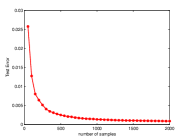
(a) Noise-free data

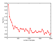
(b) Noise data

Figure 1: Learning capability of [8]’s networks

Fig.1 shows the learning performance of FNN constructed in [8]. The experimental setting in Fig.1 can be found in Section IV. From approximation to learning, the tug of war between bias and variance [11] dictates that besides the approximation capability, a learning system of high quality should take the cost to reach the approximation accuracy into account. Using the constructed FNN for learning is doomed to be overfitting, since the variance is neglected in the literature. A preferable way to reduce the variance is to cut down the number of neurons. Comparing Fig.2(a) with Fig.1(b), we find that selecting part of samples with good geometrical distribution to construct FNN possesses better learning performance than using the whole data.

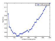
(a) Learning by part of samples

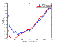
(b) Learning through average

Figure 2: Performance of refined construction of [8]’s networks

It is unreasonable to throw away part of samples and therefore leaves a possibility to improve the learning performance further. Our idea stems from the local average argument in statistics [19], showing that noise-resistent estimators can be derived by averaging samples in a small region. The construction starts with selecting a set of centers (not the samples) with good geometrical distribution and generating the Voronoi partitions [15] based on them. Then, an FNN is constructed according to the well-developed constructive technique in approximation theory [8, 24, 27] by averaging outputs whose corresponding inputs are in the same partition. As the constructed FNN suffers from the well-known saturation phenomenon in the sense that the learning rate cannot be improved once the smoothness of the regression function goes beyond a specific value [19], we present a Landweber-type iterative method to overcome saturation in the last step. As shown in Fig.2(b), the performance of FNN constructed in such a way outperforms the previous FNNs.

I-B Contributions

In this paper, we adopt the ideas from “constructive neural networks” in approximation theory [8, 24, 27], “local average” in statistics [19], “Voronoi partition” in numerical analysis [37, 15] and “Landweber-type iteration for saturation problem” in inverse problems [16, 17] to propose a new scalable learning scheme for FNN. In short, we aim at constructing an FNN, called the constructive feed-forward neural network (CFN) for learning. Our main contributions are three folds.

Firstly, different from the previous optimization-based training schemes [5, 23], our approach shows that parameters of FNN can be constructed directly based on samples, which essentially reduces the computational burden and provides a scalable FNN learning system to tackle massive data. The method is novel in terms of providing a step stone from FNN approximation to FNN learning by using tools in statistics, numerical analysis and inverse problems.

The saturation problem, which was proposed in [8] as an open question, is a classical and long-standing problem of constructive FNN approximation. In fact, all of FNNs constructed in [1, 7, 8, 9, 10, 24, 27] suffer from the saturation problem. We highlight our second contribution to provide an efficient iterative method to overcome the saturation problem without affecting the variance very much.

Our last contribution is the feasibility verification of the proposed CFN. We verify both theoretical optimality and numerical efficiency of it. Theoretically, we prove that if the regression function is smooth, then CFN achieves the optimal learning rate in the sense that the upper and lower bounds are identical and equal to the best learning rates [19]. Experimentally, we run a series of numerical simulations to verify the theoretical assertions on CFN, particularly, the good generalization capability and low computational burden.

I-C Outline

The rest of paper is organized as follows. In the next section, we present the details of CFN. In Section III, we study the theoretical behavior of CFN and compare it with some related work. In Section IV, some simulation results are reported to verify the theoretical assertions. In Section V, we prove the main results. In Section VI, we conclude the paper and present some discussions.

II Construction of CFN

The construction of CFN is based on three factors: a Voronoi partition of the input space, a partition-based distance, and Landweber-type iterations.

II-A Voronoi Partition

Let $\mathcal{X}\subset\mathbf{R}^{d}$ be a compact set and $\Xi_{n}:=\{\xi_{j}\}_{j=1}^{n}$ be a set of points in $\mathcal{X}$. Define the mesh norm $h_{\Xi}$ and separate radius $q_{{}_{\Xi}}$ [37] of $\Xi_{n}$ by

$$h_{\Xi}:=\max_{x\in\mathcal{X}}\min_{j}d(x,\xi_{j}),\quad q_{{}_{\Xi}}:=\frac{1}{2}\min_{1\leq j\neq k\leq n}d(\xi_{j},\xi_{k}),$$

where $d(x,x^{\prime})$ denotes the Euclidean distance between $x$ and $x^{\prime}$. If there exists a constant $\tau\geq 1$ satisfying ${h_{\Xi}}/{q_{{}_{\Xi}}}\leq\tau,$ then $\Xi_{n}$ is said to be quasi-uniform [37] with parameter $\tau$. Throughout the paper, we assume $\Xi_{n}$ is a quasi-uniform set with parameter 2. That is,

$${h_{\Xi}}\leq 2q_{{}_{\Xi}}\leq\frac{1}{n^{d}}\leq 2h_{\Xi}\leq 4q_{{}_{\Xi}}.$$ (2)

Due to the definition of mesh norm, we get

$$\mathcal{X}\subseteq\bigcup_{j=1}^{n}B_{j}(h_{\Xi}),$$

where $B_{j}(r)$ denotes the Euclidean ball with radius $r$ and center ${\xi_{j}}$.

A Voronoi partition $(A_{j})_{j=1}^{n}$ of $\mathcal{X}$ with respect to $\Xi_{n}$ is defined (e.g. [15]) by

$$A_{j}=\left\{x\in\mathcal{X}:j=\min\{\arg\min_{1\leq k\leq n}d(x,\xi_{k})\}\right\}.$$

By definition, $A_{j}$ contains all $x\in\mathcal{X}$ such that the center $\xi_{j}$ is the nearest center to $x$. Moreover, if there exist $j_{1}$ and $j_{2}$ with $j_{1}<j_{2}$, and

$$d(x,\xi_{j_{1}})=d(x,\xi_{j_{2}})<d(x,\xi_{k})$$

for all $k\in\{1,2,\dots,n\}/\{j_{1},j_{2}\}$, then $x\in A_{j_{1}}$, since $j_{1}<j_{2}$. It is obvious that $A_{j}\neq\varnothing$, $A_{j}\subset B_{j}(h_{\Xi})$ for all $j\in\{1,\dots,n\}$, $A_{j_{1}}\cap A_{j_{2}}=\varnothing$ $(j_{1}\neq j_{2})$, and $\mathcal{X}=\bigcup_{j=1}^{n}A_{j}$. Fig.3 (a) presents a specific example of the Voronoi partition in $[0,1]^{2}$. The Voronoi partition is a classical partition technique for scattered data fitting and has been widely used in numerical analysis [37].

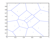
(a) Voronoi partition

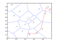
(b) Partition-based distance

Figure 3: Voronoi partition and partition-based distance

II-B Partition-based Distance and the first Order CFN

To introduce the partition-based distance, we rearrange the points in $\Xi_{n}$ in the following way: let $\xi_{1}^{\prime}$ be an arbitrary point in $\Xi_{n}$, and then recursively set $\xi_{j+1}^{\prime}$ satisfying $\|\xi^{\prime}_{j}-\xi^{\prime}_{j+1}\|_{l^{2}}\leq 2h_{\Xi},1\leq j\leq n-1.$ For the sake of brevity, we denote by $\Xi_{n}$ its rearrangement $\{\xi_{j}^{\prime}\}_{j=1}^{n}$. Let $(A_{j})_{j=1}^{n}$ be a Voronoi partition with respect to $\Xi_{n}$. Then, for any $x\in\mathcal{X}$, there exists a unique $k_{0}\leq n$ such that $x\in A_{k_{0}}$. Given any two points $x,x^{\prime}\in X$, we define the partition-based distance between $x\in A_{k_{0}}$ and $x^{\prime}\in A_{j_{0}}$ by

$$\overline{d}(x,x^{\prime})=d(x,x^{\prime}),\quad\mbox{if}\ k_{0}=j_{0},$$

and otherwise

$$\overline{d}(x,x^{\prime})=\sum_{j=\min\{j_{0},k_{0}\}}^{{\max\{j_{0},k_{0}\}}-1}d(\xi_{j},\xi_{j+1})+d(\xi_{k_{0}},x)+d(\xi_{j_{0}},x^{\prime}).$$

In the above definition, $\{\xi_{j}\}_{j=1}^{n}$ are used as freight stations in computing the distance. Fig.3 (b) presents an example for the partition-based distance between $t_{1}$ and $t_{2}$ in $[0,1]^{2}$.

Let $S_{m}=(x_{i},y_{i})_{i=1}^{m}$ be the set of samples and $I_{m}=(x_{i})_{i=1}^{m}$ be the set of inputs. Let $T_{j}=A_{j}\cap{I_{m}}$ be the set of inputs locating in $A_{j}$ ($T_{j}$ may be an empty set). Denote by $T_{j}=\{x_{1}^{j},\dots,x_{|T_{j}|}^{j}\}$ and its corresponding output as $\{y_{1}^{j},\dots,y_{|T_{j}|}^{j}\}$. The first order CFN is given by

$$N^{1}_{n,w}({x}):=\frac{\sum_{i=1}^{|T_{1}|}y_{i}^{1}}{|T_{1}|}+\sum_{j=1}^{n-1}\left(\frac{\sum_{i=1}^{|T_{j+1}|}y_{i}^{j+1}}{|T_{j+1}|}\right.$$

$$-\left.\frac{\sum_{i=1}^{|T_{j}|}y_{i}^{j}}{|T_{j}|}\right)\sigma\left(w\left(\overline{d}(\xi_{1},{x})-\overline{d}(\xi_{1},\xi_{j})\right)\right),$$ (3)

where $w\in\mathbf{R}_{+}$ is a parameter which will be determined in the next section. Here and hereafter, we denote by $\frac{0}{0}=0$.

II-C Iterative Scheme for the $r$th Order CFN

The constructed neural network in (II-B) suffers from the saturation problem. Indeed, it can be found in [8] that the approximation rate of (II-B) cannot exceed $n^{-2/d}$, no matter how smooth the regression function is. Such a saturation phenomenon also exists for the Tikhonov regularization algorithms [17] in inverse problems and Nadaraya-Watson kernel estimate in statistics [19]. It was shown in [17] and [34] that the saturation problem can be avoided by iteratively learning the residual. Borrowing the ideas from [17] and [34], we introduce an iterative scheme to avoid the saturation problem of CFN.

Let $N_{n,w}^{1}(\cdot)$ be defined by (II-B). For $k=1,2,\dots,r-1$, the iterative scheme is processed as follows.

(1) Compute the residuals $e_{i,k}=y_{i}-N^{k}_{n}(x_{i})$, $i=1,2,\dots,m$.

(2) Fit $U^{k}_{n,w}$ to the data $\{{x}_{i},e_{i,k}\},$ $i=1,\dots,m$, i.e.,

$$U^{k}_{n,w}({x}):=\frac{\sum_{i=1}^{|T_{1}|}e_{i,k}^{1}}{|T_{1}|}+\sum_{j=1}^{n-1}\left(\frac{\sum_{i=1}^{|T_{j+1}|}e_{i,k}^{j+1}}{|T_{j+1}|}\right.$$

$$\left.-\frac{\sum_{i=1}^{|T_{j}|}e_{i,k}^{j}}{|T_{j}|}\right)\sigma\left(w\left(\overline{d}(\xi_{1},{x})-\overline{d}(\xi_{1},\xi_{j})\right)\right).$$ (4)

(3) Update $N_{n,w}^{k+1}({x})=N_{n,w}^{k}({x})+U_{n,w}^{k}({x})$.

We obtain the $r$th order CFN $N_{n,w}^{r}$ after repeating the above procedures $r-1$ times.

II-D Summary of CFN

Algorithm 1 CFN

  Step 1 (Initialization): Given data $S_{m}=\{(X_{i},Y_{i}):i=1,\dots,m\}$, the iteration number $r$, the number of neurons $n$, the activation function $\sigma$ and the parameter $w$.

   Step 2 (Sampling): Select $n$ quasi-uniform points $\Xi_{n}:=\{\xi_{j}\}_{j=1}^{n}$ in $\mathcal{X}$.

   Step 3 (Rearranging): Rearrange $n$ quasi-uniform points in $\Xi_{n}$ such that $d(\xi_{j},\xi_{j+1})\leq\frac{2}{n^{1/d}}.$

   Step 4 (Voronoi partition): Present a Voronoi partition with respect to $\Xi_{n}$ and to get a set of subsets $(A_{j})_{j=1}^{n}$ satisfying $A_{j}\cap A_{k}=\varnothing$, and $\cup_{j=1}^{n}A_{j}=\mathcal{X}$.

   Step 5 (Constructing of the first order CFN): Define the first order CFN by (II-B).

   Step 6 (Initializing for iteration): For $k\in\mathbf{N}$, define $e_{i,k}=y_{i}-N^{k}_{n}(x_{i})$ and generate a new set of sample $(x_{i},e_{i,k})_{i=1}^{m}$.

   Step 7 (Iterative updating function): Define the updating function $U_{n,w}^{k}$ by (II-C).

   Step 8 (Updating): Define the $(k+1)$-th order CFN by $N_{n,w}^{k+1}({x})=N_{n,w}^{k}({x})+U_{n,w}^{k}({x})$.

   Step 9 (Iterating): Increase $k$ by one and repeat Step 6-Step 8 if $k<r$, otherwise, the algorithm stops.

The proposed CFN can be formulated in Algorithm 1. In Step 2, we focus on selecting $n$ quasi-uniform points in $\mathcal{X}$. Theoretically, the distribution of $\Xi_{n}$ significantly affects the approximation capability of CFN, as well as the learning performance. Therefore, $\Xi_{n}$ is arranged the more uniform, the better. In practice, we use some well developed low-discrepancy sequences such as the Sobol sequence [6] and the Halton sequence [2] to generate $\Xi_{n}$. As there are some existing matlab codes (such as the “sobolset” comment for the Sobol sequence), we use the Sobol sequence in this paper, which requires $\mathcal{O}(n\log n)$ floating computations to generate $n$ points. In Step 3, to implement the rearrangement, we use the greedy scheme via searching the nearest point one by one. It requires $\mathcal{O}(n^{2})$ floating computations. In Step 4, it requires $\mathcal{O}(n^{2})$ floating computations to generate a Voronoi partition. In Step 5, the partition-based distance requires $\mathcal{O}(n)$ floating computations. Then it can be deduced from (II-B) that there are $\mathcal{O}(mn)$ floating computations in this step. From Step 6 to Step 9, there is an iterative process and it requires $\mathcal{O}(rmn+rn^{2})$ floating computations. Summarily, the total floating computations of Algorithm 1 are of the order $\mathcal{O}(rmn+rn^{2})$.

III Theoretical Behavior

In this section, we analyze the theoretical behavior of CFN in the framework of statistical learning theory [11] and compare it with some related work.

III-A Assumptions and Main Result

Let $S_{m}=(x_{i},y_{i})_{i=1}^{m}\subset\mathcal{Z}:=\mathcal{X}\times\mathcal{Y}$ be a set of samples drawn independently according to an unknown joint distribution $\rho$, which satisfies $\rho(x,y)=\rho_{X}(x)\rho(y|x).$ Here, $\rho_{X}$ is the marginal distribution and $\rho(y|x)$ is the conditional distribution. Without loss of generality, we assume $|y_{i}|\leq M$ almost surely for some positive number $M$. The performance of an estimate, $f$, is measured by the generalization error

$$\mathcal{E}(f):=\int_{\mathcal{Z}}(f(x)-y)^{2}d\rho,$$

which is minimized by the regression function defined by

$$f_{\rho}(x):=\int_{\mathcal{Y}}yd\rho(y|x).$$

Let $L^{2}_{\rho_{{}_{X}}}$ be the Hilbert space of $\rho_{X}$ square integrable functions on $\mathcal{X}$, with norm $\|\cdot\|_{\rho}.$ According to [11], there holds

$$\mathcal{E}(f)-\mathcal{E}(f_{\rho})=\|f-f_{\rho}\|^{2}_{\rho}.$$ (5)

To state the main result, some assumptions on the regression function and the activation function should be imposed. Let $s=u+\beta$ for some $u\in\mathbf{N}$ and $0<\beta\leq 1$. A function $f:\mathcal{X}\rightarrow\mathbf{R}$ is called $s$-smooth if for every $\alpha=(\alpha_{1},\dots,\alpha_{d})$, $\alpha_{l}\in\mathbf{N}$, $\sum_{l=1}^{d}\alpha_{l}=u$ and for all $x,x^{\prime}\in\mathcal{X}$, the partial derivative $\frac{\partial^{u}f}{\partial x_{1}^{\alpha_{1}}\cdots\partial x_{d}^{\alpha_{d}}}$ exists and satisfies

$$\left|\frac{\partial^{u}f}{\partial x_{1}^{\alpha_{1}}\cdots\partial x_{d}^{\alpha_{d}}}(x)-\frac{\partial^{u}f}{\partial x_{1}^{\alpha_{1}}\cdots\partial x_{d}^{\alpha_{d}}}(x^{\prime})\right|\leq C[d(x,x^{\prime})]^{\beta}$$

for some universal positive constant $C$. Let $\mathcal{F}^{s}$ be the set of all $s$-smooth functions.

Assumption 1

$f_{\rho}\in\mathcal{F}^{s}$ for some $s>0$.

Assumption 1 describes the smoothness of $f_{\rho}$, and is a regular assumption in learning theory. It has been adopted in [19, 23, 25, 26, 31] to quantify the learning performance of various neural network-type learning systems. Let $\mathcal{M}(\Theta)$ be the class of all Borel measures $\rho$ on $\mathcal{Z}$ such that $f_{\rho}\in\Theta$. Let $\mathbf{G}_{m}$ be the set of all estimators derived from the sample $S_{m}$. Define

$$e_{m}(\Theta):=\inf_{f_{S}\in\mathbf{G}_{m}}\sup_{\rho\in\mathcal{M}(\Theta)}\mathbf{E}\left\{\|f_{\rho}-f_{S}\|^{2}_{\rho}\right\}.$$

Obviously, $e_{m}(\Theta)$ quantitatively measures the quality of $f_{S}$. It can be found in [19, Th.3.2] or [13, Eq.(3.26)] that

$$e_{m}(\mathcal{F}^{s})\geq C_{0}m^{-\frac{2s}{2s+d}},\ m=1,2,\dots,$$ (6)

where $C_{0}$ is a constant depending only on $C$, $M$, $s$ and $d$. If an $S_{m}$-based estimator $f_{S}$ reaches the bound

$$\sup_{\rho\in\mathcal{M}(\mathcal{F}^{s})}\mathbf{E}\left\{\|f_{\rho}-f_{S}\|^{2}_{\rho}\right\}\leq C_{1}m^{-\frac{2s}{2s+d}},$$

where $C_{1}$ is a constant independent of $m$, then $f_{m}$ is rate-optimal for $\mathcal{F}^{s}$.

Let $\sigma:\mathbf{R}\rightarrow\mathbf{R}$ be a sigmoidal function, i.e.,

$$\lim_{t\rightarrow+\infty}\sigma(t)=1,\quad\lim_{t\rightarrow-\infty}\sigma(t)=0.$$

Then, there exists a $K>0$ such that

$$|\sigma(t)-1|<n^{-(s+d)/d}\quad\mbox{if}\quad t\geq K,$$ (7)

and

$$|\sigma(t)|<n^{-(s+d)/d}\quad\mbox{if}\quad t\leq-K.$$ (8)

For a positive number $a$, we denote by $[a]$, $\lceil a\rceil$, and $\lfloor a\rfloor$ the integer part of $a$, the smallest integer not smaller than $a$ and the largest integer smaller than $a$.

Assumption 2

(i) $\sigma$ is a bounded sigmoidal function.
(ii) For $s>0$, $\sigma$ is at least $\lfloor s\rfloor$ differentiable.

Conditions (i) and (ii) are mild. Indeed, there are numerous examples satisfying (i) and (ii) for arbitrary $s$, such as the logistic function

$$\sigma(t)=\frac{1}{1+e^{-t}},$$

hyperbolic tangent sigmoidal function

$$\sigma(t)=\frac{1}{2}(\tanh(t)+1)$$

with $\tanh(t)=(e^{2t}-1)/(e^{2t}+1)$, arctan sigmoidal function

$$\sigma(t)=\frac{1}{\pi}\arctan(t)+\frac{1}{2},$$

and Gompertz function

$$\sigma(t)=e^{-ae^{-bt}}$$

with $a,b>0$.

The following Theorem 1 is the main result of this paper, which illustrates the rate optimality of CFN.

Theorem 1

Let $s>0$, $r\in\mathbf{N}$ with $r\geq s$ and $N_{n,w}^{r}$ be the estimator defined by Algorithm 1. Under Assumptions 1 and 2, if $n\sim m^{\frac{d}{2s+d}}$ and $w\geq 4Kn^{1/{d}}$ with $K$ satisfying (7) and (8), then there exists a constant $C_{2}$ independent of $m$ or $n$ such that

$$C_{0}m^{-\frac{2s}{2s+d}}\leq\sup_{f_{\rho}\in\mathcal{F}^{s}}\mathbf{E}\left\{\|N_{n,w}^{r}-f_{\rho}\|_{\rho}^{2}\right\}\leq C_{2}m^{-\frac{2s}{2s+d}}.$$ (9)

III-B Remarks and Comparisons

There are three parameters in CFN: the number of centers $n$, the parameter $w$ and the number of iterations $r$. Theorem 1 shows that if some priori information of the regression function is known, i.e., $f_{\rho}\in\mathcal{F}^{s}$, then all these parameters can be determined. In particular, we can set $w\geq 4Kn^{1/d}$, $r=\lceil s\rceil$, and $n=\left[m^{d/(2s+d)}\right].$ $K$ in (7) and (8) depends on $s$, $\sigma$ and $n$. So $K$ can be specified when $\sigma$ and $n$ are given. For example, if the logistic function is utilized, then $w\geq 4\frac{(s+d)n^{1/d}\log n}{d}$ is preferable.

However, in real world applications, it is difficult to check the smoothness of the regression function. We provide some suggestions about the parameter selection. Since Theorem 1 holds for all $w\geq 4Kn^{1/d}$, $w$ can be selected to be sufficiently large. The iterative scheme is imposed only for overcoming the saturation problem and regression functions in real world applications are usually not very smooth. We find that a few iterations (say, $r\leq 5$) are commonly sufficient. Thus, we set $r\in[1,5]$ in real world applications and use the cross-validation [19] to fix it. The key parameter is $n$, which is also crucial for almost all neural network-type learning systems, since $n$ reflects the trade-off between bias and variance. We also use the cross-validation to determine it. Compared with the optimization-based neural network-type learning systems, the total computational complexity of CFN (with cross-validation) is much lower, since the computational complexity of CFN is of order $\mathcal{O}(mn)$ for fixed $r$ and that of optimization-based methods is at least $\mathcal{O}(mn^{2})$ [21].

The saturation problem of FNN approximation was proposed as an open question by Chen [8]. It can be found in [1, 2, 7, 9, 10, 24] that the saturation problem for constructive neural network approximation has not been settled, since all these results were built upon the assumption that the regression function belongs to $\mathcal{F}^{s}$ with $0<s\leq 1$. However, for optimization-based FNN, the saturation problem did not exist as shown in the prominent work [29, 30]. In the present paper, we succeed in settling the saturation problem by using the proposed iterative scheme. Theorem 1 states that if $f_{\rho}\in\mathcal{F}^{s}$, then CFN is rate-optimal for all $s>0$, since its learning rate can reach the base line (6).

Finally, we compare Theorem 1 with two related theoretical results about learning performance of optimization-based FNN learning [31] and extreme learning machine (ELM) [26]. Denote

$$\mathcal{N}^{M}_{n}:=\left\{f=\sum_{k=1}^{n}c_{k}\phi(a_{k}\cdot x+b_{k}):\|f\|_{\infty}\leq M\right\},$$

where $a_{k}\in\mathbf{R}^{d}$, $b_{k},c_{k}\in\mathbf{R}$. Define

$$f_{1,S}=\arg\min_{f\in\mathcal{N}^{M}_{n}}\frac{1}{m}\sum_{i=1}^{m}(f(x_{i})-y_{i})^{2}.$$ (10)

Maiorov [31] proved that for some activation function $\phi$, if $f_{\rho}\in\mathcal{F}^{s}$ and $n\sim m^{d/(s+d)}$, then there holds

$$C_{0}m^{-\frac{2s}{2s+d}}\leq\sup_{f_{\rho}\in\mathcal{F}^{s}}\mathbf{E}\left\{\|f_{1,S}-f_{\rho}\|_{\rho}^{2}\right\}\leq C_{3}m^{-\frac{2s}{2s+d}}\log m,$$ (11)

where $C_{3}$ is a constant independent of $m$ or $n$. It should be noted from (10) that $f_{1,S}$ is obtained by solving a nonlinear least squares problem, which generally requires higher computational complexity than CFN. Furthermore, comparing (9) with (11), we find that CFN is rate-optimal while (10) is near rate-optimal (up to a logarithmic factor).

Denote

$$\mathcal{N}^{R}_{n}:=\left\{f=\sum_{k=1}^{n}c_{k}\phi(a^{*}_{k}\cdot x+b^{*}_{k}):c_{k}\in\mathbf{R}\right\},$$

where $a^{*}_{k}\in\mathbf{R}^{d}$, $b^{*}_{k}\in\mathbf{R}$ are randomly selected according to a distribution $\mu$. The ELM estimator is defined by

$$f_{2,S}=\arg\min_{f\in\mathcal{N}^{R}_{n}}\frac{1}{m}\sum_{i=1}^{m}(f(x_{i})-y_{i})^{2}.$$ (12)

It is easy to see that the optimization problem (12) is a linear problem and can be solved by using the pseudo-inverse technique [21]. The theoretical performance of ELM was justified in [26], which asserts that for some activation function, if $f_{\rho}\in\mathcal{F}^{s}$ and $n\sim m^{d/(s+d)}$, then there holds

$$\mathbf{E}_{\mu}\mathbf{E}\left\{\|f_{2,S}-f_{\rho}\|_{\rho}^{2}\right\}\leq C_{4}m^{-\frac{2s}{2s+d}}\log m,$$ (13)

where $C_{4}$ is a constant independent of $m$ or $n$. It follows from (6) and (13) that (12) is near rate-optimal in the sense of expectation, since there is an additional $\mathbf{E}_{\mu}$ in (13) due to the randomness of $f_{2,S}$. Compared with (13), our result in (9) shows that CFN can remove the logarithmic factor and avoid the randomness of ELM.

IV Simulations

In this section, we verify our theoretical assertions via a series of numerical simulations. When $d=1$, the rearranging step (Step 3 in Alg.1) is trivial. Thus, we divide the simulations into two cases: $d=1$ and $d>1$. All numerical studies are implemented by using MATLAB R2014a on a Windows personal computer with Core(TM) i7-3770 3.40GHz CPUs and RAM 4.00GB. Throughout the simulations, the logistic activation function is used and the statistics are averaged based on 20 independent trails.

IV-A Simulations for $d=1$

In the simulations, we generate training data from the following model:

$$Y=f(X)+\varepsilon,$$ (14)

where $\varepsilon$ is the Gaussian noise with variance $0.1$ and independent of $X$. The centers are $n$ equally spaced points in $[-1,1]$. The test data are sampled from $Y=f(X)$. Let

$$f_{1}(x)=1+\frac{80}{3}x^{2}-40x^{3}+15x^{4}+\frac{8}{3}x^{5}+20x^{2}\log(|x|),$$

and

$$f_{2}(x)=(1-x)_{+}^{5}(8x^{2}+5x+1),$$

where $a_{+}=a$ when $a\geq 0$ and $a_{+}=0$ when $a<0$. It is easy to check that $f_{1}\in\mathcal{F}^{1}$ but $f_{1}\notin\mathcal{F}^{2}$ and $f_{2}\in\mathcal{F}^{4}$ but $f_{2}\notin\mathcal{F}^{5}$.

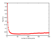
(a) Role of $n$ for $f_{1}$

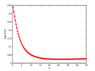
(b) Role of $w$ for $f_{1}$

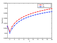
(c) Role of $r$ for $f_{1}$ and $f_{2}$

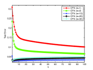
(d) Small $w$ and large $r$ for $f_{1}$

Figure 4: Roles of parameters

In the first simulation, we numerically study the roles of three parameters $n$, $w$, and $r$. Since we are interested in the role of a specified parameter, the other two parameters are selected to be optimal according to the test data directly. In this simulation, the number of training and test samples are 1024 and 1000. The results of the simulation are shown in Fig.4. Fig.4 (a) describes the relation between the test error and the number of centers. From Fig.4 (a), it follows that there exists an optimal $n$ ranged in $[10,20]$ minimizing the test error, which coincides with the theoretical assertions $n\sim m^{d/(2s+d)}=1024^{1/3}$. Fig.4 (b) demonstrates the relation between the test error and $w$. It can be found in Fig.4 (b) that after a crucial value of $w$, the test error does not vary with respect to $w$, which coincides with the assertion in Theorem 1. Fig.4 (c) presents the relation between the test error and the number of iterations. It is shown in Fig.4 (c) that such a scheme is feasible and can improve the learning performance. Furthermore, there is an optimal $r$ in the range of $[1,5]$ minimizing the test error (the average value of $r$ is $2.2$ via average for 20 trails). This also verifies our assertions in Sec.III. Fig.4 (d) presents another application of the iterative scheme in CFN. It is shown in Fig.4 (d) that once the parameter $w$ is selected to be small, then we can use large $r$ to reduce the test error.

TABLE I: Comparisons of learning performance for $d=1$.

	TrainRMSE	TestRMSE	TrainingTime	TestTime
$f_{1}$
CFN	0.3305(0.0070)	0.0182(0.0035)	0.51[0.01]	0.91
RLS	0.3303(0.0070)	0.0203(0.0064)	9.95[0.19]	8.22
ELM	0.3302(0.0070)	0.0223(0.0072)	0.42[0.01]	0.31
$f_{2}$
CFN	0.3304(0.0070)	0.0199(0.0037)	0.48[0.01]	0.88
RLS	0.3303(0.0070)	0.0204(0.0067)	10.6[0.21]	9.14
ELM	0.3302(0.0070)	0.0225(0.0072)	0.42[0.01]	0.33

In the second simulation, we compare CFN with two widely used learning schemes. One is the regularized least square (RLS) with Gaussian kernel [14], which is recognized as the benchmark for regression. The other is the extreme learning machine (ELM) [21], which is one of the most popular neural network-type learning systems. The corresponding parameters including the width of the Gaussian kernel and the regularization parameters in RLS, the number of hidden neurons in ELM, and the number of centers, the number of iterations in CFN are selected via five-fold cross validation. We record the mean test RMSE (rooted square mean error) and the mean training RMSE as TestRMSE and TrainRMSE, respectively. We also record their standard deviations in the parentheses. Furthermore, we record the average total training time as TrainTime. We also record the time of training for fixed parameters in the bracket. Since the training time of ELM is different for different number of neurons, we record in the bracket the training time for ELM with optimal parameter. We finally record the mean test time as TestTime. The results are reported in Table I. It is shown in Table I that the learning performance of CFN is at least not worse than RLS and ELM. In fact, the test error of CFN is comparable with RLS but better than ELM and the training price (training time and memory requirement) of CFN is comparable with ELM but lower than RLS. This verifies the feasibility of CFN and coincides with our theoretical assertions.

IV-B Simulations for $d>1$

When $d>1$, the strategies of selecting centers and rearrangement operator are required. In this part, we draw the Sobol sequence to build up the set of centers and then use a greedy strategy to rearrange them. Specifically, we start with an arbitrary point in the Sobol sequence, then select the next point to be the nearest point of the current point, and then repeat this procedure until all the points are rearranged. We show in the following Fig.5 that such a greedy scheme essentially cuts down the maximum distance between arbitrary two adjacent points (max dist). For comparison, we also exhibit the change of the minimum distance (min dist).

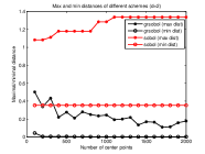
(a) $d=2$

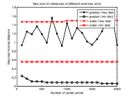
(b) $d=5$

Figure 5: Distribution of centers

We demonstrate the feasibility of CFN by comparing it with RLS and ELM for various regression functions. Let

$$f_{3}(x)=(1-\|x\|_{2})_{+}^{6}(35/3\|x\|_{2}^{2}+6\|x\|_{2}+1),$$

$$f_{4}(x)= (1-\|x\|_{2})_{+}^{7}(35\|x\|_{2}^{6}+245\|x\|_{2}^{5}+720\|x\|_{2}^{4}$$

$$+1120\|x\|_{2}^{3}+928\|x\|_{2}^{2}+336\|x\|_{2}+48),$$

and

$$f_{5}(x)= 1+\frac{80}{3}\|x\|_{2}^{5}-40\|x\|_{2}^{3}+15\|x\|_{2}^{4}+\frac{8}{3}\|x\|_{2}^{5}$$

$$+20\|x\|_{2}^{2}log(\|x\|_{2}),$$

where $\|x\|_{2}$ denotes the Euclidean norm of the vector $x$. It is easy to check that for $d=2,3,5$, $f_{5}\in\mathcal{F}^{1}$ but $f_{5}\notin\mathcal{F}^{2}$ and for $d=2,3$, $f_{3}\in\mathcal{F}^{4}$ but $f_{3}\notin\mathcal{F}^{5}$ and for $d=5$, $f_{4}\in\mathcal{F}^{4}$ but $f_{4}\notin\mathcal{F}^{5}$. The simulation results are reported in Table II. It can be found in Table II that, similar as the one-dimensional simulations, the learning performance of CFN is a bit better than RLS (in time) and ELM (in test error). This also verifies our theoretical assertions.

TABLE II: Comparisons of learning performance for $d>1$.

	TrainRMSE	TestRMSE	TrainingTime	TestTime
$f_{3}$, $d=2$
CFN	0.3303(0.010)	0.0341 (0.0094)	4.67 [0.067]	1.05
RLS	0.3259(0.0102)	0.0412(0.0047)	10.6[0.217]	9.43
ELM	0.3291(0.010)	0.0391 (0.0055)	0.42 [0.003]	0.34
$f_{3}$, $d=3$
CFN	0.3312 (0.008)	0.0495 (0.0057)	4.77[0.09]	1.05
RLS	0.3204(0.007)	0.0593(0.0065)	11.0 [0.27]	9.65
ELM	0.3253(0.007)	0.0542 (0.0066)	0.61 [0.01]	0.31
$f_{4}$, $d=5$
CFN	0.3302(0.009)	0.0278(0.004)	4.96 [0.09]	1.12
RLS	0.3294(0.009)	0.0272 (0.006)	10.8 [0.20]	9.79
ELM	0.3303(0.009)	0.0311(0.004)	0.52[0.01]	0.35
$f_{5}$, $d=2$
CFN	0.3318(0.010)	0.0286(0.007)	4.73 [0.08]	0.81
RLS	0.3282(0.011)	0.0404 (0.006)	10.8 [0.22]	9.70
ELM	0.3302 (0.011)	0.0359 (0.007)	0.49 [0.01]	0.45
$f_{5}$, $d=3$
CFN	0.3361(0.009)	0.0465 (0.009)	4.86[0.08]	0.82
RLS	0.3260(0.007)	0.0573 (0.006)	10.6 [0.21]	9.63
ELM	0.3315(0.008)	0.0494 (0.004)	0.56 [0.01]	0.38
$f_{5}$, $d=5$
CFN	0.3310(0.007)	0.0299 (0.006)	4.91 [0.08]	0.80
RLS	0.3270(0.007)	0.0400 (0.003)	10.7 [0.20]	9.77
ELM	0.3329( 0.007)	0.0438(0.004)	0.51 [0.01]	0.47

IV-C Challenge for massive data

Since our main motivation for introducing CFN is to tackle massive data, we pursue the advantage of CFN for massive data sets. For this purpose, we set the number of training data to be $50000,100000,150000$ and the number of test data to be $100000,200000,300000$. As the memory requirements and training time of RLS are huge, we only compare CFN with ELM in this simulation. The simulation results are reported in Table III. It is shown that when applied to the massive data, the performance of CFN is at least not worse than that of ELM. In particular, CFN possesses a slight smaller test errors and dominates in the training time. The reason is that for massive data, a large number of neurons in ELM and CFN are required. When $r\leq 5$ and $n\leq m$, the computational complexities of CFN and ELM are $\mathcal{O}(mn)$ and $\mathcal{O}(mn^{2})$, respectively. Large $n$ inevitably leads to much more training time for ELM. Thus, besides the perfect theoretical behaviors, CFN is also better than ELM when tackling massive data.

TABLE III: Comparisons of learning performance for massive data.

	TrainRMSE	TestRMSE	TrainTime	TestTime
$f_{1}$, $d=1,m=5\times 10^{4}$
CFN	0.3298(0.001)	0.0033(5.0e-004)	13.6[0.34]	21.8
ELM	0.3298(0.001)	0.0035(7.0e-004)	78.9[0.16]	19.2
$f_{1}$, $d=1,m=10^{5}$
CFN	0.3299(0.001)	0.0029(7.3e-004)	28.3[0.71]	45.3
ELM	0.3299(0.001)	0.0027(5.3e-004)	167[ 3.90]	38.3
$f_{1}$, $d=1,m=1.5\times 10^{5}$
CFN	0.3303(0.001)	0.0021(4.8e-004)	42.5[1.27]	67.8
ELM	0.3303(0.001)	0.0022(6.6e-004)	252[7.65]	55.8
$f_{5}$, $d=5,m=5\times 10^{4}$
CFN	0.3309(0.001)	0.0161(0.005)	95.8[4.51]	44.6
ELM	0.3304(0.001)	0.019(0.001)	134[2.70]	36.5
$f_{5}$, $d=5,m=10^{5}$
CFN	0.3302(0.001)	0.0131(5.0e-04 )	191[8.93]	89.1
ELM	0.3299(0.001)	0.0159(7.0e-04 )	260[7.05]	71.6
$f_{5}$, $d=5,m=1.5\times 10^{5}$
CFN	0.3307(0.001)	0.0122(3.9e-04)	291[13.2]	134
ELM	0.3305(0.001)	0.0138(6.6e-04)	399[9.81]	108

V Proof of Theorem 1

The lower bound of (9) can be derived directly by (6). Therefore, it suffices to prove the upper bound of (9). For $1\leq k\leq r$, define

$$\widetilde{N_{n,w}^{k}}(x):=\mathbf{E}\left[N_{n,w}^{k}(x)|X_{1},\dots,X_{m}|\right].$$

Then,

$$\mathbf{E}\left[\|N_{n,w}^{r}-f_{\rho}\|_{\rho}^{2}\right]$$

$$= \mathbf{E}\left[\|N_{n,w}^{r}-\widetilde{N_{n,w}^{r}}\|_{\rho}^{2}\right]+\mathbf{E}\left[\|\widetilde{N_{n,w}^{r}}-f_{\rho}\|_{\rho}^{2}\right],$$

since $\mathbf{E}\langle N_{n,w}^{r}-\widetilde{N_{n,w}^{r}},\widetilde{N_{n,w}^{r}}-f_{\rho}\rangle_{\rho}=0.$ We call the first term in the righthand of (V) as the sample error (or estimate error) and the second term as the approximation error.

V-A Bounding Sample Error

We divide the bounding of sample error into two cases: $r=1$ and $r>1$. We first consider the case $r=1$. Since $f_{\rho}(x)=\mathbf{E}[Y|X=x]$, we have

$$\widetilde{N_{n,w}^{1}}(x)=\frac{\sum_{i=1}^{|T_{1}|}f_{\rho}(X_{i}^{1})}{|T_{1}|}+\sum_{j=1}^{n-1}\left(\frac{\sum_{i=1}^{|T_{j+1}|}f_{\rho}(X_{i}^{j+1})}{|T_{j+1}|}\right.$$

$$-\left.\frac{\sum_{i=1}^{|T_{j}|}f_{\rho}(X_{i}^{j})}{|T_{j}|}\right)\sigma\left(w\left(\overline{d}(\xi_{1},{x})-\overline{d}(\xi_{1},\xi_{j})\right)\right).$$ (16)

Denote

$$g_{j}:=\frac{\sum_{i=1}^{|T_{j}|}Y_{i}^{j}}{|T_{j}|}=\sum_{i=1}^{m}Y_{i}\frac{I_{\{X_{i}\in A_{j}\}}}{\sum_{l=1}^{m}I_{\{X_{l}\in A_{l}\}}},$$

and

$$g_{j}^{*}:=\frac{\sum_{i=1}^{|T_{j}|}f_{\rho}(X_{i}^{j})}{|T_{j}|}=\sum_{i=1}^{m}f_{\rho}(X_{i})\frac{I_{\{X_{i}\in A_{j}\}}}{\sum_{l=1}^{m}I_{\{X_{l}\in A_{l}\}}},$$

where $I_{A}$ denotes the indicator function of set $A$. Define further

$$c_{1}(x):=1-\sigma(w\overline{d}(\xi_{1},x)),$$

$$c_{n}(x):=\sigma\left(w(\overline{d}(\xi_{1},x)-\overline{d}(\xi_{1},\xi_{n-1})\right),$$

and

$$c_{j}(x):=\sigma\left(w(\overline{d}(\xi_{1},x)-\overline{d}(\xi_{1},\xi_{j-1}))\right)$$

$$-\sigma\left(w(\overline{d}(\xi_{1},x)-\overline{d}(\xi_{1},\xi_{j}))\right),\ 2\leq j\leq n-1,$$

We have

$$N_{n,w}^{1}(x)=\sum_{j=1}^{n}g_{j}c_{j}(x),$$ (17)

and

$$\widetilde{N_{n,w}^{1}}(x)=\sum_{j=1}^{n}g_{j}^{*}c_{j}(x).$$ (18)

Since $A_{j_{1}}\cap A_{j_{2}}=\varnothing$ ($j_{1}\neq j_{2}$) and $\mathcal{X}=\bigcup_{j=1}^{n}A_{j}$, for arbitrary $x$, there is a unique $k_{0}$ such that $x\in A_{k_{0}}$. Without loss of generality, we assume $k_{0}\geq 2$. Then it follows from (2) and the definition of $\overline{d}(\xi_{1},{x})$ that

$$\overline{d}(\xi_{1},{x})-\overline{d}({\xi_{1},\xi_{k}})\geq\frac{1}{4}n^{-1/d},\ 1\leq k\leq k_{0}-1,$$

$$|\overline{d}(\xi_{1},{x})-\overline{d}(\xi_{1},\xi_{k_{0}})|\leq 2n^{-1/d},$$

and

$$\overline{d}(\xi_{1},{x})-\overline{d}({\xi_{1},\xi_{k}})\leq-\frac{1}{4}n^{-1/d},\ k\geq k_{0}+1.$$

Due to (7), (8) and $w\geq 4Kn^{1/d}$, we have when $k\leq k_{0}-1$

$$\left|\sigma\left(w\left(\overline{d}(\xi_{1},{x})-\overline{d}(\xi_{1},\xi_{k})\right)\right)-1\right|<n^{-(s+d)/d},$$ (19)

and when $k\geq k_{0}+1$,

$$\left|\sigma\left(w\left(\overline{d}(\xi_{1},{x})-\overline{d}(\xi_{1},\xi_{k})\right)\right)\right|<n^{-(s+d)/d}.$$ (20)

Then for arbitrary $j\leq k_{0}-1$ and $j\geq k_{0}+2$, (19), (20) and the definition of $c_{j}(x)$ yield

$$|c_{j}(x)|\leq 2n^{-(s+d)/d}.$$

Since $|Y_{j}|\leq M$ almost surely, we have $|g_{j}|\leq M$ and $|g^{*}_{j}|\leq M$ almost surely $j=1,\dots,n$. As

$$\mathbf{E}\left[g_{j}|X_{1},\dots,X_{m}\right]=g_{j}^{*},$$

we get

$$\mathbf{E}\left[(N_{n,w}^{1}(x)-\widetilde{N_{n,w}^{1}}(x))^{2}|X_{1},\dots,X_{m}\right]$$

$$\leq 2M^{2}n^{-2s/d}$$

$$+ \mathbf{E}\left[((g_{k_{0}}-g_{k_{0}}^{*})c_{k_{0}}(x))^{2}|X_{1},\dots,X_{m}\right]$$

$$+ \mathbf{E}\left[((g_{k_{0}+1}-g_{k_{0}+1}^{*})c_{k_{0}+1}(x))^{2}|X_{1},\dots,X_{m}\right].$$

We hence only need to bound

$$\mathbf{E}\left[((g_{k_{0}}-g_{k_{0}}^{*})c_{k_{0}}(x))^{2}|X_{1},\dots,X_{m}\right],$$

since

$$\mathbf{E}\left[((g_{k_{0}+1}-g_{k_{0}+1}^{*})c_{k_{0}+1}(x))^{2}|X_{1},\dots,X_{m}\right]$$

can be bounded by using the same method. As $\sigma$ is bounded, we have

$$\mathbf{E}\left[((g_{k_{0}}-g_{k_{0}}^{*})c_{k_{0}}(x))^{2}|X_{1},\dots,X_{m}\right]$$

$$\leq 4\|\sigma\|^{2}_{\infty}\mathbf{E}\left[(g_{k_{0}}-g_{k_{0}}^{*})^{2}|X_{1},\dots,X_{m}\right].$$

Due to the definition of $g_{k_{0}}$ and $g^{*}_{k_{0}}$, we get

$$\mathbf{E}\left[((g_{k_{0}}-g_{k_{0}}^{*}))^{2}|X_{1},\dots,X_{m}\right]$$

$$= \frac{\sum_{i=1}^{m}(Y_{i}-f_{\rho}(X_{i}))^{2}I_{\{X_{i}\in A_{k_{0}}\}}}{(m\mu_{m}(A_{k_{0}}))^{2}}$$

$$\leq \frac{4M^{2}}{m\mu_{m}(A_{k_{0}})}I_{\{m\mu_{m}(A_{k_{0}})>0\}},$$

where $\mu_{m}(A_{k_{0}})$ denotes the empirical measure of $A_{k_{0}}$. Then it can be found in [19, P65-P66] that

$$\mathbf{E}\left[\frac{I_{\{m\mu_{m}(A_{k_{0}})>0\}}}{m\mu_{m}(A_{k_{0}})}\right]\leq\frac{4n}{m}.$$

This implies

$$\mathbf{E}\left[\|N_{n,w}^{1}-\widetilde{N_{n,w}^{1}}\|_{\rho}^{2}\right]$$

$$= \mathbf{E}\left[\mathbf{E}\left[(N_{n,w}^{1}(X)-\widetilde{N_{n,w}^{1}}(X))^{2}|X,X_{1},\dots,X_{m}\right]\right]$$

$$\leq 2M^{2}n^{-2s/d}+32\|\sigma\|_{\infty}^{2}M^{2}{n}/{m}.$$

Since $n\sim m^{d/(2s+d)}$, we obtain

$$\mathbf{E}\left[\|N_{n,w}^{1}-\widetilde{N_{n,w}^{1}}\|_{\rho}^{2}\right]\leq C^{\prime}m^{-2s/(2s+d)},$$ (21)

where $C^{\prime}$ is a constant depending only on $M$.

We then bound the sample error for $r>1$. It follows from the definition of $N_{n,w}^{k+1}(x)$ that

$$N_{n,w}^{k+1}(x)=N_{n,w}^{k}(x)+N_{n,w}^{1}(x)$$

$$- \frac{\sum_{i=1}^{|T_{1}|}(N^{k}_{n,w}(X_{i}^{1}))}{|T_{1}|}-\sum_{j=1}^{n-1}\left(\frac{\sum_{i=1}^{|T_{j+1}|}(N^{k}_{n,w}(X_{i}^{j+1}))}{|T_{j+1}|}\right.$$

$$- \left.\frac{\sum_{i=1}^{|T_{j}|}(N^{k}_{n,w}(X_{i}^{j}))}{|T_{j}|}\right)\sigma\left(w\left(\overline{d}(\xi_{1},{x})-\overline{d}(\xi_{1},\xi_{j})\right)\right),$$

where we denotes the element of $T_{j}$ as $X_{1}^{j},X_{2}^{j},\dots,X_{|T_{j}|}^{j}$. Since

$$\frac{\sum_{i=1}^{|T_{1}|}(N^{k}_{n}(X_{i}^{1}))}{|T_{1}|}+\sum_{j=1}^{n-1}\left(\frac{\sum_{i=1}^{|T_{j+1}|}(N^{k}_{n}(X_{i}^{j+1}))}{|T_{j+1}|}\right.$$

$$- \left.\frac{\sum_{i=1}^{|T_{j}|}(N^{k}_{n}(X_{i}^{j}))}{|T_{j}|}\right)\sigma\left(w\left(\overline{d}(\xi_{1},{x})-\overline{d}(\xi_{1},\xi_{j})\right)\right).$$

is independent of $Y_{1},\dots,Y_{m}$, and

$$\widetilde{N_{n,w}^{k}}(x)=\mathbf{E}\left[N_{n,w}^{k}(x)|X_{1},\dots,X_{m}|\right],$$

we have

$$\mathbf{E}\left[(N_{n,w}^{k+1}(x)-\widetilde{N_{n,w}^{k+1}}(x))^{2}|X_{1},\dots,X_{m}\right]$$

$$\leq 2\mathbf{E}\left[(N_{n,w}^{1}(x)-\widetilde{N_{n,w}^{1}}(x))^{2}|X_{1},\dots,X_{m}\right]$$

$$+ 2\mathbf{E}\left[(N_{n,w}^{k}(x)-\widetilde{N_{n,w}^{k}}(x))^{2}|X_{1},\dots,X_{m}\right].$$

Therefore, we obtain

$$\mathbf{E}\left[\|N_{n,w}^{r}-\widetilde{N_{n,w}^{r}}\|_{\rho}^{2}\right]\leq 2r\mathbf{E}\left[\|N_{n,w}^{1}-\widetilde{N_{n,w}^{1}}\|_{\rho}^{2}\right].$$

Then it follows from (21) that

$$\mathbf{E}\left[\|N_{n,w}^{r}-\widetilde{N_{n,w}^{r}}\|_{\rho}^{2}\right]\leq 2rC^{\prime}m^{-2s/(2s+d)}.$$ (22)

V-B Bounding Approximation Error

It is obvious that

$$(\widetilde{N_{n,w}^{r}}(x)-f_{\rho}(x))^{2}$$

$$= (\widetilde{N_{n,w}^{r}}(x)-f_{\rho}(x))^{2}I_{\{\mu_{m}(A_{k_{0}})>0\}}$$

$$+ (\widetilde{N_{n,w}^{r}}(x)-f_{\rho}(x))^{2}I_{\{\mu_{m}(A_{k_{0}})=0\}}.$$

Due to the definition, we obtain

$$\|\widetilde{N_{n,w}^{r}}\|_{\infty}\leq(2\|\sigma\|_{\infty}+1)rM$$

almost surely. Then it follows from [19, P66-P67] that

$$\mathbf{E}\left[(\widetilde{N_{n,w}^{r}}(X)-f_{\rho}(X))^{2}I_{\{\mu_{m}(A_{k_{0}})=0\}}\right]$$

$$\leq 3(2\|\sigma\|_{\infty}+1)^{2}r^{2}M^{2}\frac{n}{m}.$$

Furthermore,

$$(\widetilde{N_{n,w}^{r}}(x)-f_{\rho}(x))^{2}I_{\{\mu_{m}(A_{k_{0}})>0\}}$$

$$= (\widetilde{N_{n,w}^{r}}(x)-f_{\rho}(x))^{2}I_{\{\mu_{m}(A_{k_{0}})>0,\mu_{m}(A_{k_{0}+1})>0\}}$$

$$+ (\widetilde{N_{n,w}^{r}}(x)-f_{\rho}(x))^{2}I_{\{\mu_{m}(A_{k_{0}})>0,\mu_{m}(A_{k_{0}+1})=0\}}.$$

Similar method in [19, P66-P67] yields

$$\mathbf{E}\left[(\widetilde{N_{n,w}^{r}}(X)-f_{\rho}(X))^{2}I_{\{\mu_{m}(A_{k_{0}})>0,\mu_{m}(A_{k_{0}+1})=0\}}\right]$$

$$\leq 3(2\|\sigma\|_{\infty}+1)^{2}r^{2}M^{2}\frac{n}{m}.$$

Hence, we have

$$\mathbf{E}\left[(\widetilde{N_{n,w}^{r}}(X)-f_{\rho}(X))^{2}\right]$$

$$\leq 6(2\|\sigma\|_{\infty}+1)^{2}r^{2}M^{2}\frac{n}{m}$$

$$+ \mathbf{E}\left[(\widetilde{N_{n,w}^{r}}(X)-f_{\rho}(X))^{2}I_{\{\mu_{m}(A_{k_{0}})>0,\mu_{m}(A_{k_{0}+1})>0\}}\right].$$

To bound

$$\mathbf{E}\left[(\widetilde{N_{n,w}^{r}}(X)-f_{\rho}(X))^{2}I_{\{\mu_{m}(A_{k_{0}})>0,\mu_{m}(A_{k_{0}+1})>0\}}\right],$$

we need to introduce a series of auxiliary functions. Let $X_{j}^{*}$ be arbitrary sample in $A_{j}$ and $Y_{j}^{*}$ be its corresponding output. If there is no point in $A_{j}$, then we denote by $Y_{j}^{*}=0$, and $g(X_{j}^{*})=0$ for arbitrary function $g$. Define

$$L^{1}_{n,w}({x})=f_{\rho}(X_{1}^{*})+\sum_{j=1}^{n-1}\left(f_{\rho}(X_{j+1}^{*})-f_{\rho}(X_{j}^{*})\right)$$

$$\times \sigma\left(w\left(\overline{d}(\xi_{1},{x})-\overline{d}(\xi_{1},\xi_{j})\right)\right),$$

and

$$L^{k+1}_{n,w}({x})=L^{k}_{n,w}({x})+V^{k}_{n,w}({x})$$

with

$$V^{k}_{n,w}({x})=f_{\rho}(X^{*}_{1})-L^{k}_{n}(X_{1}^{*})$$

$$+ \sum_{j=1}^{n-1}\left((f_{\rho}(X_{j+1}^{*})-L^{k}_{n}(X_{j+1}^{*}))\right.$$

$$- \left.(f_{\rho}(X^{*}_{j})-L^{k}_{n}(X^{*}_{j}))\right)\sigma\left(w\left(\overline{d}(\xi_{1},{x})-\overline{d}(\xi_{1},\xi_{j})\right)\right).$$

Then for arbitrary $x\in\mathcal{X}$ and $1\leq k\leq r$, there holds

$$\left|\widetilde{N_{n,w}^{k}}(x)-f_{\rho}(x)\right|\leq\max_{X_{1}^{*},\dots,X_{n}^{*}}\left|L^{k}_{n,w}(x)-f_{\rho}(x)\right|,$$ (24)

where the maximum runs over all the possible choices of $X_{j}^{*}\in A_{j}$, $j=1,2,\dots,n$.

Due to the definition of $c_{j}(x)$, we get

$$L^{1}_{n,w}(x)=\sum_{j=1}^{n}f_{\rho}(X_{j}^{*})c_{j}(x),\quad\mbox{ and}\ \sum_{j=1}^{n}c_{j}(x)=1.$$

We then prove that for arbitrary $k\geq 1$, there exists a set of functions $\{c_{j}^{k}(x)\}_{j=1}^{n}$ such that

$$L^{k}_{n,w}(x)=\sum_{j=1}^{n}f_{\rho}(X_{j}^{*})c^{k}_{j}(x),\ \mbox{and}\ \sum_{j=1}^{n}c_{j}^{k}(x)=1.$$ (25)

We prove (25) by induction. (25) holds for $k=1$ with $c_{j}^{1}(x)=c_{j}(x)$. Assume (25) holds for $l\geq 1$, that is,

$$L^{l}_{n,w}(x)=\sum_{j=1}^{n}f_{\rho}(X_{j}^{*})c^{l}_{j}(x),\ \mbox{and}\ \sum_{j=1}^{n}c_{j}^{l}(x)=1.$$

Obviously,

$$V^{l}_{n,w}({x})=\sum_{j=1}^{n}(f_{\rho}(X_{j}^{*})-L^{l}_{n,w}(X_{j}^{*}))c_{j}^{1}(x).$$

Therefore,

$$L^{l+1}_{n,w}(x)=L^{l}_{n,w}(x)+V^{l}_{n,w}({x})=\sum_{j=1}^{n}f_{\rho}(X_{j}^{*})c^{l}_{j}(x)$$

$$+ \sum_{j=1}^{n}\left(f_{\rho}(X_{j}^{*})-\sum_{i=1}^{n}f_{\rho}(X_{i}^{*})c^{l}_{i}(X_{j}^{*})\right)c_{j}^{1}(x)$$

$$= \sum_{j=1}^{n}f_{\rho}(X_{j}^{*})\left(c^{l}_{j}(x)+c_{j}^{1}(x)-\sum_{i=1}^{n}c_{j}^{l}(X_{i}^{*})c_{i}^{1}(x)\right).$$

Define

$$c^{l+1}_{j}(x):=c^{l}_{j}(x)+c_{j}^{1}(x)-\sum_{i=1}^{n}c_{j}^{l}(X_{i}^{*})c_{i}^{1}(x).$$ (26)

Then it follows from $\sum_{j=1}^{n}c_{j}^{1}(x)=1$ and $\sum_{j=1}^{n}c_{j}^{l}(x)=1$ that

$$\sum_{j=1}^{n}c_{j}^{l+1}(x)=2-\sum_{i=1}^{n}\sum_{j=1}^{n}c_{j}^{l}(X_{i}^{*})c_{i}^{1}(x)=1.$$

This proves (25). (25) together with (26) implies

$$L^{k+1}_{n,w}(x)-f_{\rho}(x)=\sum_{j=1}^{n}c^{k+1}_{j}(x)(f_{\rho}(X_{j}^{*})-f_{\rho}(x))$$

$$= \sum_{j=1}^{n}c^{k}_{j}(x)(f_{\rho}(X_{j}^{*})-f_{\rho}(x))$$

$$- \sum_{i=1}^{n}c_{i}^{1}(x)\left[\sum_{j=1}^{n}c^{k}_{j}(X_{i}^{*})(f_{\rho}(X_{j}^{*})-f_{\rho}(X_{i}^{*}))\right]$$

$$= L^{k}_{n,w}(x)-f_{\rho}(x)-\sum_{j=1}^{n}c^{1}_{j}(x)(L^{k}_{n,w}(X_{j}^{*})-f_{\rho}(X_{j}^{*})).$$

If we denote by $\lambda^{k}(x):=L^{k}_{n,w}(x)-f_{\rho}(x)$ with $\lambda^{0}(x):=f_{\rho}(x)$, then

$$\lambda^{k+1}(x)=\lambda^{k}(x)-\sum_{j=1}^{n}c^{1}_{j}(x)\lambda^{k}(X_{j}^{*})$$

$$= \lambda^{k}(x)-\lambda^{k}(X^{*}_{k_{0}})$$

$$- \left(\lambda^{k}(X^{*}_{k_{0}+1})-\lambda^{k}(X_{k_{0}}^{*})\right)\sigma\left(w(\overline{d}(\xi_{1},{x})-\overline{d}(\xi_{1},\xi_{k_{0}})\right)$$

$$- \sum_{j=1}^{k_{0}-1}\left(\lambda^{k}(X^{*}_{j+1})-\lambda^{k}(X^{*}_{j})\right)$$

$$\times \left(\sigma\left(w(\overline{d}(\xi_{1},{x})-\overline{d}(\xi_{1},\xi_{j})\right)-1\right)$$

$$- \sum_{j=k_{0}+1}^{n-1}\left(\lambda^{k}(X^{*}_{j+1})-\lambda^{k}(X^{*}_{j})\right)$$

$$\times \sigma\left(w(\overline{d}(\xi_{1},{x})-\overline{d}(\xi_{1},\xi_{j}))\right).$$

Due to (19) and (20), we obtain almost surely that for arbitrary $x\in\mathcal{X}$

$$\lambda^{k+1}(x)$$ (27)

$$= \lambda^{k}(x)-\lambda^{k}(X^{*}_{k_{0}})-(\lambda^{k}(X^{*}_{k_{0}+1})-\lambda^{k}(X_{k_{0}}^{*}))$$

$$\times \sigma\left(w(\overline{d}(\xi_{1},{x})-\overline{d}(\xi_{1},\xi_{k_{0}}))\right)\pm\mathcal{O}(n^{-s/d}).$$

The above inequality yields

$$\|\lambda^{k}\|_{\rho}\leq\tilde{C}(k-\lceil s\rceil)n^{-s/d}+(2+2\|\sigma\|_{\infty})\|\lambda^{\lceil s\rceil}\|_{\rho},$$ (28)

where $\tilde{C}$ is a constant independent of $n$ or $m$. Noting $\lambda^{0}=f_{\rho}$, and $f_{\rho}\in\mathcal{F}^{s}$, we have from (27) that for $0\leq s\leq 1$,

$$\|\lambda^{\lceil s\rceil}\|_{\infty}\leq\left(C(1+\|\sigma\|_{\infty})+\tilde{C}\right)n^{-s/d}.$$

The above inequality together with (V-B), (24), (28) and $n\sim m^{d/(2s+d)}$ yields that when $s\leq 1$, there holds

$$\mathbf{E}\left[\|\widetilde{N_{n,w}^{r}}-f_{\rho}\|_{\rho}^{2}\right]\leq C^{\prime\prime}m^{-2s/(2s+d)},$$ (29)

where $C^{\prime\prime}$ is a constant depending only on $C$, $\tilde{C}$, $s$ and $r$. When $s>1$, without loss of generality, we assume $x\neq X_{k_{0}}^{*}$. We then prove by induction that there exist continuous functions $\alpha^{s}(x)$ and $\beta^{s}(x)$ such that for arbitrary $x\in\mathcal{X}$, there holds almost surely

$$\lambda^{\lceil s\rceil}(x)=h_{\Xi}^{\lceil s\rceil}\alpha^{s}(x)\pm\mathcal{O}(n^{-s/d})$$ (30)

$$+ h_{\Xi}^{\lceil s\rceil}\beta^{s}(x)\sigma\left(w(\overline{d}(\xi_{1},{x})-\overline{d}(\xi_{1},\xi_{k_{0}}))\right).$$

Indeed, (27) together with the multivariate mean value theorem implies that there are $\lfloor s\rfloor-1$ times differential functions $\alpha^{1}(\cdot)$ and $\beta^{1}(\cdot)$ such that

$$\lambda^{\lceil s\rceil}(x)=h_{\Xi}\alpha^{1}(x)\pm\mathcal{O}(n^{-s/d})$$

$$+ h_{\Xi}\beta^{1}(x)\sigma\left(w(\overline{d}(\xi_{1},{x})-\overline{d}(\xi_{1},\xi_{k_{0}}))\right).$$

If we assume that for all $1\leq k\leq\lceil s\rceil-1$, there exist $\lfloor s\rfloor-k$ times differential functions $\alpha^{k}(\cdot)$ and $\beta^{k}(\cdot)$ such that

$$\lambda^{k}(x)=h^{k}\alpha^{k}(x)\pm\mathcal{O}(n^{-s/d})$$

$$+ h^{k}\beta^{k}(x)\sigma\left(w(\overline{d}(\xi_{1},{x})-\overline{d}(\xi_{1},\xi_{k_{0}}))\right).$$

Then it follows from (27) that

$$\lambda^{k+1}(x)=h_{\Xi}^{k}\alpha^{k}(x)-h_{\Xi}^{k}\alpha^{k}(X_{k_{0}}^{*})\pm\mathcal{O}(n^{-s/d})$$

$$+ h_{\Xi}^{k}\beta^{k}(x)\sigma\left(w(\overline{d}(\xi_{1},{x})-\overline{d}(\xi_{1},\xi_{k_{0}}))\right)$$

$$- h_{\Xi}^{k}\beta^{k}(X_{k_{0}}^{*})\sigma\left(w(\overline{d}(\xi_{1},{X_{k_{0}}^{*}})-\overline{d}(\xi_{1},\xi_{k_{0}}))\right)$$

$$- \left(h_{\Xi}^{k}\alpha^{k}(X_{k_{0}+1}^{*})-h_{\Xi}^{k}\alpha^{k}(X_{k_{0}}^{*})\right.$$

$$+ h_{\Xi}^{k}\beta^{k}(X_{k_{0}+1}^{*})\sigma\left(w(\overline{d}(\xi_{1},{X_{k_{0}+1}^{*}})-\overline{d}(\xi_{1},\xi_{k_{0}}))\right)$$

$$- \left.h_{\Xi}^{k}\beta^{k}(X_{k_{0}}^{*})\sigma\left(w(\overline{d}(\xi_{1},{X_{k_{0}}^{*}})-\overline{d}(\xi_{1},\xi_{k_{0}}))\right)\right)$$

$$\times \sigma\left(w(\overline{d}(\xi_{1},{x})-\overline{d}(\xi_{1},\xi_{k_{0}}))\right)$$

$$= h_{\Xi}^{k+1}\alpha^{k+1}(x)$$

$$+ h_{\Xi}^{k+1}\beta^{k+1}(x)\sigma\left(w(\overline{d}(\xi_{1},{x})-\overline{d}(\xi_{1},\xi_{k_{0}}))\right)$$

$$\pm \mathcal{O}(n^{-s/d}),$$

where we use the differentiable property of $\sigma$ and multivariate mean value theorem in the last equality. Thus, (30) holds. Combining (30), (28), (24) with (V-B) we obtain for $s>1$

$$\mathbf{E}\left[\|\widetilde{N_{n,w}^{r}}-f_{\rho}\|_{\rho}^{2}\right]\leq C^{\prime\prime\prime}m^{-2s/(2s+d)},$$ (31)

where $C^{\prime\prime\prime}$ is a constant depending only on $C$, $s$, $\sigma$, $M$ and $r$. Then, Theorem 1 follows from (V), (29), (31), (21) and (22).

VI Conclusion

In this paper, we succeeded in constructing an FNN, called constructive feed-forward neural network (CFN), for learning purpose. Both theoretical and numerical results showed that CFN is efficient and effective. The idea of “constructive neural networks” for learning purpose provided a new springboard for developing scalable neural network-type learning systems.

We concluded in this paper by presenting some extensions of the constructive neural networks learning. In the present paper, the neural network was constructed by using the method in [24]. Besides [24], there are large portions of neural networks constructed to approximate smooth functions, such as [1, 7, 9, 10]. All these constructions are proved to possess prominent approximation capability and simultaneously, suffer from the saturation problem. We guess that by using the approach in this paper, most of these neural networks can be used for learning. We will keep studying in this direction and report the progress in a future publication.

References

- [1] G. Anastassiou. Multivariate sigmoidal neural network approximation. Neural Networks, 24: 378-386, 2011.
- [2] E. Atanassov. On the discrepancy of the Halton sequences. Math. Balkanica, New Series 18 (1-2): 15-32, 2004.
- [3] F. Bach. Sharp analysis of low-rank kernel matrix approximations. ArXiv:1208.2015, 2013.
- [4] A. R. Barron. Universal approximation bounds for superpositions of a sigmoidal function. IEEE Trans. Inf. Theory, 39: 930-945, 1993.
- [5] A. R. Barron, A. Cohen, W. Dahmen and R. A. Devore. Approximation and learning by greedy algorithms. Ann. Statist., 36: 64-94, 2008.
- [6] P. Bratley and B. Fox. Algorithm 659: Implementing Sobol’s quasirandom sequence generator. ACM Trans. Math. Softw., 14: 88-100, 1988.
- [7] F. L. Cao, T. F. Xie and Z. B. Xu. The estimate for approximation error of neural networks: a constructive approach. Neurocomputing, 71: 626-630, 2008.
- [8] D. B. Chen, Degree of approximation by superpsitions of a sigmoidal function, Approx. Theory & its Appl., 9:17-28, 1993.
- [9] D. Costarelli, and R. Spigler. Approximation results for neural network operators activated by sigmoidal functions. Neural Networks, 44: 101-106, 2013.
- [10] D. Costarelli, and R. Spigler. Multivariate neural network operators with sigmoidal activation functions. Neural Networks, 48: 72-77, 2013.
- [11] F. Cucker and D. X. Zhou. Learning Theory: An Approximation Theory Viewpoint. Cambridge University Press, Cambridge, 2007.
- [12] G. Cybenko. Approximation by superpositions of sigmoidal function. Math. Control Signals Syst., 2: 303-314, 1989.
- [13] R. A. Devore, G. Kerkyacharian, D. Picard and V. Temlyakov. Approximation methods for supervised learning. Found. Comput. Math., 6: 3-58, 2006.
- [14] M. Eberts and I. Steinwart. Optimal learning rates for least squares SVMs using Gaussian kernels. In Advances in Neural Information Processing Systems 24 : 1539-1547, 2011.
- [15] M. Eberts, and I. Steinwart. Optimal Learning Rates for Localized SVMs. Manuscripts. 2015.
- [16] H. Engl. On the choice of the regularization parameter for iterated Tikhonov regularization of ill-posed problems. J. Approx. Theory, 49: 55-63, 1987.
- [17] H. Engl, M. Hanke, and A. Neubauer. Regularization of Inverse Problem. Amsterdam: Kluwer Academic, 2000.
- [18] S. Fine and K. Scheinberg. Efficient SVM training using low-rank kernel representations. J. Mach. Learn. Res., 2: 243-264, 2002.
- [19] L. Györfy, M. Kohler, A. Krzyzak and H. Walk. A Distribution-Free Theory of Nonparametric Regression. Springer, Berlin, 2002.
- [20] M. Hagan, B. M., and H. Demuth.Neural Network Design. Boston: PWS publishing Company, 1996.
- [21] G. B. Huang, Q. Zhu, and C. Siew. Extreme learning machine: theory and applications. Neurocomputing, 70: 489–501, 2006.
- [22] H. Jaeger and H. Haas. Harnessing nonlinearity: Predicting chaotic systems and saving energy in wireless communication. Science, 304 (5667): 78–80, 2004.
- [23] M. Kohler, and J. Mehnert. Analysis of the rate of convergence of least squares neural network regression estimates in case of measurement errors. Neural Networks. 24: 273-279, 2011.
- [24] S. B. Lin, Y. H. Rong, and Z. B. Xu. Multivariate Jackson-type inequality for a new type neural network approximation. Appl. Math. Model., 38: 6031–6037, 2014.
- [25] S. B. Lin, X. Liu, J. Fang, and Z. B. Xu. Is extreme learning machine feasible? a theoretical assessment (part II). IEEE Trans. Neural Netw. Learn. Syst., 26: 21–34, 2015.
- [26] X. Liu, S. B. Lin, J. Fang, Z. B. Xu. Is extreme learning machine feasible? A theoretical assessment (PART I). IEEE Trans. Neural Netw. Learn. Syst., 26: 7–20, 2015.
- [27] B. Llanas and F. J. Sainz. Constructive approximate interpolation by nerual networks. J. Comput. Appli. Math., 188: 283-308, 2006.
- [28] V. Maiorov and R. S. Meir. Approximation bounds for smooth function in by neural and mixture networks. IEEE Trans. Neural Networks, 9: 969-978, 1998.
- [29] V. Maiorov and R. Meir. On the near optimality of the stochastic approximation of smooth functions by neural networks. Adv. Comput. Math., 13: 79-103, 2000.
- [30] V. Maiorov. Almost optimal estimates for best approximation by translates on a torus. Constr. Approx., 21: 337-349, 2005.
- [31] V. Maiorov. Approximation by neural networks and learning theory. J. Complex., 22: 102-117, 2006.
- [32] F. Narcowich, X. Sun, J. Ward, and H. Wendland. Direct and inverse sobolev error estimates forscattered data interpolation via spherical basis functions. Found. Comput. Math. 7: 369–370, 2007.
- [33] Y. H. Pao. Adaptive Pattern Recognition and Neural Networks. Addison-Wesley, 1989.
- [34] B. Park, Y. Lee, and S. Ha. boosting in kernel regression. Bernoulli, 15: 599–613, 2006.
- [35] D. Rumelhart, G. Hintont, and R. Williams. Learning representations by back-propagating errors. Nature. 323 (6088): 533–536, 1986.
- [36] J. Taylor and N. Cristianini. Kernel Methods for Pattern Analysis. Cambridge: Springer, 2004.
- [37] H. Wendland. Scattered Data Approximation. Cambridge: Cambridge University Press, 2005.
- [38] B. M. Wilamowski, and H. Yu. Neural network learning without backpropagation. IEEE Trans. Neural Networks, 21 (11): 1793–1803, 2010.
- [39] Y. Yao, L. Rosasco, A. Caponnetto. On early stopping in gradient descent learning. Constr. Approx., 26: 289-315, 2007.
- [40] Y. C. Zhang, J. Duchi, and M. Wainwright. Divide and conquer kernel ridge regression: A distributed algorithm with minimax optimal rates. J. Mach. Learning Res., 16: 3299-3340, 2015.
- [41] Z. H. Zhou, N. V. Chawla, Y. Jin, G. J. Williams. Big data opportunities and challenges: Discussions from data analytics perspectives. IEEE Comput. Intel. Mag., 9: 62-74, 2014.