Markov properties of the magnetic field in the quiet solar photosphere.

Abstract

The observed magnetic field on the solar surface is characterized by a very complex spatial and temporal behaviour. Although feature-tracking algorithms have allowed us to deepen our understanding of this behaviour, subjectivity plays an important role in the identification, tracking of such features. In this paper we study the temporal stochasticity of the magnetic field on the solar surface without relying neither on the concept of magnetic feature nor on subjective assumptions about their identification and interaction. The analysis is applied to observations of the magnetic field of the quiet solar photosphere carried out with the IMaX instrument on-board the stratospheric balloon Sunrise. We show that the joint probability distribution functions of the longitudinal ($B_{\parallel}$) and transverse ($B_{\perp}$) components of the magnetic field, as well as of the magnetic pressure ($B^{2}=B^{2}_{\perp}+B^{2}_{\parallel}$), verify the necessary and sufficient condition for the Markov chains. Therefore we establish that the magnetic field, as seen by IMaX with a resolution of 0.15″-0.18″and $33$ sec cadence, can be considered as a memoryless temporal fluctuating quantity.

1. Introduction

The observed photospheric magnetic field appears as distributed concentrations over the entire solar surface. These concentrations are charactirized by a variety of magnetic features (i.e. elements) that span over a huge range of spatial scales, from active regions down to small-scale mixed-polarity features of the quiet Sun network and internetwork (Stenflo, 2013). In the quiet Sun (hereafter referred to as QS), the aforementioned elements possess magnetic fluxes of the order of $10^{18}-10^{19}$ Mx (Schrijver et al., 1997; Parnell, 2001; Solanki et al., 2006). These elements also show rich and complex dynamics, both in time and space, and interact with each other in a variety of ways as a consequence of the constant motions of the underlying flow patterns (i.e. convective motions). The characterization of the elements is of crucial importance for many research topic within solar physics, such as: understanding the coupling between the different solar atmospheric layers (Hagenaar et al., 2012; Uritsky et al., 2013), relation between the magnetic flux budget and coronal heating (Longcope & Kankelborg, 1999), extrapolations towards the solar corona (Wiegelmann et al., 2013), inferring semi-empirical magneto-hydrostatic models of the corona (Wiegelmann et al., 2015) and solar wind (Arge & Pizzo, 2000; Cohen et al., 2007), etcetera.

The evolution of the QS magnetic features is studied in terms of flux emergence, cancellation, coalescence and fragmentation that give a certain intermittent distribution of fluxes over the solar surface. The statistics of the flux distribution is described by the so-called magnetochemistry (Schrijver et al., 1997). Methodologically, the magnetochemistry is based on the identification and tracking of particular features (DeForest et al., 2007; Lamb et al., 2008, 2010, 2013; Iida et al., 2012). A prominent progress in our understanding of the solar surface magnetism has been achieved by methods based on feature tracking (e.g. Thornton & Parnell, 2011, ; and references therein). However, a comparison of the different feature-tracking algorithms (DeForest et al., 2007), has showed that the characterization of the features is strongly affected by the choice of the algorithm and the assumptions they make (see also Parnell et al., 2009).

A key concern was voiced by Lamb et al. (2013): ”measurement of the behavior of small magnetic features on the photosphere is limited, partly by the spatial and temporal resolution of the observing instruments, and partly by the difficulty of following visual features that do not behave exactly like discrete physical objects”. An later: ”experience has shown (DeForest et al., 2007) that even automated methods of solar feature tracking, produced by different authors with the intention of reproducing others’ results, have myriad built-in assumptions and subjectivity of their own unless great care is taken in specifying the algorithm exactly”.

Motivated by these concerns, in this work we will try to obtain observationally useful and physically meaningful information about the nature of the magnetic flux concentrations in the QS, without subjective assumptions about the interaction and identification of the such features. In particular, we will show that the time-sequence of the magnetic flux density across surfaces with normal vectors perpendicular to the line-of-sight (referred to as $B_{\parallel}$), and normal vector parallel to the line of sight (referred to as $B_{\perp}$), as well as the magnetic pressure ($B^{2}=B^{2}_{\perp}+B^{2}_{\parallel}$), at a given position on the quiet solar surface verify the properties of a Markov chain. To demonstrate this will employ observations of the solar magnetic field on the quiet photosphere taken by the Sunrise/IMaX instrument (Section 2) and study specific relations for the joint probability and conditional probability density functions (Section 3) for the three aforementioned time-varying quantities: $B_{\parallel}$, $B_{\perp}$ and $B^{2}$. The implications of our findings will be discussed in Section 4.

2. Observational data and inference of physical parameters

The QS data employed in this work has been recorded with the 1-m stratospheric balloon-borne solar observatory Sunrise (Barthol et al., 2011; Solanki et al., 2010) with the on-board instrument Imaging Magnetograph eXperiment (IMaX, Martínez Pillet et al., 2011). The data were observed near the solar disk center on June 9, 2009.

An average flight altitude of 35 km reduces more than 95% of the disturbances introduced by Earth’s atmosphere, and image motions due to wind were stabilized by the Correlation-Tracker and Wavefront Sensor (Berkefeld et al., 2011). IMaX spectropolarimetric data yielded a spatial resolution of 0.25″and a field-of-view of 50″$\times$50″. Further image reconstruction based on phase diversity calibration of the point spread function of the optical system improved the resolution to 0.15″-0.18″.

The IMaX magnetograph uses a LiNbO₃ etalon operating in double pass, liquid crystal variable retarders as the polarization modulator, and a beam splitter as the polarization analyzer. We use data recorded in the so-called V5-6 observing mode (see Martínez Pillet et al., 2011): images of the Stokes vector parameters ${\bf S}=(I,Q,U,V)$ were taken at five wavelengths ($\pm 80,\pm 40~{}$mÅ from line center, plus continuum at +227 mÅ) along the profile of the spectral line Fe i located at 5250.2 Å. With an effective Landé factor of $g_{\rm eff}=3$ this spectral line is highly sensitive to the magnetic field.

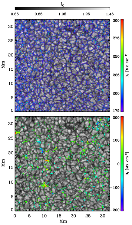
Figure 1.— Snapshot of the solar surface (i.e. granulation) as seen by IMaX. Gray-scale corresponds to the normalized continuum intensity. Colors correspond to $B_{\parallel}$ and $B_{\perp}$ on the bottom and top panels respectively. Only those pixels where the magnetic flux is at least three times the standard deviation are plotted.

The reduction procedure renders time series of ${\bf S}(\lambda)$ with a cadence of $\Delta t=33$ sec; a spatial sampling of 0$\farcs$055 per pixel, and an effective field-of-view of 45″$\times$45″. The total number of available images is $T=113$, yielding a total observing time of $62$ minutes.

From here we infer the longitudinal $B_{\parallel}$ and transverse $B_{\perp}$ magnetic field flux density at each pixel on the detector using an inversion method based on the radiative transfer equation for the Stokes parameters by means the VFISV code Borrero et al. (2011), which assumes that the physical parameters of the atmosphere model (except for the source function) are constant along the vertical direction in the solar atmosphere within the range of optical-depths where this spectral line is formed (i.e. Milne-Eddington approximation). Following Graham et al. (2002) we refer to $B_{\parallel}$ and $B_{\perp}$ as the magnetic flux density through surfaces whose normal vectors are oriented parallel and perpendicularly, respectively, to the line-of-sight.

The signal-to-noise ratio of the observations is affected by: the Poisson photon noise of the instrument, accuracy of the polarimetric calibration and quantum efficiency of the detectors. Following Borrero & Kobel (2011) we have estimated a standard deviation of components $\sigma_{\parallel}\approx 8$ Mx cm^-2 and $\sigma_{\perp}\approx 55$ Mx cm^-2 as a measure of our accuracy in the determination of the magnetic field density components.

Figure 1 shows a snapshot of the solar surface (i.e. quiet Sun granulation) as seen by IMaX. We also overplot the retrieved values of $B_{\parallel}$ (bottom panel) and $B_{\perp}$ (top panel, but only in those pixels where the inferred values are about three times above the standard deviation: $|B_{\parallel}|\gtrsim 25$ Mx cm^-2 and $B_{\perp}\gtrsim 175$ Mx cm^-2.

3. Data analysis

In this section, we present a brief theoretical overview on Markov random variables (Sect. 3.1) and demonstrate how Markov property has been analyzed and confirmed in our observational data (Sect. 3.2).

3.1. Markov property: theory

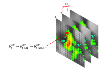
Figure 2.— Geometry (schematic, not to scale) of the analyzed fluctuations. Image pixels (red square) define a spatial uniform grid at whose nodes we register occurrences (above the noise level) of the observable $b^{xy}_{t}$ in time (see Eq.(5)). The sequences (chains) at each spatial pixel have finite lengths due to interruption by noise and apparent motion of the magnetic concentrations. For the Markov property test, all chains we part into time-ordered pairs and triplets of the random samples (see Eq.(3), Eq.(4) and Fig.3). All pixels are considered to be spatially independent contributors across the entire field-of-view to the single set of the registered chains.

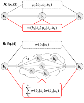
Figure 3.— Schematic representation of the necessary and sufficient conditions for the Markov property: chart A corresponds to Eq.(3) and chart B to Eq.(4). Algebraic relations in Eq.(3)-(4) between statistical quantities are verified by comparison of the independently estimated right-hand side (dotted blocks) and corresponding left-hand side (solid line blocks) of each equation (see text for rigorous definitions and Fig.4 for results). Statistic is collected from a set of time-ordered (arrows) pairs and triplets of the random realizations $\{b_{1},b_{2},b_{3}\}$ (see Eq.(5) and Section 3.2), which in turn are acquired as shown in Fig.2. Lines connecting formulae blocks and $b_{1,2,3}$-values show dependence of the functions on their arguments. The red blocks designate estimated functions shown with red lines in Fig.4, and dotted blocks correspond to the circles in Fig.4.

Consider a time-discrete stochastic process $b(t)$, the random variable $b$ is defined over a finite set of discrete states (state space). The state space has $\mathcal{M}$ distinct elements.

Let $p_{n}({b_{n},t_{n};\ldots;b_{1},t_{1}})\equiv p_{n}({b_{n}\ldots b_{1}})$ be the $n$-joint probability density function (pdf) such that $p_{n}(b_{n}\ldots b_{1})d^{n}b$ is the probability that $b$ has values in the interval $[b_{1},b_{1}+db)$ at time $t_{1}$, …and in the range $[b_{n},b_{n}+db)$ at time instance $t_{n}$. For brevity, the intervals are labeled by the representative states, that is to say that the process $b(t)$ is in the state $b_{m}$ at time $t_{m}$ if the random variable $b$ has values in $[b_{m},b_{m}+db)$ at time $t_{m}$. Empirically, $db$ is the fixed binsize that has been introduced for the estimation of the probabilities, and it is henceforth neglected in the equations for simplicity. Some trivial properties of the probabilities are $0\leq p(b)db\leq 1$ and $\sum_{b}^{\mathcal{M}}p(b)db=1$ with $p_{1}(b)\equiv p(b)$.

The conditional probability density function $w_{n}({b_{n}|b_{n-1}\ldots b_{1}})$ is defined such that $w_{n}$ is the probability for $b(t)$ to be in state $b_{n}$ at time $t_{n}$ if the random variable $b$ already passed through the states $b_{n-1}\ldots b_{1}$ at later times $[t_{n-1},t_{1}]$, which we call a history of the process $\mathcal{H}\equiv b_{n-1}\ldots b_{1}$. By definition:

$$w_{n}({b_{n}|\mathcal{H}})=p_{n}({b_{n}\ldots b_{1}})/p_{n-1}({\mathcal{H}})\;.$$ (1)

A time- and space-discrete stochastic process $b(t)$ is a called Markov chain (e.g. Oppenheim et al., 1977) if the history of the process $\mathcal{H}$ can be reduced to a single state, which is assigned to be immediately preceding the current one:

$$w_{n}({b_{n}|\mathcal{H}})=w({b_{n}|b_{n-1}})\;.$$ (2)

It is worth mentioning that $p_{n-1}$ and $p_{n}$ are functions of $n-1$ and $n$ independent variables being represented by $\mathcal{M}^{n-1}$ and $\mathcal{M}^{n}$ state configurations, respectively. Due to the moderate size of the dataset we set $n=3$ in Eq.(1) (see also Friedrich & Peinke, 1997; Friedrich et al., 2011) and obtain the following equation describing the first condition of the Markov property:

$$p_{3}({b_{3},b_{2},b_{1}})=w({b_{3}|b_{2}})p_{2}({b_{2},b_{1}})\;.$$ (3)

The second condition we examine is based on the integral form of the Chapman-Kolmogorov equation (e.g. van Kampen, 1992), which reflects the time ordering of the chain:

$$w({b_{3}|b_{1}})=\sum_{b_{2}}^{\mathcal{M}}w({b_{3}|b_{2}})w({b_{2}|b_{1}})\;,$$ (4)

where each $w$ is a $\mathcal{M}^{2}$ transition matrix. On their own Eq.(3) and Eq.(4) are necessary conditions for a stochastic process to have the Markov property, while together they represent also a sufficient condition (see Fuliński et al., 1998, and references therein). Therefore, in the following, these two conditions are used simultaneously in order to test for the Markov property of the observed fluctuations in $B_{\parallel}$, $B_{\perp}$, and $B^{2}$ (see Eq.(5)).

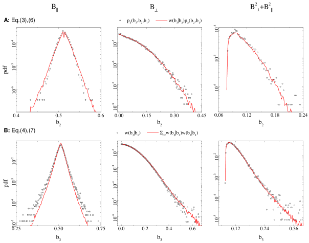
Figure 4.— The results of the Markov property test. The vertical arrangement of panels corresponds to three analyzed observables. Top row A: test of the relation given by Eq.(8). Bottom row B: test of the relation given by Eq.(9). The abscissa axes are shown in normalized values (dimensionless). The observables $B_{{\sc XXX}}$ are linearly normalized into continuum interval $b\in[0,1]$ according to $b=(B_{\sc XXX}-B_{min})/(B_{max}-B_{min})$, where the global extreme values $B_{min}$ and $B_{max}$ are estimated during the pixel selection procedure (for double transitions) over all $T$ images. For $B_{||}$, the empty noise cutoff range $[-3\sigma_{||},3\sigma_{||})$ is removed during the normalization procedure.

3.2. Markov property: test

It has been shown by Asensio Ramos (2009) that spatial increment $h_{r}(x,y)=B_{\perp}(x+r,y+r)-B_{\perp}(x,y)$ does not show Markov properties, where $B_{\perp}(x,y)$ is the line-of-sight magnetic flux density (see Section 2) registered at pixel $(x,y)$ and $B_{\perp}(x+r,y+r)$ is the same quantity but separated by the distance (spatial scale) $r$. In this paper we perform a similar Markov analysis to the aforementioned work but in the time domain and for the observables themselves, not their increments: we examine Markov properties of transitions/fluctuation of the observable $b^{xy}_{t}$ in time (from image to image) at a given pixel:

$$b^{xy}_{t}\rightarrow b^{xy}_{t+\Delta t}\rightarrow b^{xy}_{t+2\Delta t}\cdots\;,$$ (5)

where $\Delta t$ is the cadence time (Section 2), and $b^{xy}$ is one of three variables ($B_{\perp},B_{||},B^{2}$) inferred at image pixel $(x,y)$. A relation between observable, image pixel(s) and cadence time is schematically shown in Fig.2.

The Markov property is tested by comparing the independently estimated left- and right-hand sides of Eq.(3) and Eq.(4) (see scheme in Fig.3). That is, we count the number of occurrences of the pairs (single transitions) for $p_{2}(b^{xy}_{t+\Delta t},b^{xy}_{t})$ and $w(b^{xy}_{t+\Delta t}|b^{xy}_{t})$ and triplets (double transitions) for $p_{3}(b^{xy}_{t+2\Delta t},b^{xy}_{t+\Delta t},b^{xy}_{t})$ according to Eq.(5). In Fig.3, the red blocks designate estimated functions shown with red lines in Fig.4. The dotted blocks in Fig.3 correspond to the circles in Fig.4.

In order to determine the statistics of the transitions described by Eq.(5) we analyze only those pixels where the signal is above the $3\sigma$-noise cut-off simultaneously at $t$ and $t+\Delta t$ at the same spatial location $(x,y)$. This is done for all conditional probability functions $w$ and the two-joint probability function $p_{2}({b_{2},b_{1}})$ in Eq.(3) and Eq.(4). Likewise, for the three-joint probability function $p_{3}({b_{3},b_{2},b_{1}})$ in Eq.(3) the condition is that the signal must be above the $3\sigma$ cut-off in three images at $t,t+\Delta t$ and $t+2\Delta t$. Such pixel-wise analysis of images makes the notion of extended magnetic feature to be irrelevant, as well as their tracking.

The explicit computation of Eq.(3) reveals that the range of values in which $p_{3}$ is defined, given by the $\mathcal{M}^{3}$-dimensional space of independent samples, is quite sparse. Thus, in order to improve its statistical significance, we select those triples that have maximal occurrence in the $\mathcal{M}^{3}$-space and those with occurrence value of at least 90% of the maximal one. We refer to the set of statistically reliable points as $(b^{\prime}_{3},b^{\prime}_{2},b^{\prime}_{1})$.

The test of the Markov property is split into two steps. First, we transform $p_{3}$, $p_{2}$ and $w$ into $\mathcal{M}$-dimensional vectors by fixing the variables $b_{3}$ and $b_{1}$ to each of those points selected as statistically reliable: $b_{3}=b^{\prime}_{3}$ and $b_{1}=b^{\prime}_{1}$:

(7)

such that they transform Eq.(3) into an identity with respect to the free variable $b_{2}$:

$$p_{3}(b_{2})|_{b^{\prime}_{3},b^{\prime}_{1}}=w(b_{2})|_{b^{\prime}_{3}}p_{2}(b_{2})|_{b^{\prime}_{1}}$$ (8)

and Eq.(4) into $\mathcal{M}$-vector function of the free variable $b_{3}$.

$$w(b_{3})|_{b^{\prime}_{1}}=\sum_{b_{2}}w(b_{3}|b_{2})w(b_{2})|_{b^{\prime}_{1}}\;.$$ (9)

To further increase the statistics, a second step in our test of the Markov property consists in averaging the left- and right- hand sides of Eq.(8) and Eq.(9) for all primed points that were previously selected.

The results of the described procedure are shown in Fig.4. The top row panels in Fig.4 show the estimated relation corresponding to Eq.(8) and bottom panels to Eq.(9). Circles represent the estimated left-hand sides of both equations, while the solid lines correspond to the right-hand sides. From these figures it can be concluded that, around the global and a few of local maxima of the $\mathcal{M}^{3}$-space, the Markov property is clearly satisfied.

4. Conclusions

Stochastic Markov processes are intermediate processes that lie between pure randomness of the independent events and those processes with a strong dependence on the past states (i.e. history) (e.g. Oppenheim et al., 1977).

Our analysis establishes that the magnetic field temporal fluctuations, as seen by IMaX with a resolution of 0.15″-0.18″and $33$ sec cadence, can be considered as a Markov discrete stochastic process (Markov chain). The sufficient and necessary conditions for the Markov processes have been verified for the case of the maxima (global and local) of the available statistics.

The revealed Markov property in the temporal dynamics of the turbulent small-scale magnetic field is the quiet Sun can be used to constraint magneto-hydrodynamics models of the solar atmosphere and a stellar turbulent dynamo, in general. That is to say, the Markov property should be reproducible in the relevant simulations of the photospheric magnetic fields.

With this work we hope to have brought forward new ideas and techniques for the analysis of solar spectropolarimetric data. We foresee a number of future applications of the method described in this paper. For instance, in a future work we plan to investigate the so-called Markov-Einstein time-scale. This time scale is the minimum time interval over which the stochastic data can be considered as a Markov process. On shorter time scales, one expects to find correlations and thus memory effects start to play a significant role in transition probabilities (Friedrich et al., 2011, and references therein). The cadence $\Delta t$ in our data seems to be greater than (or just equal to) the Markov-Einstein time-scale for the spatial resolution of our observations. To have an exact relation between temporal/spatial resolution and Markov property, one needs to perform a systematic analysis of similar observations with different resolutions and cadences. This will be the subject of a future investigation.

This work was supported by the European Research Council Advanced Grant HotMol (ERC-2011-AdG 291659). We are grateful to Prof. Udo Seifert for useful comments and suggestions. We thank anonymous referee for valuable comments that helped to clarify and improve the paper substantially. This research has made use of NASA’s Astrophysics Data System.

Facilities: SUNRISE/IMaX

References

- Arge & Pizzo (2000) Arge, C. N., & Pizzo, V. J. 2000, J. Geophys. Res., 105, 10465
- Asensio Ramos (2009) Asensio Ramos, A. 2009, A&A, 494, 287
- Barthol et al. (2011) Barthol, P., Gandorfer, A., Solanki, S. K., et al. 2011, Sol. Phys., 268, 1
- Berkefeld et al. (2011) Berkefeld, T., Schmidt, W., Soltau, D., et al. 2011, Sol. Phys., 268, 103
- Borrero & Kobel (2011) Borrero, J. M., & Kobel, P. 2011, A&A, 527, A29
- Borrero et al. (2011) Borrero, J. M., Tomczyk, S., Kubo, M., et al. 2011, Sol. Phys., 273, 267
- Cohen et al. (2007) Cohen, O., Sokolov, I. V., Roussev, I. I., et al. 2007, ApJ, 654, L163
- DeForest et al. (2007) DeForest, C. E., Hagenaar, H. J., Lamb, D. A., Parnell, C. E., & Welsch, B. T. 2007, ApJ, 666, 576
- Friedrich & Peinke (1997) Friedrich, R., & Peinke, J. 1997, Physical Review Letters, 78, 863
- Friedrich et al. (2011) Friedrich, R., Peinke, J., Sahimi, M., & Tabar, M. R. R. 2011, Physics Reports, 506, 87
- Fuliński et al. (1998) Fuliński, A., Grzywna, Z., Mellor, I., Siwy, Z., & Usherwood, P. N. R. 1998, Phys. Rev. E, 58, 919
- Graham et al. (2002) Graham, J. D., López Ariste, A., Socas-Navarro, H., & Tomczyk, S. 2002, Sol. Phys., 208, 211
- Hagenaar et al. (2012) Hagenaar, H., Shine, R., Ryutova, M., & Dalda, A. S. 2012, in Astronomical Society of the Pacific Conference Series, Vol. 454, Hinode-3: The 3rd Hinode Science Meeting, ed. T. Sekii, T. Watanabe, & T. Sakurai, 181
- Iida et al. (2012) Iida, Y., Hagenaar, H. J., & Yokoyama, T. 2012, ApJ, 752, 149
- Knuth (2006) Knuth, K. H. 2006, ArXiv Physics e-prints
- Lamb et al. (2008) Lamb, D. A., DeForest, C. E., Hagenaar, H. J., Parnell, C. E., & Welsch, B. T. 2008, ApJ, 674, 520
- Lamb et al. (2010) Lamb, D. A., DeForest, C. E., Hagenaar, H. J., Parnell, C. E., & Welsch, B. T. 2010, The Astrophysical Journal, 720, 1405
- Lamb et al. (2013) Lamb, D. A., Howard, T. A., DeForest, C. E., Parnell, C. E., & Welsch, B. T. 2013, ApJ, 774, 127
- Longcope & Kankelborg (1999) Longcope, D. W., & Kankelborg, C. C. 1999, ApJ, 524, 483
- Martínez Pillet et al. (2011) Martínez Pillet, V., Del Toro Iniesta, J. C., Álvarez-Herrero, A., et al. 2011, Sol. Phys., 268, 57
- Oppenheim et al. (1977) Oppenheim, I., Shuler, K. E., & Weiss, G. H. 1977, Stochastic processes in chemical physics : the master equation (MIT Press)
- Parnell (2001) Parnell, C. E. 2001, Sol. Phys., 200, 23
- Parnell et al. (2009) Parnell, C. E., DeForest, C. E., Hagenaar, H. J., et al. 2009, ApJ, 698, 75
- Schrijver et al. (1997) Schrijver, C. J., Title, A. M., van Ballegooijen, A. A., Hagenaar, H. J., & Shine, R. A. 1997, ApJ, 487, 424
- Solanki et al. (2006) Solanki, S. K., Inhester, B., & Schüssler, M. 2006, Reports on Progress in Physics, 69, 563
- Solanki et al. (2010) Solanki, S. K., Barthol, P., Danilovic, S., et al. 2010, The Astrophysical Journal Letters, 723, L127
- Stenflo (2013) Stenflo, J. O. 2013, A&A Rev., 21, 66
- Thornton & Parnell (2011) Thornton, L., & Parnell, C. 2011, Solar Physics, 269, 13
- Uritsky et al. (2013) Uritsky, V. M., Davila, J. M., Ofman, L., & Coyner, A. J. 2013, ApJ, 769, 62
- van Kampen (1992) van Kampen, N. G. 1992, Stochastic Processes in Physics and Chemistry
- Wiegelmann et al. (2015) Wiegelmann, T., Neukirch, T., Nickeler, D. H., et al. 2015, ApJ, 815, 10
- Wiegelmann et al. (2013) Wiegelmann, T., Solanki, S. K., Borrero, J. M., et al. 2013, Sol. Phys., 283, 253