Friedmann dynamics recovered from compactified Einstein-Gauss-Bonnet cosmology

Abstract

In this paper cosmological dynamics in Einstein-Gauss-Bonnet gravity with a perfect fluid source in arbitrary dimension is studied. A systematic analysis is performed for the case that the theory does not admit maximally symmetric solutions. Considering two independent scale factors, namely one for the three dimensional space and one for the extra dimensional space, is found that a regime exists where the two scale factors tend to a constant value via damped oscillations for not too negative pressure of the fluid, so that asymptotically the evolution of the $(3+1)$-dimensional Friedmann model with perfect fluid is recovered. At last, it is worth emphasizing that the present numerical results strongly support a ’t Hooft-like interpretation of the parameter $1/D$ (where $D$ is the number of extra dimensions) as a small expansion parameter in very much the same way as it happens in the large $N$ expansion of gauge theories with $1/N$. Indeed, the dependence on $D$ of many of the relevant physical quantities computed here manifests a clear WKB-like pattern, as expected on the basis of large $N$ arguments.

I Introduction

One of the outstanding conceptual features of General Relativity (GR) is that the geometry of space-time itself is a dynamical object. This opens the possibility that there may exist more than three space dimensions which are not observable because they may be compactified to a very small scale. This idea was implemented the first time by Kaluza KK1 and Klein KK2 ; KK3 assuming one extra space dimensions in order to attempt to unify gravity with electromagnetism. This idea can be extended to include non-Abelian gauge fields by introducing more extra dimensions. Moreover the existence of extra dimensions is also predicted by String Theory. The low energy sector of some String theories is not described by General Relativity but by a generalization of it known in literature as Einstein-Gauss-Bonnet gravity (see e.g. GastGarr ). The action of this theory is the sum of three terms two of which are the familiar $\Lambda$-term and the Einstein-Hilbert term whereas the third term is the Gauss-Bonnet term which is quadratic in the curvature and reads $I_{GB}=\int\sqrt{-g}(R^{2}-4R_{\mu\nu}R^{\mu\nu}+R_{\alpha\beta\mu\nu}R^{\alpha\beta\mu\nu})$. In four dimension the Gauss-Bonnet term is topological and does not affect the equations of motion. In dimension higher than four however this term leads to a non-trivial contribution to equation of motion. As this non-trivial contribution is still of second order in the derivatives of the metric, Einstein-Gauss-Bonnet gravity can be considered as a natural extension of General Relativity to higher dimensions as its action is constructed according to the same principles as the Einstein Hilbert action in four dimensions. Einstein-Gauss-Bonnet gravity is actually a particular case of a more general gravity theory known as Lovelock gravity Lovelock . In the same way as the Gauss-Bonnet term, which is topological in four dimensions but gives a non-trivial contribution to the equations of motion in higher dimension in every odd dimension it is possible to add a new higher power term in the curvature which is topological in the lower even dimension (this means for example that in seven dimensions the most generic Lovelock theory is sum of four terms namely the three terms of Einstein-Gauss-Bonnet gravity and a new term which is cubic the curvature). All these higher power terms again lead to a non-trivial contribution to the equations of motion which is of second order in the derivatives.

Even if Lovelock gravity is constructed according to the same principles as General Relativity it has some features which are absent in General Relativity. For example in the first order formalism the equation of motion do not imply the vanishing of torsion TZ-CQG which therefore becomes a new propagating degree of freedom. Exact solution with non-trivial vacuum torsion have been found in CGT07 ; CGW07 ; CG ; CG2 ; ACGO . In this paper however we will consider the zero torsion sector.

Perhaps one of the most new feature of Lovelock gravity is that the “Lambda term” in the action is not directly related to the cosmological constant in the sense that it does not measure the curvature of the maximally symmetric solution. Actually for a $N$th order Lovelock theory there can exist up to to $N$ different maximally symmetric solutions where the curvature radii are function of all Lovelock couplings. A very peculiar case happens when the highest Lovelock term in the action is of even power in the curvature as there may exist no maximally symmetric solution at all so that the vacuum state must be necessarily a less symmetric space-time. This situation can be interpreted as a case of “geometric frustration” (see e.g. CGP1 ; CGP2 ).

In order to recover physics in four space-time dimensions it is necessary to check if the equations of motion of Lovelock gravity admit compactified solutions known in literature as “spontaneous compactification”. Exact static solutions where the metric is a cross product of a (3+1)-dimensional manifold and a constant curvature “inner space”, were discussed for the first time in add_1 , but with (3+1)-dimensional manifold being actually Minkowski (the generalization for a constant curvature Lorentzian manifold was done in Deruelle2 ). It was shown in CGTW09 that in order to recover four dimensional General Relativity with arbitrarily small cosmological constant and with arbitrarily small static extra dimensions it is necessary to have a Lovelock theory which includes also at least a cubic term so that the minimal space-time dimension where such a spontaneous compactification can happen is seven.

In the context of cosmology it is of course of fundamental interest to consider a spontaneous compactification where the four dimensional part is given by a Friedmann-Robertson-Walker metric. In this case it is then completely natural to consider also the size of the extra dimensions as time dependent rather then static. Indeed in add_4 it was explicitly shown that in order to have a more realistic model one needs to consider the dynamical evolution of the extra dimensional scale factor as well. In Deruelle2 the equations of motion for compactification with both time dependent scale factors were written for arbitrary Lovelock order in the special case that both factors are flat. The results of Deruelle2 were reanalyzed for the special case of 10 space-time dimensions in add_10 . In add_8 the existence of dynamical compactification solutions was studied with the use of Hamiltonian formalism. More recently efforts in finding spontaneous compactifications have been done in add13 where the dynamical compactification of (5+1) Einstein-Gauss-Bonnet (EGB) model was considered, in MO04 ; MO14 with different metric ansatz for scale factors corresponding to (3+1)- and extra dimensional parts, and in CGP1 ; CGP2 where general (e.g. without any ansatz) scale factors and curved manifolds were considered. Also, apart from cosmology recent analysis focuses on properties of black holes in Gauss-Bonnet addn_1 ; addn_2 and Lovelock addn_3 ; addn_4 gravities, features of gravitational collapse in these theories addn_5 ; addn_6 ; addn_7 , general features of spherical-symmetric solutions addn_8 and many others.

The most common ansatz used to find exact solutions for the functional form of the scale factor were exponentials or power laws. Exact solutions with exponential functions for both the (3+1)- and extra dimensional scale factors were studied the first time in Is86 and exponentially increasing (3+1)-dimensional scale factor and exponentially shrinking extra dimensional scale factor were described. Power-law solutions have been analyzed in Deruelle1 ; Deruelle2 and more recently mpla09 ; prd09 ; Ivashchuk ; prd10 ; grg10 so that there is an almost complete description (see also PT for useful comments regarding physical branches of the solutions). More recently solutions with exponential scale factors KPT have been studied in detail namely models with both variable CPT1 and constant CST2 volume developing a general scheme for constructing solutions in EGB; recently CPT3 this scheme was generalized for general Lovelock gravity of any order and in any dimensions as well. Also, the stability of the solutions was addressed in my15 , where it was demonstrated that only a handful of the solutions could be called “stable” while the remaining are either unstable or have neutral/marginal stability and so additional investigation is required.

In order to find all possible regimes of Einstein-Gauss-Bonnet cosmology it is necessary to go beyond an exponential or power law ansatz and keep the functional form of the scale factor generic. In this case the equations of motion are too difficult to be solved analytically and so a numerical analysis must be performed. In CGP1 it was found that there exist a phenomenologically sensible regime in the case that the curvature of the extra dimensions is negative and the Einstein-Gauss-Bonnet theory does not admit a maximally symmetric solution. In this case the three dimensional Hubble parameter and the extra dimensional scale factor tend to constant values asymptotically. Due to the fact that the theory does not admit maximally symmetric solution the compactification was interpreted as geometric frustration. The reduced symmetry vacua of a Lovelock theory without maximally symmetric solution have been explored in castor_2015 . In CGP2 a detailed analysis of the cosmological dynamics of Einstein-Gauss-Bonnet gravity with generic couplings was performed. In most cases it turned out that there exist non-physical features like a finite time future singularity or isotropization. The only situation where a realistic dynamics could be achieved turned out to be the case when the theory does not admit maximally symmetric solutions (and with negative curvature of the extra dimensions).

A further benefit to use two different scale factors for the three “macroscopic” dimensions and the $D$ extra-dimensions is that it allows to disclose a clear “large $N$ pattern” in the dependence of relevant physical observables on the number of extra-dimensions. In gauge theories the large $N$ expansions introduced by ’t Hooft in thooft (and generalized by Veneziano in veneziano to take into account the presence of matter fields in the fundamental) provides with a very clever small parameter suitable to generate an alternative perturbative expansion (namely $1/N$) which does not necessarily require the theory to be weakly coupled. A crucial step to achieve this goal is to separate in a very clear way the dependence on internal indices from the dependence on “space-time” indices of all relevant quantities (for two nice reviews see MAKMAN ). Such large $N$ expansion is very closely related to the semi-classical or WKB expansion and is a very powerful non-perturbative tool in field theory. In (3+1) dimensional General Relativity the situation is complicated by the fact that it is not easy to distinguish “internal” from “space-time” indices in the second order formalism (in the first order formalism the results in canfora2005 suggest that the ’t Hooft expansion in gravity in (3+1) dimensions has many features absent in the Yang-Mills case). However, in the case of Kaluza-Klein theories, there is a parameter which is clearly analogous to the ’t Hooft parameter $N$: the number of extra dimensions CGZ . The results of the present paper clearly suggest that the same is true for EGB theory. For this reason, the field equations have been written in order to display explicitly the dependence on $D$. The present analysis shows that the dependence of many relevant quantities on the number of extra dimensions exhibit a WKB-like pattern.

Of course in cosmology it is also crucial to study the effect of a matter source on the cosmological dynamics. For this reason the purpose of this paper is to explore the effect of a perfect fluid on Einstein-Gauss-Bonnet cosmology in the geometric frustration regime. Especially the emergence of new subregimes is studied. It is found that there exist a new subregime where both scale factors tend to constant values by performing damped oscillations so that the Friedmann dynamics can be recovered asymptotically. It is also worth to point out that the dependence of the relevant physical quantities on the number of the extra-dimensions reminds very closely what one would expect from a large $N$ expansion in gauge theories in which the number of extra-dimensions plays the role of $N$ in the ’t Hooft expansion. In particular, the present analysis discloses a clear eikonal-like pattern.

The structure of the paper will be the following: in section 2, some analytic considerations are given of why it is necessary to consider the geometric frustration regime. In section 3, the subregime which can recover $(3+1)$-dimensional Friedmann model is introduced. In section 4 matter is added and the numerical analysis is performed. Section 5 is dedicated to the conclusions.

II Equations of motion

Lovelock gravity Lovelock has the following structure: its Lagrangian is constructed from terms

$$L_{n}=\frac{1}{2^{n}}\delta^{i_{1}i_{2}\dots i_{2n}}_{j_{1}j_{2}\dots j_{2n}}R^{j_{1}j_{2}}_{i_{1}i_{2}}\dots R^{j_{2n-1}j_{2n}}_{i_{2n-1}i_{2n}},$$ (1)

where $\delta^{i_{1}i_{2}\dots i_{2n}}_{j_{1}j_{2}\dots j_{2n}}$ is the generalized Kronecker delta of the order $2n$. One can verify that $L_{n}$ is Euler invariant in $D<2n$ spatial dimensions and so it would not give nontrivial contribution into the equations of motion. So that the Lagrangian density for any given $D$ spatial dimensions is sum of all Lovelock invariants (1) upto $n=\left[\displaystyle\frac{D}{2}\right]$ which give nontrivial contributions into equations of motion:

$${\cal L}=\sqrt{-g}\sum_{n}c_{n}L_{n},$$ (2)

where $g$ is the determinant of metric tensor, $c_{n}$ is a coupling constant of the order of Planck length in $2n$ dimensions and summation over all $n$ in consideration is assumed.

The ansatz for the metric is

$$ds^{2}=-dt^{2}+a(t)^{2}d\Sigma_{(3)}^{2}+b(t)^{2}d\Sigma_{(\mathbf{D})}^{2}\ ,$$ (3)

where $d\Sigma_{(3)}^{2}$ and $d\Sigma_{(\mathbf{D})}^{2}$ stand for the metric of two constant curvature manifolds $\Sigma_{(3)}$ and $\Sigma_{(\mathbf{D})}$. It is worth to point out that even a negative constant curvature space can be compactified by making the quotient of the space by a freely acting discrete subgroup of $O(D,1)$ wolf .

The complete derivation of the equations of motion could be found in our previous papers, dedicated to the description of the particular regime which appears in this model CGP1 ; CGP2 . For simplicity we consider the case with $\gamma_{\left(3\right)}=0$ (zero spatial curvature for “our” (3+1)-dimensional world; nonzero $\gamma_{\left(3\right)}$ does not affect the presence of the dynamical compactification regime, as discussed in CGP1 ; CGP2 ). For the moment the non-zero curvature for extra dimensions can be normalized as $\gamma_{\left(\mathbf{D}\right)}=\pm 1$. Since there is no curvature term for $a(t)$, it is useful to rewrite the equations of motion in terms of the Hubble parameter $H(t)=\dot{a}(t)/a(t)$; the equations will take a form

$$\begin{array}[]{l}\displaystyle\frac{(D+3)(D+2)(D+1)}{6}c_{0}+\displaystyle\frac{(D+1)D(D-1)}{6}c_{1}\left[\displaystyle\frac{\gamma_{\left(\mathbf{D}\right)}+\dot{b}(t)^{2}}{b(t)^{2}}+\displaystyle\frac{6H(t)\dot{b}(t)}{b(t)(D-1)}+\displaystyle\frac{6H(t)^{2}}{D(D-1)}\right]+\\ \\ +\displaystyle\frac{(D-1)(D-2)(D-3)}{6}c_{2}\left[\displaystyle\frac{(\gamma_{\left(\mathbf{D}\right)}+\dot{b}(t)^{2})^{2}}{b(t)^{4}}+\displaystyle\frac{12H(t)^{2}(\gamma_{\left(\mathbf{D}\right)}+\dot{b}(t)^{2})}{b(t)^{2}(D-2)(D-3)}+\displaystyle\frac{24H(t)^{2}\dot{b}(t)^{2}}{b(t)^{2}(D-2)(D-3)}+\right.\\ \\ \left.+\displaystyle\frac{12(\gamma_{\left(\mathbf{D}\right)}+\dot{b}(t)^{2})H(t)\dot{b}(t)}{b(t)^{3}(D-3)}+\displaystyle\frac{24H(t)^{3}\dot{b}(t)}{b(t)(D-1)(D-2)(D-3)}\right]=0,\end{array}$$ (4)

$$\begin{array}[]{l}\displaystyle\frac{(D+3)(D+2)(D+1)}{6}c_{0}+\displaystyle\frac{(D+1)D(D-1)}{6}c_{1}\left[\displaystyle\frac{\gamma_{\left(\mathbf{D}\right)}+\dot{b}(t)^{2}}{b(t)^{2}}+\displaystyle\frac{4(\dot{H}(t)+H(t)^{2})}{D(D-1)}+\displaystyle\frac{2\ddot{b}(t)}{b(t)(D-1)}+\right.\\ \\ \left.+\displaystyle\frac{2H(t)^{2}}{D(D-1)}+\displaystyle\frac{4H(t)\dot{b}(t)}{b(t)(D-1)}\right]+\displaystyle\frac{(D-1)(D-2)(D-3)}{6}c_{2}\left[\displaystyle\frac{(\gamma_{\left(\mathbf{D}\right)}+\dot{b}(t)^{2})^{2}}{b(t)^{4}}+\right.\\ \\ \left.+\displaystyle\frac{16(\dot{H}(t)+H(t)^{2})H(t)\dot{b}(t)}{b(t)(D-1)(D-2)(D-3)}+\displaystyle\frac{8(\gamma_{\left(\mathbf{D}\right)}+\dot{b}(t)^{2})H(t)\dot{b}(t)}{b(t)^{3}(D-3)}+\displaystyle\frac{8(\dot{H}(t)+H(t)^{2})(\gamma_{\left(\mathbf{D}\right)}+\dot{b}(t)^{2})}{b(t)^{2}(D-2)(D-3)}+\right.\\ \\ \left.+\displaystyle\frac{8H(t)^{2}\ddot{b}(t)}{b(t)(D-1)(D-2)(D-3)}+\displaystyle\frac{16\ddot{b}(t)H(t)\dot{b}(t)}{b(t)^{2}(D-2)(D-3)}+\displaystyle\frac{4\ddot{b}(t)(\gamma_{\left(\mathbf{D}\right)}+\dot{b}(t)^{2})}{b(t)^{3}(D-3)}+\right.\\ \\ \left.+\displaystyle\frac{4H(t)^{2}(\gamma_{\left(\mathbf{D}\right)}+\dot{b}(t)^{2})}{b(t)^{2}(D-2)(D-3)}+\displaystyle\frac{8H(t)^{2}\dot{b}(t)^{2}}{b(t)^{2}(D-2)(D-3)}\right]=0,\end{array}$$ (5)

$$\begin{array}[]{l}\displaystyle\frac{D(D+3)(D+2)(D+1)}{6}c_{0}+\displaystyle\frac{(D-2)(D+1)D(D-1)}{6}c_{1}\left[\displaystyle\frac{\gamma_{\left(\mathbf{D}\right)}+\dot{b}(t)^{2}}{b(t)^{2}}+\displaystyle\frac{6(\dot{H}(t)+H(t)^{2})}{(D-2)(D-1)}+\right.\\ \\ \left.\displaystyle\frac{2\ddot{b}(t)}{b(t)(D-2)}+\displaystyle\frac{6H(t)^{2}}{(D-2)(D-1)}+\displaystyle\frac{6H(t)\dot{b}(t)}{b(t)(D-2)}\right]+\displaystyle\frac{(D-1)(D-2)(D-3)}{6}c_{2}\times\\ \\ \times\left[\displaystyle\frac{(\gamma_{\left(\mathbf{D}\right)}+\dot{b}(t)^{2})^{2}}{b(t)^{4}}(D-4)+\displaystyle\frac{48(\dot{H}(t)+H(t)^{2})H(t)\dot{b}(t)}{b(t)(D-2)(D-3)}+\displaystyle\frac{12(\gamma_{\left(\mathbf{D}\right)}+\dot{b}(t)^{2})H(t)\dot{b}(t)}{b(t)^{3}}+\right.\\ \\ \left.+\displaystyle\frac{24H(t)^{2}\dot{b}(t)^{2}}{b(t)^{2}(D-3)}+\displaystyle\frac{12(\dot{H}(t)+H(t)^{2})(\gamma_{\left(\mathbf{D}\right)}+\dot{b}(t)^{2})}{b(t)^{2}(D-3)}+\displaystyle\frac{24H(t)^{2}\ddot{b}(t)}{b(t)(D-2)(D-3)}+\displaystyle\frac{24\ddot{b}(t)H(t)\dot{b}(t)}{b(t)^{2}(D-3)}+\right.\\ \\ \left.+\displaystyle\frac{4\ddot{b}(t)(\gamma_{\left(\mathbf{D}\right)}+\dot{b}(t)^{2})}{b(t)^{3}}+\displaystyle\frac{12H(t)^{2}(\gamma_{\left(\mathbf{D}\right)}+\dot{b}(t)^{2})}{b(t)^{2}(D-3)}+\displaystyle\frac{24H(t)^{3}\dot{b}(t)}{b(t)(D-2)(D-3)}+\displaystyle\frac{24(\dot{H}(t)+H(t)^{2})H(t)^{2}}{(D-1)(D-2)(D-3)}\right]=0,\end{array}$$ (6)

as $\mathcal{E}_{0}=0$ equation (4), $\mathcal{E}_{i}=0$ (5), and $\mathcal{E}_{a}=0$ (6). In CGP1 ; CGP2 we described a regime which naturally appear if a choice for coupling constants forbids existence of maximally-symmetric solutions. A maximally symmetric space-time has curvature two form given by

$$R^{AB}=\Lambda_{D+4}e^{A}e^{B},$$ (7)

which inserted in the equations of motion gives a quadratic equation for $\Lambda_{D+4}$:

$$(c_{2}\Lambda_{D+4}^{2}+c_{1}\Lambda_{D+4}+c_{0})e^{A_{1}}\ldots e^{A_{D+4}}=0,$$ (8)

which admits as solutions

$$\Lambda_{eff}\equiv\Lambda_{D+4}=\frac{-c_{1}\pm\sqrt{(c_{1})^{2}-4c_{2}c_{0}}}{2c_{2}}.$$ (9)

We can clearly see that if radicand in (9) is negative, then effective $(4+D)$-dimensional cosmological constant is imaginary and there are no maximally-symmetric solutions – this is one prerequisites for the existence of our regime. The other requirement is that the spatial curvature of the extra dimensions should be negative.

III Vacuum regime

The importance of the non-existence of a maximally symmetric solution for the cosmological dynamics in Einstein-Gauss-Bonnet gravity was found numerically in CGP1 ; CGP2 . However it is possible to make some analytic considerations of why this regime is relevant. Indeed it is interesting to explore the situation where the two scale factors are constant. Substituting $\dot{H}=H\equiv 0$ and $b(t)\equiv b_{0}$ as well as usual requirements for our regime ($\gamma_{(3)}=0$, $\gamma_{(\mathbf{D})}=-1$, $\delta_{1}=0$) into (4)–(6), we get

$$\begin{array}[]{l}(D+3)(D+2)(D+1)c_{0}-\displaystyle\frac{(D+1)D(D-1)c_{1}}{b_{0}^{2}}+\displaystyle\frac{(D-1)(D-2)(D-3)c_{2}}{b_{0}^{4}}=0,\\ \\ \displaystyle\frac{D(D+3)(D+2)(D+1)c_{0}}{D-4}-\displaystyle\frac{(D+1)D(D-1)(D-2)c_{1}}{b_{0}^{2}(D-4)}+\displaystyle\frac{(D-1)(D-2)(D-3)c_{2}}{b_{0}^{4}}=0.\end{array}$$ (10)

It should be noted that despite the Gauss-Bonnet contribution is dynamically important starting from four spatial dimensions (i.e. $D=1$ in our notations), the regime under consideration requires bigger number of dimensions. Indeed, we can see from Eqs. (4)–(6) that for $D<4$ all terms in equations of motion originating from the GB term in the Lagrangian vanish if $H=0$, $b=const$. This means that the equations of motion reduce to those of GR where this regime is absent (it is easy to see that GR equations have no solutions with $H=0$ and $b=const$). As a result, the minimum possible value of compactified space is $D=4$, so as full space-time is at least seven dimensional.

By eliminating last terms from both equations in (10) we can find $b_{0}$

$$\begin{array}[]{l}b_{0}^{2}=\displaystyle\frac{D(D-1)}{2(D+3)(D+2)}\displaystyle\frac{c_{1}}{c_{0}}\end{array}$$ (11)

and then by constitution it back to (10) we can find a relation between couplings:

$$\begin{array}[]{l}D^{2}(D^{2}-1)c_{1}^{2}=4c_{0}c_{2}(D^{2}-9)(D^{2}-4).\end{array}$$ (12)

From (11) we can clearly see that $c_{1}$ and $c_{0}$ should have same sign while from (12) – that $c_{0}$ and $c_{2}$ should have the same property, so that all couplings should have the same sign for this regime to occur. Additionally, if we substitute (12) into the equation for effective $(4+D)$ Lambda-term we can verify that its discriminant is always negative:

$$\begin{array}[]{l}\mathcal{D}=c_{1}^{2}-4c_{0}c_{2}=c_{1}^{2}\left(1-\displaystyle\frac{D^{2}(D^{2}-1)}{(D^{2}-9)(D^{2}-4)}\right)=-\displaystyle\frac{12c_{1}^{2}(D^{2}-3)}{(D^{2}-9)(D^{2}-4)}<0;\end{array}$$ (13)

so that this regime always occurs “inside” our compactification scheme. The condition (12) is therefore a subregime of the regime where no maximally symmetric vacuum exist. This is of special interest in the case that for asymptotic time one wants to recover the Friedmann dynamics of four dimensions. It is worth to emphasize that, at leading order in the large $D$ expansion, the discriminant $\mathcal{D}$ vanishes so that we would be on the boundary of the region allowing our compactification scheme. However, the sub-leading large $D$ corrections make $\mathcal{D}$ more and more negative. Thus the large $D$ expansion clearly favors our compactification scheme.

It is worth to stress here that in order to recover GR asymptotic from the constraint equation (4) it is enough to set the three dimensional Hubble parameter to constant rather than the scale factor namely if we substitute $H(t)=H\equiv\mathop{\rm const}\nolimits$, $b(t)=b\equiv\mathop{\rm const}\nolimits$ into constraint equation (4) , it takes a Friedmann-like form:

$$\begin{array}[]{l}G_{N,eff}H^{2}=\Lambda_{4D,eff}.\end{array}$$ (14)

This regime have been studied numerically in CGP1 ; CGP2 , and it leads to monotonic behavior of both Hubble parameters when $\Lambda$ is of the order of unity in natural units. On the contrary, here we will see that very small $H$ in natural units (which is necessary to describe the Universe we live in) is reached through an oscillatory regime. Our numerical studies confirm that (11) is holding and $b(t)\to b_{0}$ in oscillatory regime (see Fig. 1(d)–(f)).

At this point it sounds useful to address linear stability of this solution. We perturb full system of equations of motion (4)–(6) with small perturbations $H(t)\to H(t)+\delta H$, $b(t)\to b(t)+\delta b$ and perturbations equation take the form

$$\begin{array}[]{l}a_{1}\delta\dot{H}+a_{2}\delta H+a_{3}\delta\ddot{b}+a_{4}\delta\dot{b}+a_{5}\delta b=0,\\ b_{1}\delta\dot{H}+b_{2}\delta H+b_{3}\delta\ddot{b}+b_{4}\delta\dot{b}+b_{5}\delta b=0,\\ d_{1}\delta H+d_{2}\delta\dot{b}+d_{3}\delta b=0,\end{array}$$ (15)

where first two equations correspond to dynamical equations and the last – to constraint equation. Generally all the coefficients $a_{i}$, $b_{i}$ and $d_{i}$ are nonzero, but as we seek for perturbations around our special solution, we apply $\dot{H}=H\equiv 0$, $\ddot{b}=\dot{b}\equiv 0$, as well as keep (11) and (12) in mind, so

$$\begin{array}[]{l}a_{2}=a_{4}=a_{5}=b_{2}=b_{3}=b_{4}=d_{i}\equiv 0,\\ a_{1}=\displaystyle\frac{4}{3}\displaystyle\frac{(D+1)(2D-3)c_{1}}{(D-2)(D-3)},~{}~{}a_{3}=\displaystyle\frac{2}{3}\displaystyle\frac{D(D+1)\sqrt{2}c_{1}}{(D-3)\sqrt{\frac{D(D-1)c_{1}}{(D+3)(D+2)c_{0}}}},\\ \\ b_{1}=-\displaystyle\frac{2D(D+1)c_{1}}{(D-3)(D-4)},~{}b_{5}=\displaystyle\frac{4}{3}\displaystyle\frac{(D+1)(D+2)(D+3)c_{0}\sqrt{2}}{(D-4)\sqrt{\frac{D(D-1)c_{1}}{(D+3)(D+2)c_{0}}}}.\end{array}$$ (16)

Now if we substitute (16) into (15) and solve it, the solution takes harmonic form and its frequency $f$ is the following:

$$\begin{array}[]{l}f^{2}=\displaystyle\frac{4(2D-3)(D+2)(D^{2}-9)c_{0}}{3D^{2}(D-2)c_{1}}.\end{array}$$ (17)

The above dependence of the frequency on the number of extra dimensions clearly shows a WKB-eikonal pattern. Namely, the frequency grows with the number of extra dimensions (as one would expect in a eikonal scheme). Thus, the larger is $D$, the closer we are to a genuine eikonal behavior.

IV Influence of matter

If we substitute (11) and the subregime condition (12) into (14) and we choose $c_{1}=1$ as normalization, we obtain the following expressions:

$$\begin{array}[]{l}G_{N,eff}=\displaystyle\frac{2(2D-3)(D+1)}{(D-2)(D-3)},~{}~{}\Lambda_{4D,eff}=0.\end{array}$$ (18)

Obviously this regime is trivial, but if we add a matter in form of perfect fluid with linear equation of state $P=\omega\rho$ , we can hope to recover regular $(3+1)$-dimensional Friedmann regime. So we numerically integrate equations of motion which are (4)–(6) considering the subregime (12) introduced in the previous section. Also we added continuity equation for matter in the form

$$\begin{array}[]{l}\dot{\rho}(t)+\left(3H(t)+D\displaystyle\frac{\dot{b}(t)}{b(t)}\right)\left(1+\omega\right)\rho(t)=0.\end{array}$$ (19)

One can clearly see that for regime with $b(t)=b_{0}\equiv\mathop{\rm const}\nolimits$ the second term in first brackets in nullified and so standard $(3+1)$-dimensional density scaling is recovered. Also, Friedmann constraint is also modified in presence of matter:

$$\begin{array}[]{l}G_{N,eff}H(t)^{2}=\Lambda_{4D,eff}+\rho(t).\end{array}$$ (20)

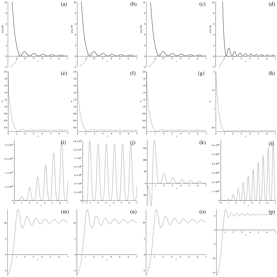
Figure 1: Behavior of Hubble parameters, size of extra dimensions, density-to-squared Hubble ratio and effective Newtonian constant with time for our model (see text for details).

As we said, we solved numerically system under consideration to see the future and past behavior. The results are presented in Fig. 1. There the first row ((a), (b), (c) and (d) panels) presents the Hubble parameters associated with $(3+1)$ (in black) and extra dimensions (in grey), the second row ((e), (f), (g) and (h) panels) shows us the size of extra dimensions $b(t)$, the third row ((i), (j), (k) and (l) panels) visualizes $G_{N,eff}H(t)^{2}/\rho(t)$ (we comment on it later) while fourth ((m), (n), (o) and (p) panels) row demonstrate effective Newtonian constant $G_{N,eff}$ from (20). All rows have four columns which correspond to four cases – first column ((a), (e), (i) and (m) panels) corresponds to $D=6$, $\omega=0.6$ case, second column ((b), (f), (j) and (n) panels) corresponds to $D=6$, $\omega=0$ case, third column ((c), (g), (k) and (o) panels) corresponds to $D=6$, $\omega=-0.6$ case while the last column ((d), (h), (l) and (p) panels) corresponds to $D=16$, $\omega=0.6$ case. This way if we compare the results between first, second and third columns, we can derive the influence of the equation of state on the dynamics while comparison of the first and fourth gives us effect of the number of extra dimensions.

Then, by comparing first three columns we can decide that the effect of the equation of state demonstrates only in the $G_{N,eff}H(t)^{2}/\rho(t)$ ratio (third row, (i), (j), (k) and (l) panels). We can see that the influence of matter on the dynamics is diminished for $\omega>0$ and significant for $\omega<0$. We comment more about it in Discussions section. In contrary the effect of the number of extra dimensions is visible for all cases – first of all, the period of oscillations is decreased for all variables (Hubble parameters, size of extra dimensions, etc) while its amplitude seems to decrease for all cases except Hubble parameters, where it increases instead.

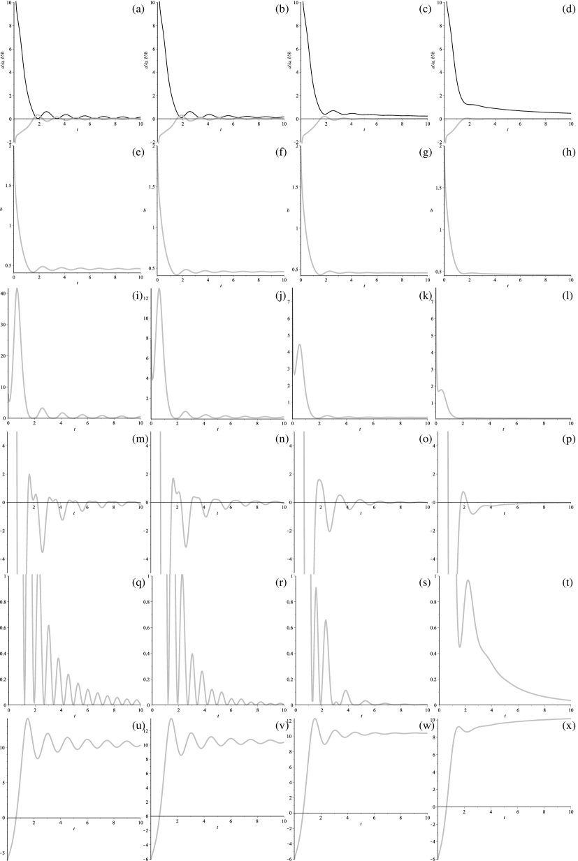
Figure 2: Similar as Fig. 1 but in the vicinity of $\omega\gtrsim-1$ (see text for details).

Also at that point it is necessary to note that $b(t)$ is reaching its predicted value (11) and the period of oscillations is in agreement with (17). This way we ensure that our model is reached indeed in our numerical study. Similar to the general compactification from geometric frustration regime CGP1 ; CGP2 , this regime is also achieved on all initial conditions which lead to the former regime with an additional (12) relation between couplings taken into account.

Regarding the influence of the equation of state, there is one more important point – for strongly negative equations of state ($\omega\lesssim-0.8$) we detected qualitative change in behavior of main variables. This change is quantitatively demonstrated in Fig. 2. In there we presented Hubble parameters (first row, (a)–(d) panels), size of extra dimensions $b(t)$ (second row, (e)–(h) panels), $H(t)^{2}/\rho(t)$ value (third row, (i)–(l) panels), Friedmann constraint (20) (fourth row, (m)–(p) panels), effective $\Lambda$-term (fifth row, (q)–(t) panels) and effective Newtonian constant (sixth row, (u)–(x) panels). These parameters are presented for four consecutive values for the equation of state: $\omega=-0.6$ (first column, (a), (e), (i), (m), (q) and (u) panels), $\omega=-0.7$ (second column, (b), (f), (j), (n), (r) and (v) panels), $\omega=-0.8$ (third column, (c), (g), (k), (o), (s) and (w) panels) and $\omega=-0.9$ (fourth column, (d), (h), (l), (p), (t) and (x) panels). One can see that the first column resemble typical behavior of Fig. 1 but with further decrease of the equation of state the behavior differ more and more. It looks like the oscillations, widely presented in Fig. 1, decaying for strongly negative equations of state in Fig. 2. If we can make mechanical analogy, the friction in Fig. 2 is so high that it prevents oscillations from occurring and we have analogue of “slow-roll” instead.

The analysis of the previous section explains oscillatory behavior, but from numerical investigation (see Figs 1 and 2) we can see that the oscillations are damped. The explanation for this lies in the fact that we perturb equations around exact solution $\dot{H}=H=0$, $\ddot{b}=\dot{b}=0$ plus (11) and (12). But in reality this asymptotic regime is achieved pretty slowly so that instead of (16) we should use full system which is very complicated for exact analytical analysis but has exponential damping, which is clearly seen from Figs. 1 and 2.

Let us note an interesting thing – formally we do not bound amplitude of described oscillations, but from Figs. 1 and 2 one can see that $H(t)$ oscillate in a way that $H(t)\geqslant 0$ always. It is easy to see why is that – if one substitute $H(t)=0$ into (4) with (12) taken into account, the resulting equation links $b(t)^{2}$ with $\dot{b}(t)^{2}$. If we further substitute this resulting relation into (6) with (12) and $H(t)=0$, we arrive to $\dot{H}=0$. This way one can see that $H(t)$ cannot cross zero and since we put $H(t)\geqslant 0$ from the beginning it always remains non-negative.

V Discussion and conclusions

In this paper we investigated the dynamical compactification in Einstein-Gauss-Bonnet gravity with arbitrary number of extra dimensions in the presence of a perfect fluid matter source. A detailed analysis was performed for the case where the theory does not admit a maximally symmetric solution. For a manifold which is a warped product of a four dimensional FRW manifold times a constant (negative) curvature compact Euclidean manifold it was found that there exists a subregime which leads to $H_{a}\to 0$ and $b(t)\to\mathop{\rm const}\nolimits$ via damped oscillations and so standard $(3+1)$-dimensional Friedmann cosmology with perfect fluid is asymptotically recovered at least at the level of the background equations.

This regime appears to be sensitive to the equation of state of the matter , and the situation here is similar to the GR limit in the $R+R^{2}$ gravity. In the latter theory there are two additional degrees of freedom connected with higher derivatives of the scale factor, so they (in contrast to Gauss-Bonnet gravity) are present in the isotropic (3+1) dimension case. They oscillate harmonically in the low-curvature limit (this is the feature of quadratic gravity, for higher order corrections the oscillation are anharmonic, see  BIT ). and can be expressed in the form of a massive scalar field. The effective equation of state for such field during oscillation is known to be $w=0$, so any matter with negative pressure would decay less rapidly, and, as a result, dominates for late time. On the contrary, a matter with a positive pressure should be subdominant in the low-curvature regime, and universe becomes dominated by gravitational degrees of freedom.

In our model the situation is quite similar. We have to additional degrees of freedom – the scale factor of “inner” dimensions and its derivative. They oscillate harmonically in the first approximation. Our numerical results show that matter content of the Universe become dominant for $w<0$ while for $w>0$ influence of the “inner” degrees of freedom may be important at later time since it decays slowly than the matter.

Another interesting numerical effect of the equation of state is the fact that for $\omega\lesssim-0.8$ an oscillatory behavior, presented in Fig. 1, is replaced with monotonic one, presented in Fig. 2. Change in the behavior could be treated with the following mechanical interpretation – the friction is increased and through this oscillations which are clearly seen in Fig. 1 are almost decayed by the last column of Fig. 2.

As for the influence of the number of extra dimensions, it manifests itself in the growing of frequency of oscillations for fixed coupling constants, which is also clear from the analytical estimation. From the technical point of view, the field equations have been written down in order to display explicitly the dependence on the number of extra dimensions. The reason is that many of the relevant physical quantities analyzed here depend on the number of extra dimensions in the same way as one would expect from a large $N$ expansion in gauge theory (in which $D$ plays the role of $N$). In particular, a clear “eikonal-like” pattern emerges. Thus, the present results strongly suggest the importance to develop a systematic $1/D$ expansion in EGB cosmology. We hope to come back on this interesting issue in a future publication.

To conclude, the aims of this paper were reached – we described new regime which is part of previously described model which allows natural and viable dynamical compactification. We demonstrated that our described regime has viable Friedmann asymptotic behavior so that at late time it cannot be distinguished from “standard” (3+1)-dimensional Friedmann model. Additionally, effective $\Lambda$-term for this model has geometrical nature which could potentially solve “cosmological constant problem” without involving any additional physics, though suffering from the fine tuning problem – the equation (12) which is exact for zero four-dimensional $\Lambda_{4D,eff}$ should be almost exactly satisfied.

- (1) T. Kaluza, Sit. Preuss. Akad. Wiss. K1, 966 (1921).
- (2) O. Klein, Z. Phys. 37, 895 (1926).
- (3) O. Klein, Nature 118, 516 (1926).
- (4) C. Garraffo and G. Giribet, Mod. Phys. Lett. A23, 1801 (2008).
- (5) D. Lovelock, J. Math. Phys. 12, 498 (1971).
- (6) R. Troncoso and J. Zanelli, Class. Quant. Grav. 17, 4451 (2000) [arXiv:hep-th/9907109].
- (7) F. Canfora, A. Giacomini, and R. Troncoso, Phys. Rev. D 77, 024002 (2008).
- (8) F. Canfora, A. Giacomini, and S. Willison, Phys. Rev. D 76, 044021 (2007).
- (9) F. Canfora and A. Giacomini, Phys. Rev. D 78, 084034 (2008).
- (10) F. Canfora and A. Giacomini, Phys. Rev. D 82, 024022 (2010).
- (11) A. Anabalon, F. Canfora, A. Giacomini, J. Oliva, Phys. Rev. D 84, 084015 (2011).
- (12) F. Canfora, A. Giacomini and S. A. Pavluchenko, Phys. Rev. D 88, 064044 (2013).
- (13) F. Canfora, A. Giacomini and S. A. Pavluchenko, Gen. Rel. Grav. 46 1805 (2014).
- (14) F. Mller-Hoissen, Phys. Lett. 163B, 106 (1985).
- (15) N. Deruelle and L. Fariña-Busto, Phys. Rev. D 41, 3696 (1990).
- (16) F. Canfora, A. Giacomini, R. Troncoso and S. Willison, Phys. Rev. D 80, 044029 (2009)
- (17) F. Mller-Hoissen, Class. Quant. Grav. 3, 665 (1986).
- (18) J. Demaret, H. Caprasse, A. Moussiaux, P. Tombal, and D. Papadopoulos, Phys. Rev. D 41, 1163 (1990).
- (19) G. A. Mena Marugán, Phys. Rev. D 46, 4340 (1992).
- (20) E. Elizalde, A.N. Makarenko, V.V. Obukhov, K.E. Osetrin, and A.E. Filippov, Phys. Lett. B644, 1 (2007).
- (21) K.I. Maeda and N. Ohta, Phys. Rev. D 71, 063520 (2005).
- (22) K.I. Maeda and N. Ohta, JHEP 1406, 095 (2014).
- (23) T. Torii and H. Maeda, Phys. Rev. D 71, 124002 (2005).
- (24) T. Torii and H. Maeda, Phys. Rev. D 72, 064007 (2005).
- (25) J. Grain, A. Barrau, and P. Kanti, Phys. Rev. D 72, 104016 (2005).
- (26) R. Cai and N. Ohta, Phys. Rev. D 74, 064001 (2006).
- (27) H. Maeda, Phys. Rev. D 73, 104004 (2006).
- (28) M. Nozawa and H. Maeda, Class. Quant. Grav. 23, 1779 (2006).
- (29) H. Maeda, Class. Quant. Grav. 23, 2155 (2006).
- (30) M. Dehghani and N. Farhangkhah, Phys. Rev. D 78, 064015 (2008).
- (31) H. Ishihara, Phys. Lett. B179, 217 (1986).
- (32) N. Deruelle, Nucl. Phys. B327, 253 (1989).
- (33) S.A. Pavluchenko and A.V. Toporensky, Mod. Phys. Lett. A24, 513 (2009).
- (34) S.A. Pavluchenko, Phys. Rev. D 80, 107501 (2009).
- (35) S.A. Pavluchenko, Phys. Rev. D 82, 104021 (2010).
- (36) V. Ivashchuk, Int. J. Geom. Meth. Mod. Phys. 7, 797 (2010) arXiv: 0910.3426.
- (37) I.V. Kirnos, A.N. Makarenko, S.A. Pavluchenko, and A.V. Toporensky, General Relativity and Gravitation 42, 2633 (2010).
- (38) S.A. Pavluchenko and A.V. Toporensky, Gravitation and Cosmology 20, 127 (2014); arXiv: 1212.1386.
- (39) I.V. Kirnos, S.A. Pavluchenko, and A.V. Toporensky, Gravitation and Cosmology 16, 274 (2010) arXiv: 1002.4488.
- (40) D. Chirkov, S. Pavluchenko, A. Toporensky, Mod. Phys. Lett. A29, 1450093 (2014); arXiv: 1401.2962.
- (41) D. Chirkov, S. Pavluchenko, A. Toporensky, Gen. Rel. Grav. 46 1799 (2014); arXiv: 1403.4625.
- (42) D. Chirkov, S. Pavluchenko, A. Toporensky, Gen. Rel. Grav. 47 137 (2015); arXiv:1501.04360.
- (43) S.A. Pavluchenko, Phys. Rev. D 92, 104017 (2015).
- (44) D. Castor and C. Senturk, Class. Quant. Grav. 32, 18 (2015).
- (45) G. ’t Hooft, Nucl. Phys. B72, 461 (1974); ibid. B75, 461 (1974).
- (46) G. Veneziano, Nucl. Phys. B117, 519 (1976).
- (47) Y. Makeenko, Large-N Gauge Theories, Lectures at the 1999 NATO-ASI on Quantum Geometry in Akureyri, Iceland [hep-th/0001047]; A. V. Manohar, Large N QCD, Les Houches Lectures (1997) [hep-ph/9802419].
- (48) F. Canfora, Nucl. Phys. B731, 389 (2005); F. Canfora, Phys. Rev. D 74, 064020 (2006).
- (49) F. Canfora, A. Giacomini and A. R. Zerwekh, Phys. Rev. D 80, 084039 (2009) [arXiv:0908.2077 [gr-qc]].
- (50) J.A. Wolf, Spaces of constant curvature, 4th edition (Publish or Perish, Wilmington, Delaware USA, 1984), p. 69.
- (51) E.E. Bukzhalev, M.M. Ivanov and A.V. Toporensky, Class. Quant. Grav. 31, 045017 (2014).