deBInfer: Bayesian inference for dynamical models of biological systems in R

Abstract

1. Understanding the mechanisms underlying biological systems, and ultimately, predicting their behaviours in a changing environment requires overcoming the gap between mathematical models and experimental or observational data. Differential equations (DEs) are commonly used to model the temporal evolution of biological systems, but statistical methods for comparing DE models to data and for parameter inference are relatively poorly developed. This is especially problematic in the context of biological systems where observations are often noisy and only a small number of time points may be available.

2. The Bayesian approach offers a coherent framework for parameter inference that can account for multiple sources of uncertainty, while making use of prior information. It offers a rigorous methodology for parameter inference, as well as modelling the link between unobservable model states and parameters, and observable quantities.

3. We present deBInfer, a package for the statistical computing environment R, implementing a Bayesian framework for parameter inference in DEs. deBInfer  provides templates for the DE model, the observation model and data likelihood, and the model parameters and their prior distributions. A Markov chain Monte Carlo (MCMC) procedure processes these inputs to estimate the posterior distributions of the parameters and any derived quantities, including the model trajectories. Further functionality is provided to facilitate MCMC diagnostics, the visualisation of the posterior distributions of model parameters and trajectories, and the use of compiled DE models for improved computational performance.

4. The templating approach makes deBInfer applicable to a wide range of DE models. We demonstrate its application to ordinary and delay DE models for population ecology.

Keywords: parameter estimation; model calibration; ordinary differential equation; delay-differential equation; Markov chain Monte Carlo; chytridiomycosis;

1 Introduction

The use of differential equations (DEs) to model dynamical systems has a long and fruitful tradition in biological disciplines such as epidemiology, population ecology, and physiology (Volterra, 1926; Kermack & McKendrick, 1927). As DE models are used in an attempt to understand biological systems, it is becoming clear that the simplest models cannot capture the rich variety of dynamics observed in them (Evans et al., 2013). However, more complex models come at the expense of additional states and/or parameters, and require more information for parameterization. Further, as most observational datasets contain uncertainty, model identification and fitting become increasingly difficult (Lonergan, 2014). Keeping complex models tractable and testable, and linking modeled quantities to data thus requires statistical methods of similar sophistication. This is particularly relevant in biology, where data series are often short or noisy, and where the scope for observational or experimental replication may be limited.

A vast array of analytical and numerical methods exists for solving DE models as well as exploring their properties and the effect of parameter values on their dynamics (Jones, 2003; Smith, 2011). In some cases, parameters may be derived from first principles or measured directly, but often some or all parameters cannot be determined by either approach, and it is necessary to estimate them from an observational dataset.

Parameter estimation methods for DE models, and their implementation as computational tools, are still less well developed than the aforementioned system dynamics tools, and are a topic of active research.

Traditional parameter inference, also known as “model calibration” or “solving inverse problems”, has, generally, been based on the maximum likelihood principle (Brewer et al., 2008; Aster et al., 2011), which assumes the existence of a true model $\mathcal{M}_{true}$ giving rise to a true dataset $\mathcal{Y}_{true}$ such that

$$\mathcal{M}_{true}(\boldsymbol{\theta})=\mathcal{Y}_{true},$$ (1)

where $\boldsymbol{\theta}$ is the parameter set for the model. The additional assumption that the observations $\mathcal{Y}$ arise from a sum of $\mathcal{Y}_{true}$ and measurement noise that is independently and normally distributed then leads to the least squares solution that is found by minimizing the Euclidian norm of the residual,

$$||\mathcal{M}(\theta)-\mathcal{Y}||_{2}.$$ (2)

This approach has been applied to both ordinary differential equations (ODEs) (e.g. Baker et al., 2005), and simple delay-differential equations (DDEs) (e.g. Horbelt et al., 2002). It allows for point estimates of the parameters, as well as the estimation of normal confidence intervals for the parameters and the correlations between them. However, these error bounds are local in nature and thus offer limited insight into the variability that is to be expected in the model outputs.

Bayesian approaches for parameter estimation in complex, nonlinear models were established early on (e.g. Tarantola & Valette, 1982; Poole & Raftery, 2000) and they are being applied with increasing frequency to a broad range of biological models (e.g. Coelho et al., 2011; Voyles et al., 2012; Johnson et al., 2013; Smith et al., 2015). Recent methodological advances have included the application of Hamiltonian Monte Carlo to ODE models, realised in the software package Stan (Carpenter et al., 2016), particle MCMC methods (Andrieu et al., 2010), approximate Bayesian computation (ABC; e.g. Liu & West, 2001; Toni et al., 2009), and so called "plug-and-play" approaches (e.g. He et al., 2009). A suite of these methods are implemented in the R package pomp (King et al., in press). While many statistical approaches, including the one presented here, treat the numerical solution of the DE model as exact, there has also been work towards quantifying the uncertainty contained in the numerical DE solutions themselves (Chkrebtii et al., 2015).

In the Bayesian approach the model, its parameters, and the data are viewed as random variables. This approach to parameter inference is attractive, as it provides a coherent framework that allows the incorporation of uncertainty in the observations and the process, and it relaxes the assumption of normal errors. It provides us not only with full probability distributions describing the parameters, but also with probability distributions for any quantity derived from them, including the model trajectories. Further, the Bayesian framework naturally lets us incorporate prior information about the parameter values. This is particularly useful when there are known biological or theoretical constraints on parameters. For example, many biological parameters, such as body size cannot take on negative values. Using informative priors can help constrain the parameter space of the estimation procedure, aiding with parameter identifiability.

We explain the rationale behind the Bayesian approach below and describe our implementation of a fitting routine based on a Markov chain Monte Carlo (MCMC) sampler coupled to a numerical DE solver. We illustrate the application of deBInfer to a simple example, the logistic differential equation, as well as a more complex model of the reproductive life history of the fungal pathogen Batrachochytrium dendrobatidis.

2 Methods

The purpose of deBInfer is to estimate the probability distribution of the parameters of a user specified DE model $\mathcal{M}$, given an empirical dataset $\mathcal{Y}$, and accounting for the uncertainty in the data. The model takes the general form

$$\mathcal{M}\equiv\frac{d\boldsymbol{x}}{dt}=\boldsymbol{f}(\boldsymbol{x}_{t},t,\boldsymbol{\theta})$$ (3)

where $\boldsymbol{x}$ is a vector of variables evolving with time; $\boldsymbol{f}$ is a functional operator that takes a time input and a vector of continuous functions $\boldsymbol{x}_{t}(\theta)$ and generates the vector $\frac{d\boldsymbol{x}}{dt}$ as output; and $\boldsymbol{\theta}$ denotes a set of parameters. Further, we define $x_{t}(\boldsymbol{\tau})=\boldsymbol{x}(t+\boldsymbol{\tau})$. When all $\tau\in\boldsymbol{\tau}=0$ the model is represented by a system of ODEs, when any $\tau<0$ the model is represented by a system of delay-differential equations (DDEs). For the purposes of inference $\boldsymbol{\tau}$ is simply a subset of the parameters $\boldsymbol{\theta}$ that are to be estimated. deBInfer implements inference for ODEs as well as DDEs with constant delays.

Using Bayes’s Theorem (Clark, 2007) we can calculate the posterior distribution of the model parameters, given the data and the prior information as

$$\Pr(\boldsymbol{\theta}|\mathcal{Y})=\frac{\Pr(\mathcal{Y}|\boldsymbol{\theta})\Pr(\boldsymbol{\theta})}{\int\Pr(\mathcal{Y}|\boldsymbol{\theta})\Pr(\boldsymbol{\theta})d\boldsymbol{\theta}}$$ (4)

where $\Pr()$ denotes a probability, $\mathcal{Y}$ denotes the data, and $\boldsymbol{\theta}$ denotes the set of model parameters. The product in the numerator is the joint distribution, which is made up of the likelihood $\Pr(\mathcal{Y}|\boldsymbol{\theta})$ or $\mathcal{L}(\mathcal{Y}|\boldsymbol{\theta})$, which gives the probability of observing $\mathcal{Y}$ given the deterministic model $\mathcal{M}(\boldsymbol{\theta})$, and the prior distribution $\Pr(\boldsymbol{\theta})$, which represents the knowledge about $\boldsymbol{\theta}$ before the data were collected. The denominator represents the marginal distribution of the data $\Pr(\mathcal{Y})=\int\Pr(\mathcal{Y}|\boldsymbol{\theta})\Pr(\boldsymbol{\theta})d\boldsymbol{\theta}$. Before the data are collected $\mathcal{Y}$ is a random variable, but after they are collected the marginal distribution becomes a fixed quantity. This means, the inferential problem reduces to

$$\Pr(\boldsymbol{\theta}|\mathcal{Y})\propto\Pr(\mathcal{Y}|\boldsymbol{\theta})\Pr(\boldsymbol{\theta}).$$ (5)

That is, finding a specific proportionality that allows the posterior $\Pr(\boldsymbol{\theta}|\mathcal{Y})$ to be a proper probability density (or mass) function that integrates to 1.

Closed form solutions for the posterior are practically impossible to obtain for complex non-linear models with more than a few parameters, but they can be approximated, e.g. by combining the MCMC algorithm with a Metropolis-Hastings sampler (Clark, 2007). This yields a sequence of likelihoods that follow a frequency distribution which approximates the posterior distribution.

The likelihood $\mathcal{L}(\mathcal{Y}|\boldsymbol{\theta})$ describes the probability of the data for a given realization of the model $\mathcal{M}(\boldsymbol{\theta})$, and we can use the fact that the data are uncertain to derive an expression like

$$\mathcal{L}(\mathcal{Y}|\boldsymbol{\theta})=\prod_{t}\mathcal{P}(\mathcal{Y}_{t},\mu=\mathcal{Y}_{t}(\theta),\sigma^{2}=\mathcal{V}_{t})$$ (6)

where $\mathcal{P}$ is a parametric probability distribution, typically with first and second moments $\mu$ and $\sigma^{2}$, $\mathcal{Y}_{t}$ is data item $t$, and $\mathcal{V}_{t}$ is the variance associated with $\mathcal{Y}_{t}$.

Often the data $\mathcal{Y}$ contain multiple data series, e.g. time-course observations of different state variables, following different probability distributions. In this case the likelihood becomes the product over all series and each data item in each series $s$

$$\mathcal{L}(\mathcal{Y}|\boldsymbol{\theta})=\prod_{s}\prod_{t}\mathcal{P}_{s}(\mathcal{Y}_{s,t},\mu_{s}=\mathcal{Y}_{s,t}(\theta),\sigma^{2}_{s}=\mathcal{V}_{s,t}).$$ (7)

3 Implementation

deBInfer provides a framework for dynamical models consisting of a deterministic DE model and a stochastic observation model. In order to perform inference using deBInfer, the user must specify R functions or data structures representing: the DE model; an observation model, and thus the data likelihood; and declare all model and observation parameters, including prior distributions for those parameters that are to be estimated. The DE model itself can also be provided as a shared object, e.g. a compiled C function. deBInfer takes these inputs and performs MCMC to sample from the posterior distributions of parameters, solving the DE model numerically within the MCMC procedure. The MCMC procedure for deBInfer offers independent, as well as random-walk Metropolis-Hastings updates and is implemented fully in R (R Core Team, 2015). Background on Metropolis-Hastings MCMC are widely available in the literature (e.g. Clark, 2007; Brooks et al., 2011).

Table 1: Implementation of the random-walk Metropolis-Hastings algorithm. The transition from a parameter value $\theta^{(k)}$ in the Markov chain at step $k$ to its value at step $k+1$ proceeds via the outlined steps. $q$ is a conditional density, the so called proposal distribution.

1. Generate a proposal $\theta^{(*)}\sim q(\theta^{(*)}|\theta^{(k)})$ 2. Evaluate the prior probability $\Pr(\theta^{(*)})$ 3. if $\Pr(\theta^{(*)})=0$ Let $\theta^{(k+1)}\leftarrow\theta^{(k)}$ 4. if $\Pr(\theta^{(*)})\neq 0$ if $\theta\in\boldsymbol{\theta}_{DE}$: solve the DE model Let $\theta^{(k+1)}\leftarrow\begin{cases}\theta^{(*)}&\hbox{{ with probability} }\ \rho(\theta^{(k)},\theta^{(*)}),\cr\theta^{(k)}&\hbox{{ with probability} }\ 1-\rho(\theta^{(k)},\theta^{(*)}),\cr\end{cases}$ where $\rho(\theta^{(k)},\theta^{(*)})=\min\left\{\dfrac{\Pr(\boldsymbol{\theta}^{(*)}|\mathcal{Y})}{\Pr(\boldsymbol{\theta}^{(k)}|\mathcal{Y})}\;\dfrac{q(\theta^{(k)}|\theta^{(*)})}{q(\theta^{(*)}|\theta^{(k)})}\;,1\right\}$

As numerically solving the DE model is the most computationally costly step, we made two slight modifications to the basic Metropolis-Hastings algorithms. (i) deBInfer makes a distinction between the parameters of the DE model $\boldsymbol{\theta}_{DE}$, and the observation parameters $\boldsymbol{\theta}_{obs}$, invoking the solver only for updates of the former, and (ii) the prior probability of each parameter proposal from the random walk sampler is evaluated before the posterior density and the acceptance ratio are calculated. This allows the rejection of proposals outside the prior support without invoking the numerical solver. The algorithm is outlined in Table 1.

deBInfer provides a choice of three proposal distributions $q$ for the first step in the algorithm, a normal $\mathcal{N}(\theta^{(k)},\sigma^{2}_{prop})$, an asymmetric uniform $\mathcal{U}(\frac{a}{b}\theta^{(k)},\frac{b}{a}\theta^{(k)})$ and a multivariate normal $\mathcal{N}(\boldsymbol{\theta}^{(k)},\boldsymbol{\Sigma})$. deBInfer requires manual tuning, i.e. the variance components $\sigma^{2}_{prop}$, $a$ and $b$, and $\boldsymbol{\Sigma}$, respectively, are user specified inputs. The asymmetric uniform distribution is useful for proposals of parameters that are strictly positive, such as variances, and the multivariate normal is useful for efficiently sampling parameters that are strongly correlated, as is often the case for DE model parameters.

4 A simple example - logistic population growth

Table 2: An overview of the main functions available in deBInfer.

Function	Description
debinfer_par	creates a data structure representing an individual parameter or initial value of the DE model, or an observation parameter, and the corresponding values, priors, etc.
setup_debinfer	combines multiple parameter declarations into an input object for inference
de_mcmc	conducts MCMC inference on a DE model and returns an object of the class debinfer_result.
plot.debinfer_result	Plots traces and posterior densities (wrapper for coda::plot.mcmc).
summary.debinfer_result	Summary statistics for MCMC samples (wrapper for coda::summary.mcmc).
pairs.debinfer_result	Pairwise plots and correlations of marginal posterior distributions.
post_prior_densplot	Overlay of posterior and prior densities for free parameters.
post_sim	Simulate posterior trajectories of the DE model and summary statistics thereof.
plot.post_sim_list	Plot posterior DE model trajectories.

We illustrate the steps needed to perform inference for a DE model, by conducting inference on the logistic model (acknowledging that the existence of a closed form solution to this DE makes this an artificial example):

$$\frac{dN}{dt}=rN\left(1-\frac{N}{K}\right).$$ (8)

Annotated code to implement this model, simulate observations from it, and conduct the inference is provided as a package vignette (Appendix A). An overview of the core functions available in deBInfer is provided in Table 2.

4.1 Installation

The deBInfer package is available on CRAN. The development version can be installed from github using devtools (Wickham & Chang, 2016), which can be installed from CRAN.

commandchars=
{},,,

\CommentTok{#Install the CRAN release.}\KeywordTok{install.packages}\NormalTok{(}\StringTok{"deBInfer"}\NormalTok{)}\CommentTok{#Alternatively install devtools and the development version of deBInfer.}\KeywordTok{install.packages}\NormalTok{(}\StringTok{"devtools"}\NormalTok{)}\NormalTok{devtools::}\KeywordTok{install_github}\NormalTok{(}\StringTok{"pboesu/debinfer"}\NormalTok{) }\CommentTok{#Load deBInfer. }\KeywordTok{library}\NormalTok{(deBInfer)}

4.2 Specification of the differential equation model

deBInfer makes use of the deSolve and PBSddesolve packages (Soetaert et al., 2010; Couture-Beil et al., 2014) to numerically solve ODE and DDE models. The DE model has to be specified as a function containing the model equations, following the guidelines given in the respective package documentations. For our simple example the function takes three inputs: time, a vector of time points at which to evaluate the DE, y, a vector containing the initial value for the state variable $N$, and parms, a vector containing the parameters $r$ and $K$. commandchars=
{},,,

\NormalTok{logistic_model <-}\StringTok{ }\NormalTok{function(time, y, parms) \{ }  \KeywordTok{with}\NormalTok{(}\KeywordTok{as.list}\NormalTok{(}\KeywordTok{c}\NormalTok{(y, parms)), \{}    \NormalTok{dN <-}\StringTok{ }\NormalTok{r *}\StringTok{ }\NormalTok{N *}\StringTok{ }\NormalTok{(}\DecValTok{1} \NormalTok{-}\StringTok{ }\NormalTok{N /}\StringTok{ }\NormalTok{K) }    \KeywordTok{list}\NormalTok{(dN)}  \NormalTok{\})}\NormalTok{\}}

4.3 Observation model and likelihood specification

For the purpose of demonstration we will conduct inference on simulated observations from this model assuming log-normal noise with a standard deviation $\sigma^{2}_{obs}$. A set of simulated observations is provided with the package and can be loaded with the command data(logistic). The appropriate log-likelihood takes the form

$$\ell(\mathcal{Y}|\boldsymbol{\theta})=\sum_{t}\ln\left(\frac{1}{\tilde{N_{t}}\sigma_{obs}\sqrt{2\pi}}\exp\left(-\frac{(\ln\tilde{N_{t}}-\ln(N_{t}+\varepsilon))^{2}}{2\sigma^{2}_{obs}}\right)\right)$$ (9)

where $\tilde{N}_{t}$ are the observations, and $N_{t}$ are the predictions of the DE model given the current MCMC sample of the parameters $\boldsymbol{\theta}$. Further, $\varepsilon\ll 1$ is a small correction needed, because the exact DE solution can equal zero (or less, depending on numerical precision of the solver). $\varepsilon$ should therefore be at least as large as the expected numerical precision of the solver. We chose $\varepsilon=10^{-6}$, which is on the same order as the default numerical precision of the default solver (deSolve::ode with method = "lsoda"), but we found that the inference results were insensitive to this choice as long as $\varepsilon\leq 0.01$ (Appendix A, Section 7).

The deBInfer observation model template requires three inputs: a data.frame of observations, data; the simulated trajectory returned by the numerical solver in MCMC procedure, sim.data; and the current sample of the parameters, samp. The user specifies the observation model such that it returns the summed log-likelihoods of the data. In this example the observations are in the data.frame column N_noisy, and the corresponding predicted states are in the column N of the matrix-like object sim.data (see Appendix A). commandchars=
{},,,

\CommentTok{#load example data}\KeywordTok{data}\NormalTok{(logistic)}\CommentTok{# user defined data likelihood}\NormalTok{logistic_obs_model <-}\StringTok{ }\NormalTok{function(data, sim.data, samp)\{}  \NormalTok{epsilon <-}\StringTok{ }\FloatTok{1e-6}  \NormalTok{llik <- }\KeywordTok{sum}\NormalTok{(}\KeywordTok{dlnorm}\NormalTok{(data$N_noisy, }\DataTypeTok{meanlog = }\KeywordTok{log}\NormalTok{(sim.data[, }\StringTok{"N"}\NormalTok{]+ epsilon),}                     \DataTypeTok{sdlog = }\NormalTok{samp[[}\StringTok{"sdlog.N"}\NormalTok{]],}\DataTypeTok{log = }\OtherTok{TRUE}\NormalTok{))}  \KeywordTok{return}\NormalTok{(llik) }  \NormalTok{\}}

4.4 Parameter, prior, and sampler specification

All parameters that are used in the DE model and the observation model need to be declared for the inference procedure using the debinfer_par() function. The declaration describes the variable name, whether it is a DE or observation parameter and whether or not it is to be estimated. If the parameter is to be estimated, the user also needs to specify a prior distribution and a number of additional parameters for the MCMC procedure. debinfer currently supports priors from all probability distributions implemented in base R, as well as their truncated variants, as implemented in the truncdist package (Novomestky & Nadarajah, 2012).

We declare the DE model parameter $r$, assign a prior $r\sim\mathcal{N}(0,1)$ and a random walk sampler with a Normal kernel (samp.type="rw") and proposal variance of 0.005 with the command commandchars=
{},,,

\NormalTok{r <-}\StringTok{ }\KeywordTok{debinfer_par}\NormalTok{(}\DataTypeTok{name =} \StringTok{"r"}\NormalTok{, }\DataTypeTok{var.type =} \StringTok{"de"}\NormalTok{, }\DataTypeTok{fixed =} \OtherTok{FALSE}\NormalTok{,}                \DataTypeTok{value =} \FloatTok{0.5}\NormalTok{, }\DataTypeTok{prior = }\StringTok{"norm"}\NormalTok{, }\DataTypeTok{hypers = }\KeywordTok{list}\NormalTok{(}\DataTypeTok{mean =} \DecValTok{0}\NormalTok{, }\DataTypeTok{sd =} \DecValTok{1}\NormalTok{),}                \DataTypeTok{prop.var = }\FloatTok{0.005}\NormalTok{, }\DataTypeTok{samp.type = }\StringTok{"rw"}\NormalTok{)}Similarly, we declare $K\sim\ln\mathcal{N}(1,1)$ and $\sigma^{2}_{obs}\sim\ln\mathcal{N}(0,1)$. commandchars=
{},,,

\NormalTok{K <-}\StringTok{ }\KeywordTok{debinfer_par}\NormalTok{(}\DataTypeTok{name =} \StringTok{"K"}\NormalTok{, }\DataTypeTok{var.type =} \StringTok{"de"}\NormalTok{, }\DataTypeTok{fixed =} \OtherTok{FALSE}\NormalTok{,}                \DataTypeTok{value =} \DecValTok{5}\NormalTok{, }\DataTypeTok{prior = }\StringTok{"lnorm"}\NormalTok{, }\DataTypeTok{hypers = }\KeywordTok{list}\NormalTok{(}\DataTypeTok{meanlog =} \DecValTok{1}\NormalTok{, }\DataTypeTok{sdlog =} \DecValTok{1}\NormalTok{),}                \DataTypeTok{prop.var = }\FloatTok{0.1}\NormalTok{, }\DataTypeTok{samp.type = }\StringTok{"rw"}\NormalTok{)}\NormalTok{sdlog.N <-}\StringTok{ }\KeywordTok{debinfer_par}\NormalTok{(}\DataTypeTok{name =} \StringTok{"sdlog.N"}\NormalTok{, }\DataTypeTok{var.type =} \StringTok{"obs"}\NormalTok{, }\DataTypeTok{fixed =} \OtherTok{FALSE}\NormalTok{,}                \DataTypeTok{value =} \FloatTok{0.1}\NormalTok{, }\DataTypeTok{prior = }\StringTok{"lnorm"}\NormalTok{, }\DataTypeTok{hypers = }\KeywordTok{list}\NormalTok{(}\DataTypeTok{meanlog =} \DecValTok{0}\NormalTok{, }\DataTypeTok{sdlog =} \DecValTok{1}\NormalTok{),}                \DataTypeTok{prop.var = }\KeywordTok{c}\NormalTok{(}\DecValTok{3}\NormalTok{,}\DecValTok{4}\NormalTok{), }\DataTypeTok{samp.type = }\StringTok{"rw-unif"}\NormalTok{)}Note that we are using the asymmetric uniform proposal distribution for the variance parameter (samp.type="rw-unif"), as this ensures strictly positive proposals. Lastly, we provide an initial value $N_{0}=0.1$ for the DE: commandchars=
{},,,

\NormalTok{N <-}\StringTok{ }\KeywordTok{debinfer_par}\NormalTok{(}\DataTypeTok{name =} \StringTok{"N"}\NormalTok{, }\DataTypeTok{var.type =} \StringTok{"init"}\NormalTok{, }\DataTypeTok{fixed =} \OtherTok{TRUE}\NormalTok{, }\DataTypeTok{value =} \FloatTok{0.1}\NormalTok{)}

4.5 MCMC inference

The MCMC procedure is called using the function de_mcmc() which takes the declared parameters, the DE and observational models, the data, and further optional arguments to the MCMC procedure and/or the solver as inputs and returns an array containing the resulting MCMC samples.

All declared parameters are collated using setup_debinfer()

commandchars=
{},,,

\NormalTok{mcmc.pars <-}\StringTok{ }\KeywordTok{setup_debinfer}\NormalTok{(r, K, sdlog.N, N)}and passed to de_mcmc() which is set to use deSolve::ode() as a backend in this case, as specified by the argument solver = "ode" commandchars=
{},,,

\CommentTok{# do inference with deBInfer}\CommentTok{# MCMC iterations}\NormalTok{iter <-}\StringTok{ }\DecValTok{5000}\CommentTok{# inference call}\NormalTok{mcmc_samples <-}\StringTok{ }\KeywordTok{de_mcmc}\NormalTok{(}\DataTypeTok{N =} \NormalTok{iter, }\DataTypeTok{data = }\NormalTok{logistic, }\DataTypeTok{de.model = }\NormalTok{logistic_model, }                          \DataTypeTok{obs.model = }\NormalTok{logistic_obs_model, }\DataTypeTok{all.params = }\NormalTok{mcmc.pars,}                          \DataTypeTok{Tmax =} \KeywordTok{max}\NormalTok{(logistic$time), }\DataTypeTok{data.times = }\NormalTok{logistic$time, }                          \DataTypeTok{cnt = }\DecValTok{500}\NormalTok{, }\DataTypeTok{plot = }\OtherTok{FALSE}\NormalTok{, }\DataTypeTok{solver = }\StringTok{"ode"}\NormalTok{)}

4.6 Inference Outputs

The inference function returns an object of class debinfer_result, which contains the posterior samples in a format compatible with the coda package (Plummer et al., 2006), as well as the DE and observation models and all parameters used for inference. This allows the use of the diagnostic functions and plotting routines provided in coda (see Fig. 1). We also provide additional functions and methods such as pairs.debinfer_result() to create pairwise plots of the marginal posterior distributions, which show correlations between individual parameters (see Fig. 2), post_prior_densplot(), which allows a visual comparison between prior and marginal posterior densities for each parameter, post_sim() which simulates posterior model trajectories and associated credible intervals, as well as plotting methods for the latter (see Fig. 3).

Figure 1: MCMC traces and posterior density plots for the logistic model. Figures like this one can be created using plot.debinfer_result.

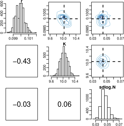
Figure 2: Pairwise plot of the marginal posterior distributions. This figure was created using pairs.debinfer_result.

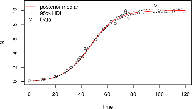
Figure 3: Posterior model trajectory (median with 95% highest posterior density interval), created with plot.post_sim_list, and the data points used for fitting.

5 Example application - DDE model of fungal population growth

To illustrate applications of deBInfer beyond the simplistic example above, we outline inference procedures for a more complex model and corresponding observational data. Full model details and annotated code can be found in Appendix B.

Our example demonstrates parameter inference for a DDE model of population growth in the environmentally sensitive fungal pathogen Batrachochytrium dendrobatidis (Bd), which causes the amphibian disease chytridiomycosis (Rosenblum et al., 2010; Voyles et al., 2012). This model has been used to further our understanding of pathogen responses to changing environmental conditions. Further details about the model development, and the experimental procedures yielding the data used for parameter inference can be found in Voyles et al. (2012).

The model follows the dynamics of the concentration of an initial cohort of zoospores, $C$, the concentration of zoospore-producing sporangia, $S$, and the concentration of zoospores in the next generation $Z$. The initial cohort of zoospores, $C$, starts at a known concentration, and zoospores in this initial cohort settle and become sporangia at rate $s_{r}$, or die at rate $\mu_{Z}$. $f_{s}$ is the fraction of sporangia that survive to the zoospore-producing stage. We assume that it takes a minimum of $T_{min}$ days before the sporangia produce zoospores, after which they produce zoospores at rate $\eta$. Zoospore-producing sporangia die at rate $d_{s}$. The concentration of zoospores, $Z$, is the only state variable measured in the experiments, and it is assumed that these zoospores settle ($s_{r}$) or die ($\mu_{Z}$) at the same rates as the initial cohort of zoospores. The equations that describe the population dynamics are as follows:

$$\frac{dC}{dt} =-(s_{r}+\mu_{Z})C(t)$$ (10)

$$\frac{dS}{dt} =s_{r}f_{s}C(t-T_{min})-d_{s}S(t)$$ (11)

$$\frac{dZ}{dt} =\eta S(t)-(s_{r}+\mu_{Z})Z(t)$$ (12)

Because the observations are counts of zoospores (i.e. discrete numbers), we assume that observations of the system at a set of discrete times $t^{\prime}$ are independent Poisson random variables with a mean given by the solution of the DDE, at times $t^{\prime}$.

The log-likelihood of the data given the parameters, underlying model, and initial conditions is then a sum over the $n$ observations at each time point in $t^{\prime}$

$$\ell(\mathbf{Z}|\mathbf{\theta})=\sum\limits^{n}_{t}Z_{t}\text{ log }\lambda-n\lambda$$ (13)

In this case we conduct inference using deSolve::dede() as the backend to de_mcmc. The marginal posteriors of the estimated parameters are presented in Fig. 4, and posterior trajectories for the model are presented in Fig. 5.

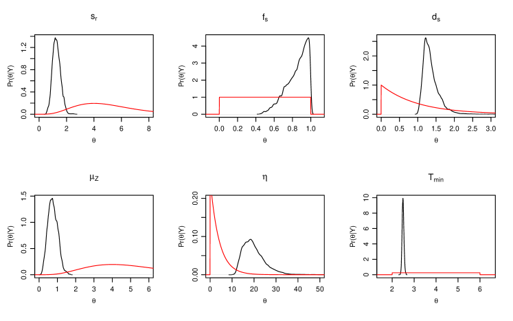
Figure 4: Comparison of marginal posterior densities (black) and the corresponding priors (red) of the estimated parameters of the chytrid model. This plot was created using post_prior_densplot.

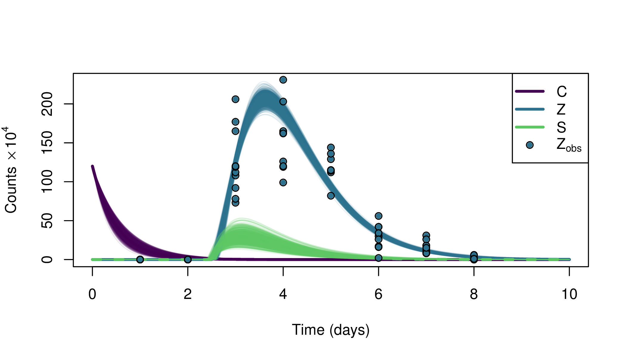
Figure 5: Posterior trajectories for each state variable of the chytrid model based on 1000 model simulations from the posterior of the parameters and the data points $Z_{obs}$ used for fitting.

6 Known limitations

The MCMC sampler is implemented in R, which makes it considerably slower than samplers written in compiled languages e.g., those underlying packages such as Stan (Carpenter et al., 2016) or Filzbach (Purves & Lyutsarev, 2016). For inference conducted purely in R, the computational bottleneck is solving the DE model numerically. However, even for relatively simple models, a 5-10 fold speed up of the inference procedure can be achieved by using compiled DE models (see Appendix C) . Furthermore, the debinfer MCMC algorithm is not adaptive and requires manual tuning. Lastly, sampling using the Metropolis-Hastings MCMC algorithm itself can be inefficient in the presence of strong parameter correlations. Alternative approaches such as Hamiltonian MC (Carpenter et al., 2016) or particle-filtering methods (e.g. King et al., in press) may offer more efficient means for parameter estimation in ODEs in these cases. Nonetheless, the package is able to fit real world problems in a matter of minutes to hours on current desktop hardware, which is acceptable for many applications, while providing flexible inference for both ODE and DDE models.

7 Conclusion

Understanding the mechanisms underlying biological systems, and ultimately, predicting their behaviours in a changing environment requires overcoming the gap between mathematical models and experimental or observational data. We believe that Bayesian inference provides a powerful tool for fitting dynamical models and selecting between competing models. The deBInfer R package provides a suite of tools to this end in a programming language that is widespread in many biological disciplines. We hope that our package, will lower the hurdle to the uptake of this inference approach for empirical biologists. We encourage users to report bugs and provide other feedback on the project issue page: https://github.com/pboesu/debinfer/issues

8 Acknowledgements

We thank Richard FitzJohn and two anonymous reviewers for their constructive comments on earlier versions of the code and manuscript. All authors were supported by the U.S. National Science Foundation (Grant PLR-1341649). We thank Jamie Voyles for sharing the chytrid growth data. The authors have no conflict of interest to declare.

9 Data Accessibility

All code and data used in this article are included in the deBInfer package and its vignettes, which are freely available from CRAN: https://cran.r-project.org/package=deBInfer. The development version of the package is available at https://github.com/pboesu/debinfer.

10 Author contributions

LRJ conceived the methodology and wrote the initial R implementation; PHBS reimplemented the methodology as an R package; PHBS and SJR wrote the package documentation; PHBS led the writing of the manuscript. All authors tested the software, contributed critically to the drafts, and gave final approval for publication.

Appendix A Annotated code for the logistic DE example

This appendix can be found in the supplementary materials. It can also be displayed after installing deBInfer with the R command:
vignette("logistic_ode_example", package="deBInfer")

Appendix B Annotated code for the DDE example

This appendix can be found in the supplementary materials. It can also be displayed after installing deBInfer with the R command:
vignette("chytrid_dede_example", package="deBInfer")

Appendix C Inference for a compiled DE model

This appendix can be found in the supplementary materials. It can also be displayed after installing deBInfer with the R command:
vignette("deBInfer_compiled_code", package="deBInfer")

References

- Andrieu et al. (2010) Andrieu, C., Doucet, A. & Holenstein, R. (2010) Particle markov chain monte carlo methods. Journal of the Royal Statistical Society: Series B (Statistical Methodology), 72, 269–342.
- Aster et al. (2011) Aster, R.C., Borchers, B. & Thurber, C.H. (2011) Parameter Estimation and Inverse Problems. Academic Press, Amsterdam, 2nd edition.
- Baker et al. (2005) Baker, C.T., Bocharov, G., Ford, J.M., Lumb, P.M., Norton, S.J., Paul, C., Junt, T., Krebs, P. & Ludewig, B. (2005) Computational approaches to parameter estimation and model selection in immunology. Journal of Ccomputational and Applied mathematics, 184, 50–76.
- Boersch-Supan & Johnson (2016) Boersch-Supan, P. & Johnson, L. (2016) deBinfer: Bayesian inference for dynamical models of biological systems. arXiv, 1605.00021.
- Brewer et al. (2008) Brewer, D., Barenco, M., Callard, R., Hubank, M. & Stark, J. (2008) Fitting ordinary differential equations to short time course data. Philosophical Transactions of the Royal Society of London A: Mathematical, Physical and Engineering Sciences, 366, 519–544.
- Brooks et al. (2011) Brooks, S., Gelman, A., Jones, G. & Meng, X.L. (2011) Handbook of Markov Chain Monte Carlo. CRC Press, Boca Raton, FL.
- Carpenter et al. (2016) Carpenter, B., Gelman, A., Hoffman, M., Lee, D., Goodrich, B., Betancourt, M., Brubaker, M.A., Guo, J., Li, P. & Riddell, A. (2016) Stan: A probabilistic programming language. Journal of Statistical Software, in press.
- Chkrebtii et al. (2015) Chkrebtii, O.A., Campbell, D.A., Calderhead, B. & Girolami, M.A. (2015) Bayesian solution uncertainty quantification for differential equations. arXiv preprint arXiv:13062365.
- Clark (2007) Clark, J.S. (2007) Models for Ecological Data: An Introduction. Princeton University Press, Princeton, New Jersey, USA.
- Coelho et al. (2011) Coelho, F.C., Codeço, C.T. & Gomes, M.G.M. (2011) A Bayesian framework for parameter estimation in dynamical models. PloS one, 6, e19616.
- Couture-Beil et al. (2014) Couture-Beil, A., Schnute, J.T., Haigh, R., Boers, N., Wood, S.N. & Cairns, B.J. (2014) PBSddesolve: Solver for Delay Differential Equations. R package version 1.11.29, http://CRAN.R-project.org/package=PBSddesolve.
- Evans et al. (2013) Evans, M.R., Grimm, V., Johst, K., Knuuttila, T., de Langhe, R., Lessells, C.M., Merz, M., O’Malley, M.A., Orzack, S.H., Weisberg, M., Wilkinson, D., Wolkenhauer, O. & Benton, T. (2013) Do simple models lead to generality in ecology? Trends in Ecology & Evolution, 28, 578–583.
- He et al. (2009) He, D., Ionides, E.L. & King, A.A. (2009) Plug-and-play inference for disease dynamics: measles in large and small populations as a case study. Journal of the Royal Society Interface.
- Horbelt et al. (2002) Horbelt, W., Timmer, J. & Voss, H. (2002) Parameter estimation in nonlinear delayed feedback systems from noisy data. Physics Letters A, 299, 513–521.
- Johnson et al. (2013) Johnson, L.R., Pecquerie, L. & Nisbet, R.M. (2013) Bayesian inference for bioenergetic models. Ecology, 94, 882–894.
- Jones (2003) Jones, D.S. (2003) Differential Equations and Mathematical Biology. Chapman & Hall, Boca Raton, FL.
- Kermack & McKendrick (1927) Kermack, W.O. & McKendrick, A.G. (1927) A contribution to the mathematical theory of epidemics. Proceedings of the Royal Society of London A: Mathematical, Physical and Engineering Sciences, 115, 700–721.
- King et al. (in press) King, A., Ionides, E., Bretó, C., Ellner, S., Kendall, B., Wearing, H., Ferrari, M., Lavine, M. & Reuman, D. (in press) pomp: Statistical inference for partially observed markov processes (r package). Journal of Statistical Software.
- Liu & West (2001) Liu, J. & West, M. (2001) Combined parameter and state estimation in simulation-based filtering. Sequential Monte Carlo methods in practice, pp. 197–223. Springer.
- Lonergan (2014) Lonergan, M. (2014) Data availability constrains model complexity, generality, and utility: a response to evans et al. Trends in Ecology & Evolution, 29, 301–302.
- Novomestky & Nadarajah (2012) Novomestky, F. & Nadarajah, S. (2012) truncdist: Truncated Random Variables. R package version 1.0-1, http://CRAN.R-project.org/package=truncdist.
- Plummer et al. (2006) Plummer, M., Best, N., Cowles, K. & Vines, K. (2006) Coda: Convergence diagnosis and output analysis for MCMC. R News, 6, 7–11.
- Poole & Raftery (2000) Poole, D. & Raftery, A.E. (2000) Inference for deterministic simulation models: the Bayesian melding approach. Journal of the American Statistical Association, 95, 1244–1255.
- Purves & Lyutsarev (2016) Purves, D. & Lyutsarev, V. (2016) Fit complex models to hetereogenous data: Bayesian and likelihood analysis made easy. Http://research.microsoft.com/en-us/um/cambridge/groups/science/tools/filzbach/filzbach.htm [accessed 06 September 2016].
- R Core Team (2015) R Core Team (2015) R: A Language and Environment for Statistical Computing. R Foundation for Statistical Computing, Vienna, Austria. Http://www.R-project.org/.
- Rosenblum et al. (2010) Rosenblum, E.B., Voyles, J., Poorten, T.J. & Stajich, J.E. (2010) The deadly chytrid fungus: A story of an emerging pathogen. PLoS Pathogens, 6, 1–3.
- Smith (2011) Smith, H. (2011) An Introduction to Delay Differential Equations with Applications to the Life Sciences. Springer Verlag, New York, NY.
- Smith et al. (2015) Smith, M.J., Tittensor, D.P., Lyutsarev, V. & Murphy, E. (2015) Inferred support for disturbance-recovery hypothesis of North Atlantic phytoplankton blooms. Journal of Geophysical Research: Oceans, 120, 7067–7090.
- Soetaert et al. (2010) Soetaert, K., Petzoldt, T. & Setzer, R.W. (2010) Solving differential equations in R: package deSolve. Journal of Statistical Software, 33, 1–25.
- Tarantola & Valette (1982) Tarantola, A. & Valette, B. (1982) Inverse problems = quest for information. Journal of Geophysics, 50, 150–170.
- Toni et al. (2009) Toni, T., Welch, D., Strelkowa, N., Ipsen, A. & Stumpf, M.P. (2009) Approximate bayesian computation scheme for parameter inference and model selection in dynamical systems. Journal of the Royal Society Interface, 6, 187–202.
- Volterra (1926) Volterra, V. (1926) Fluctuations in the abundance of a species considered mathematically. Nature, 118, 558–560.
- Voyles et al. (2012) Voyles, J., Johnson, L.R., Briggs, C.J., Cashins, S.D., Alford, R.A., Berger, L., Skerratt, L.F., Speare, R. & Rosenblum, E.B. (2012) Temperature alters reproductive life history patterns in Batrachochytrium dendrobatidis, a lethal pathogen associated with the global loss of amphibians. Ecology and Evolution, 2, 2241–2249.
- Wickham & Chang (2016) Wickham, H. & Chang, W. (2016) devtools: Tools to Make Developing R Packages Easier. R package version 1.10.0, http://CRAN.R-project.org/package=devtools.