Nonparametric $M$-estimation for right censored regression model with stationary ergodic data

Abstract

The present paper deals with a nonparametric $M$-estimation for right censored regression model with stationary ergodic data. Defined as an implicit function, a kernel type estimator of a family of robust regression is considered when the covariate take its values in $\mathbb{R}^{d}$ ($d\geq 1$) and the data are sampled from stationary ergodic process. The strong consistency (with rate) and the asymptotic distribution of the estimator are established under mild assumptions. Moreover, a usable confidence interval is provided which does not depend on any unknown quantity. Our results hold without any mixing condition and do not require the existence of marginal densities. A comparison study based on simulated data is also provided.

Keywords: Asymptotic normality, censored data, confidence interval, ergodic data, Kaplan-Meier estimator, robust estimation, strong consistency, synthetic data.

Subject Classifications: 60F10, 62G07, 62F05, 62H15.

1 Introduction

Consider a pair $(X,T)$ of random variables defined in $\mathbb{R}^{d}\times\mathbb{R}$, $d\geq 1$, where $T$ is a variable of interest and $X=(X^{1},\dots,X^{d})$ a vector of concomitant variables. In many situations, one can be interested in the regression function $m(x)=\mathbb{E}(T|X=x)$ for $x\in\mathbb{R}^{d}$, which allows to describe the relationship between T and X.

Let $\rho(\cdot)$ be a continuous differentiable function such that $\partial\rho(\cdot)/\partial\theta=:\psi(\cdot)$ is supposed to be nondecreasing real-valued function. Let us denote by $m_{\psi}(\cdot)$ the location parameter (or equivalently the $\psi$-regression function) that defined as a solution, with respect to $\theta$, of the following minimization problem

$$\min_{\theta}\mathbb{E}\left[\rho(T-\theta)|X=x\right].$$ (1.1)

We call such a $m_{\psi}(\cdot)$ the $M$-functional corresponding to $\psi(\cdot)$. Notice that whenever $\rho(\cdot)$ is a regular function, $m_{\psi}(\cdot)$ may be considered as a solution, with respect to, $\theta$ of the equation

$$\mathbb{E}\left[\psi(T-\theta)\left|\right.X=x\right]=0.$$ (1.2)

We point out that the family of the robust functions $\psi(\cdot)$ may depend on $x$. This may occur when dealing with nonlinear regression models with ARCH-errors, in such case the function $\psi(\cdot)$ depends in the function $\sigma(x)$, which measures the spread of the conditional law of $T$ given $X=x$.

Let $(X_{i},T_{i})_{i=1,\dots,n}$ be $n$ copies of the pair $(X,T)$. A kernel type estimator, say $\widehat{m}_{\psi}(x)$, of $m_{\psi}(x)$ is a solution of the equation

$$\sum_{i=1}^{n}w_{n,i}(x)\psi(T_{i}-\theta)=0,$$ (1.3)

where $w_{n,i}(x):=K(h_{n}^{-1}(X_{i}-x))/\sum_{i=1}^{n}K(h_{n}^{-1}(X_{i}-x))$ are the Nadaraya-Watson (NW) weights. Here, $K(\cdot)$ is a real-valued kernel function and $h:=h_{n}$ is a sequence of positive real numbers that decreases to zero as $n$ tends to infinity.

If we consider $\rho(u)=u^{2}$ (and thus $\psi(u)=u$), then $m_{\psi}(x)$ coincides with the classical regression function $m(x)$ and $\widehat{m}_{n,\psi}(x)$ is its NW estimator. When $\rho(u)=|u|$ (and therefore $\psi(u)=\mbox{sign}(u)$), then $\widehat{m}_{n,\psi}(x)$ corresponds to the local least absolute distance estimator. For more possible choices of the function $\psi(\cdot)$ the reader is referred to Serfling (1980), page 246.

In the statistical literature, several papers have been devoted to the study the properties of the nonparametric $M$-estimator defined as a solution of equation (1.3) when the variable of interest $T$ is completely observed. One can refer, among others, to Huber (1964) and Härdle (1984) for independent and identically distributed (i.i.d.) case, Collomb and Härdle (1986) and Boente and Fraiman (1989) for mixing processes and Laïb and Ould Saïd (2000) for stationary ergodic processes. Azzedine et al. (2008) established the almost complete convergence rate of the kernel type estimator in the i.i.d. case while Cai and Roussas (1992) studied its asymptotic properties under $\alpha$-mixing assumption. Crambes et al. (2008) studied the same problem for functional covariate. They established explicit exact asymptotic expression of the convergence rate in $\mathbb{L}^{p}$ norm. While Gueriballah et al. (2013) established the almost complete convergence with rate in the setting of functional and stationary ergodic data. However, in many practical situation such as in medical follow-up or in engineering life-test study, the variable of interest $T$ may not be completely observable. This case may be occur when dealing with censored data. For example, in the clinical trials domain, it frequently happens that patients from the same hospital have correlated survival times due to unmeasured variables such as the quality of hospital equipment. For further real practical examples, the reader can be referred (among others) to Wei et al. (1989) for the regression method with applied data, and Lipsitz and Ibrahim (2000) for the case of missing covariates.

The regression model in presence of censored data has been studied by several authors. For instance Cox (1972) considered the linear regression model and estimated the slope via the proportional hazard model. In the general linear case, many approaches have been used, see for instance Koul et al. (1981) and Koul and Stute (1998) . Ren and Gu (1997) proposed a type $M$-estimators for the linear regression model with random design when the response observations are doubly censored. For nonlinear regression model, Beran (1981) introduced a class of nonparametric estimators for the conditional survival function in the presence of right-censoring. He proved some consistency results of these estimates, his work has extended by Dabrowska, D.M. (1987, 1989). Jin (2007) constructed an $M$-estimators for the regression parameters in semi parametric linear models for censored data and established asymptotic normality of these estimators.

Notice that, the estimator of the conditional survival function could be used in order to get a consistent estimate of the regression function $m(\cdot)$ in the presence of censored data. However, the computations may be difficult practically. To overcome this drawback, Carbonez el al. (1995) introduced a general nonparametric partitioning estimate of $m(\cdot)$ and proved its strong consistency. Kohler et al. (2002) gave a simpler proof for kernel, nearest neighbor, least squares and penalized least squares estimates.

In all papers mentioned above when dealing with dependent data the condition of $\alpha$-mixing is assumed to be fulfilled. A large class of processes satisfy this condition. However, there are still a great number of models where such assumption does not hold (see Laïb and Louani (2010) for some examples). It is then necessary to consider a general larger dependency framework as is the ergodicity.

For the sake of clarity, introduce some details defining the ergodic property of processes and its link with mixing one. Let $\{X_{n},n\in\mathbb{Z}\}$ be a stationary sequence. Consider the backward field ${\cal B}_{n}=\sigma(X_{k};k\leq n)$ and the forward field ${\cal F}_{m}=\sigma(X_{k};k\geq m)$. The sequence is strongly mixing if

$$\sup_{A\in{\cal B}_{0},B\in{\cal B}_{n}}|\mathbb{P}(A\cap B)-\mathbb{P}(A)\mathbb{P}(B)|=\varphi(n)\to 0\quad\mbox{as}\quad n\to\infty.$$

The sequence is ergodic if

$$\lim_{n\to\infty}\frac{1}{n}\sum_{k=0}^{n-1}|\mathbb{P}(A\cap\tau^{-k}B)-\mathbb{P}(A)\mathbb{P}(B)|=0,$$ (1.4)

where $\tau$ is the time-evolution or shift transformation. The naming of strong mixing in the above definition is a more stringent condition than that what ordinarily referred (when using the vocabulary of measure-preserving dynamical systems) to as strong mixing, namely that $\lim_{n\to\infty}\mathbb{P}(A\cap\tau^{-n}B)=\mathbb{P}(A)\mathbb{P}(B)$ for any two measurable sets $A,B$ (see Rosenblatt (1972)). Hence, strong mixing implies ergodicity. However, the converse is not true: there exist ergodic sequences which are not strong mixing. The ergodicity condition is then a naturel condition and lower than any type of mixing for which usual nonparametric estimators (density, regression, …) are convergent. It seems to be a condition of obtaining large numbers of law, since it is well known from the ergodic theorem that, for a stationary ergodic process $Z$, we have

$$\lim_{n\to\infty}\frac{1}{n}\sum_{i=1}^{n}Z_{i}=\mathbb{E}(Z_{1}),\ \mbox{almost surely (a.s.)}$$ (1.5)

The ergodic property in our setting is formulated on the basis of the statement (1.5) and the requirements are considered in conditions (A2) below. We refer to the book of Krengel (1985) for an account of details and results on the ergodic theory.

Recently, and in the case of complete data, Laïb and Louani (2011) studied the asymptotic properties of the regression function using functional stationary ergodic data. In the case of right censored response, Chaouch and Khardani (2013) considered the conditional quantile estimation based on functional stationary ergodic data.

In this paper, we are interested in the kernel smoothing estimation of the $\psi$-regression function for right-censored and stationary ergodic data. For more motivation concerning this kind of dependency one may refer to Laïb and Louani (2011). We emphasis that, our results hold without assuming any type of mixing conditions as well as the existence of marginal and conditional densities. This is of particular interest for chaotic models where the underlying process does not posses a marginal density (see Lu (1999) and Laïb (2005) for a discussion). To the best of our knowledge this question, under the general hypotheses cited above, has not been studied in literature. The proof our results used only technical of martingale differences combined with the ergodic property given in (1.5). We avoid to suppose any additional condition on the structure of the process under study as in the $\alpha$-mixing case.

The paper is organized as follows. In Section 2, a kernel type estimator of the $\psi$-regression is introduced for right censorship model under an ergodic assumption. Section 3 presents the assumptions under which the almost sure consistency (with rate) and the asymptotic distribution of the estimator are established. A simulation study that shows the performance of our estimator is provided in Section 4. Proofs of main results and some auxiliary results (with their proofs) are postponed in Section 5.

2 Robust regression estimation with censored data

Let us consider a triple $(X,C,T)$ of random variables defined in $\mathbb{R}^{d}\times\mathbb{R}\times\mathbb{R}$, where $T$ is the variable of interest (typically a lifetime variable), $C$ a censoring variable and $X=(X^{1},\dots,X^{d})$ a vector of covariates. We denote by $F(\cdot)$ (resp. $G(\cdot)$) the distribution function of $T$ (resp. $C$) which are supposed to be unknown and continuous. The continuity of $G$ allows to use convergence results for the Kaplan and Meier (1958) estimator of $G$. From now on, we assume that

• $(T,X)$ and $C$ are independent.

This assumption plays an important role to derive the result given by (2.2) below. It has been introduced by Carbonez el al. (1995) and used (among others) by Kohler et al. (2002) and Guessoum and Ould Saïd (2008). It is plausible whenever the censoring is independent of the characteristics of the patients under study.

In the right censorship model, the pair $(T,C)$ is not directly observed and the corresponding available information is given by $Y=\min(T,C)$ and $\delta=1\kern-1.99997pt{\rm l}_{\{T\leq C\}}$, where $1\kern-1.99997pt{\rm l}_{A}$ denotes the indicator function of the set $A$. Therefore, we assume that a sample $\{(X_{i},\delta_{i},Y_{i}),i=1,\dots,n\}$ is at our disposal. Moreover, we suppose throughout the paper that $(X_{i},T_{i})_{i=1,\dots,n}$ is a strictly stationary ergodic sequence, in the sense that satisfies the statement (1.5), and $(C_{i})_{i}$ is a sequence of (i.i.d.) r.v’s which is independent of $(X_{i},T_{i})_{i=1,\dots,n}$. One may observe that, by continuity of the identity application, the unobserved sample $(X_{i},T_{i},C_{i})_{i=1,\dots,n}$ is ergodic. In addition let $\wp:\mathbb{R}^{3}\rightarrow\mathbb{R}\times\{0,1\}\times\mathbb{R}$ be a measurable application defined by $(T,C,X)\mapsto(Y,\delta,X).$ Clearly, by the multidimensional ergodic theorem, the observed sample is stationary and ergodic one, as soon as the unobserved sample is.

When dealing with censored data, many authors (see e.g. Carbonez el al. (1995), Kohler et al. (2002) Guessoum and Ould Saïd (2012) and Lemdani and Ould Saïd (2013) among others) use the so-called synthetic data which allow to take into account the censoring effect on the lifetime distribution. To make clear this notion, let

$$Z=\frac{\delta Y}{\overline{G}(Y)},\quad\mbox{where}\quad\overline{G}(\cdot)=1-G(\cdot).$$ (2.1)

Making use of double conditioning withe respect to $(X,T)$ combined with (A0), one may write

$$\mathbb{E}\left\{Z|X\right\}=\mathbb{E}\left\{\frac{T}{\overline{G}(T)}\mathbb{E}\left(1\kern-1.99997pt{\rm l}_{\{T\leq C\}}|X,T\right)|X\right\}=\mathbb{E}\{T|X\}.$$ (2.2)

Therefore, any estimator for the regression function $\mathbb{E}\left(Z|X=x\right)$, which can be built on fully observed data$(Y_{i},C_{i})$ , turns out to be an estimator for the regression function $\mathbb{E}(T|X=x)$ based on the unobserved data.

In order to define the $\psi$-regression function under the right censorship model, consider (as in (2.1)), the synthetic $\psi^{*}$-function defined as

$$\psi^{*}(T-\theta):=\frac{\delta\psi(T-\theta)}{\overline{G}(T)}.$$ (2.3)

The problem being find the parameter $\theta_{\psi}(x)$ which is a zero w.r.t. $\theta$ of

$$\Psi(x,\theta):=\mathbb{E}\left[\frac{\delta\psi(T-\theta)}{\overline{G}(T)}\left|\right.X=x\right]=0.$$ (2.4)

Note here that the synthetic $\psi^{*}$-function, given by (2.3), inherits the monotony property from $\psi(T-\cdot)$.

Based on the observed sample $(X_{i},\delta_{i},Y_{i})_{i=1,\dots,n}$, we define the following “pseudo-estimator” of $\Psi(x,\theta)$, which will be used as intermediate estimator

$$\widetilde{\Psi}_{n}(x,\theta):=\frac{\sum_{i=1}^{n}K(h^{-1}(x-X_{i}))\,\delta_{i}\,(\overline{G}(Y_{i}))^{-1}\,\psi(Y_{i}-\theta)}{\sum_{i=1}^{n}K(h^{-1}(x-X_{i}))}=:\frac{\widetilde{\Psi}_{N}(x,\theta)}{\widehat{\Psi}_{D}(x)},$$ (2.5)

where

$$\widetilde{\Psi}_{N}(x,\theta):=\frac{1}{n\mathbb{E}(\Delta_{1}(x))}\sum_{i=1}^{n}\Delta_{i}(x)\frac{\delta_{i}\,\psi(Y_{i}-\theta)}{\overline{G}(Y_{i})}\quad\mbox{and}\quad\widehat{\Psi}_{D}(x):=\frac{1}{n\mathbb{E}(\Delta_{1}(x))}\sum_{i=1}^{n}\Delta_{i}(x),$$ (2.6)

with $\Delta_{i}(x)=K(h^{-1}(x-X_{i}))$. In practice $G(\cdot)$ is unknown, therefore to get a feasible estimator, we should replace $\overline{G}(\cdot)$ by its Kaplan and Meier (1958) estimator $\overline{G}_{n}(\cdot)$ given by

$$\overline{G}_{n}(t)=\left\{\begin{array}[]{ll}\prod_{i=1}^{n}\left(1-\frac{1-\delta_{(i)}}{n-i+1}\right)^{1\kern-1.39998pt{\rm l}_{\left\{Y_{(i)}\leq t\right\}}}&\mbox{if }t<Y_{(n)}\\ 0&\mbox{otherwise},\end{array}\right.$$

where $Y_{(1)}<Y_{(2)}<...<Y_{(n)}$ are the order statistics of $(Y_{i})_{1\leq i\leq n}$ and $\delta_{(i)}$ is the concomitant of $Y_{(i)}$.

Therefore an estimator of $\Psi(x,\theta)$ can be defined as

$$\widehat{\Psi}_{n}(x,\theta):=\frac{\widehat{\Psi}_{N}(x,\theta)}{\widehat{\Psi}_{D}(x)},$$ (2.7)

where the denominator has the same expression as $\widetilde{\Psi}_{N}(x,\theta)$ by substituting $\overline{G}(\cdot)$ by $\overline{G}_{n}(\cdot).$

Thus, Therefore, an estimate of the $\psi$-regression function $\theta_{{\psi}}(x)$, say $\widehat{\theta}_{{\psi},n}(x)$, may be defined as a zero w.r.t. $\theta$ of $\widehat{\Psi}_{n}(x,\theta)=0,$ which satisfies

$$\widehat{\Psi}_{n}(x,\widehat{\theta}_{{\psi},n}(x))=0.$$ (2.8)

3 Main results

In order to state our results, we introduce some notations. Let ${\mathcal{F}}_{i}$ be the $\sigma$-field generated by $((X_{1},T_{1}),\ldots,(X_{i},T_{i}))$ and ${\mathcal{G}}_{i}$ the one generated by $((X_{1},T_{1}),\ldots,$ $(X_{i},T_{i}),X_{i+1})$. Set $||.||_{2}$ for the Euclidean norm and $||.||$ the sup norm in $\mathbb{R}^{d}$. For any $x$ in $\mathbb{R}^{d}$ and for $r>0$, denoted by $S_{r,x}:=\{u:||u-x||\leq r\}$ the sphere of radius $r$ centered at $x$. For any Borel set $A\subset\mathbb{R}^{d}$, set $\mathbb{P}_{X_{i}}^{{\cal F}_{i-1}}(A)=\mathbb{P}\left(X_{i}\in A|{\cal F}_{i-1}\right)$. For some $\tau>0$, let ${\cal C}_{\psi,\tau}:=[\theta_{\psi}(x)-\tau,\;\theta_{\psi}(x)+\tau]$ be a subset of $\mathbb{R}$ and ${\cal V}_{x}$ be a neighborhood of $x$. Denote by $\mathcal{O}_{a.s.}(v)$ a real random function $\ell$ such that $\ell(v)/v$ is almost surely bounded as $v$ goes to zero. Furthermore, for any distribution function $L(\cdot)$, let $\zeta_{L}=\sup\{t,\;\mbox{such that}\;L(t)<1\}$ be the support’s right endpoint. Suppose that $\theta_{\psi}(x)\in{\cal C}_{\psi,\tau}\cap(-\infty,\zeta]$, where $\zeta<\zeta_{G}\wedge\zeta_{F}.$

Our results are stated under some assumptions that we gathered hereafter for easy reference.

• There exist a constant $c_{0}$ and a nonnegative bounded random function $h_{i}(x,\omega)=:h_{i}(x)$ (resp. $h(x)$), $\omega\in\Omega$, defined on $\mathbb{R}^{d}$, such that, for any $i\geq 1$,

  $$\mathbb{P}_{X_{i}}^{{\cal F}_{i-1}}\left(S_{r,x}\right)=c_{0}h_{i}(x)r^{d}\ \ \ \mathrm{a.s.}\ \ \ \mathrm{as}\ \ \ r\to 0,$$ (3.1)

  $$\mbox{and}\quad\mathbb{P}_{X_{i}}(S_{r,x})=c_{0}h(x)r^{d}\ \ \ \mathrm{as}\ \ \ r\to 0.$$ (3.2)

• For any $x\in\mathbb{R}^{d}$, and $j=1,2$, $\lim_{n\to\infty}n^{-1}\sum_{i=1}^{n}h_{i}^{j}(x)=h^{j}(x)$ a.s.

• $\{b_{n}\}$ is a non-increasing sequence of positive constants such that

  (i) $b_{n}\rightarrow 0$ and $\log n/nb_{n}^{d}\rightarrow 0$ as $n\rightarrow\infty$.

  (ii) $b_{n}^{d}\ln\ln n\rightarrow 0\quad\mbox{and}\quad nb_{n}^{1+2\alpha_{1}d}\rightarrow 0\quad\mbox{as}\quad n\rightarrow\infty\quad\mbox{for some}\quad\alpha_{1}>0$

• (i)  $K$ is a spherically symmetric density function with a spherical bounded support. That is, there exists $k:\mathbb{R}^{+}\to\mathbb{R}$ satisfying $k(0)>0,k(v)=0$ for $v>1$, and $K(x)=k(||x||_{2})$. Furthermore, for $j\geq 1$, $k^{j}(\cdot)$ is of class $\mathcal{C}^{1}$.
  (ii)  For any $m\geq 1$, $\int_{0}^{1}k^{m}(u)u^{d-1}du\leq 1/d.$

• The function $\Psi$ given by (2.4) is such that :

  (i) $\Psi(x,\cdot)$ is of class ${\cal C}^{1}$ on ${\cal C}_{\psi,\tau}$.
  (ii) For each fixed $\theta\in{\cal C}_{\psi,\tau}$, $\Psi(\cdot,\theta)$ is continuous at the point $x$.
  (iii) $\forall(\theta_{1},\theta_{2})\in{\cal C}_{\psi,\tau}^{2}$ and $\forall(x_{1},x_{2})\in{\cal V}_{x}^{2}$, the derivative with respect to $\theta$ of order $p$ ($p\in\{0,1\}$) $\Psi^{(p)}(\cdot,\cdot)$ of $\Psi(\cdot,\cdot)$ satisfying

  $$|\Psi^{(p)}(x_{1},\theta_{1})-\Psi^{(p)}(x_{2},\theta_{2})|\leq\gamma_{1}\|x_{1}-x_{2}\|_{2}^{\alpha_{1}}+\gamma_{2}|\theta_{1}-\theta_{2}|^{\alpha_{2}},$$

  $\displaystyle\mbox{for some}\quad\alpha_{1}>0,\alpha_{2}>0\quad\mbox{and some constants}\quad\gamma_{1}>0,\gamma_{2}>0.$

• The function $\psi$ is such that :

  (i) For any fixed $\theta\in{\cal C}_{\psi,\tau}$ and any $j\geq 1$

  $$\mathbb{E}[({\psi}^{(p)}(T_{i}-\theta))^{j}|{\cal G}_{i-1}]=\mathbb{E}[({\psi}^{(p)}(T_{i}-\theta))^{j}|X_{i}]<\gamma_{3}j!<\infty\quad a.s.\quad\mbox{with}\quad p\in\{0,1\}\quad\mbox{and}\quad\gamma_{3}>0.$$

  (ii) $\psi(\cdot)$ is strictly monotone, bounded, continuously differentiable such that: $\forall\theta\in\mathbb{R}$,
  $|\psi^{\prime}(\cdot-\theta)|>\gamma_{4}>0$ with $\gamma_{4}$ is a positive constant.

• (i) For any $(x_{1},x_{2})\in\mathcal{V}_{x}^{2}$, the function

  $$\mathbb{M}(x,\theta):=\mathbb{E}\left(\frac{\psi^{2}(T-\theta)}{\overline{G}(T)}|X=x\right),\quad x\in\mathbb{R}^{d}$$ (3.3)

  satisfies

  $$|\mathbb{M}(x_{1},\theta)-\mathbb{M}(x_{2},\theta)|\leq\gamma_{5}\|x_{1}-x_{2}\|^{\alpha_{3}}$$

  $\gamma_{5}$ and $\alpha_{3}$ are some nonnegative constants.

  (ii) For $m=1,2$, $\mathbb{E}\left(|\delta_{1}\overline{G}^{-1}(T)\psi(T-\theta)|^{m}\right)<\infty$ and for any $x\in\mathbb{R}^{d}$, the conditional variance of $\delta_{1}\overline{G}^{-1}(T)\psi(T-\theta)$ given $X=x$ exists, that is

  $$\mathbb{V}(\theta|x):=\mathbb{E}\left[\left(\delta_{1}\overline{G}^{-1}(T)\psi(T-\theta)-\Psi(x,\theta)\right)^{2}|X=x\right].$$ (3.4)

• (i) The conditional variance of $\delta_{i}\overline{G}^{-1}(T_{i})\psi(T_{i}-\theta)$ given the $\sigma$-field $\mathcal{G}_{i-1}$ depends only on $X_{i}$, i.e., for any $i\geq 1$, $\mathbb{E}\left[\left(\delta_{i}\overline{G}^{-1}(T_{i})\psi(T_{i}-\theta)-\Psi(X_{i},\theta)\right)^{2}|\mathcal{G}_{i-1}\right]=\mathbb{V}(\theta|X_{i})$ almost surely.
  (ii) For some $\varsigma>0$, $\mathbb{E}\left(|\delta_{1}\overline{G}^{-1}(T_{1})\psi(T_{1}-\theta)|^{2+\varsigma}\right)<\infty$ and the function

  $$\widetilde{\mathbb{V}}_{2+\varsigma}(\theta|u):=\mathbb{E}\left[\left(\delta_{i}\overline{G}^{-1}(T_{i})\psi(T_{i}-\theta)-\Psi(X_{i},\theta)\right)^{2+\varsigma}|X_{i}=u\right],\quad u\in\mathbb{R}^{d}$$ (3.5)

  is continuous in $\mathcal{V}_{x}.$

Remark 3.1

Condition (A1) means that the conditional probability of the $d$-dimensional sphere, given the $\sigma$-field ${\cal F}_{i-1}$, is asymptotically governed by a local dimension when the radius $r$ tends to zero. This assumption may be interpreted in terms of the fractal dimension, which ensures that our results are established without assuming the existence of marginal and conditional densities (see Lu (1999) and Laïb (2005) for more details). It holds true whenever the conditional distribution $\mathbb{P}_{X_{i}}^{{\cal F}_{i-1}}$ has a continuous conditional density $f_{X_{i}}^{{\cal F}_{i-1}}(x)=h_{i}(x)$ at any point of the set $\{x:f_{X_{i}}^{{\cal F}_{i-1}}(x)>0\}$ and the constant $c_{0}$ takes the value $\pi^{d/2}\Gamma((d+2)/2)$ with $\Gamma$ stands for the Gamma function.
Condition (A2) is the equivalent to Césaro’s mean. The first assertion of (A3) is used to establish the pointwise consistency rate of the estimator (see Theorem 3.5). While the second part of Condition (A3) is used to vanish the bias term when dealing with the proof the asymptotic normality of the estimator (see proof of Theorem 3.7). Assumption (A4) concerns the kernel $k(\cdot)$. Condition (A5) deals with some regularities of the function $\Psi(\cdot)$. Condition (A6) (i) is a standard assumption over $j^{th}$ moments of conditional expectation of the function $\psi(\cdot)$ and (ii) permits to ensure the existence and the uniqueness of the solution of (2.4) (see Collomb and Härdle (1986)). Assumption (A7)(i) is a classical condition which allows to obtain the asymptotic normality. On the other hand (A7)(ii) is a necessary condition to define the conditional variance given in (3.4). (A8)(i) is a Markov condition and (A8)(ii) guarantee the existence of the quantity defined by (3.5).

Remark 3.2

In order to check the assumptions (A5)-(A8), one can consider as an example the function $\psi(u)=\frac{u}{\sqrt{1+u^{2}}}$, where $u\in[-1,1]$. This function is bounded, of class ${\cal C}^{1}$ and non-decreasing. Moreover, assume that the censored variables $(C_{i})_{i=1,\dots,n}$ are i.i.d. with exponential distribution ${\cal E}(\lambda)$, where $\lambda>0$, and assume that the random variables $T_{i}^{\prime}s$ are linked to the covariates $X_{i}^{\prime}s$ as follows $T_{i}=m(X_{i})+\epsilon_{i}$, where $\epsilon_{i}$ are independent with an absolutely density function $f_{\epsilon}.$

3.1 Pointwise consistency with rate

The following result gives a uniform approximation (with rate) of the estimator $\widehat{\Psi}_{n}(x,\theta)$ by the pseudo-estimator of $\Psi(x,\theta)$, which plays an instrumental role to proof the almost uniform sure consistency of $\widehat{\Psi}_{n}(x,\theta)$. All our results are state for sufficiently large $n$.

Proposition 3.3

Assume that assumptions (A1)-(A6) hold true, then we have

$$\sup_{\theta\in{\cal C}_{\psi,\tau}}\Big{|}\widehat{\Psi}_{n}(x,\theta)-\widetilde{\Psi}_{n}(x,\theta)\Big{|}=\mathcal{O}_{a.s.}\left(\sqrt{\frac{\log\log n}{n}}\right).$$

Theorem below provides the almost sure consistency with rate of the estimator ${\Psi}_{n}(\cdot,\cdot)$ uniformly w.r.t. the second component.

Theorem 3.4

Assume that (A1)-(A6) hold true, we have, for some $\alpha_{1}>0$, that

$$\sup_{\theta\in{\cal C}_{\psi,\tau}}\Big{|}\widehat{\Psi}_{n}(x,\theta)-\Psi(x,\theta)\Big{|}=\mathcal{O}_{a.s.}(b_{n}^{d\alpha_{1}})+\mathcal{O}_{a.s.}\left(\sqrt{\frac{\log n}{nb_{n}^{d}}}\right).$$

The following result state and prove the pointwise consistency with rate of the $M$-estimator $\widehat{\theta}_{\psi,n}(x)$.

Theorem 3.5

Suppose that (A1)-(A6) are satisfied, then $\widehat{\theta}_{\psi,n}(x)$ exists and is unique a.s., and

$$\widehat{\theta}_{\psi,n}(x)-\theta_{\psi}(x)=\mathcal{O}_{a.s.}(b_{n}^{d\alpha_{1}})+\mathcal{O}_{a.s.}\left(\sqrt{\frac{\log n}{nb_{n}^{d}}}\right).$$

Remark 3.6

If we choose $b_{n}=O\left(\left(\frac{\log n}{n}\right)^{\tau}\right)$ for some $\tau>0$, then the convergence rate given in Theorem below being $O\left(\frac{\log n}{n}\right)^{\frac{1-\tau d}{2}}$ with $\frac{1}{d(2\alpha_{1}+1)}<\tau<\frac{1}{d}$.

3.2 Asymptotic distribution

Theorem below gives the asymptotic distribution of the kernel type $M$-estimator $\widehat{\Psi}_{n}(x,\theta)$.

Theorem 3.7

Assume that Assumptions (A1)-(A8) hold true, then we have

$$\sqrt{nb_{n}^{d}}\left(\widehat{\Psi}_{n}(x,\theta)-\Psi(x,\theta)\right)\stackrel{{\scriptstyle\mathcal{D}}}{{\longrightarrow}}\mathcal{N}(0,\sigma^{2}(x,\theta)),\qquad\mbox{as}\qquad n\longrightarrow+\infty$$

where $\stackrel{{\scriptstyle\mathcal{D}}}{{\longrightarrow}}$ denotes the convergence in distribution, $\mathcal{N}(\cdot,\cdot)$ the normal distribution and

$$\sigma^{2}(x,\theta):=\left[\mathbb{M}(x,\theta)-\Psi(x,\theta)\right]\times\frac{\int_{0}^{1}k^{2}(u)u^{d-1}du}{h(x)d\left(\int_{0}^{1}k(u)u^{d-1}du\right)^{2}}.$$ (3.6)

The following Theorem deals with the asymptotic distribution of the $\widehat{\theta}_{\psi,n}(x)$.

Theorem 3.8

Under Assumptions (A1)-(A8), one gets

$$\sqrt{nb_{n}^{d}}\left(\widehat{\theta}_{\psi,n}(x)-\theta_{\psi}(x)\right)\stackrel{{\scriptstyle\mathcal{D}}}{{\longrightarrow}}\mathcal{N}(0,\Sigma^{2}(x,\theta_{\psi}(x))),\quad\mbox{as}\quad n\longrightarrow+\infty$$

where

$$\displaystyle\Sigma^{2}(x,\theta_{\psi}(x)):=\frac{\mathbb{M}(x,\theta_{\psi}(x))}{\left(\Gamma_{1}(x,\theta_{\psi}(x))\right)^{2}}\times\frac{\int_{0}^{1}k^{2}(u)u^{d-1}du}{h(x)d\left(\int_{0}^{1}k(u)u^{d-1}du\right)^{2}}$$ (3.7)

and

$$\displaystyle\Gamma_{1}(x,\theta)=\mathbb{E}\left[\psi^{\prime}(T-\theta)|X=x\right].$$ (3.8)

3.3 Confidence intervals

Notice that Theorem 3.8 is useless in practice since many quantities in the variance are unknown. By Assumption (A1), the term $h(x)b_{n}^{d}$ can be interpreted as the value of the probability that $X_{i}$ belongs to the sphere of radius $b_{n}$ and centered at $x$. In practice this probability might be estimated by $\widehat{\mathbb{P}}_{X_{i}}(S_{b_{n},x}):=\frac{1}{n}\sum_{i=1}^{n}1\kern-1.99997pt{\rm l}_{\{X_{i}\in S_{b_{n},x}\}}.$ Moreover, $\mathbb{M}(x,\theta_{\psi}(x))$ and $\Gamma_{1}(x,\theta_{\psi}(x))$ could be replaced, in practice, by their nonparametric estimators, defined by:

$$\widehat{\mathbb{M}}_{n}(x,\widehat{\theta}_{\psi,n}(x))=\frac{\sum_{i=1}^{n}\psi^{2}(Y_{i}-\widehat{\theta}_{\psi,n}(x))(\overline{G}_{n}(Y_{i}))^{-1}K(h^{-1}(x-X_{i}))}{\sum_{i=1}^{n}K(h^{-1}(x-X_{i}))}$$

and

$$\widehat{\Gamma}_{1,n}(x,\widehat{\theta}_{\psi,n}(x))=\frac{\sum_{i=1}^{n}\psi^{\prime}(Y_{i}-\widehat{\theta}_{\psi,n}(x))K(h^{-1}(x-X_{i})}{\sum_{i=1}^{n}K(h^{-1}(x-X_{i}))}.$$

Hereafter, a Corollary that provides another form of the asymptotic distribution of $\widehat{\theta}_{\psi,n}(x)$ which can be used in practice to build confidence intervals.

Corollary 3.9

Under the assumptions of Theorem 3.8, one gets, as $n\rightarrow\infty$,

$$\widehat{\Gamma}_{1,n}(x,\widehat{\theta}_{\psi,n}(x))\left\{\frac{n\;\widehat{\mathbb{P}}_{X_{i}}(S_{b_{n},x})\;d}{\widehat{\mathbb{M}}_{n}(x,\widehat{\theta}_{\psi,n}(x))\int_{0}^{1}k^{2}(u)u^{d-1}du}\right\}^{1/2}\int_{0}^{1}k(u)u^{d-1}du\times\left(\widehat{\theta}_{\psi,n}(x)-\theta_{\psi}(x)\right)\stackrel{{\scriptstyle\mathcal{D}}}{{\longrightarrow}}\mathcal{N}(0,1).$$

One can use the Corollary 3.9 to establish the $100(1-\alpha)\%$ confidence intervals for the $\psi$-regression $\theta_{\psi}(x)$. It is defined, for any fixed $x\in\mathbb{R}^{d}$, as follows:

$$\widehat{\theta}_{\psi,n}(x)\;\pm\;q_{\alpha/2}\;\widehat{\Gamma}_{1,n}(x,\widehat{\theta}_{\psi,n}(x))\left\{\frac{n\;\widehat{\mathbb{P}}_{X_{i}}(S_{b_{n},x})\;d}{\widehat{\mathbb{M}}_{n}(x,\widehat{\theta}_{\psi,n}(x))\int_{0}^{1}k^{2}(u)u^{d-1}du}\right\}^{1/2}\int_{0}^{1}k(u)u^{d-1}du,$$

where $q_{\alpha/2}$ is the upper $\alpha/2$ quantile of the Gaussian distribution. All quantities appearing in the confidence bands are known which make the confidence interval useful in practice. Notice that the confidence interval is affected by the censorship model since it depends on $\overline{G}_{n}(\cdot)$.

4 Simulation study

4.1 Simulation 1: on the accuracy of the $M$-estimator

In this section, we carry out a simulation to compare the finite sample performance of the $M$-estimator $\widehat{\theta}_{\psi,n}(x)$ and the NW estimator, say $\widehat{\theta}_{n}^{\star}(x)$ (see Carbonez el al. (1995)) of the regression function when the response and the covariate are one-dimensional scalar random variables. Therefore, we consider the following process generated as follows: for $i=1,\dots,n$, $T_{i}=m(X_{i})+\sigma\epsilon_{i}$ and $X_{i}=0.4X_{i-1}+\eta_{i}$, where $\eta_{i}\sim\mbox{Bernoulli}(0.5)$, $\epsilon_{i}\sim\mathcal{N}(0,1)$ and $\sigma=0.01$. Here, three different regression models are considered:

• Model 1: $m(X_{i})=X_{i}+2\exp{\{-16X_{i}^{2}\}}$,

• Model 2: $m(X_{i})=X_{i}$,

• Model 3: $m(X_{i})=X_{i}^{2}+1$.

Observe that, since $\eta_{i}$’s are Bernoulli distributed then the processes, described above, do not satisfy the $\alpha$-mixing condition whereas they are ergodic (see for instance Laïb and Ould Saïd (2000) and the references therein). The first regression model (Model 1) has been used by Wang and Liang (2012) to study the accuracy of the M-estimator of the regression function when data are truncated and satisfy the $\alpha$-mixing assumption. Model 2 and Model 3 have been used by Khardani el al. (2010) and Lemdani and Ould Saïd (2013) to study the conditional mode and the robust regression estimators respectively under an $\alpha$-mixing and iid cases respectively. Here a more general dependence framework (ergodicity) is considered.

We also, simulate $n$ i.i.d. random variables $(C_{i})_{i=1,\dots,n}$ with law $\mathcal{E}(5)$ (that is exponentially distributed with probability density function $5e^{-5x}1\kern-1.99997pt{\rm l}_{\{x\geq 0\}}$). Based on the observed data $(X_{i},Y_{i},\delta_{i})_{i}$, we calculate our estimators by choosing $K(\cdot)$ the standard Gaussian kernel, and choose the function $\psi(u)=\frac{u}{\sqrt{1+u^{2}}}$. Observe that the function $\psi(\cdot)$ is bounded, of class $\mathcal{C}^{1}$ and non-decreasing function; therefore it satisfies the assumption (A6)(ii). In nonparametric statistics, it is well known that optimality, in the sense of MSE, is not seriously affected by the choice of the kernel but can be swayed by that of the bandwidth $h_{n}$. In this simulation study, two sample sizes are considered $n=300$ and 800 and for each sample size different Censoring Rates (CR) are taken $CR=20\%,40\%$ and $60\%$.

An empirical criteria for bandwidth selection

Furthermore, for a fixed sample size $n$ and a given censoring rate $CR$, a simple method was applied to choose the bandwidth. For a predetermined sequence of $h_{n}$’s from a wide range, say from 0.05 to 1 with an increment 0.02, we choose the bandwidth that minimises the General Mean Square Error (GMSE) of the estimators $\widehat{\theta}_{\psi,n}$ and $\widehat{\theta}_{n}^{\star}$ respectively based on $B=500$ replications. We compute the GMSE of $\widehat{\theta}_{\psi,n}$ and $\widehat{\theta}_{n}^{\star}$ as follows: $GMSE(\widehat{\theta}_{\psi,n})=\frac{1}{B}\sum_{b=1}^{500}\frac{1}{n}\sum_{i=1}^{n}\left(\widehat{\theta}_{\psi,n}(X_{i},b)-m(X_{i},b)\right)^{2},$ and $GMSE(\widehat{\theta}_{n}^{\star})=\frac{1}{B}\sum_{b=1}^{500}\frac{1}{n}\sum_{i=1}^{n}\left(\widehat{\theta}_{n}^{\star}(X_{i},b)-m(X_{i},b)\right)^{2},$ where $\widehat{\theta}_{\psi,n}(X_{i},b)$ and $m(X_{i},b)$ stand for the values of $\widehat{\theta}_{\psi,n}(x)$ and $m(x)$, respectively, at $X_{i}=x$ and the $b$-th replication.

Table 1: The global mean squared errors $\mbox{GMSE}(\widehat{\theta}_{\psi,n})$ and $\mbox{GMSE}(\widehat{\theta}_{n}^{\star})$.

$\mbox{CR}(\%)$	n	Model 1			Model 2			Model 3
		$\widehat{\theta}_{\psi,n}$	$\widehat{\theta}_{n}^{\star}$		$\widehat{\theta}_{\psi,n}$	$\widehat{\theta}_{n}^{\star}$		$\widehat{\theta}_{\psi,n}$	$\widehat{\theta}_{n}^{\star}$
	300	0.0967	0.2557		0.0263	0.0393		0.0188	0.0505
20
	800	0.0945	0.3830		0.0194	0.0379		0.019	0.048
	300	0.1612	0.2717		0.0633	0.0648		0.0284	0.3719
40
	800	0.1753	0.3931		0.0356	0.0408		0.0286	0.3198
	300	0.2701	0.2995		0.0661	0.0873		0.0356	0.428
60
	800	0.2834	0.42		0.0613	0.0828		0.0290	0.3233

Table 1 depicts the values of the GMSE obtained for the $M$-estimator, $\widehat{\theta}_{\psi,n}$, as well as the Nadaraya-Watson estimator $\widehat{\theta}_{n}^{\star}$ when different sample sizes and various censoring rates are considered for the three regression models. One can observe, from Table 1, that the two estimators perform better when the sample size $n$ increases. It is also clear that the estimators’ accuracy is affected by the censoring rate, the quality of the estimators fell sharply when the censoring rate rose.

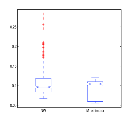
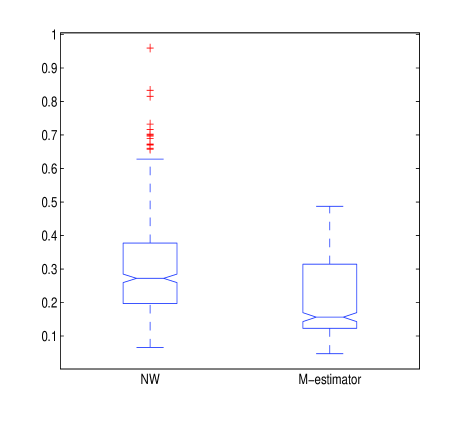
(a) $CR=20\%$	(b) $CR=60\%$

Figure 1: Distribution of the $(MSE_{b})_{b=1,\dots,B}$ obtained from $B=500$ replications using model 1 when $n=300$.

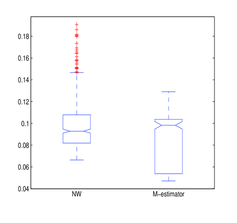
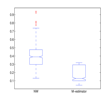
(a) $CR=20\%$	(b) $CR=60\%$

Figure 2: Distribution of the $(MSE_{b})_{b=1,\dots,B}$ obtained from $B=500$ replications using model 1 when $n=800$.

Moreover, in order to provide a deeper analysis of the errors, we consider particularly the model 1 and we plot in Figure 1 and 2 the distribution of the Mean Squared Errors of the two estimators obtained from the $B=500$ replications. As an overall trend, one can see that the $M$-estimator performs better than the NW estimator. This performance decreases when the censoring rate increases.

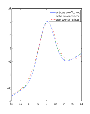
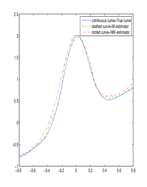
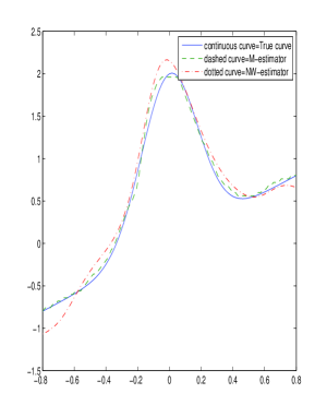
$n=300,CR=20\%$	$n=300,CR=40\%$	$n=300,CR=60\%$

Figure 3: Curves of the true regression function of model 1, $\widehat{\theta}_{\psi,n}(x)$ and $\widehat{\theta}_{n}^{\star}(x)$ obtained when $n=300$ and $CR=20\%,40\%$ and $60\%$ respectively.

In Figures 3 and 4, we plot the true regression function $m(\cdot)$ (from model 1) and its estimators $\widehat{\theta}_{\psi,n}(\cdot)$ and $\widehat{\theta}_{n}^{\star}(\cdot)$ where $\mbox{CR}=20\%,40\%$ and $60\%$ and $n=300$ and $800$ and $h_{n}=n^{-1/3}$. From Figures 3 and 4, it can be seen that, despite the two estimators perform better for bigger sample size $n$ and for small censoring rates, the $M$-estimator stay more accurate than the NW one in all cases. Similar conclusions have been observed for model 2 and model 3.

Here, we want to point out that, although the Kaplan-Meier estimator has some drawback in the edges of the interval, it is nevertheless important of penalized by the survival lae of the censorship r.v. to limit the bad effect in edges. Nevertheless this seems very clear in the usual regression, on the other hand the case of the robust estimator, the effect is very limited by the robust function $\psi$, what appears clearly in Figures 3 and 4.

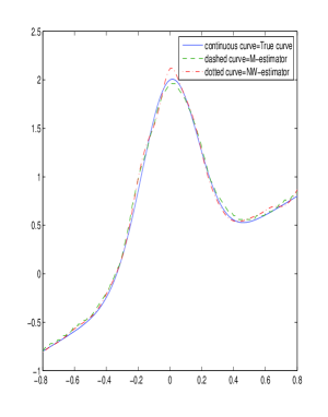
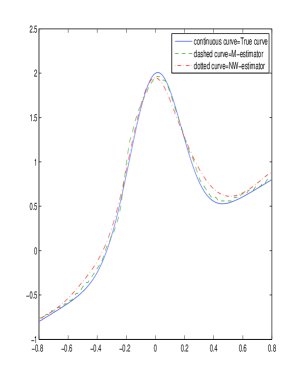
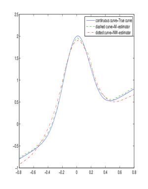
$n=800,CR=20\%$	$n=800,CR=40\%$	$n=800,CR=60\%$

Figure 4: Curves of the true regression function of model 1, $\widehat{\theta}_{\psi,n}(x)$ and $\widehat{\theta}_{n}^{\star}(x)$ obtained when $n=800$ and $CR=20\%,40\%$ and $60\%$ respectively.

4.2 Simulation 2: on the robustness of the $M$-estimator

In this subsection, we are interested in the study of the robustness of the $M$-estimator to the presence of outliers in the data. To reach this purpose, the model 1 is considered and a sample of $n=800$ observations is generated. A percentage of $30\%$ of the data is perturbed by multiplying the original data by a coefficient $k=5,10$ and $20$ respectively. We generate $B=500$ replications and the accuracy of the estimators is measured by the General Mean Square Error. Moreover, the robustness study of $\widehat{\theta}_{\psi,n}$ and $\widehat{\theta}_{n}^{\star}$ has been considered when the censored rate $\mbox{CR}=20\%$ and $60\%$ respectively. One can observe from Table 2 that $M$-estimator is less sensitive to the presence of outliers than the NW-estimator. The sensitivity to outliers of the last estimator increases significantly when the censoring rate increases.

Table 2: The global mean squared errors $\mbox{GMSE}(\widehat{\theta}_{\psi,n})$ and $\mbox{GMSE}(\widehat{\theta}_{n}^{\star})$.

$\mbox{CR}(\%)$	$k$	$\widehat{\theta}_{\psi,n}$	$\widehat{\theta}_{n}^{\star}$
	5	1.78	3.92
20	10	1.84	10.65
	20	1.91	34.01
	5	1.91	4.43
60	10	2.00	11.88
	20	2.01	38.22

5 Proofs

The proof of the results needs somme additional notations. We denote by

$$\overline{\widetilde{\Psi}}_{N}(x,\theta) = \frac{1}{n\mathbb{E}(\Delta_{1}(x))}\sum_{i=1}^{n}\mathbb{E}\left\{\Delta_{i}(x)\frac{\delta_{i}\psi(Y_{i}-\theta)}{\overline{G}(Y_{i})}\mid\mathcal{F}_{i-1}\right\}\quad\mbox{and}$$

$$\overline{\widehat{\Psi}}_{D}(x) = (n\mathbb{E}(\Delta_{1}(x)))^{-1}\sum_{i=1}^{n}\mathbb{E}[\Delta_{i}(x)\mid\mathcal{F}_{i-1}].$$ (5.1)

Define the pseudo conditional bias of $\widetilde{\Psi}_{n}(x,\theta)$ as

$$B_{n}(x,\theta):=\frac{\overline{\widetilde{\Psi}}_{N}(x,\theta)}{\overline{\widehat{\Psi}}_{D}(x)}-\Psi(x,\theta),$$ (5.2)

and let

$$R_{n}(x,\theta) := -B_{n}(x,\theta)[\widehat{\Psi}_{D}(x)-\overline{\widehat{\Psi}}_{D}(x)],$$ (5.3)

$$Q_{n}(x,\theta) := [\widetilde{\Psi}_{N}(x,\theta)-\overline{\widetilde{\Psi}}_{N}(x,\theta)]-\Psi(x,\theta)[\widehat{\Psi}_{D}(x)-\overline{\widehat{\Psi}}_{D}(x)].$$ (5.4)

Therefore, we have from (5), (5.2), (5.3) and (5.4) that :

$$\widetilde{\Psi}_{n}(x,\theta)-\Psi(x,\theta)=B_{n}(x,\theta)+\frac{R_{n}(x,\theta)+Q_{n}(x,\theta)}{\widehat{\Psi}_{D}(x)}.$$ (5.5)

The proof of our results state in section 3, will be split into several lemmas given hereafter.

We begin by the following technical lemma, which plays the same role as Bochner Theorem.

Lemma 5.1

Assume that Assumptions (A1) and (A4) hold true. For any $j\geq 1$, we have

• $\mathbb{E}\left(\Delta_{i}^{j}(x)|\mathcal{F}_{i-1}\right)=c_{0}h_{i,d}(x)b_{n}^{d}d\int_{0}^{1}k^{j}(u)u^{d-1}du$  a.s.
  

• $\mathbb{E}\left(\Delta_{1}^{j}(x)\right)=c_{0}h(x)b_{n}^{d}d\int_{0}^{1}k^{j}(u)u^{d-1}du$.

Proof . Using Assumption (A4) we can write

$$\mathbb{E}\left(\Delta_{i}^{j}(x)|\mathcal{F}_{i-1}\right) = \mathbb{E}\left(k^{j}(\|X_{i}-x\|_{2}/b_{n})|\mathcal{F}_{i-1}\right)$$

$$= \int_{0}^{b_{n}}k^{j}(u/b_{n})d\mathbb{P}^{\mathcal{F}_{i-1}}\left(\|X_{i}-x\|_{2}\leq u\right)$$

$$= \int_{0}^{1}k^{j}(t)d\mathbb{P}^{F_{i-1}}\left(\|X_{i}-x\|_{2}/b_{n}\leq t\right)$$

$$= k^{j}(1)\mathbb{P}_{X_{i}}^{\mathcal{F}_{i-1}}(S_{b_{n},x})-\int_{0}^{1}(k^{j}(u))^{\prime}\mathbb{P}_{X_{i}}^{\mathcal{F}_{i-1}}(S_{ub_{n},x})du.$$

Finally, using Assumption (A1), the proof of the result given by (i) can be concluded. The proof of (ii) follows from part (i) by considering $\mathcal{F}_{i-1}$ the trivial $\sigma$-field.  

The following exponential lemma is a tool that be used when we deal with difference martingale sequences (whose proof can be found in Laïb and Louani (2011)).

Lemma 5.2

( Laïb and Louani (2011)). Let $(Z_{n})_{n\geq 1}$ be a sequence of real martingale differences with respect to the sequence of $\sigma$-fields $(\mathcal{F}_{n}=\sigma(Z_{1},\dots,Z_{n}))_{n\geq 1}$, where $\sigma(Z_{1},\dots,Z_{n})$ is the $\sigma$-filed generated by the random variables $Z_{1},\dots,Z_{n}$. Set $S_{n}=\sum_{i=1}^{n}Z_{i}.$ For any $p\geq 2$ and any $n\geq 1$, assume that there exist some nonnegative constants $\gamma_{6}$ and $d_{n}$ such that

$$\mathbb{E}\left(Z_{n}^{p}\mid\mathcal{F}_{n-1}\right)\leq\gamma_{6}^{p-2}p!d_{n}^{2}\quad\quad\mbox{a.s.}$$ (5.6)

Then, for any $\epsilon>0$, we have

$$\mathbb{P}\left(|S_{n}|>\epsilon\right)\leq 2\exp\left\{-\frac{\epsilon^{2}}{2(D_{n}+\gamma_{6}\epsilon)}\right\},$$

where $D_{n}=\sum_{i=1}^{n}d_{i}^{2}.$

The following lemma gives the convergence rate of the quantity $\widehat{\Psi}_{D}(x)$.

Lemma 5.3

Suppose that Assumptions (A1)-(A4) hold true, then we have

• $\lim_{n\rightarrow\infty}\widehat{\Psi}_{D}(x)=\lim_{n\rightarrow\infty}\overline{\widehat{\Psi}}_{D}(x)=1,\ \ a.s.$

• $\widehat{\Psi}_{D}(x)-\overline{\widehat{\Psi}}_{D}(x)=\mathcal{O}_{a.s.}\left(\sqrt{\displaystyle\frac{\log n}{nb_{n}^{d}}}\right)$.

Proof . First, observe that $\widehat{\Psi}_{D}(x)-1=Z_{n,1}(x)+Z_{n,2}(x)$, where

$$Z_{n,1}(x):=\frac{1}{n\mathbb{E}(\Delta_{1}(x))}\sum_{i=1}^{n}\left(\Delta_{i}(x)-\mathbb{E}(\Delta_{i}(x)|\mathcal{F}_{i-1})\right)$$

and

$$Z_{n,2}(x):=\frac{1}{n\mathbb{E}(\Delta_{1}(x))}\sum_{i=1}^{n}\left[\mathbb{E}(\Delta_{i}(x)|\mathcal{F}_{i-1})-\mathbb{E}(\Delta_{1}(x))\right].$$

It can be easily seen that $\mathbb{E}(\Delta_{i}(x)|\mathcal{F}_{i-1})-\mathbb{E}(\Delta_{1}(x))=c_{0}b_{n}^{d}d\left[h_{i}(x)-h(x)\right]\int_{0}^{1}k(u)u^{d-1}du.$

Then Assumption (A2) combined with Lemma 5.1 allow to conclude that $Z_{n,2}(x)=o(1)$ a.s. as $n\rightarrow\infty.$

To deal with the term $Z_{n,1}(x)$ write it as follows

$$\displaystyle Z_{n,1}(x)=\frac{1}{n}\sum_{i=1}^{n}L_{n,i}(x),$$

with $\displaystyle L_{n,i}(x)=\left[\Delta_{i}(x)-\mathbb{E}(\Delta_{i}(x)|\mathcal{F}_{i-1})\right]/\mathbb{E}(\Delta_{1}(x))$ is a martingale difference.

Now, the consistency of the term $Z_{n,1}(x)$ can follows from the application of Lemma 1 in Chaouch et al. (2013). Therefore, let us check the condition on which this later can be applied.

Observe that

$$|L_{n,i}(x)|=\frac{|\Delta_{i}(x)-\mathbb{E}(\Delta_{i}(x)|\mathcal{F}_{i-1})|}{|\mathbb{E}(\Delta_{1}(x))|}\leq\frac{2\overline{k}}{c_{0}b_{n}^{d}dh(x)\int_{0}^{1}k(u)u^{d-1}du}=:M,$$

where $\overline{k}:=\sup_{x\in\mathbb{R}^{+}}k(x).$

On the other hand, making use of Lemma 5.1, one can see that

$$\mathbb{E}\left(L_{n,i}^{2}(x)|\mathcal{F}_{i-1}\right)=\frac{\int_{0}^{1}k^{2}(u)u^{d-1}du}{c_{0}b_{n}^{d}dh^{2}(x)\left(\int_{0}^{1}k(u)u^{d-1}du\right)^{2}}\ h_{i}(x)=:d_{i}^{2}.$$

Then using Lemma 1 in Chaouch et al. (2013), with $D_{n}=\sum_{i=1}^{n}d_{i}^{2}$, we obtain for any $\lambda>0$

$$\displaystyle\mathbb{P}\left(\frac{1}{n}\Big{|}\sum_{i=1}^{n}L_{n,i}(x)\Big{|}\geq\lambda\right) \leq 2\exp\left\{-\frac{n^{2}\lambda^{2}}{4D_{n}+2Mn\lambda}\right\}$$

$$= \displaystyle 2\exp\left\{-\frac{n\lambda^{2}}{4\frac{D_{n}}{n}+2M\lambda}\right\}.$$

Moreover, using Lemma 5.1, we get $\displaystyle 4\frac{D_{n}}{n}+2M\lambda=\frac{C_{\lambda}(x)}{b_{n}^{d}},$ where

$$C_{\lambda}(x)=\frac{4\left(\int_{0}^{1}k^{2}(u)u^{d-1}du\right)\left(\int_{0}^{1}k(u)u^{d-1}du\right)^{-2}+4\lambda\overline{k}\left(\int_{0}^{1}k(u)u^{d-1}du\right)}{c_{0}dh(x)}.$$

Consequently,

$$\mathbb{P}\left(\frac{1}{n}\Big{|}\sum_{i=1}^{n}L_{n,i}(x)\Big{|}\geq\lambda\right)\leq 2\exp\left\{-\frac{\lambda^{2}}{C_{\lambda}(x)}\ nb_{n}^{d}\right\}.$$

Taking into account the Assumption (A3), the result is concluded by Borel-Cantelli Lemma. The quantity $\overline{\widehat{\Psi}}_{D}(x)$ could be treated in a similar way as $\widehat{\Psi}_{D}(x)$. Concerning the item (ii) one can use same arguments as the study of $Z_{n,1}(x)$.

 

Lemma below establishes the convergence almost surely (with rate) of the conditional bias term $B_{n}$ and the central term $R_{n}$ defined respectively in (5.2) and (5.3).

Lemma 5.4

Assume that Assumptions (A1)-(A4), (A5)(iii) and (A6)(i) hold true, then we get

$$\sup_{\theta\in\mathcal{C}_{\psi,\tau}}|B_{n}(x,\theta)|=\mathcal{O}_{a.s.}(b_{n}^{d\alpha_{1}}),$$ (5.7)

and

$$\sup_{\theta\in\mathcal{C}_{\psi,\tau}}|R_{n}(x,\theta)|=\mathcal{O}_{a.s.}\left(b_{n}^{d\alpha_{1}}\sqrt{\frac{\log n}{nb_{n}^{d}}}\right).$$ (5.8)

Proof . Recall that

$$B_{n}(x,\theta)=\frac{\overline{\widetilde{\Psi}}_{N}(x,\theta)-\overline{\widehat{\Psi}}_{D}(x)\Psi(x,\theta)}{\overline{\widehat{\Psi}}_{D}(x)}.$$

By a double conditioning w.r.t. the $\sigma$-fields $(\mathcal{G}_{i-1},\;T_{i})$ and $\mathcal{F}_{i-1}$, it follows from (A6)(i) that

$$\overline{\widetilde{\Psi}}_{N}(x,\theta) = \frac{1}{n\mathbb{E}(\Delta_{1}(x))}\sum_{i=1}^{n}\mathbb{E}\left\{\Delta_{i}(x)\mathbb{E}\left[\frac{\delta_{i}\,\psi(Y_{i}-\theta)}{\overline{G}(Y_{i})}|\mathcal{G}_{i-1},T_{i}\right]|\mathcal{F}_{i-1}\right\}$$

$$= \frac{1}{n\mathbb{E}(\Delta_{1}(x))}\sum_{i=1}^{n}\mathbb{E}\left\{\Delta_{i}(x)\mathbb{E}\left[\frac{\delta_{i}\,\psi(Y_{i}-\theta)}{\overline{G}(Y_{i})}|X_{i},T_{i}\right]|\mathcal{F}_{i-1}\right\}.$$

Therefore, one gets

$$\overline{\widetilde{\Psi}}_{N}(x,\theta)-\overline{\widehat{\Psi}}_{D}(x)\Psi(x,\theta)=\frac{1}{n\mathbb{E}(\Delta_{1}(x))}\sum_{i=1}^{n}\mathbb{E}\left\{\Delta_{i}(x)\left[\Psi(X_{i},\theta)-\Psi(x,\theta)\right]|\mathcal{F}_{i-1}\right\}.$$

Making use of the triangular inequality and Assumption (A5)(iii) we get

$$\overline{\widetilde{\Psi}}_{N}(x,\theta)-\overline{\widehat{\Psi}}_{D}(x)\Psi(x,\theta)=\mathcal{O}_{a.s.}(b_{n}^{d\alpha_{1}})\times\overline{\widehat{\Psi}}_{D}(x).$$

Finally using Lemma 5.3 we deduce the consistency rate of $B_{n}(x,\theta)$ given by the equation (5.7). Moreover, since $R_{n}(x,\theta)=-B_{n}(x,\theta)[\widehat{\Psi}_{D}(x)-\overline{\widehat{\Psi}}_{D}(x)]$, then equation (5.7) and Lemma 5.3 allow to get the consistency rate of $R_{n}(x,\theta)$ given by the equation (5.8)  

The following lemma deals with the convergence rate of the numerator $\widetilde{\Psi}_{N}(x,\theta)$ defined in (2.6) of the pseudo-estimator $\widetilde{\Psi}_{n}(x,\theta)$.

Lemma 5.5

Under Assumptions (A0)-(A4) and (A5)(iii), we have

$$\sup_{\theta\in\mathcal{C}_{\psi,\tau}}|\widetilde{\Psi}_{N}(x,\theta)-\overline{\widetilde{\Psi}}_{N}(x,\theta)|=\mathcal{O}_{a.s.}\left(\sqrt{\frac{\log n}{nb_{n}^{d}}}\right).$$ (5.9)

Proof . Since $\displaystyle{\cal C}_{\psi,\tau}:=[\theta_{\psi}(x)-\tau,\;\theta_{\psi}(x)+\tau]$ is a compact set, it admits a covering by a finite number $d_{n}$ of balls $\mathcal{B}_{j}(t_{j},\ell_{n})$ centered at $t_{j}$, $1\leq j\leq d_{n}$ satisfies $\ell_{n}=n^{-1/2}$ and $d_{n}=\mathcal{O}(n^{-\alpha_{2}/2})$.

Therefore,

$$\displaystyle\sup_{\theta\in\mathcal{C}_{\psi,\tau}}|\widetilde{\Psi}_{N}(x,\theta)-\overline{\widetilde{\Psi}}_{N}(x,\theta)| \leq \max_{1\leq j\leq d_{n}}\sup_{\theta\in\mathcal{B}_{j}}|\widetilde{\Psi}_{N}(x,\theta)-\widetilde{\Psi}_{N}(x,t_{j})|+\max_{1\leq j\leq d_{n}}|\widetilde{\Psi}_{N}(x,t_{j})-\overline{\widetilde{\Psi}}_{N}(x,t_{j})|$$ (5.10)

$$+\max_{1\leq j\leq d_{n}}\sup_{\theta\in\mathcal{B}_{j}}|\overline{\widetilde{\Psi}}_{N}(x,t_{j})-\overline{\widetilde{\Psi}}_{N}(x,\theta)|$$

$$=: \mathcal{J}_{n,1}+\mathcal{J}_{n,2}+\mathcal{J}_{n,3}.$$

Consistency of the first term $\mathcal{J}_{n,1}$

Using Assumption (A6)(ii), we get

$$\displaystyle|\widetilde{\Psi}_{N}(x,\theta)-\widetilde{\Psi}_{N}(x,t_{j})| \leq \frac{1}{n\mathbb{E}(\Delta_{1}(x))}\sum_{i=1}^{n}\Delta_{i}(x)\frac{\delta_{i}}{\overline{G}(Y_{i})}\left|\psi(Y_{i}-\theta)-\psi(Y_{i}-t_{j})\right|$$

$$\leq \displaystyle\frac{\ell_{n}}{\overline{G}(\tau_{F})}\widehat{\Psi}_{D}(x).$$

Therefore, since (by Lemma 5.3) $\displaystyle\widehat{\Psi}_{D}(x)=\mathcal{O}_{a.s.}(1)$ and $\overline{G}(\tau_{F})>0$, then we have

$$\displaystyle\mathcal{J}_{n,1}=\mathcal{O}_{a.s.}\left(\sqrt{\frac{1}{n}}\right).$$ (5.11)

Consistency of the third term $\mathcal{J}_{n,3}$

Using a double conditioning with respect to the $\sigma$-algebra $\mathcal{G}_{i-1}$ and the definition of $\Psi(x,\theta)$ given by equation (2.4), one can easily obtain

$$\overline{\widetilde{\Psi}}_{N}(x,t_{j})-\overline{\widetilde{\Psi}}_{N}(x,\theta)=\frac{1}{n\mathbb{E}(\Delta_{1}(x))}\sum_{i=1}^{n}\mathbb{E}\left\{\Delta_{i}(x)\left[\Psi(X_{i},t_{j})-\Psi(X_{i},\theta)\right]|\mathcal{F}_{i-1}\right\}.$$

Then using Assumption (A5)(iii) and Lemma 5.3 we have

$$\mathcal{J}_{n,3}=\mathcal{O}_{a.s.}(n^{-\alpha_{2}/2}).$$ (5.12)

Consistency of the second term $\mathcal{J}_{n,2}$

First, observe that $\mathcal{J}_{n,2}$ can be written as

$$\displaystyle\mathcal{J}_{n,2} = \max_{1\leq j\leq d_{n}}\Big{|}\widetilde{\Psi}_{N}(x,t_{j})-\overline{\widetilde{\Psi}}_{N}(x,t_{j})\Big{|}$$

$$= \max_{1\leq j\leq d_{n}}\frac{1}{n\mathbb{E}(\Delta_{1}(x))}\Big{|}\sum_{i=1}^{n}S_{n,i}(x,t_{j})\Big{|},$$

where $S_{n,i}(x,t_{j})=\Delta_{i}(x)\frac{\delta_{i}\,\psi(Y_{i}-t_{j})}{\overline{G}(Y_{i})}-\mathbb{E}\left[\Delta_{i}(x)\frac{\delta_{i}\,\psi(Y_{i}-t_{j})}{\overline{G}(Y_{i})}|\mathcal{F}_{i-1}\right]$ is a martingale difference. Therefore, one can use Lemma 5.2 to obtain an exponential upper bound relative to the quantity $\widetilde{\Psi}_{N}(x,t_{j})-\overline{\widetilde{\Psi}}_{N}(x,t_{j})$.

Let us now check the conditions under which Lemma 5.2 is allowed to be applied. We have, for any $p\in\mathbb{N}-\{0\}$, that

$$S_{n,i}^{p}(x,t_{j})=\sum_{k=0}^{p}C_{p}^{k}\left(\frac{\delta_{i}}{\overline{G}(Y_{i})}\psi(Y_{i}-t_{j})\Delta_{i}(x)\right)^{k}(-1)^{p-k}\left[\mathbb{E}\left(\frac{\delta_{i}}{\overline{G}(Y_{i})}\psi(Y_{i}-t_{j})\Delta_{i}(x)|\mathcal{F}_{i-1}\right)\right]^{p-k}.$$

In view of Assumption (A6)(i), $\left[\mathbb{E}\left(\frac{\delta_{i}}{\overline{G}(Y_{i})}\psi(Y_{i}-t_{j})\Delta_{i}(x)|\mathcal{F}_{i-1}\right)\right]^{p-k}$ is $\mathcal{F}_{i-1}$-measurable. Therefore, using Jensen’s inequality, one gets

$$\Big{|}\mathbb{E}\left(S_{n,i}^{p}(x,t_{j})|\mathcal{F}_{i-1}\right)\Big{|}\leq\sum_{k=0}^{p}C_{p}^{k}\mathbb{E}\left\{\Big{|}\frac{\delta_{i}}{\overline{G}(Y_{i})}\psi(Y_{i}-t_{j})\Delta_{i}(x)\Big{|}^{k}|\mathcal{F}_{i-1}\right\}\times\mathbb{E}\left\{\Big{|}\frac{\delta_{i}}{\overline{G}(Y_{i})}\psi(Y_{i}-t_{j})\Delta_{i}(x)\Big{|}^{p-k}|\mathcal{F}_{i-1}\right\}$$

Using now a double conditioning w.r.t. the $\sigma$-field $\mathcal{G}_{i-1}$, Assumptions (A0) and (A6)(i), we get, for any $m\geq 1$, that

$$\mathbb{E}\left\{\Big{|}\frac{\delta_{i}}{\overline{G}(Y_{i})}\psi(Y_{i}-t_{j})\Delta_{i}(x)\Big{|}^{m}|\mathcal{F}_{i-1}\right\} \leq \frac{1}{(\overline{G}(\tau_{F}))^{m-1}}\mathbb{E}\left\{\Delta_{i}^{m}(x)\mathbb{E}\left[\psi^{m}(Y_{i}-t_{j})|X_{i}\right]|\mathcal{F}_{i-1}\right\}$$

$$\leq \frac{\gamma_{3}m!}{(\overline{G}(\tau_{F}))^{m-1}}\mathbb{E}\left(\Delta_{i}^{m}(x)|\mathcal{F}_{i-1}\right).$$

Making use of Lemma 5.1, we obtain $\mathbb{E}\left(\Delta_{i}^{m}(x)|\mathcal{F}_{i-1}\right)=c_{0}h_{i}(x)db_{n}^{d}\int_{0}^{1}k^{m}(u)u^{d-1}du$. It results then from (A4)(ii) that

$$\mathbb{E}\left(\Big{|}\frac{\delta_{i}\psi(Y_{i}-t_{j})}{\overline{G}(Y_{i})}\Delta_{i}(x)\Big{|}^{k}|\mathcal{F}_{i-1}\right)\;\mathbb{E}\left(\Big{|}\frac{\delta_{i}\psi(Y_{i}-t_{j})}{\overline{G}(Y_{i})}\Delta_{i}(x)\Big{|}^{p-k}|\mathcal{F}_{i-1}\right)\leq\gamma_{3}h_{i}^{2}(x)b_{n}^{2d}.$$

Finally, we have $\Big{|}\mathbb{E}\left(S_{n,i}^{p}(x,t_{j})|\mathcal{F}_{i-1}\right)\Big{|}\leq 2^{p}h_{i}^{2}(x)b_{n}^{d}.$

By taking $d_{i}^{2}=h_{i}^{2}(x)b_{n}^{d}$ and $D_{n}=\sum_{i=1}^{n}d_{i}^{2}=b_{n}^{d}\sum_{i=1}^{n}h_{i}^{2}(x)$, one gets, by Assumption (A2), that $n^{-1}D_{n}=b_{n}^{d}h(x)$ as $n\rightarrow\infty.$ Now one can use Lemma 5.2 with $D_{n}=O_{a.s.}(nb_{n}^{d})$ and $S_{n}=\sum_{i=1}^{n}S_{n,i}(x,t_{j})$ to get, for any $\epsilon_{0}>0,$

$$\mathbb{P}\left(|\mathcal{J}_{n,2}|>\epsilon_{0}\sqrt{\frac{\log n}{nb_{n}^{d}}}\right) \leq \sum_{j=1}^{d_{n}}\mathbb{P}\left(\Big{|}\widetilde{\Psi}_{N}(x,t_{j})-\overline{\widetilde{\Psi}}_{N}(x,t_{j})\Big{|}>\epsilon_{0}\sqrt{\frac{\log n}{nb_{n}^{d}}}\right)$$

$$= \sum_{j=1}^{d_{n}}\mathbb{P}\left(\frac{1}{\mathbb{E}(\Delta_{1}(x))}\Big{|}\sum_{i=1}^{n}S_{n,i}(x,t_{j})\Big{|}>\epsilon_{0}\sqrt{\frac{\log n}{nb_{n}^{d}}}\right)$$

$$\leq \sum_{j=1}^{d_{n}}2\exp\left\{-\frac{(n\mathbb{E}(\Delta_{1}(x))\epsilon_{0})^{2}\frac{\log n}{nb_{n}^{d}}}{2D_{n}+2\gamma_{3}n\mathbb{E}(\Delta_{1}(x))\epsilon_{0}\sqrt{\frac{\log n}{nb_{n}^{d}}}}\right\}$$

$$\leq 2d_{n}\exp\left\{-\gamma_{3}\epsilon_{0}^{2}\log n\right\}$$

$$= n^{-\gamma_{3}\epsilon_{0}^{2}}\;n^{-\alpha_{2}/2}.$$

Consequently, choosing $\epsilon_{0}$ such that, the upper bound becomes a general term of a convergence Riemann series, we get $\displaystyle\sum_{n\geq 1}\mathbb{P}\left(|\mathcal{J}_{n,2}|>\epsilon_{0}\sqrt{\frac{\log n}{nb_{n}^{d}}}\right)<\infty.$ The proof can be achieved by Borel-Cantelli Lemma.  

Lemma below study the uniform asymptotic rate of the quantity $Q_{n}(x,\theta)$.

Lemma 5.6

Under assumptions (A1)-(A4) and (A5)(iii), we have

$$\sup_{\theta\in\mathcal{C}_{\psi,\tau}}|Q_{n}(x,\theta)|=\mathcal{O}_{a.s.}\left(\sqrt{\frac{\log n}{nb_{n}^{d}}}\right).$$ (5.13)

Proof . The proof of this Lemma can easily be obtained from Lemmas 5.3 and 5.5 .  

Proof of Proposition 3.3

Observe that

$$\Big{|}\widehat{\Psi}_{n}(x,\theta)-\widetilde{\Psi}_{n}(x,\theta)\Big{|} \leq \frac{1}{n\mathbb{E}(\Delta_{1}(x))\widehat{\Psi}_{D}(x)}\sum_{i=1}^{n}\Big{|}\Delta_{i}(x)\delta_{i}\psi(Y_{i},\theta)\;\left(\frac{1}{\overline{G}_{n}(Y_{i})}-\frac{1}{\overline{G}(Y_{i})}\right)\Big{|}$$

$$\leq \frac{\sup_{t\in{\cal C}_{\psi,\tau}}|\overline{G}_{n}(t)-\overline{G}(t)|}{\overline{G}_{n}(\zeta)}\;\widetilde{\Psi}_{n}(x,\theta)$$

Since $\overline{G}(\zeta)>0$, in conjunction with the Strong Law of Large Numbers (SLLN) and the Law of the Iterated Logarithm (LIL) on the censoring law (see Deheuvels and Einmahl (2000)), the result is an immediate consequence of decomposition (5.5), Lemmas 5.3, 5.4 and 5.6.  

Proof of Theorem 3.4. Making use of the following decomposition

$$\widehat{\Psi}_{n}(x,\theta)-\Psi(x,\theta) = \left(\widehat{\Psi}_{n}(x,\theta)-\widetilde{\Psi}_{n}(x,\theta)\right)+\left(\widetilde{\Psi}_{n}(x,\theta)-\Psi(x,\theta)\right)$$ (5.14)

$$= \left(\widehat{\Psi}_{n}(x,\theta)-\widetilde{\Psi}_{n}(x,\theta)\right)+B_{n}(x,\theta)+\frac{R_{n}(x,\theta)+Q_{n}(x,\theta)}{\widehat{\Psi}_{D}(x)}.$$

The proof follows then as a consequence of Propostion 3.3, Lemmas 5.3, 5.4 and 5.6

 
Proof of Theorem 3.5. Since, $\Psi(x,\theta_{\psi}(x))=0$ and $\widehat{\Psi}_{n}(x,\widehat{\theta}_{\psi,n}(x))=0$, then the Taylor’s expansion of the function $\Psi(x,\cdot)$ around $\theta_{\psi}(x)$ leads to

$$\widehat{\theta}_{\psi,n}(x)-\theta_{\psi}(x) = \frac{\Psi(x,\widehat{\theta}_{\psi,n}(x))}{\Psi^{\prime}(x,\theta^{\star}_{n})}$$ (5.15)

$$= \frac{\Psi(x,\widehat{\theta}_{\psi,n}(x))-\widehat{\Psi}_{n}(x,\widehat{\theta}_{\psi,n}(x))}{\Psi^{\prime}(x,\theta^{\star}_{n})},$$

where $\theta^{\star}_{n}$ lies between $\widehat{\theta}_{\psi,n}(x)$ and $\theta_{\psi}(x).$ It follows from the Assumption (A6)(ii) that $|\Psi^{\prime}(x,\theta^{\star}_{n})|>\gamma$ and therefore

$$\Big{|}\widehat{\theta}_{\psi,n}(x)-\theta_{\psi}(x)\Big{|}=\mathcal{O}\left(\sup_{\theta\in{\cal C}_{\psi,\tau}}\Big{|}\widehat{\Psi}_{n}(x,\theta)-\Psi(x,\theta)\Big{|}\right).$$ (5.16)

The proof of Theorem 3.5 can be then deduced from Theorem 3.4.  

Proof of Theorem 3.7. The proof is based on the following decomposition

$$\left(nb_{n}^{d}\right)^{1/2}\left[\widehat{\Psi}_{n}(x,\theta)-\Psi(x,\theta)\right]$$

$$= \left(nb_{n}^{d}\right)^{1/2}\left[\left(\widehat{\Psi}_{n}(x,\theta)-\widetilde{\Psi}_{n}(x,\theta)\right)+\left(\widetilde{\Psi}_{n}(x,\theta)-\overline{\widetilde{\Psi}}_{n}(x,\theta)\right)+\left(\overline{\widetilde{\Psi}}_{n}(x,\theta)-\Psi(x,\theta)\right)\right]$$

$$=: \mathcal{L}_{1,n}+\mathcal{L}_{2,n}+\mathcal{L}_{3,n}.$$

By Proposition 3.3 and assumption (A3)(ii), we have $\mathcal{L}_{1,n}=\mathcal{O}_{a.s.}\left(nb_{n}^{d}\sqrt{\log\log n/n}\right)=o_{a.s.}(1)$. The term $\mathcal{L}_{n,3}$ is equal to $\sqrt{nb_{n}^{d}}B_{n}(x,\theta)$ which is $o_{a.s.}(1)$ in view of assumption (A3)(ii) and Lemma (5.4). Moreover, observe that $\mathcal{L}_{n,2}=\sqrt{nb_{n}^{d}}\left(Q_{n}(x,\theta)-R_{n}(x,\theta)\right)/\widehat{\Psi}_{D}(x)$. The quantity $\sqrt{nb_{n}^{d}}R_{n}(x,\theta)$ converges almost surely to zero when $n$ goes to infinity, using the second part of Lemma 5.4 combined with assumption (A3)(ii). Moreover, since by Lemma 5.3, $\lim_{n\rightarrow\infty}\widehat{\Psi}_{D}(x)=1$ almost surely, then using Slutsky’s Theorem, the asymptotic normality is given by the central term $\sqrt{nb_{n}^{d}}Q_{n}(x,\theta)$ which is the subject of the following Lemma 5.7.  

Lemma 5.7

Suppose that Assumptions (A1)-(A8) are satisfied, then we have

$$\left(nb_{n}^{d}\right)^{1/2}Q_{n}(x,\theta)\stackrel{{\scriptstyle\mathcal{D}}}{{\longrightarrow}}\mathcal{N}(0,\sigma^{2}(x,\theta)),\quad\quad\mbox{as}\;\;n\rightarrow\infty,$$

where $\sigma^{2}(x,\theta)$ is defined in Theorem 3.7.

Proof . Let us consider

$$\eta_{ni}=\left(\frac{b_{n}^{d}}{n}\right)^{1/2}\left(\frac{\delta_{i}}{\overline{G}(Y_{i})}\psi(Y_{i}-\theta)-\Psi(x,\theta)\right)\frac{\Delta_{i}(x)}{\mathbb{E}(\Delta_{1}(x))}$$

and define $\xi_{ni}=\eta_{ni}-\mathbb{E}(\eta_{ni}|\mathcal{F}_{i-1})$. One can see that

$$(nb_{n}^{d})^{1/2}Q_{n}(x,\theta)=\sum_{i=1}^{n}\xi_{ni},$$ (5.17)

where, for any fixed $x\in\mathbb{R}^{d}$, the summands in (5.17) form a triangular array of stationary martingale differences with respect to $\sigma$-field $\mathcal{F}_{i-1}$. This allows us to apply the Central Limit Theorem for discrete-time arrays of real-valued martingales (as given in Hall and Heyde (1980), page 23) to establish the asymptotic normality of $Q_{n}(x,\theta)$. Therefore, we have to establish the following statements:

• $\sum_{i=1}^{n}\mathbb{E}[\xi_{ni}^{2}|\mathcal{F}_{i-1}]\stackrel{{\scriptstyle\mathbb{P}}}{{\longrightarrow}}\sigma^{2}(x,\theta),$

• $n\mathbb{E}[\xi_{ni}^{2}1\kern-1.99997pt{\rm l}_{[|\xi_{ni}|>\epsilon]}]=o(1)$ holds for any $\epsilon>0$ (Lindberg condition).

Proof of part (a). Observe that

$$\left|\sum_{i=1}^{n}\mathbb{E}[\eta_{ni}^{2}|\mathcal{F}_{i-1}]-\sum_{i=1}^{n}\mathbb{E}[\xi_{ni}^{2}|\mathcal{F}_{i-1}]\right|\leq\sum_{i=1}^{n}\left(\mathbb{E}[\eta_{ni}|\mathcal{F}_{i-1}]\right)^{2}.$$

By double conditioning with respect to ($\mathcal{G}_{i-1},T_{i})$ and ${\cal F}_{i-1}$ and using Assumptions (A2) and (A5)(iii) and Lemma 5.1, we obtain

$$\sum_{i=1}^{n}\left(\mathbb{E}[\eta_{ni}|\mathcal{F}_{i-1}]\right)^{2}=\mathcal{O}_{a.s.}\left(b_{n}^{(2\alpha_{1}+1)d}\right).$$ (5.18)

Therefore, the statement of (a) follows then if we show that

$$\lim_{n\rightarrow\infty}\sum_{i=1}^{n}\mathbb{E}[\eta_{ni}^{2}|\mathcal{F}_{i-1}]\stackrel{{\scriptstyle\mathbb{P}}}{{\longrightarrow}}\sigma^{2}(x,\theta).$$ (5.19)

To prove (5.19), observe that (by double conditioning) that

$$\sum_{i=1}^{n}\mathbb{E}[\eta_{ni}^{2}|\mathcal{F}_{i-1}]=\frac{b_{n}^{d}/n}{(\mathbb{E}(\Delta_{1}(x)))^{2}}\sum_{i=1}^{n}\mathbb{E}\left\{\Delta_{i}^{2}(x)\mathbb{E}\left[\left(\frac{\delta_{i}}{\overline{G}(Y_{i})}\psi(Y_{i}-\theta)-\Psi(x,\theta)\right)^{2}|X_{i}\right]|\mathcal{F}_{i-1}\right\}.$$

Using the definition of the conditional variance, one gets

$$\mathbb{E}\left[\left(\frac{\delta_{i}\psi(Y_{i}-\theta)}{\overline{G}(Y_{i})}-\Psi(x,\theta)\right)^{2}|X_{i}\right] = \mbox{Var}\left\{\frac{\delta_{i}\psi(Y_{i}-\theta)}{\overline{G}(Y_{i})}|X_{i}\right\}+\left\{\mathbb{E}\left(\frac{\delta_{i}\psi(Y_{i}-\theta)}{\overline{G}(Y_{i})}|X_{i}\right)-\Psi(x,\theta)\right\}^{2}$$

$$= \mathcal{K}_{n,1}+\mathcal{K}_{n,2}.$$

Using again a double conditioning with respect to $({\cal G}_{i-1},T_{i})$, Assumptions (A5)(iii) and (A2) and Lemma 5.1, we obtain

$$\frac{b_{n}^{d}/n}{(\mathbb{E}(\Delta_{1}(x)))^{2}}\sum_{i=1}^{n}\mathbb{E}[\Delta_{i}^{2}(x)\mathcal{K}_{n,2}|\mathcal{F}_{i-1}]=\mathcal{O}_{a.s.}\left(b_{n}^{2\alpha_{1}d}\right).$$

Similarly one can show, by Assumptions (A2), (A3), (A5)(iii), (A7) and Lemma 5.1, that

$$\lim_{n\rightarrow\infty}\frac{b_{n}^{d}/n}{(\mathbb{E}(\Delta_{1}(x)))^{2}}\sum_{i=1}^{n}\mathbb{E}[\Delta_{i}^{2}(x)\mathcal{K}_{n,1}|\mathcal{F}_{i-1}] = \left(\mathbb{M}(x,\theta)-\Psi(x,\theta)\right)\times\frac{\int_{0}^{1}k^{2}(u)u^{d-1}du}{h(x)d\left(\int_{0}^{1}k(u)u^{d-1}du\right)^{2}}$$

$$=: \sigma^{2}(x,\theta).$$

Proof of part (b)

The Lindeberg’s condition results from Corollary 9.5.2 in Chow and Teicher (1998) which implies that

$$n\mathbb{E}\left[\xi_{ni}^{2}1\kern-1.99997pt{\rm l}_{[|\xi_{ni}|>\epsilon]}\right]\leq 4n\mathbb{E}\left[\eta_{ni}^{2}1\kern-1.99997pt{\rm l}_{[|\eta_{ni}|>\epsilon/2]}\right].$$

Let $a>1$ and $b>1$ such that $1/a+1/b=1$. Making use of Hölder and Markov inequalities one can write, for all $\epsilon>0$ $\mathbb{E}[\eta_{ni}^{2}1\kern-1.99997pt{\rm l}_{[|\eta_{ni}|>\epsilon/2]}]\leq\frac{\mathbb{E}|\eta_{ni}|^{2a}}{(\epsilon/2)^{2a/b}}$. Taking $C_{0}$ a positive constant and $2a=2+\varsigma$, one gets by Assumption (A8) that

$$4n\mathbb{E}\left[\eta_{ni}^{2}1\kern-1.99997pt{\rm l}_{[|\eta_{ni}|>\epsilon/2]}\right] \leq C_{0}\left(\frac{b_{n}^{d}}{n}\right)^{(2+\varsigma)/2}\frac{n\mathbb{E}[\Delta_{1}^{2+\varsigma}(x)]}{\left(\mathbb{E}(\Delta_{1}(x))\right)^{2+\varsigma}}\;\;[\widetilde{\mathbb{V}}_{2+\varsigma}(\theta|x)+o(1)].$$

Finally Lemma 5.1 allows one to write that $4n\mathbb{E}\left[\eta_{ni}^{2}1\kern-1.99997pt{\rm l}_{[|\eta_{ni}|>\epsilon/2]}\right]=\mathcal{O}_{a.s.}\left(\left(nb_{n}^{d}\right)^{-\varsigma/2}\right)$ which complete the proof by using Assumption (A3).  

Proof of Theorem 3.8. Using a Taylor’s expansion of order one of $\widehat{\Psi}_{n}(x,\cdot)$ around $\theta_{\psi}(x)$ and the definition of $\theta_{\psi}(x)$, we get

$$\widehat{\Psi}_{n}(x,\theta_{\psi}(x))-\Psi(x,\theta_{\psi}(x))=\left(\theta_{\psi}(x)-\widehat{\theta}_{\psi,n}(x)\right)\widehat{\Psi}_{n}^{\prime}(x,\theta^{\star}_{n})$$

where $\theta^{\star}_{n}$ lies between $\theta_{\psi}(x)$ and $\widehat{\theta}_{\psi,n}(x).$ Then, we have

$$\widehat{\theta}_{\psi,n}(x)-\theta_{\psi}(x)=-\frac{\widehat{\Psi}_{n}(x,\theta_{\psi}(x))-\Psi(x,\theta_{\psi}(x))}{\widehat{\Psi}_{n}^{\prime}(x,\theta^{\star}_{n})}.$$

Therefore, the asymptotic normality given by Theorem 3.8 can be stated using Theorem 3.7 and the following lemma which provides the convergence in probability of the denominator term $\widehat{\Psi}_{n}^{\prime}(x,\theta^{\star}_{n})$ to $\Gamma_{1}(x,\theta_{\psi}(x))$.  

Lemma 5.8

Under assumptions of Theorem 3.8, we have, uniformly in $\theta$,

$$\widehat{\Psi}_{n}^{\prime}(x,\theta)\rightarrow\Gamma_{1}(x,\theta)\;\;\mbox{in probablility as}\;\;n\rightarrow\infty.$$

Proof . The proof of this lemma is based on the following decomposition

$$|\widehat{\Psi}_{n}^{\prime}(x,\theta^{\star})-\Gamma_{1}(x,\theta(x))|\leq|\widehat{\Psi}_{n}^{\prime}(x,\theta^{\star})-\widehat{\Psi}_{n}^{\prime}(x,\theta(x))|+|\widehat{\Psi}_{n}^{\prime}(x,\theta(x))-\Gamma_{1}(x,\theta(x))|$$ (5.20)

Concerning the first term, using the fact that $\delta_{i}$ is bounded by one and $\overline{G}_{n}(Y_{i})$ is dominated by $\overline{G}_{n}(\zeta)$, then one can write

$$|\widehat{\Psi}_{n}^{\prime}(x,\theta^{\star})-\widehat{\Psi}_{n}^{\prime}(x,\theta_{\psi}(x))|\leq\sup_{t\in\mathcal{C}_{\psi,\tau}}\left|\frac{\partial\psi(t-\theta^{\star})}{\partial\theta}-\frac{\partial\psi(t-\theta_{\psi}(x))}{\partial\theta}\right|\;\frac{1}{\overline{G}_{n}(\zeta)}.$$

Because $\partial\psi(T-\theta)/\partial\theta$ is continuous at $\theta_{\psi}(x)$ uniformly in $t$, the use of Theorem 3.5 and the convergence in probability of $\overline{G}_{n}(\zeta_{F})$ to $\overline{G}(\tau_{F})$ allows to conclude that the first term of (5.20) converges in probability to zero.

Considering Assumptions (A1)-(A4), (A5)(iii) and (A6)(i), one can show, by using similar arguments as in the proof of Lemma 5.4, that the second term in the right side of the inequality (5.20) converges almost surely to zero.  

Proof of Corollary 3.9. Observe that

$$\widehat{\Gamma}_{1,n}(x,\widehat{\theta}_{\psi,n}(x))\left\{\frac{n\;\widehat{\mathbb{P}}_{X_{i}}(S_{b_{n},x})\;d}{\widehat{\mathbb{M}}_{n}(x,\widehat{\theta}_{\psi,n}(x))\int_{0}^{1}k^{2}(u)u^{d-1}du}\right\}^{1/2}\int_{0}^{1}k(u)u^{d-1}du\times\left(\widehat{\theta}_{\psi,n}(x)-\theta_{\psi}(x)\right) =$$

$$\left\{\frac{\widehat{\mathbb{P}}_{X_{i}}(S_{b_{n},x})}{b_{n}^{d}h(x)}\right\}^{1/2}\left\{\frac{\mathbb{M}(x,\theta_{\psi}(x))}{\widehat{\mathbb{M}}_{n}(x,\widehat{\theta}_{\psi,n}(x))}\right\}^{1/2}\left\{\frac{\widehat{\Gamma}_{1,n}(x,\widehat{\theta}_{\psi,n}(x))}{\Gamma_{1}(x,\theta_{\psi}(x))}\right\} \times$$

$$\Gamma_{1}(x,\theta_{\psi}(x))\left\{\frac{nb_{n}^{d}h(x)d}{\mathbb{M}(x,\theta_{\psi}(x))\int_{0}^{1}k^{2}(u)u^{d-1}du}\right\}^{1/2}\int_{0}^{1}k(u)u^{d-1}du\times\left(\widehat{\theta}_{\psi,n}(x)-\theta_{\psi}(x)\right).$$

Making use of Theorem 3.8, we get

$$\Gamma_{1}(x,\theta_{\psi}(x))\left\{\frac{nb_{n}^{d}h(x)d}{\mathbb{M}(x,\theta_{\psi}(x))\int_{0}^{1}k^{2}(u)u^{d-1}du}\right\}^{1/2}\int_{0}^{1}k(u)u^{d-1}du\times\left(\widehat{\theta}_{\psi,n}(x)-\theta_{\psi}(x)\right)\stackrel{{\scriptstyle\mathcal{D}}}{{\longrightarrow}}\mathcal{N}(0,1).$$

Therefore, the Corollary 3.9 is established if we show that

$$\left\{\frac{\widehat{\mathbb{P}}_{X_{i}}(S_{b_{n},x})}{b_{n}^{d}h(x)}\right\}^{1/2}\left\{\frac{\mathbb{M}(x,\theta_{\psi}(x))}{\widehat{\mathbb{M}}_{n}(x,\widehat{\theta}_{\psi,n}(x))}\right\}^{1/2}\left\{\frac{\widehat{\Gamma}_{1,n}(x,\widehat{\theta}_{\psi,n}(x))}{\Gamma_{1}(x,\theta_{\psi}(x))}\right\}\stackrel{{\scriptstyle\mathbb{P}}}{{\longrightarrow}}1,\quad\mbox{as}\;\;n\rightarrow\infty.$$

By the consistency of the empirical distribution function of $X$ and the decomposition given by (3.2), one obtains

$$\frac{\widehat{\mathbb{P}}_{X_{i}}(S_{b_{n},x})}{b_{n}^{d}h(x)}\stackrel{{\scriptstyle\mathbb{P}}}{{\longrightarrow}}1,\quad\mbox{as}\;\;n\rightarrow\infty.$$

Since $\widehat{\theta}_{\psi,n}(x)$ is a consistent estimator of $\theta_{\psi}(x)$ (see Theorem 3.5), then it suffices to show that $\widehat{\mathbb{M}}_{n}(x,\theta)\stackrel{{\scriptstyle\mathbb{P}}}{{\longrightarrow}}\mathbb{M}(x,\theta)\quad\mbox{and}\quad\widehat{\Gamma}_{1,n}(x,\theta)\stackrel{{\scriptstyle\mathbb{P}}}{{\longrightarrow}}\Gamma_{1}(x,\theta)\;\;\mbox{as}\;\;n\rightarrow\infty$ which are consequence of the previous results.

References

• Azzedine et al. (2008) Azzedine, N., Laksaci, A. and Ould SaΓ―d, E. (2008). On robust nonparametric regression estimation for a functional regressor. Statist. Probab. Lett., 78, 18, 3216–3221.
• Beran (1981) Beran, R. 1981. Nonparametric Regression with Randomly Censored Survival Data. Technical Report. University of California, Berkeley.
• Boente and Fraiman (1989) Boente, G. and Fraiman, R. (1989). Robust nonparametric regression estimation for dependent observations. Ann. Statist., 17, 1242–1256.
• Boente and Fraiman (1990) Boente, G. and Fraiman, R. (1990). Asymptotic distribution of robust estimators for nonparametric models from mixing processes. Ann. Statist., 18, 891–906.
• Boente and Rodriguez (2006) Boente, G. and Rodriguez, D. (2006). Robust estimators of high order derivatives of regression function. Statist. Probab. Lett., 7, 1335–1344.
• Buckley and James (1979) Buckley, J. and James, I. (1979). Linear regression with censored data. Biometrika 66, 429–436.
• Cai and Roussas (1992) Cai, Z.W., and Roussas, G.G. (1992). Uniform strong estimation under $\alpha$-mixing, with rates. Statist. Probab. Lett., 15, 47–55.
• Carbonez el al. (1995) Carbonez, A., GyΓΆrfi, L., and vanΒ der Meulen, E.C. (1995). Partitioning-estimates of a regression function under random censoring. Statist. Decisions, 13, 21–37.
• Chaouch et al. (2013) Chaouch, M., LaΓ―b, N. and Louani, D. (2013). Rate of uniform consistency for a class of mode regression on functional stationary ergodic data. Application to electricity consumption. arXiv:1407.1991.
• Chaouch and Khardani (2013) Chaouch, M., and Khardani, S. (2013). Randomly censored regression quantile estimation using functional stationary ergodic data. To appear, J. Nonparametr. Stat.. DOI: 10.1080/10485252.2014.982651
• Chow and Teicher (1998) Chow, Y., and Teicher, H., Probability Theory, 2nd ed., New York: Springer (1998).
• Collomb and HΓ€rdle (1986) Collomb, G. and HΓ€rdle, W. (1986). Strong uniform convergence rates in robust nonparametric time series analysis and prediction: kernel regression estimation from dependent observations. Stochastic Processes and Applications, 23, 77–89.
• Crambes et al. (2008) Crambes, C. and Delsol, L. and Laksaci, A. (2008). Robust nonparametric estimation for functional data. J. Nonparametr. Stat., 20, 7, 573–598.
• Cox (1972) Cox, D.R. (1972). Regression models and life-tables (with discussion). J. R. Stat. Soc. Ser. B Stat. Methodol. 34, 187–220.
• Dabrowska, D.M. (1987) Dabrowska, D.M. (1987). Nonparametric regression with censored survival data. Scand. J. Statist. 14, 181–197.
• Dabrowska, D.M. (1989) Dabrowska, D.M. (1989). Uniform consistency of the kernel conditional Kaplan-Meier estimate. Ann. Statist. 17, 1157–1167.
• Deheuvels and Einmahl (2000) Deheuvels P. and Einmahl, J.H.J. (2000). Functional limit laws for the increments of Kaplan-Meier product-limit processes and applications. Ann. Probab., 28, 1301–1335.
• Gueriballah et al. (2013) Gheriballah, A., Laksaci, A. and Sekkal, S. (2013) Nonparametric $M$-regression for functional ergodic data. Statist. Probab. Lett., 83, 902–908.
• Guessoum and Ould SaΓ―d (2008) Guessoum, Z. and Ould SaΓ―d, E. (2008). On nonparametric estimation of the regression function under random censorship model. Statist. & Decisions, 26, 159–177.
• Guessoum and Ould SaΓ―d (2012) Guessoum, Z. and Ould SaΓ―d, E. (2012). Central limit theorem for the kernel estimator of the regression function for censored time series. J. Nonparametric Statist., 24, 379–397.
• HΓ€rdle (1984) HΓ€rdle, W. (1984). Robust regression function estimation. J. Multivariate Anal., 14, 169–180.
• Huber (1964) Huber, R.J. (1964). Robust estimation of a location parameter. Ann. Math. Statist., 35, 73–101.
• Hall and Heyde (1980) Hall, P., and Heyde, C.C., Martingale limit theory and its application, Probability and Mathematical Statistics, New York: Academic Press (1980).
• Jin (2007) Jin, Z. (2007). $M$-estimation in regression modes for censored data. J. Statist. Plann. Inference, 12, 3894–3903.
• Kaplan and Meier (1958) Kaplan, E.M. and Meier, P. (1958). Nonparametric estimation from incomplete observations. J. Am. Stat. Assoc., 53, 457–481.
• Khardani el al. (2010) Khardani, S., Lemdani, M., and Ould SaΓ―d, E. (2010). Some asymptotic properties for a smooth kernel estimator of the conditional mode under random censorship. J. Korean Statist. Soc., 39, 455–469.
• Kohler et al. (2002) Kohler, M., MΓ‘thΓ©, K., and PintΓ©r, M. (2002). Prediction from randomly right censored data. J. Multivariate Anal., 80, 73–100.
• Koul and Stute (1998) Koul, H. and Stute, W. (1998). Regression model fitting with long memory errors. J. Statist. Plann. Inference, 71, 35–56.
• Koul et al. (1981) Koul, H., Susarla, V. and Van Ryzin, J. (1981) Regression analysis with randomly right-censored data. Ann. Statist. 9, 1276–1288.
• Krengel (1985) Krengel, U. (1985). Ergodic theorems, Walter de Gruyter & Co. Berlin.
• LaΓ―b (2005) LaΓ―b, N. (2005). Kernel estimates of the mean and the volatility functions in a nonlinear autoregressive model with ARCH errors. J. Statist. Plann. Inference, 134(1), 116–139.
• LaΓ―b and Ould SaΓ―d (2000) LaΓ―b, N. and Ould SaΓ―d, E. (2000). A robust nonparametric estimation of the autoregression function under ergodic hypothesis. Canad. J. Statist., 28, 817–828.
• LaΓ―b and Louani (2010) LaΓ―b, N. and Louani, D. (2010). Nonparametric kernel regression estimation for functional stationary ergodic data: asymptotic properties. J. Multivariate Anal., 101(10), 2266–2281.
• LaΓ―b and Louani (2011) LaΓ―b, N. and Louani, D. (2011). Rates of strong consistencies of the regression function estimator for functional stationary ergodic data. J. Statist. Plann. Inference, 141(1), 359–372.
• Lemdani and Ould SaΓ―d (2013) Lemdani, M. and Ould SaΓ―d, E. (2013) Nonparametric robust regression estimation for censored data. technical report, $n^{0}\;489$, LMPA, ULCO.
• Lipsitz and Ibrahim (2000) Lipsitz, S.R. and Ibrahim, J.G. (2000). Estimation with Correlated Censored Survival Data with Missing Covariates. Biostatistics, 1, 315–327.
• Lu (1999) Lu, Z. Q. (1999). Nonparametric regression with singular design. J. Multivariate Anal., 70, 177–201.
• Ould SaΓ―d and Lamdani (2006) Ould SaΓ―d, E., and Lemdani, M. (2006) Asymptotic properties of a nonparametric regression function estimator with randomly truncated data. Ann. Inst. Statist. Math., 58, 357–378.
• Ren and Gu (1997) Ren, J.J. and Gu, M. (1997). Regression M-estimators with doubly censored data. Ann. Statist., 25, 2638–2664.
• Rosenblatt (1972) Rosenblatt, M. (1972). Uniform ergodicity and strong mixing. Z. Wahrscheinlichkeitstheorie, 24, 79–84.
• Serfling (1980) Serfling, R.J. (1980). Approximation Theorems of Mathematical Statistics, Wiley, New York.
• Wang and Liang (2012) Wang, J.F., and Liang, H.Y. (2012). Asymptotic properties for an M-estimator of the regression function with truncation and dependent data. J. Korean Statist. Soc. 41, 351–367.
• Wei et al. (1989) Wei, L.J., Lin, D.Y. and Weissfeld, L. (1989). Regression analysis of multivariate incomplete failure time data by modeling marginal distributions. J. Amer. Statist. Assoc., 84, 1065–1073