Convolutional Neural Networks for Attribute-based Active Authentication On Mobile Devices

Abstract

We present a Deep Convolutional Neural Network (DCNN) architecture for the task of continuous authentication on mobile devices. To deal with the limited resources of these devices, we reduce the complexity of the networks by learning intermediate features such as gender and hair color instead of identities. We present a multi-task, part-based DCNN architecture for attribute detection that performs better than the state-of-the-art methods in terms of accuracy. As a byproduct of the proposed architecture, we are able to explore the embedding space of the attributes extracted from different facial parts, such as mouth and eyes, to discover new attributes. Furthermore, through extensive experimentation, we show that the attribute features extracted by our method outperform the previously presented attribute-based method and a baseline LBP method for the task of active authentication. Lastly, we demonstrate the effectiveness of the proposed architecture in terms of speed and power consumption by deploying it on an actual mobile device.

Index terms

attributes, face, active authentication, smartphones, mobile, deep networks

1 Introduction

Mobile devices, such as cellphones, tablets, and smart watches have become inseparable parts of people’s lives. The users often store important information such as bank account details or credentials to access their sensitive accounts on their mobile phones. According to the survey in [15], nearly half of the users do not use any form of authentication mechanism for their phones because of the frustrations made by these methods. Even if they do, the initial password-based authentication can be compromised and thus it cannot continuously protect the personal information of the users.

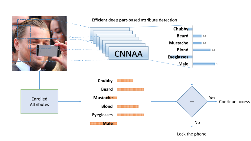
Figure 1: The overview of our method. To authenticate the users, we extract facial attributes by extracting the face parts and feeding them to Convoulutional Neural Network for facial Attribute-based Acitve authentication CNNAA, which is an ensemble of efficient multi-task DCNNs.

To mitigate this issue and make mobile devices more secure, different active authentication (AA) methods have been proposed over the past five years to continuously authenticate the user after he/she unlocks the device. [12], [11], [38], and [3] proposed to continuously authenticate the users based on their touch gestures or swipes. Gait as well as device movement patterns measured by the smartphone accelerometer were used in [8], [41], [27] for continuous authentication. Stylometry, GPS location, web browsing behavior, and application usage patterns were used in [13] for active authentication. Face-based continuous user authentication on mobile devices has also been proposed in [14], [10], [23], and [28, 29]. Different modalities such as speech [23], Gait [7], touch [37] have been fused with faces.

State-of-the-art methods for face recognition employ Deep Convolutional Neural Networks (DCNN) [34], [25], [31], [32]. The previously proposed architectures have many parameters to account for the huge variabilities of facial identities in different conditions. Thus they are not efficient to be used on mobile devices. For instance, it has been shown in [30] that DCNN with an architecture similar to AlexNet [18] can drain the battery very fast.

Facial attributes are also referred to as “soft biometrics” in the literature [16], and a few of them were used in [24] to boost the continuous authentication performance. The recent method of Attribute-based Continuous Authentication (ACA) [28, 29] shows that large number of attributes can give good authentication results on mobile phones on their own. They are semantic features which are easier to learn than facial identities. Also, if they are learned on facial parts, they become less complex. By leveraging these two qualities, we design efficient CNN architectures suitable for mobile devices. As for many other tasks, CNNs are proved to be very accurate for attribute detection [21], [40], [20]. The overview of our method is presented in Figure 1.

The main contribution of this paper is the design of feasible deep architectures for continuous authentication on mobile devices. We also obtain state-of-the-art results from the proposed multi-task, part-based deep architecture for the task of facial attribute extraction. We show that unsupervised subspace clustering of the shared embeddings gathers the semantically related attributes in the same cluster. In addition, we show improvements in attribute-based AA on two publicly available mobile datasets using the attributes from our approach and also the “discovered” attributes by clustering. Finally, we demonstrate the feasibility of the proposed method for mobile devices by testing the speed and power usage calculations on a commercial mobile device.

The rest of this paper is organized as follows. We present the attribute detection models in Section 2. In Section 3, we show that the learned attribute models are effective for active authentication. In Section 4, we evaluate the performance of the proposed architecture using a generic Android device.

2 Attributes

In the mobile setting, there is a trade-off between hardware constraints such as battery life, and accuracy of the models. We design our models with the goal of balancing this trade-off. To do so, we move from a computationally expensive but specialized models to a computationally cheaper but adequately accurate model.

Attribute	DeepMulti-CNNAA	WideMulti-CNNAA	DeepBinary-CNNAA	WideBinary-CNNAA	FaceTracer	PANDA	LNet+ANet
5 o Clock Shadow	93	93	91	89	85	88	91
Arched Eyebrows	81	82	82	83	76	78	79
Attractive	81	81	81	82	78	81	81
Bags Under Eyes	83	84	83	82	76	79	79
Bald	99	99	96	98	89	96	98
Bangs	95	95	94	94	88	92	95
Big Lips	67	70	69	67	64	67	68
Big Nose	82	83	78	78	74	75	78
Black Hair	86	86	88	87	70	85	88
Blond Hair	95	95	94	94	80	93	95
Blurry	95	95	92	80	81	86	84
Brown Hair	86	86	86	84	60	77	80
Bushy Eyebrows	92	92	89	89	80	86	90
Chubby	95	95	87	91	86	86	91
Double Chin	96	96	89	93	88	88	92
Eyeglasses	99	99	99	99	98	98	99
Goatee	97	97	93	96	93	93	95
Gray Hair	98	98	92	97	90	94	97
Heavy Makeup	90	90	90	91	85	90	90
High Cheekbones	86	85	87	87	84	86	87
Male	98	97	97	98	91	97	98
Mouth Slightly Open	93	93	94	94	87	78	92
Mustache	97	96	88	95	91	87	95
Narrow Eyes	87	87	83	81	82	73	81
No Beard	95	95	95	96	90	75	95
Oval Face	72	73	73	70	64	72	66
Pale Skin	97	97	93	94	83	84	91
Pointy Nose	75	73	75	74	68	76	72
Receding Hairline	92	92	88	90	76	84	89
Rosy Cheeks	94	94	87	91	84	73	90
Sideburns	95	95	95	96	94	76	96
Smiling	92	92	92	92	89	89	92
Straight Hair	79	79	78	79	63	73	73
Wavy Hair	71	73	82	81	73	75	80
Wearing Earrings	83	84	86	79	73	92	82
Wearing Hat	98	98	98	98	89	82	99
Wearing Lipstick	92	92	93	93	89	93	93
Wearing Necklace	86	86	71	71	68	86	71
Wearing Necktie	95	96	93	95	86	79	93
Young	87	87	87	88	80	82	87
Average	89.4	89.5	87.7	87.9	81.1	83.6	87.3

Table 1: The accuracy comparison of attribute detection methods. Our multi-task part-based architectures perform better than previously proposed methods and also single-task networks.

We train and test four different sets of DCNNs, in total 100 of them, for the task of attribute classification on a set of face regions. We crop the functional face regions using landmarks detected by [4]. These face regions can be seen in Table 3. For each part, first we find the maximum size of the window in the training dataset, then we crop the regions by putting the center of the face part at the center of the cropped window to avoid any scaling.

2.1 Network architecture

The two proposed architectures of the Deep Convolutional Neural Network for facial Attribute-based Active authentication (Deep-CNNAA) and Wide-CNNAA can be found in Table 2. The four sets of models compared are: BinaryDeep-CNNAA and BinaryWide-CNNAA, which are single task networks, MultiDeep-CNNAA and MultiWide-CNNAA, which are multi-task networks. First we describe the shared configuration that is used to train these networks and then the ones that are specific to each type.

*Wide-CNNAA		*Deep-CNNAA
input	$w\times h\times 3$	input	$w\times h\times 3$
type	patch size	type	patch size
conv_relu	$7\times 7\times 128$	conv_relu	$7\times 7\times 32$
maxpool $3\times 3/2$(stride)
conv_relu	$5\times 5\times 128$	conv_relu	$5\times 5\times 32$
		conv_relu	$5\times 5\times 32$
		conv_relu	$5\times 5\times 32$
maxpool $3\times 3/2$
conv_relu	$3\times 3\times 128$	conv_relu	$3\times 3\times 32$
		conv_relu	$3\times 3\times 32$
		conv_relu	$3\times 3\times 32$
		conv_relu	$3\times 3\times 32$
maxpool $3\times 3/2$
FC_relu	$dim\times 128$	FC_relu	$dim\times 64$
FC_relu	$128\times 128$	FC_relu	$64\times 32$
logits $Num\_Attr\times 2$
Softmax loss

Table 2: The architectures of our networks. The number of parameters depends on the face region that they operate on and can be found in Table 6.

face part
No. of Attributes	10	10	10	7	16
Size	$53\times 39$	$115\times 41$	$65\times 38$	$40\times 56$	$90\times 62$
face part
No. of Attributes	15	21	15	15	14
Size	$55\times 82$	$115\times 107$	$128\times 52$	$128\times 45$	$62\times 100$

Table 3: The face regions that are extracted by cropping around the landmark points and their corresponding number of attributes. A Multi*-CNNAA that operates on a face crop has “No. of Attributes” tasks.

Shared configuration

All of these 100 networks, 20 Multi*-CNNAA, 2 networks per 10 parts, and 80 Binary*-CNNAA, 2 networks per attribute on full face, are trained on the publicly available CelebA [21] dataset. It has 200 thousands images of 10 thousands identities, each with 40 attribute labels. It is divided into 160k training, 20k development, and 20k test images. The DCNNs are trained using the recently released Tensorflow [1] which also has a mobile implementation. All of the networks are initialized with random weights and are trained with the same policy. The Adam optimizer is used to train all of these networks since it incorporates the adaptive learning rate update step, and performs well without a careful fine tuning of the learning parameters [17]. Subsequent fine tuning can give better results. Early stopping [26] using the accuracy on the development set is used to select the final model for each network. The inputs are colored images that are randomly flipped and also their contrast and Gamma are randomly changed to augment the data to prevent over-fitting.

Due to the nature of the attributes, most of them have an unequal number of positive and negative labels. Extra care has been taken to make sure the networks are not biased toward one class with the help of data augmentation and stochastic optimization.

Binary*-CNNAA

The binary networks are for a single task and are trained by the labels of one single attribute. The input face images are aligned to a canonical coordinate. To balance the training data, the class with the lower number of training data is distorted and added to the input queue so that the number of images for each class is equal. Then the data is shuffled and fed in batches to the training algorithm. The softmax cross entropy loss $l_{B}$ in (1) is used to train these binary networks

$$l_{B}(w)= \frac{1}{N}\sum_{i=1}^{N}(1-y_{i})\log p(y_{i}=0|w)$$ (1)

$$+y_{i}\log p(y_{i}=1|w)$$

where $N$ is the batch size, $y_{j}\in\{0,1\}$ is the attribute presence label, $p(y=j|w)=\frac{\exp{(f_{j}^{w}(x))}}{\sum_{i=0}^{1}\exp{(f_{i}^{w}(x))}}$ where $f_{i}^{w}(x)$ is the logits of the $i$th output neuron of the network with weights $w$.

Multi*-CNNAA

The Multi* networks have the same complexity as binary models but predict multiple attributes at once. The face parts and the number of attributes that are assigned to them can be found in Table 3. For each part, the corresponding network has an output layer that contains neurons for each attribute that is assigned to that face part. We use the softmax cross entropy loss for part $q$ as specified below:

$$l^{q}(w)= \frac{1}{N^{q}}\sum_{a=1}^{N^{q}}\frac{1}{n_{a}^{q}}\sum_{i=1}^{n_{a}^{q}}(1-y^{a}_{i})\log p(y_{i}=0|w)$$ (2)

$$+y_{i}^{a}\log p(y^{a}_{i}=1|w)$$

where $N^{q}$ is the number of attributes assigned to part $q$. $n_{a}^{q}$ is the number of images with the $a$th attribute of part $q$ in the current batch. $y_{i}^{a}\in\{0,1\}$ is 1 if the $i$th image has the $a$th attribute and N is the batch size. $p(y^{a}_{i}=1|w)$ is the same as Eq 1.

To deal with the class ratio imbalance of the attributes, we shuffle the training data in a way that the network sees the rare class for each attribute frequently. For example, for the attribute “Mustache”, the positive class is the rare one since most of the $202k$ images do not have this attribute. To handle this imbalance, a queue is created for each attribute and images that have the rare class are added to that queue. A queue is also created for images with all the attributes belonging to the major class. Then all of the queues are shuffled. We treat each queue as a circular buffer so that the training batches are created by sampling with replacement from one of these queues at random. Also, each time the images are distorted differently.

After training all of the networks separately, we train a single linear Support Vector Machines (SVMs) classifier per attribute over the embeddings of these networks. For each attribute, we only take the embeddings of the relevant parts. For instance, for the attribute ”Mustache” in the MultiDeep-CNNAA, the 32 dimensional embedding of the parts: mouth, mouth-and-nose, and mouth-and-chin are taken and concatenated together. The SVMs are trained using the training set of CelebA [21] and fine tuned on its development set.

2.2 Comparison of attribute detection methods

Forehead and hair
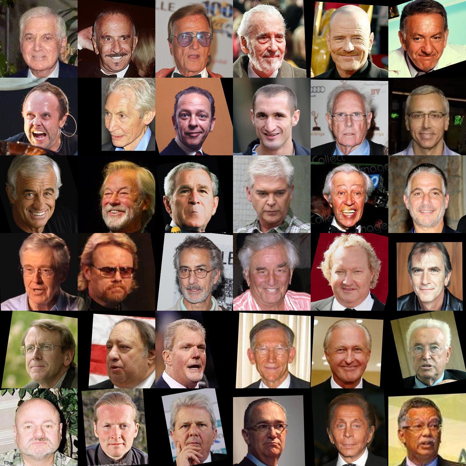
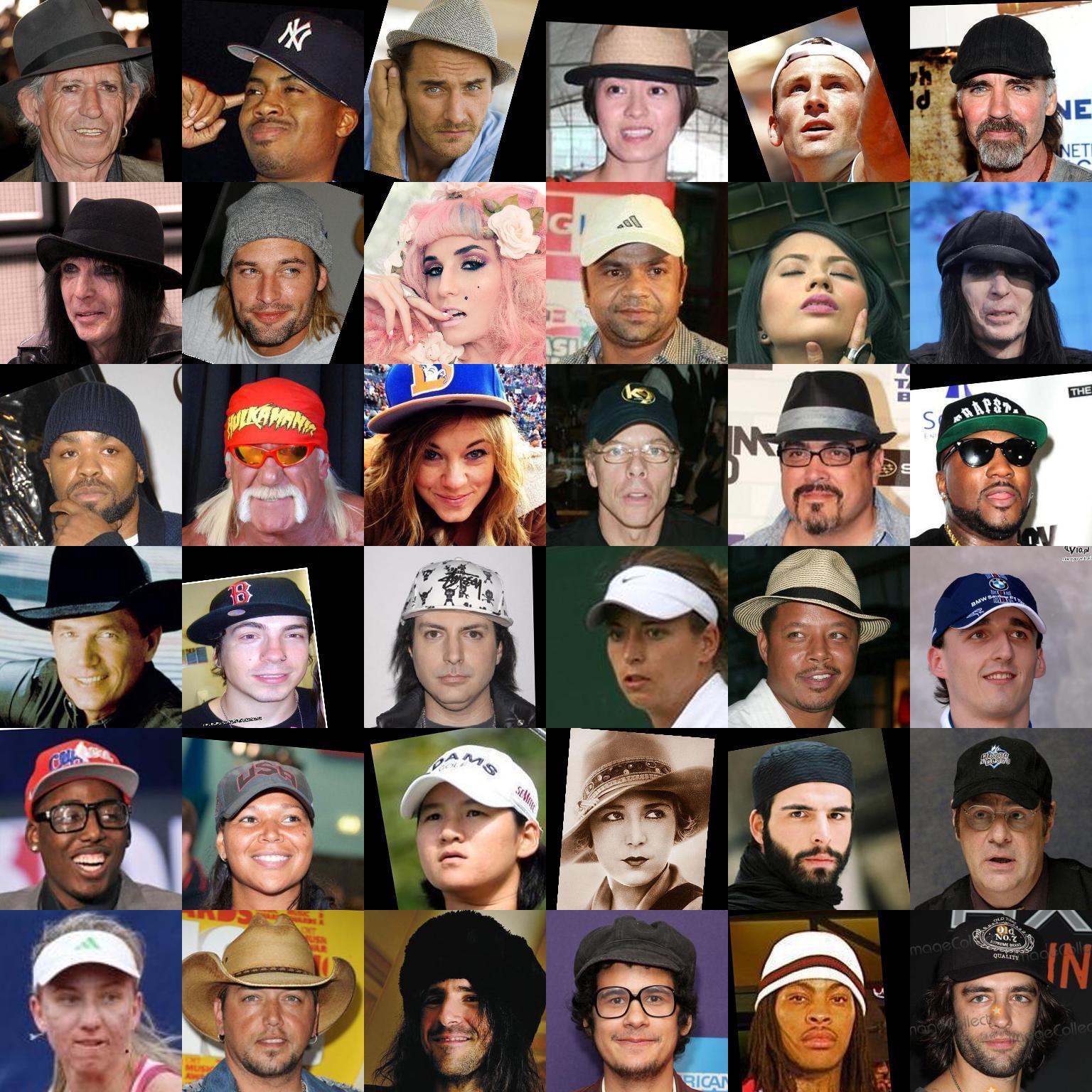
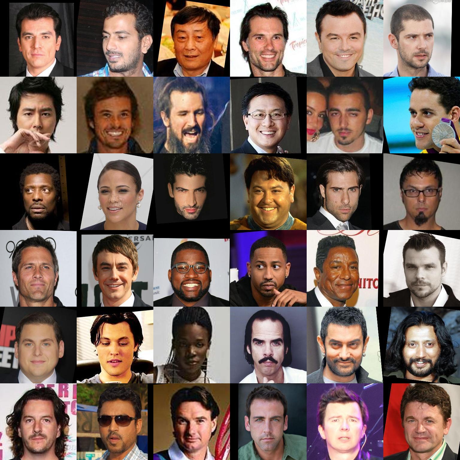
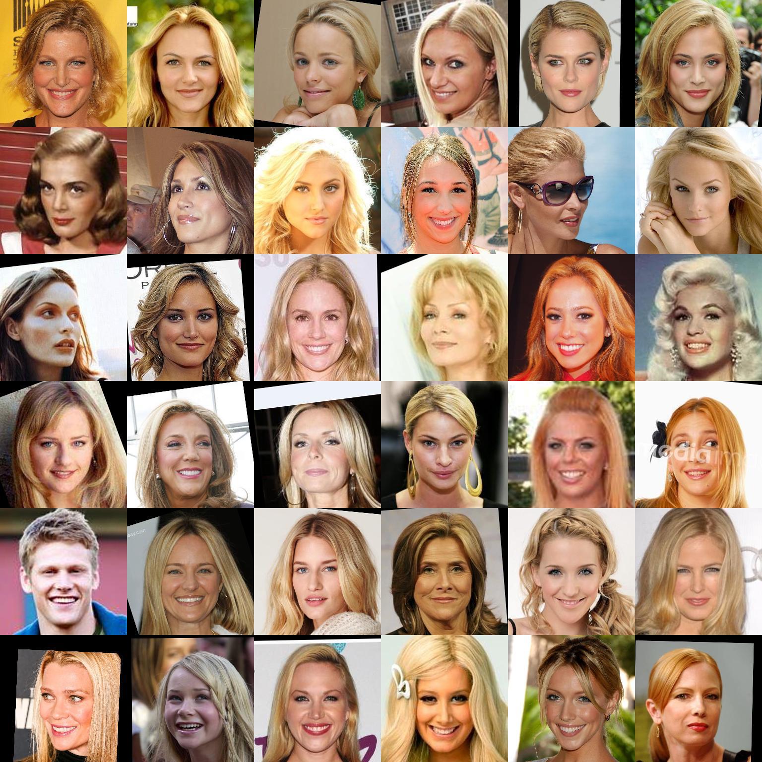
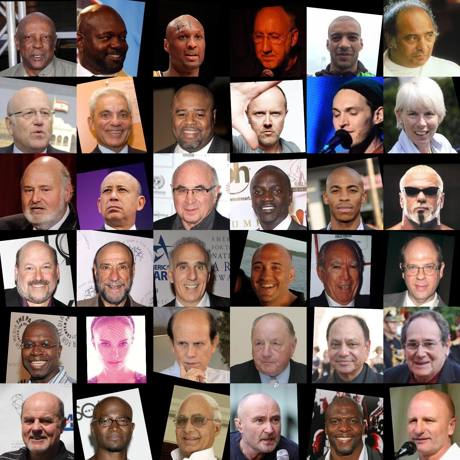
	(a)	(b)	(c)	(d)	(e)
Mouth and Chin
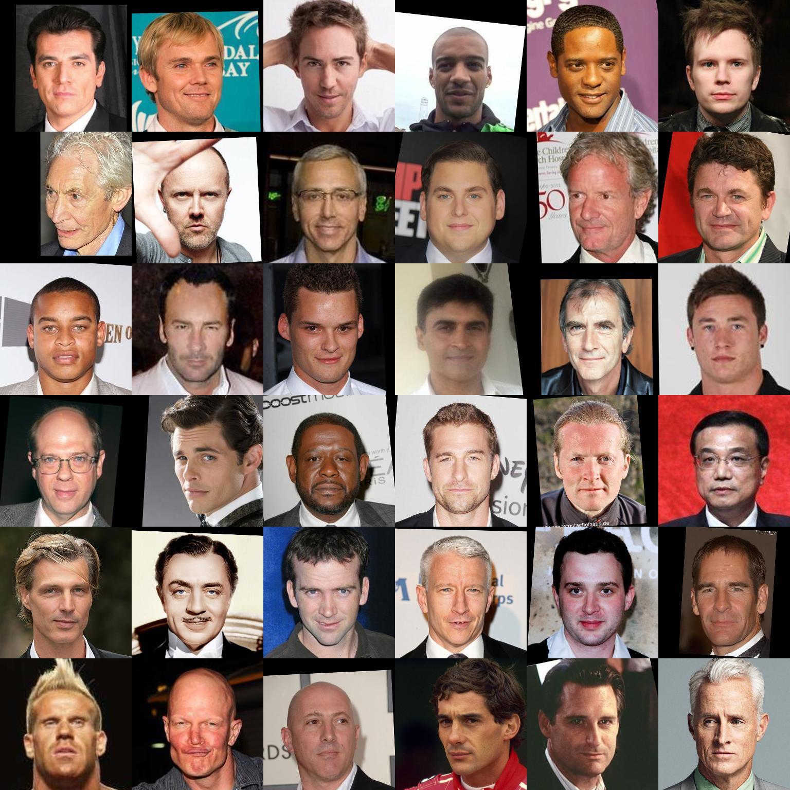
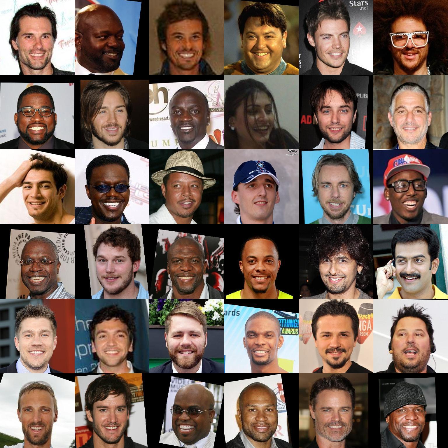
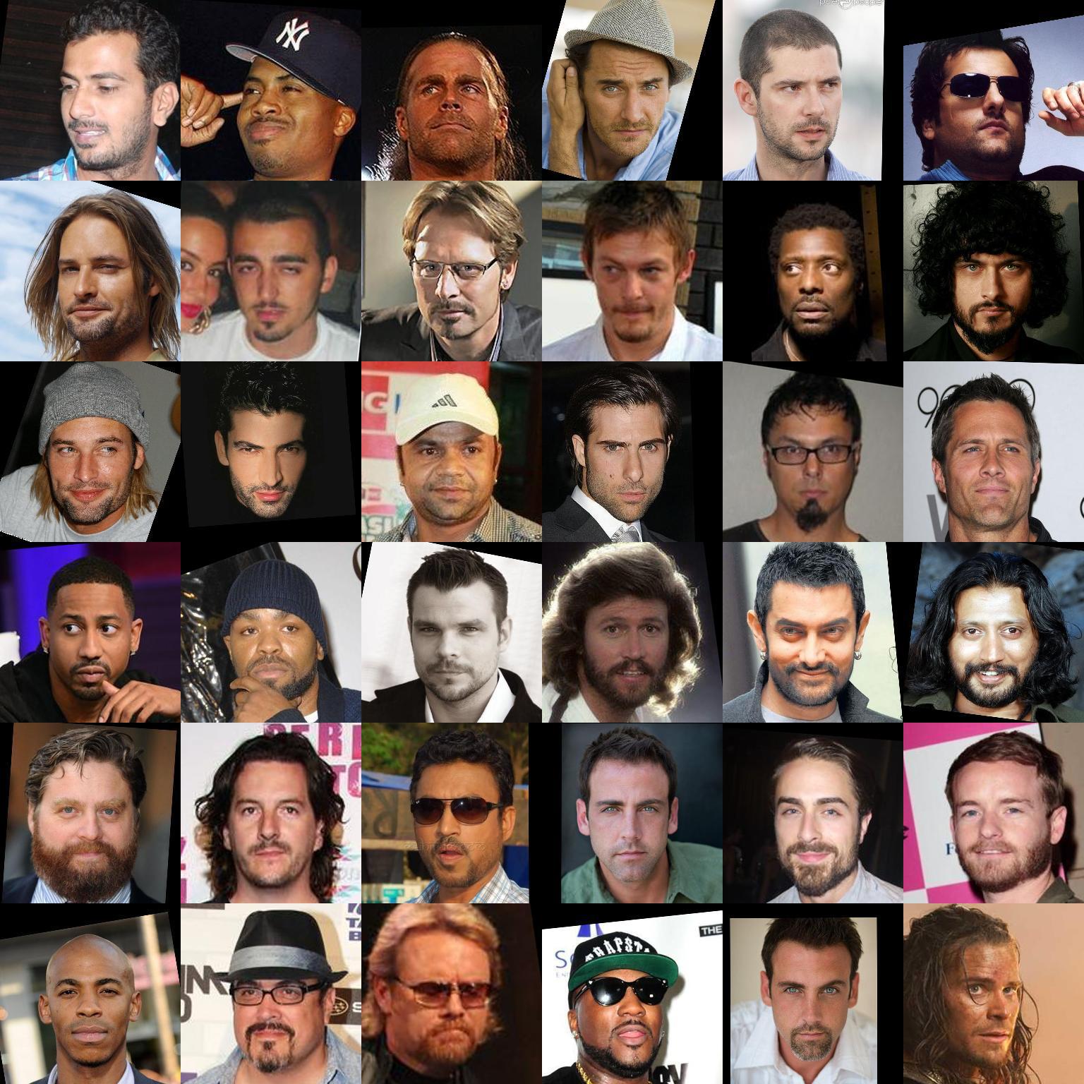
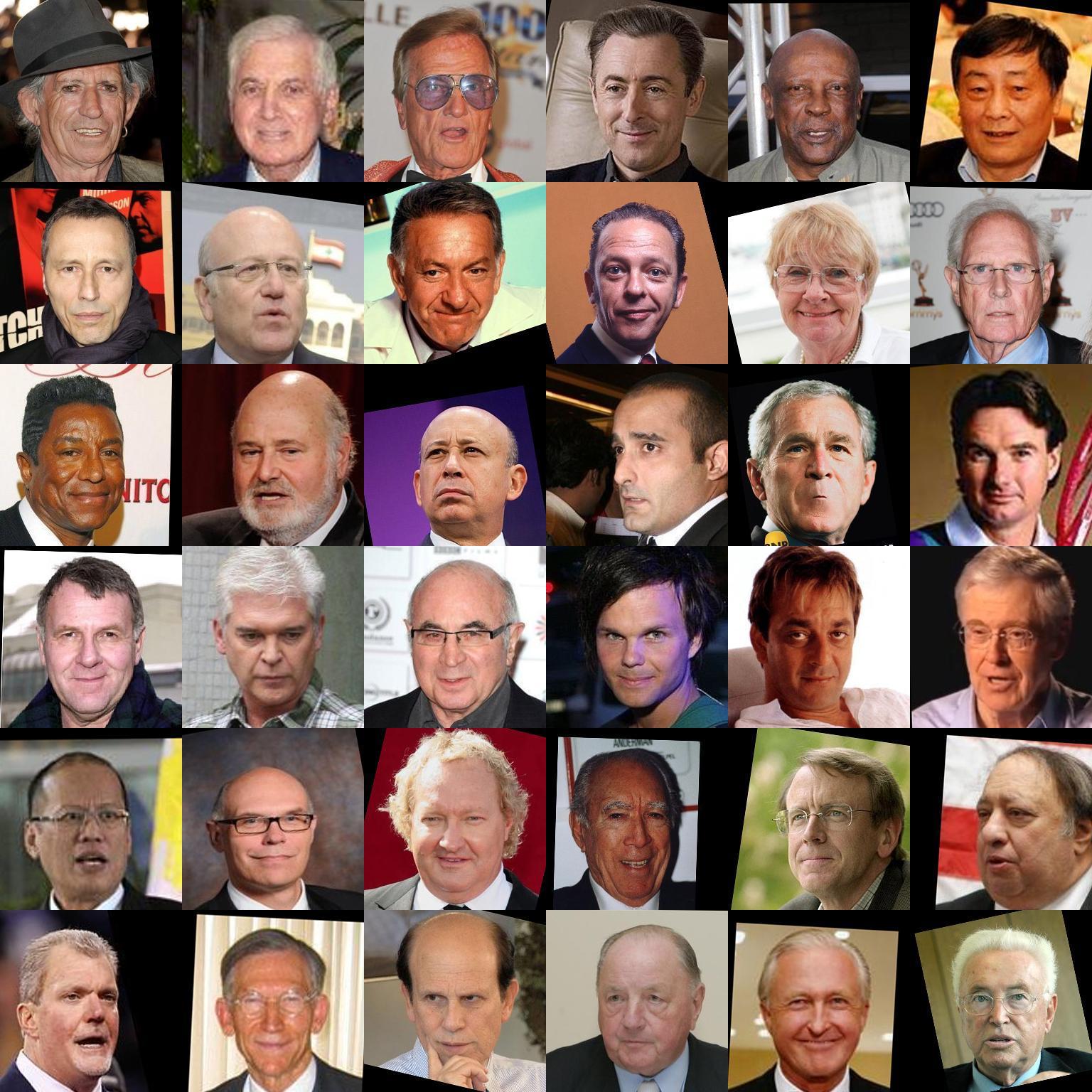
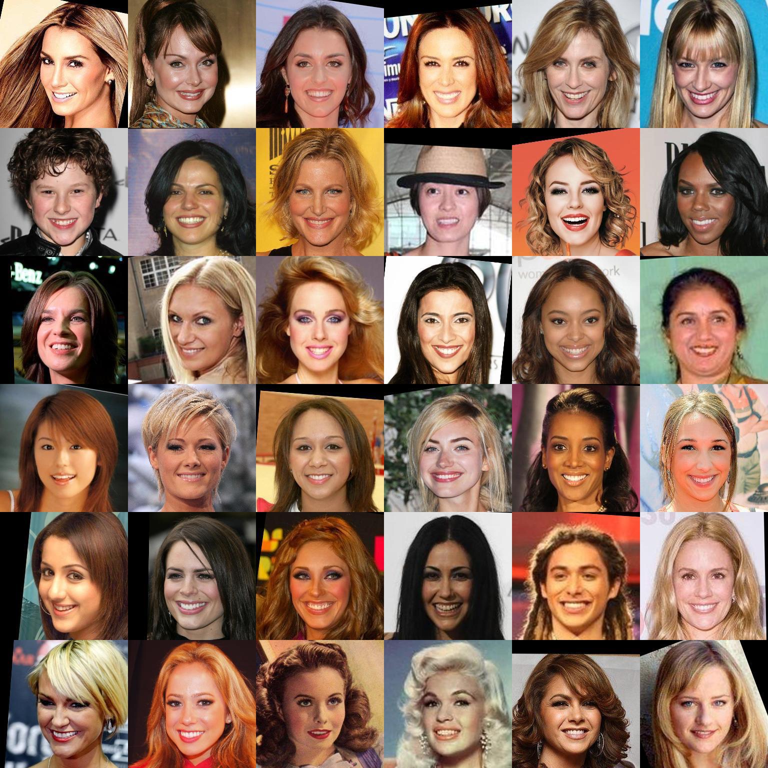
	(a)	(b)	(c)	(d)	(e)

Figure 2: Sample images from subspace clustering of face part embedding in attribute space. Zoom in to see the clusters.

We compare our proposed networks with FaceTracer [19], PANDA [40], and CelebA [21] attribute networks. These models capture a broad spectrum of possible automatic attribute detection models.

FaceTracer [19] attribute classifiers are trained by extracting traditional low-level features like HOG and the color histogram from aligned face parts by incrementally finding the best set of features and training the SVMs on the selected features and parts for attribute detection. The face crops are extracted from the ground truth landmarks.

PANDA employs multiple CNNs for the face parts and concatenates the outputs of the last layer and trains SVMs for each attribute. There are two differences between our network architecture and PANDA networks. First, in PANDA, all of the attributes are associated with all of the parts. Second, in our Multi*-CNNAA networks, the last layer is shared between all of the attributes softmax losses, but in PANDA there are two fully connected layers after the shared fully connected layer for each one. As a result, in our network, the different attributes that are associated with one network lie in the same Euclidean space of the last fully connected layer of the network. We exploit this feature in Section 2.3.

CelebA takes a different approach by pre-training a network with face identities of CelebFaces [33] for both face verification and identification. Then features from multiple overlapping patches of the face and train SVMs for each cropped region and each attribute. To predict an attribute, the scores of SVMs are averaged.

We also follow [20] and train a single task network for each attribute in Binary*-CNNAA on the full face to compare with the most specialized model for each attribute. Table 1 shows the accuracy of each of these methods.

As it can be seen, our Multi*-CNNAA networks give equal or better results than the rest. The MultiWide-CNNAA architectures perform slightly better than the MultiDeep-CNNAA in attribute prediction. However, they are slower and consume more energy as shown in Section 4.

2.3 Attribute discovery

As mentioned in the previous section, our Multi*-CNNAA networks transform the input face regions to a shared Euclidean space for the attributes associated with that part. To further explore this Euclidean space, we perform Sparse Subspace Clustering (SSC) [9] on 10000 points that are selected from the training portion of CelebA dataset. The intuition behind this clustering step is that the data points with the same set of attributes lie on the same side of the learned planes defined by the weights of the last layer of each network. Thus they can be represented as a sparse combination of the neighboring points. SSC uses this fact to find the clusters. Therefore by formulating the clustering problem as

$$\underset{C\in\mathbb{R}^{n\times n}}{\text{minimize}}\ \ \lvert C\rvert_{1}+\lVert D-DC\rVert^{2}_{F}$$ (3)

subject to $$\operatorname{diag}{(C)}=0$$ (4)

where $D\in\mathbb{R}^{d\times n}$ is the data matrix containing $n$ points of dimension $d$ and $C\in\mathbb{R}^{n\times n}$ is the affinity matrix. To enforce the constraint, the authors of [9] find the sparse code of each data point in a dictionary of all the points except the test point. To get the clusters they perform spectral clustering on $C$.

We find 10 clusters per face regions. The clusters corresponding to the “Hair-Forehead” region of the face and the “eyes” region can be seen in Figure 2. As illustrated, the “discovered” attributes overlap with the labels that we had in the training time mostly, however, some attributes are divided into finer categories. For example, the “Hair-Forehead” region cluster (c) contains male images with short hair which was not seen in the labels.

3 Active Authentication

We evaluate the performance of CNNAA for the task of active authentication using two publicly available datasets MOBIO [23] and AA01 [10]. These datasets contain videos of the users interacting with cell phones. We compare the authentication performance of our DCNN attribute detectors and discovered attributes using the baseline Local Binary Patterns [2] and ACA [28, 29] which is the only attribute-based approach for this task on mobile phones. We follow the same protocol as ACA to extract facial parts and video features. So, we average over the extracted attribute outputs for the video frames to get the video descriptors.

We cast the problem of continuous authentication as a face verification problem in which a pair of videos is given to determine whether they contain the same identity or not. To compare the performance of the algorithms, the receiver operating characteristic (ROC) curve is used. Many other measures of performance can be readily extracted from the ROC curve. The ROC curve plots the relationship between false acceptance rates (FARs) and true acceptance rates (TARs) and can be computed from a similarity matrix $S$ between gallery and probe videos. We also report the EER value where False Rejection Rate (FRR) and FAR are equal. EER value gives a good idea of the ROC curve shape, since the value $1-EER$ is where the line $x+y+1=0$ meets the ROC curve. Thus, the better the algorithm, the lower is its EER value.

We give each video frame to the CNNAA networks and predict the attributes with linear SVMs. For the learned attributes, we put the probabilistic output of the SVMs which are trained by LIBSVM [5] as our final attribute feature. Since the attribute outputs of our models are probability values we get the similarity value $s_{i,j}=\langle e_{i},t_{j}\rangle$, where $e_{i}$ is the feature vector for the enrollment video and $t_{i}$ is the test video features.

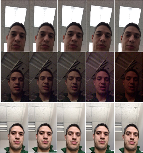
Figure 3: Sample images of the three sessions of the AA01 dataset.

To use the discovered attributes (DiscAttrs) for authentication, we extract the attribute features by a similar approach to Sparse Representation Classification [36]. Each face crop from the video frame is embedded to the attribute space of MultiDeep-CNNAA. It is represented by the dictionary which we used in Section 2.3, so that we know the cluster assignment of its atoms. We normalize all of the dictionary atoms and the embedding. Then we get each feature value by a softmax over the representation contribution of each cluster in the attribute space. To do so, we first solve

$$\underset{f\in\mathbb{R}^{n}}{\text{minimize}} \lvert f\rvert_{1}+\lVert f-Df\rVert_{F}^{2}$$ (5)

to get the sparse representation $f$ of the face crop of that video frame. Then we set the $i$th feature for that face crop to $p(c=i|D)$ which is calculated by

$$p(c=i|D)=\frac{\exp(\lVert D_{:,i}f_{i}\rVert)}{\sum_{k=1}^{10}\exp(\lVert D_{:,k}f_{k}\rVert)}$$ (6)

where $D_{:,i}$ is the dictionary atoms of cluster $i$ and $f_{i}$ are the coefficients corresponding to those atoms. Thus, if $f$ is in the subspace spanned by the points in $D$ that are in cluster $i$, it will have more energy in non-zero values for those atoms. To solve (5) we use the Orthogonal Matching Pursuit [35] algorithm with sparsity 20. The only reason for choosing 20 is that it is less than 32 which is the embedding space dimension. This parameter could be fine tuned further to get better results. Then we concatenate all of these probability values for different face parts to create the final representation. The similarity matrix is then created in the same way as using attributes as features.

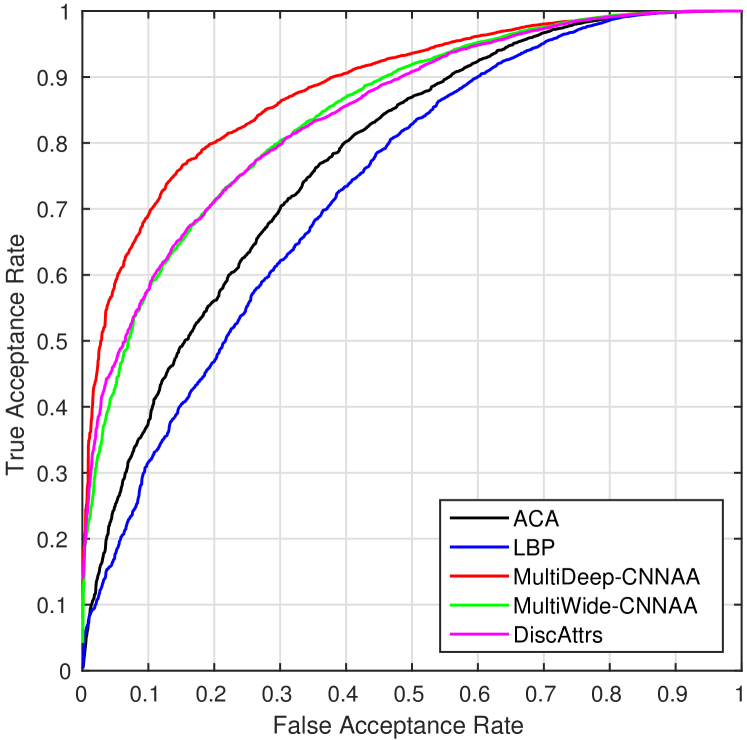
(a) AA01 Altogether

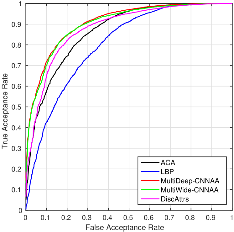
(b) MOBIO mobile

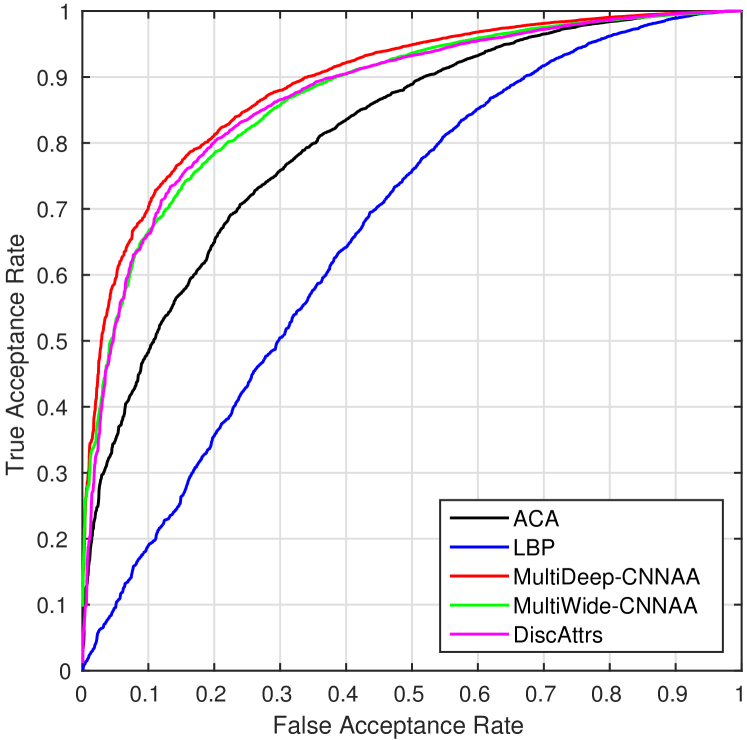
(c) MOBIO cross-sensor

Figure 4: ROC curve of different experiments on AA01 [10] and MOBIO [23] dataset. (a) is the ROC curve of AA01 with all of the sessions together in gallery and probe. (b) is the ROC curve of MOBIO with all of the mobile sessions together with the last session videos as gallery and videos of the rest as probe. (c) is the ROC curve of the cross-device experiment.

$\mathbf{e}\rightarrow\mathbf{t}$	ACA	LBP	MD-CNNAA	MW-CNNAA	DiscAttrs
$1\rightarrow 1$	0.14	0.13	0.11	0.14	0.16
$2\rightarrow 2$	0.19	0.31	0.18	0.22	0.17
$3\rightarrow 3$	0.16	0.20	0.10	0.10	0.13
$1\rightarrow 2,3$	0.38	0.38	0.18	0.25	0.23
$2\rightarrow 1,3$	0.31	0.33	0.26	0.30	0.31
$3\rightarrow 1,2$	0.31	0.38	0.19	0.24	0.25
Altogether	0.30	0.34	0.20	0.25	0.25

Table 4: The EER values for the different experiments on AA01[10] dataset. The sessions numbers are: 1. Office light 2. Low light 3. Natural light. DiscAttrs column contains the EER values using the discovered attributes.

3.1 Results

To plot the ROC curves and evaluate our method, in each dataset, for each person, videos of one session are considered as the enrollment videos and the other videos as the test videos. The similarity matrix is then generated by computing the pairwise similiarity between the enrollment and the test videos. The corresponding ROC curve is plotted for each experiment.

AA01

AA01 is a mobile dataset with 750 videos of 50 subjects. Each subject has three sets of videos with three different lighting conditions. Each user is asked to perform a set of actions on the phone while the front camera is recording the video. The videos are captured by an iPhone 4 camera. The three lighting conditions are: office light, low light, and natural light. The sample images of this dataset in Figure 3 show the three different illuminations in each session. Figure 3 also presents some partial faces in the dataset. Each person has five videos of performing five different tasks on the phone. There is a designated enrollment video for each person. Three different experiments have been conducted on this dataset.

First, the enrollment and the test videos for all of the 50 subjects are taken from the session with the same lighting condition. The EER values of this experiment can be found in the first three rows of Table 4. It can be seen that our MultiDeep-CNNAA has the lowest EER in all cases. This experiment reveals the discriminative power of the features when the surrounding environment is the same. In the second experiment, all of the enrollment videos are taken from one illumination session and the test videos from another. The EER values corresponding to this experiment are depicted in the next three rows of Table 4. The performance drop in our method is $0.08$ while on average while ACA suffers $0.17$ and LBP $0.15$. The reason is that ACA attribute classifiers use low level features that are sensitive to illumination changes, but CNNAA is trained on a large-scale unconstrained dataset containing a lot of variations and thus gives more robust features.

In the last experiment, all of enrollment videos of the three sessions are put in the gallery and all of the test videos in the probe to get the similarity matrix. The ROC curve corresponding to the third general experiment is plotted in Figure 4(a). It can be seen that MultiDeep-CNNAA performs the best and MultiWide-CNNAA and the discovered attributes are tied as second best.

One explanation for the lower performance of MultiWide-CNNAA compared to MultiDeep-CNNAA is that it has many more parameters than MultiDeep-CNNAA according to Table 6 and has overfitted to the celebrity face images distribution.

Figure 5: Sample images of three sessions of the MOBIO dataset. First row images are from different sites, second row has the pairs with the same identities in two different sessions.

MOBIO

MOBIO [23] is a dataset of 152 subjects. The videos are taken in six different universities across Europe. For most subjects, twelve sessions of video are captured. All of the mobile videos are captured with a Nokia N93i. The first session’s videos are also recorded with a 2008 MacBook laptop. We perform two experiments on this dataset. We take the $12$th session videos as our training videos since they are the mostly available videos across the dataset.

In the first experiment, we just consider videos that are taken by the mobile device. We show the EER values for the mobile videos of the subjects within each site, as well as all of the videos together in Table 5. This experiment is similar to the “Altogether” experiment of AA01 dataset since the environment conditions for enrollment videos and test videos can be the same or different. The ROC curve for this experiment is plotted in Figure 4(b).

	ACA	LBP	MD-CNNAA	MW-CNNAA	DiscAttrs
but	0.26	0.36	0.19	0.20	0.23
idiap	0.25	0.35	0.27	0.25	0.24
lia	0.24	0.34	0.17	0.15	0.16
uman	0.27	0.33	0.18	0.20	0.21
unis	0.2	0.27	0.07	0.1	0.1
uoulu	0.18	0.23	0.14	0.14	0.19
Altogether	0.22	0.28	0.17	0.18	0.19
Mobile-PC	0.27	0.38	0.19	0.21	0.2

Table 5: The EER values corresponding to MOBIO dataset experiments.

The second experiment is about the cross sensor authentication, in which you enroll yourself on one device and test on another device. To see how important sensor change can be for low level features, one can look at the performance drop of the LBP features in this experiment and the previous one in Table 5. The decrease is $0.10$ for the LBP features and $0.05$ for ACA which depends on low level features, while CNNAA methods just have a decrease of $0.01$ in EER value. The ROC curve for this experiment is presented in Figure 4(c). Again, this is due to the fact that CNNAA has seen more variations in the large training set. Our method can also handle partial face verification if a partial face detector [22] is available.

4 Mobile performance

Input size	Network	Parameters	Prediction time	Network	Parameters	Prediction time
$128\times 52$	D-UpperHead	275,360	0.15s	W-UpperHead	1,825,664	0.26s
$115\times 41$	D-BothEyes	227,936	0.11s	W-BothEyes	1,447,552	0.19s
$90\times 62$	D-EyesNose	244,704	0.13s	W-EyesNose	1,580,160	0.22s
$40\times 56$	D-Nose	170,400	0.06s	W-Nose	988,032	0.1s
$55\times 82$	D-NoseMouth	232,352	0.10s	W-NoseMouth	1,481,600	0.18s
$65\times 38$	D-Mouth	164,448	0.06s	W-Mouth	939,648	0.11s
$115\times 107$	D-EyesNoseMouth	441,632	0.28s	W-EyesNoseMouth	3,154,304	0.48s
$128\times 45$	D-MouthChin	244,640	0.13s	W-MouthChin	1,579,904	0.23s
$62\times 100$	D-Ear	256,864	0.14s	W-Ear	1,677,952	0.25s
$53\times 39$	D-Eye	162,400	0.06s	W-Eye	923,264	0.08s
Overall	MultiDeep-CNNAA	2.4M	1.22s	MultiWide-CNNAA	15.6M	2.10s
$128\times 128$	BinaryDeep-Full	584,160	0.36s	BinaryWide-Full	4,289,664	0.637s

Table 6: Network size and prediction speed of the networks. The D-* means it has MultiDeep-CNNAA architecture and W-* means it is MultiWide-CNNAA. The Binary*-CNNAA network prediction times are just for one attribute. For all of them together it will be 40 times this value.

There is a trade-off among power consumption, authentication speed, and accuracy of the model for the task of active authentication on mobile devices. The response time is important since we do not want to freeze other running processes and create an unpleasant user experience while authenticating. Power consumption is also important because as frequent demands for charging the battery can be annoying.

To show the effectiveness of our approach, we measure the attribute prediction speed of our networks and the battery consumption on an LG Nexus 5 device. The results are shown in Table 6. This mobile device has a quad-core QUALCOMM Snapdragon 800 clocked at 2.26 GHz and 2 GB of RAM. This specification is considered average compared to the current smartphones. We use the Tensorflow [1] implementation of CNNs on Android devices.

We follow ACA [29] for the performance analysis on the phone. We take one shot with the smartphone camera and feed it to the network 200 times and measure the prediction speed by looking at the average duration per frame. To measure the power usage we use PowerTutor [39] which registers the energy usage per running application and also in total. We do not use the camera continuously because it will bias the response time and power usage of the network. We take the image and the application works in background. The default Android processes are the only other processes that are running besides our application that runs the networks.

According to Table 6 all the attributes are detected in $1.22s$ with MultiDeep-CNNAA running on CPU in the background without blocking other applications. MultiWide-CNNAA takes $2.10s$. The BinaryDeep-CNNAA takes $14.4s$ and BinaryWide-CNNAA $25.5s$.

The MultiDeep-CNNAA architecture consumes $780mW$ power on average and MultiWide-CNNAA drains $1100mW$ of the battery power. The average battery usage of Android when it is not running the CNNAA networks is $600mW$ according to PowerTutor. To see how this affects the battery life, suppose the battery capacity is $C$ Watt-hours (Wh). Then

$$d=\frac{C}{P_{n}+\beta\alpha P_{d}}$$ (7)

where $d$ is the mobile device’s battery life, $P_{n}$ is the power consumption in normal use, $P_{d}$ is the power usage of the attribute detection algorithm, $\beta$ is the fraction of time that the mobile device is being used, $\alpha$ is the authentication ratio constant. $\alpha$ shows how often we want to authenticate the user considering the prediction time of the algorithm, i.e. we authenticate every $\frac{T_{a}}{\alpha}$ where $T_{a}$ is the prediction speed of the model. For instance, if $\alpha=0.5$ we authenticate every $2.44s$ using MultiDeep-CNNAA and every $4.2s$ using MultiWide-CNNAA.

To make the feasibility of CNNAA clearer, suppose we authenticate the user using the MultiDeep-CNNAA architecture on the Nexus 5 device. We choose the MultiDeep-CNNAA since it performs well in the authentication task as discussed in Section 3 and also it has a better runtime and power usage. The Nexus 5 has a $2300mAh$ battery with $3.8V$ voltage, so $C=8.74Wh$. $P_{n}=0.6W$ for the “normal usage” state which is when just Android 5 and the default applications are running. This gives $14.5$ hours battery life. Now if $\alpha=1$ which means we want to authenticate with the highest speed possible and if we are using the phone all the time with $\beta=1$ then the battery life will be reduced to $6.3$ hours in the worst case. In a realistic setting with $\beta=0.2$ and $\alpha=0.5$ it becomes $12.85$ hours which is reasonable. Also, if a GPU implementation of CNNs on Android [30] is used, attribute prediction can happen much faster with less energy consumption.

5 Discussion and future direction

We proposed a feasible multi-task DCNN architecture to extract accurate and describable facial attributes on mobile devices. Each network predicts multi facial attributes from a given face component by mapping it to a shared embedding space. We showed that our attribute prediction performance is comparable to state-of-the art. We explored the embedding space and illustrated that we can extract new attributes by looking at subspace clusters of this space. We also showed that our networks perform attribute-based authentication better than the previously proposed method [28, 29]. Finally, we analyzed the feasibility of our method by performing battery usage and prediction speed experiments on an actual mobile device.

In the future, we plan to jointly train this ensemble of networks for the task of face verification and attribute prediction to get a more discriminative embedding space to gain better authentication performance.

References

- [1] M. Abadi, A. Agarwal, P. Barham, E. Brevdo, Z. Chen, C. Citro, G. S. Corrado, A. Davis, J. Dean, M. Devin, S. Ghemawat, I. Goodfellow, A. Harp, G. Irving, M. Isard, Y. Jia, R. Jozefowicz, L. Kaiser, M. Kudlur, J. Levenberg, D. Mané, R. Monga, S. Moore, D. Murray, C. Olah, M. Schuster, J. Shlens, B. Steiner, I. Sutskever, K. Talwar, P. Tucker, V. Vanhoucke, V. Vasudevan, F. Viégas, O. Vinyals, P. Warden, M. Wattenberg, M. Wicke, Y. Yu, and X. Zheng. TensorFlow: Large-scale machine learning on heterogeneous systems, 2015. Software available from tensorflow.org.
- [2] T. Ahonen, A. Hadid, and M. Pietikainen. Face description with local binary patterns: Application to face recognition. Pattern Analysis and Machine Intelligence, IEEE Transactions on, 28(12):2037–2041, 2006.
- [3] M. Antal and L. Z. Szabó. Biometric authentication based on touchscreen swipe patterns. Procedia Technology, 22:862–869, 2016.
- [4] A. Asthana, S. Zafeiriou, S. Cheng, and M. Pantic. Robust discriminative response map fitting with constrained local models. In Computer Vision and Pattern Recognition (CVPR), 2013 IEEE Conference on, pages 3444–3451. IEEE, 2013.
- [5] C.-C. Chang and C.-J. Lin. Libsvm: a library for support vector machines. ACM Transactions on Intelligent Systems and Technology (TIST), 2(3):27, 2011.
- [6] N. L. Clarke and S. M. Furnell. Authenticating mobile phone users using keystroke analysis. International Journal of Information Security, 6(1):1–14, 2007.
- [7] D. Crouse, H. Han, D. Chandra, B. Barbello, and A. K. Jain. Continuous authentication of mobile user: Fusion of face image and inertial measurement unit data. In International Conference on Biometrics, 2015.
- [8] M. Derawi, C. Nickel, P. Bours, and C. Busch. Unobtrusive user-authentication on mobile phones using biometric gait recognition. In International Conference on Intelligent Information Hiding and Multimedia Signal Processing, pages 306–311, Oct 2010.
- [9] E. Elhamifar and R. Vidal. Sparse subspace clustering. In Computer Vision and Pattern Recognition, 2009. CVPR 2009. IEEE Conference on, pages 2790–2797. IEEE, 2009.
- [10] M. E. Fathy, V. M. Patel, and R. Chellappa. Face-based active authentication on mobile devices. In IEEE International Conference on Acoustics, Speech and Signal Processing, 2015.
- [11] T. Feng, Z. Liu, K.-A. Kwon, W. Shi, B. Carbunar, Y. Jiang, and N. Nguyen. Continuous mobile authentication using touchscreen gestures. In IEEE Conference on Technologies for Homeland Security, pages 451–456, Nov 2012.
- [12] M. Frank, R. Biedert, E. Ma, I. Martinovic, and D. Song. Touchalytics: On the applicability of touchscreen input as a behavioral biometric for continuous authentication. IEEE Transactions on Information Forensics and Security, 8(1):136–148, Jan 2013.
- [13] L. Fridman, S. Weber, R. Greenstadt, and M. Kam. Active authentication on mobile devices via stylometry, gps location, web browsing behavior, and application usage patterns. IEEE Systems Journal, 2015.
- [14] A. Hadid, J. Heikkila, O. Silven, and M. Pietikainen. Face and eye detection for person authentication in mobile phones. In ACM/IEEE International Conference on Distributed Smart Cameras, pages 101–108, Sept 2007.
- [15] N. M. Inc. Nearly one in three consumers who have lost their mobile devices still do not lock them, new survey shows. ”http://www.prnewswire.com/news-releases/nearly-one-in-three-consumers-who-have-lost-their-mobile-devices-still-do-not-lock-them-new-survey-shows-200410151.html”, 2013.
- [16] A. K. Jain, S. C. Dass, and K. Nandakumar. Can soft biometric traits assist user recognition? In Defense and Security, pages 561–572. International Society for Optics and Photonics, 2004.
- [17] D. Kingma and J. Ba. Adam: A method for stochastic optimization. arXiv preprint arXiv:1412.6980, 2014.
- [18] A. Krizhevsky, I. Sutskever, and G. E. Hinton. Imagenet classification with deep convolutional neural networks. In Advances in neural information processing systems, pages 1097–1105, 2012.
- [19] N. Kumar, P. N. Belhumeur, and S. K. Nayar. FaceTracer: A Search Engine for Large Collections of Images with Faces. In European Conference on Computer Vision (ECCV), pages 340–353, Oct 2008.
- [20] G. Levi and T. Hassner. Age and gender classification using convolutional neural networks. In IEEE Conf. on Computer Vision and Pattern Recognition (CVPR) workshops, June 2015.
- [21] Z. Liu, P. Luo, X. Wang, and X. Tang. Deep learning face attributes in the wild. In Proceedings of International Conference on Computer Vision (ICCV), December 2015.
- [22] U. Mahbub, V. M. Patel, D. Chandra, B. Barbello, and R. Chellappa. Partial face detection for continuous authentication. arXiv preprint arXiv:1603.09364, 2016.
- [23] C. McCool, S. Marcel, A. Hadid, M. Pietikainen, P. Matejka, J. Cernocky, N. Poh, J. Kittler, A. Larcher, C. Levy, D. Matrouf, J.-F. Bonastre, P. Tresadern, and T. Cootes. Bi-modal person recognition on a mobile phone: using mobile phone data. In IEEE ICME Workshop on Hot Topics in Mobile Multimedia, July 2012.
- [24] K. Niinuma, U. Park, and A. K. Jain. Soft biometric traits for continuous user authentication. Information Forensics and Security, IEEE Transactions on, 5(4):771–780, 2010.
- [25] O. M. Parkhi, A. Vedaldi, and A. Zisserman. Deep face recognition. In British Machine Vision Conference, 2015.
- [26] L. Prechelt. Automatic early stopping using cross validation: quantifying the criteria. Neural Networks, 11(4):761–767, 1998.
- [27] A. Primo, V. Phoha, R. Kumar, and A. Serwadda. Context-aware active authentication using smartphone accelerometer measurements. In Computer Vision and Pattern Recognition Workshops (CVPRW), 2014 IEEE Conference on, pages 98–105, June 2014.
- [28] P. Samangouei, V. M. Patel, and R. Chellappa. Attribute-based continuous user authentication on mobile devices. In Biometrics Theory, Applications and Systems (BTAS), 2015 IEEE 7th International Conference on, pages 1–8, Sept 2015.
- [29] P. Samangouei, V. M. Patel, and R. Chellappa. Facial attributes for active authentication on mobile devices. Image and Vision Computing, 2016.
- [30] S. Sarkar, V. M. Patel, and R. Chellappa. Deep feature-based face detection on mobile devices. arXiv preprint arXiv:1602.04868, 2016.
- [31] F. Schroff, D. Kalenichenko, and J. Philbin. Facenet: A unified embedding for face recognition and clustering. In Proceedings of the IEEE Conference on Computer Vision and Pattern Recognition, pages 815–823, 2015.
- [32] Y. Sun, Y. Chen, X. Wang, and X. Tang. Deep learning face representation by joint identification-verification. In Advances in Neural Information Processing Systems, pages 1988–1996, 2014.
- [33] Y. Sun, Y. Chen, X. Wang, and X. Tang. Deep learning face representation by joint identification-verification. In Advances in Neural Information Processing Systems, pages 1988–1996, 2014.
- [34] Y. Taigman, M. Yang, M. Ranzato, and L. Wolf. Deepface: Closing the gap to human-level performance in face verification. In Proceedings of the IEEE Conference on Computer Vision and Pattern Recognition, pages 1701–1708, 2014.
- [35] J. A. Tropp and A. C. Gilbert. Signal recovery from random measurements via orthogonal matching pursuit. Information Theory, IEEE Transactions on, 53(12):4655–4666, 2007.
- [36] J. Wright, A. Y. Yang, A. Ganesh, S. S. Sastry, and Y. Ma. Robust face recognition via sparse representation. Pattern Analysis and Machine Intelligence, IEEE Transactions on, 31(2):210–227, 2009.
- [37] H. Zhang, V. M. Patel, and R. Chellappa. Robust multimodal recognition via multitask multivariate low-rank representations. In IEEE International Conference on Automatic Face and Gesture Recognition. IEEE, 2015.
- [38] H. Zhang, V. M. Patel, M. E. Fathy, and R. Chellappa. Touch gesture-based active user authentication using dictionaries. In IEEE Winter conference on Applications of Computer Vision. IEEE, 2015.
- [39] L. Zhang, B. Tiwana, Z. Qian, Z. Wang, R. P. Dick, Z. M. Mao, and L. Yang. Accurate online power estimation and automatic battery behavior based power model generation for smartphones. In Proceedings of the eighth IEEE/ACM/IFIP international conference on Hardware/software codesign and system synthesis, pages 105–114. ACM, 2010.
- [40] N. Zhang, M. Paluri, M. Ranzato, T. Darrell, and L. Bourdev. Panda: Pose aligned networks for deep attribute modeling. In Computer Vision and Pattern Recognition (CVPR), 2014 IEEE Conference on, pages 1637–1644. IEEE, 2014.
- [41] Y. Zhong and Y. Deng. Sensor orientation invariant mobile gait biometrics. In Biometrics (IJCB), 2014 IEEE International Joint Conference on, pages 1–8. IEEE, 2014.