Extrapolation methods and Bethe ansatz for the asymmetric exclusion process

Abstract

The one-dimensional asymmetric simple exclusion process (ASEP), where $N$ hard-core particles hop forward with rate $1$ and backward with rate $q<1$, is considered on a periodic lattice of $L$ site. Using KPZ universality and previous results for the totally asymmetric model $q=0$, precise conjectures are formulated for asymptotics at finite density $\rho=N/L$ of ASEP eigenstates close to the stationary state. The conjectures are checked with high precision using extrapolation methods on finite size Bethe ansatz numerics. For weak asymmetry $1-q\sim 1/\sqrt{L}$, double extrapolation combined with an integer relation algorithm gives an exact expression for the spectral gap up to $10$-th order in the asymmetry.

Keywords: ASEP, extrapolation, Bethe ansatz, asymptotics of determinants

PACS numbers: 02.30.Ik, 47.70.Nd

1 Introduction

The one-dimensional asymmetric simple exclusion process (ASEP) [1, 2] is a Markov process describing hard-core particles moving locally on a lattice, with the exclusion constraint that each site is either empty or contains a single particle. The particles hop of one site in the forward direction with rate $1$ and of one site in the backward direction with rate $q$, $0\leq q<1$, if the destination site is empty. We consider in this paper the model with $N$ particles on a periodic lattice of $L$ sites, in the limit $L,N\to\infty$ with fixed density $\rho=N/L$, $0<\rho<1$.

It is expected that the only influence of the asymmetry parameter $q$ on the large scale behaviour is a rescaling of time by a factor $1-q$ for fixed $q<1$. This was shown for the model defined on the infinite line $\mathbb{Z}$ [3, 4] and for stationary fluctuations in the periodic model [5, 6]. More generally, ASEP belongs at large scale to KPZ [7] universality [8, 9, 10, 11], which also describes fluctuations in some classes of driven diffusive systems, interface growth models and directed polymers in random media. KPZ universality is characterized in one dimension by a dynamical exponent $z=3/2$. For a finite system of $L$ sites, it leads to different behaviours at short time and long time, with a crossover on the relaxation scale $t\sim L^{3/2}$. The short time behaviour corresponds to the model defined on the infinite line, where there is much evidence for KPZ universality [12, 13], and where fluctuations are characterized by Tracy-Widom distributions from random matrix theory. The long time behaviour corresponds to the non-equilibrium steady state, and there is also reasonable evidence for the universality of KPZ fluctuations there, with the Derrida-Lebowitz stationary large deviation function appearing for several models [5, 14, 6, 15, 16, 17].

ASEP is an exactly solvable model. Its generator is the Hamiltonian of a twisted XXZ spin chain with anisotropy $\Delta=(q^{1/2}+q^{-1/2})/2>1$, which is diagonalizable using Bethe ansatz. The study of the large scale behaviour of ASEP requires asymptotics of the eigenvalues and the eigenvectors of the generator. Very explicit formulas were obtained recently [18] for such asymptotics in the totally asymmetric model (TASEP) $q=0$, due to the special structure of the Bethe equations when $\Delta\to\infty$, leading to exact expressions for fluctuations on the relaxation scale. Another approach based on the propagator is also possible [19]. Under the assumption that KPZ universality holds in the crossover between the short and long time limits, the TASEP asymptotics should also be valid for ASEP with $0<q<1$. Precise conjectures are formulated in this paper for the eigenstates. They are checked numerically with high precision using powerful extrapolation methods applied to finite size Bethe ansatz numerics. The extrapolation methods also allow to probe the weakly asymmetric regime $1-q\sim 1/\sqrt{L}$ corresponding to a crossover to equilibrium fluctuations, which we illustrate for the spectral gap.

In section 2, we summarize various finite size Bethe ansatz formulas for the eigenstates of ASEP, with the algebraic formulation of Bethe ansatz recalled in A, and numerical schemes for solving the Bethe equations discussed in B. Conjectures for asymptotics of ASEP eigenstates and their consequences for current fluctuations are stated in section 3. The asymptotics are checked numerically using extrapolation methods in section 4, where the case of the spectral gap for weak asymmetry is also discussed.

2 Bethe ansatz for ASEP

In this section, we summarize known finite size Bethe ansatz formulas for the eigenstates of ASEP. Some of them were already known in the context of ASEP, others are translated from the literature on the XXZ spin chain.

2.1 Master equation

ASEP is a Markov process. The probability $P_{t}(\mathcal{C})$ to observe the system in a configuration $\mathcal{C}$ at time $t$ is given by a master equation. Then

$$|P_{t}\rangle=\rme^{tM}|P_{0}\rangle\;$$ (1)

with $M$ the Markov matrix, $\langle\mathcal{C}|P_{t}\rangle=P_{t}(\mathcal{C})$, and $\langle\mathcal{C}_{0}|P_{0}\rangle$ the initial probabilities at time $0$. We consider the (time-integrated) current $Q_{0}$ between site $L$ and site $1$ up to time $t$, defined as the number of moves of particles from site $L$ to site $1$ minus the number of moves from site $1$ to site $L$. The generating function of $Q_{0}$ can be computed using a deformation $M(\gamma)$ of the Markov matrix, with $\gamma$ a fugacity conjugate to the current and $M(0)=M$. The deformed generator $M(\gamma)$ can be written $M(\gamma)=\sum_{i=1}^{L}M_{i,i+1}(\gamma)$ with local operators $M_{i,i+1}(\gamma)$ acting only on sites $i$ and $i+1$. Their matrix in the local basis $(1_{i}\,1_{i+1},\,1_{i}\,0_{i+1},\,0_{i}\,1_{i+1},\,0_{i}\,0_{i+1})$, with $1$ and $0$ denoting respectively occupied and empty sites, is

$$M_{i,i+1}(\gamma)=\left(\begin{array}[]{cccc}0&0&0&0\\ 0&-1&q\,\rme^{-\gamma}&0\\ 0&\rme^{\gamma}&-q&0\\ 0&0&0&0\end{array}\right)_{\!\!i,i+1}\;.$$ (2)

The generating function of the current is then equal to [18]

$$\langle\rme^{L\gamma Q_{0}}\rangle=\sum_{\mathcal{C}}\langle\mathcal{C}|\rme^{-\gamma S}\rme^{tM(\gamma)}\rme^{\gamma S}|P_{0}\rangle\;.$$ (3)

The operator $S$, diagonal in configuration basis, is defined by $S|\mathcal{C}\rangle=\big{(}\sum_{j=1}^{N}x_{j}\big{)}|\mathcal{C}\rangle$. The $x_{j}$’s, $1\leq x_{j}\leq L$, are the positions of the particles counted from site $1$.

2.2 Bethe ansatz

The matrix $M(\gamma)$ can be diagonalized using Bethe ansatz, see e.g. [5]. Each eigenstate is completely characterized by $N$ complex numbers $y_{j}$, $j=1,\ldots,N$, the Bethe roots, that satisfy a set of $N$ polynomial equations called the Bethe equations:

$$\rme^{L\gamma}\Big{(}\frac{1-y_{j}}{1-qy_{j}}\Big{)}^{L}=-\prod_{k=1}^{N}\frac{y_{j}-qy_{k}}{qy_{j}-y_{k}}\;.$$ (4)

The corresponding eigenvalue of $M(\gamma)$ is equal to

$$E=(1-q)\sum_{j=1}^{N}\Big{(}\frac{1}{1-y_{j}}-\frac{1}{1-qy_{j}}\Big{)}\;,$$ (5)

and the eigenvalue of the translation operator is

$$\rme^{2\rmi\pi p/L}=\rme^{N\gamma}\prod_{j=1}^{N}\frac{1-y_{j}}{1-qy_{j}}\;$$ (6)

with $p\in\mathbb{Z}$ the total momentum.

The right and left eigenvectors of $M(\gamma)$, defined from the algebraic Bethe ansatz in A, can be written explicitly in coordinate form. For a configuration with positions $\mathbf{x}$ ordered as $1\leq x_{1}<\ldots<x_{N}\leq L$, one has

$$\langle\mathbf{x}|\psi\rangle=(1-q)^{N}\rme^{-\frac{N(N+1)}{2}\gamma}\sum_{\sigma\in\mathcal{S}_{N}}\prod_{j=1}^{N}\Bigg{(}\frac{\rme^{\gamma x_{j}}y_{j}}{1-y_{j}}\bigg{(}\frac{1-y_{\sigma(j)}}{1-qy_{\sigma(j)}}\bigg{)}^{x_{j}}\Bigg{)}$$ (7)

$$\hskip 170.71652pt\times\prod_{j=1}^{N}\prod_{k=j+1}^{N}\frac{y_{\sigma(j)}-qy_{\sigma(k)}}{y_{\sigma(j)}-y_{\sigma(k)}}\;$$

$$\langle\psi|\mathbf{x}\rangle=(1-q)^{N}\rme^{-\frac{N(N+1)}{2}\gamma}\sum_{\sigma\in\mathcal{S}_{N}}\prod_{j=1}^{N}\Bigg{(}\frac{\rme^{\gamma(1-x_{j})}}{1-y_{j}}\bigg{(}\frac{1-y_{\sigma(j)}}{1-qy_{\sigma(j)}}\bigg{)}^{1-x_{j}}\Bigg{)}$$ (8)

$$\hskip 170.71652pt\times\prod_{j=1}^{N}\prod_{k=j+1}^{N}\frac{qy_{\sigma(j)}-y_{\sigma(k)}}{y_{\sigma(j)}-y_{\sigma(k)}}\;,$$

with $\mathcal{S}_{N}$ the set of $N!$ permutations of $\{1,2,\ldots,N\}$. Since $M(\gamma)$ is not Hermitian, the left and right eigenstates are different. They verify however $(\prod_{j=1}^{N}y_{j}^{-1})\langle\mathbf{x}|\psi\rangle=\langle\psi|\mathbf{\tilde{x}}\rangle$ with $\mathbf{\tilde{x}}$ related to $\mathbf{x}$ by space reversal, $\tilde{x}_{j}=L+1-x_{N+1-j}$, $j=1,\ldots,N$, since transposing $M(\gamma)$ is the same as reversing space.

Completeness of the Bethe ansatz is the hypothesis that the Bethe equations (4) have exactly $\Omega={L\choose N}$ acceptable solutions such that the corresponding eigenvectors form a complete basis of the space generated by configurations with $N$ particles. Completeness is widely believed to be true based on numerics for small systems, but is difficult to prove rigorously, see however [20, 21, 22] for mathematical results for the exclusion process.

2.3 Scalar product of Bethe eigenstates

The Bethe eigenstates are not normalized. Their scalar product is given by the Gaudin determinant [23, 24]

$$\hskip 42.67912pt\langle\psi|\psi\rangle=(-1)^{N}(1-q)^{N}\rme^{-N^{2}\gamma}\Bigg{(}\prod_{j=1}^{N}y_{j}\Bigg{)}\Bigg{(}\prod_{j=1}^{N}\prod_{k=j+1}^{N}\frac{(y_{j}-qy_{k})(qy_{j}-y_{k})}{(y_{j}-y_{k})^{2}}\Bigg{)}$$

$$\hskip 113.81102pt\times\det\Bigg{(}\partial_{y_{i}}\log\bigg{(}\Big{(}\frac{1-y_{j}}{1-qy_{j}}\Big{)}^{L}\prod_{k=1}^{N}\frac{qy_{j}-y_{k}}{y_{j}-qy_{k}}\bigg{)}\Bigg{)}_{i,j=1,\ldots,N}\;.$$ (9)

The derivative with respect to $y_{i}$ in the determinant has to be computed before setting the $y_{j}$’s equal to a solution of the Bethe equations (4). At $q=0$, the determinant can be calculated explicitly [25], which allows the asymptotic analysis for large $L$, $N$ [26].

The Gaudin determinant is a consequence of the Slavnov determinant [27] for the scalar product between a Bethe eigenstate $\psi_{\mathbf{y}}$ with Bethe roots $y_{j}$ and a Bethe vector $\psi_{\mathbf{w}}$ with arbitrary parameters $w_{j}$ not solution of Bethe equations,

$$\langle\psi_{\mathbf{y}}|\psi_{\mathbf{w}}\rangle=(-1)^{\frac{N(N-1)}{2}}\Big{(}\prod_{j=1}^{N}\prod_{k=1}^{N}(w_{j}-y_{k})\Big{)}$$ (10)

$$\hskip 85.35826pt\times\Big{(}\prod_{j=1}^{N}\prod_{k=j+1}^{N}\frac{1}{(w_{j}-w_{k})(y_{j}-y_{k})}\Big{)}\det\Big{[}\partial_{y_{j}}E(w_{k})\Big{]}_{j,k}\;.$$

The quantity

$$E(w)=\rme^{-N\gamma}\prod_{j=1}^{N}\frac{w-qy_{j}}{w-y_{j}}+\rme^{(L-N)\gamma}\Big{(}\frac{1-w}{1-qw}\Big{)}^{L}\prod_{j=1}^{N}\frac{qw-y_{j}}{w-y_{j}}\;$$ (11)

is the eigenvalue of the transfer matrix $T(w)$, a fundamental object in the algebraic formulation of Bethe ansatz, see A.

2.4 Special configurations

In order to compute the statistics of the current for a given initial condition from the expansion of (3) over eigenstates, the scalar product between the initial configuration and the eigenvectors is needed. Two particularly interesting classes of initial conditions are the flat configurations, where particles are equally spaced, and the step configurations, for which particles occupy consecutive sites. Exact formulas can be written for these two cases, translating previous results for the XXZ spin chain.

Let $\mathcal{F}$ be the flat configuration of a half-filled system $N=L/2$ with particles at positions $x_{j}=2j$, $j=1,\ldots,N$. Then, the XXZ result for the Néel state [28] implies

$$\hskip 28.45274pt\langle\psi|\mathcal{F}\rangle=\frac{(-1)^{\frac{N(N-1)}{2}}\rme^{\frac{N(N+3)\gamma}{2}}}{2^{N(N+1)}}\Bigg{(}\prod_{j=1}^{N}\frac{(1-y_{j})^{L+2}}{y_{j}(1-qy_{j})(1-qy_{j}^{2})}\Bigg{)}$$ (12)

$$\hskip 71.13188pt\times\Bigg{(}\prod_{j=1}^{N}\prod_{k=j+1}^{N}\frac{1}{(y_{j}-y_{k})(1-qy_{j}y_{k})}\Bigg{)}\det\Bigg{(}\Big{(}\frac{1+y_{k}}{1-y_{k}}\Big{)}^{2j}-\Big{(}\frac{1+qy_{k}}{1-qy_{k}}\Big{)}^{2j}\Bigg{)}_{j,k}\;.$$

Let $\mathcal{S}$ be the step configuration with particles at positions $x_{j}=j$, $j=1,\ldots,N$ for arbitrary density $\rho=N/L$. Another result for the XXZ spin chain gives [29]

$$\langle\psi|\mathcal{S}\rangle=\rme^{-\frac{2\rmi\pi pN}{L}}(-1)^{\frac{N(N+1)}{2}}\Bigg{(}\prod_{j=1}^{N}\frac{(1-y_{j})^{N}}{y_{j}}\Bigg{)}\Bigg{(}\prod_{j=1}^{N}\prod_{k=j+1}^{N}\frac{1}{y_{j}-y_{k}}\Bigg{)}$$ (13)

$$\hskip 56.9055pt\times\det\Bigg{(}\frac{1}{(1-qy_{k})^{j}}-\frac{1}{(1-y_{k})^{j}}\Bigg{)}_{j,k}\;.$$

Both (12) and (13) already assume that the $y_{j}$’s are solution of the Bethe equations.

2.5 Sum over configurations

Computing current fluctuations from (3) requires the scalar product between $\sum_{\mathcal{C}}\langle\mathcal{C}|\rme^{-\gamma S}$ and the right eigenstates. The scalar product between left eigenstates and $\sum_{\mathcal{C}}\rme^{\gamma S}|\mathcal{C}\rangle$ is also needed for the stationary initial condition $|P_{0}\rangle\propto\sum_{\mathcal{C}}|\mathcal{C}\rangle$. These scalar products can be computed from the Slavnov determinant (10) similarly to what is done in [30] for TASEP. Indeed, in the limit where all $w_{j}$’s converge to $0$, the Bethe vectors reduce to

$$|\psi_{\mathbf{w}}\rangle\simeq\rme^{-\frac{N(N+1)\gamma}{2}}\Big{(}\prod_{j=1}^{N}\big{(}w_{j}(1-q^{j})\big{)}\Big{)}\rme^{\gamma S}\sum_{\mathcal{C}}|\mathcal{C}\rangle$$ (14)

$$\langle\psi_{\mathbf{w}}|\simeq\rme^{(NL-\frac{N(N-1)}{2})\gamma}\Big{(}\prod_{j=1}^{N}(1-q^{j})\Big{)}\sum_{\mathcal{C}}\langle\mathcal{C}|\rme^{-\gamma S}\;,$$ (15)

and one finds

$$\sum_{\mathcal{C}}\langle\mathcal{C}|\rme^{-\gamma S}|\psi\rangle=\rme^{-\frac{N(N+1)}{2}\gamma}\prod_{j=0}^{N-1}(1-\rme^{-L\gamma}q^{j})$$ (16)

$$\sum_{\mathcal{C}}\langle\psi|\rme^{\gamma S}|\mathcal{C}\rangle=\rme^{-\frac{N(N-1)}{2}\gamma}\Big{(}\prod_{j=1}^{N}y_{j}^{-1}\Big{)}\prod_{j=0}^{N-1}(\rme^{L\gamma}-q^{j})\;.$$ (17)

Furthermore, the mean value and stationary two-point function of the density can be computed by inserting in (3) operators $\eta_{i}$ counting the number of particles ($0$ or $1$) at site $i$. Formulas similar to (16), (17) are then needed with the operator ${\bf 1}_{\{\eta_{1}(\mathcal{C})=0\}}$ inserted. We conjecture

$$\sum_{\mathcal{C}}{\bf 1}_{\{\eta_{1}(\mathcal{C})=0\}}\langle\mathcal{C}|\rme^{-\gamma S}|\psi\rangle=\rme^{-\frac{N(N+1)}{2}\gamma}(\rme^{\frac{2\rmi\pi p}{L}-N\gamma}-\rme^{-L\gamma})\Big{(}\prod_{j=1}^{N-1}(1-\rme^{-L\gamma}q^{j})\Big{)}$$ (18)

$$\sum_{\mathcal{C}}{\bf 1}_{\{\eta_{1}(\mathcal{C})=0\}}\langle\psi|\rme^{\gamma S}|\mathcal{C}\rangle=\rme^{-\frac{N(N-1)}{2}\gamma}\Big{(}\prod_{j=1}^{N}y_{j}^{-1}\Big{)}(\rme^{L\gamma}-\rme^{-\frac{2\rmi\pi p}{L}+N\gamma})\Big{(}\prod_{j=1}^{N-1}(\rme^{L\gamma}-q^{j})\Big{)}\,.$$ (19)

These expressions were first guessed using a computer algebra system for $N=1,2,3$ and $L$ arbitrary, by calculating explicitly the sum over all configurations and replacing each occurrence of $(1-qy_{j})^{L}$ by its expression coming from the Bethe equations (4). The formulas were then confirmed for all $\Omega={L\choose N}$ eigenstates of all systems with $1\leq N<L\leq 9$, $q=0.1$ and a generic value for $\gamma$, by solving numerically the Bethe equations for the eigenstates using the method of B.

3 Asymptotics of ASEP eigenstates

In this section, we consider the first eigenstates of ASEP, whose eigenvalues have a real part scaling as $L^{-3/2}$. We first recall the TASEP results, and then state precise conjectures for ASEP asymptotics guided by KPZ universality.

3.1 First eigenstates of TASEP

Each eigenstate of TASEP, and also of ASEP by continuity, is characterized by a set of $N$ (half-)integers $k_{j}$, $j=1,\ldots,N$, defined in (58). In order to study ASEP on the relaxation scale $t\sim L^{3/2}$, only the eigenstates of $M(\gamma)-(1-q)\rho(1-\rho)L\gamma{\bf 1}$ corresponding to eigenvalues with a real part $\sim L^{-3/2}$ are needed. For TASEP, such eigenstates can be described as quasiparticle-hole excitations over the Fermi sea $k_{j}^{0}=j-(N+1)/2$ representing the stationary state [31, 32], see also [33] for the case with open boundaries. These eigenstates are denoted in the following by the subscript $r$. Each one is described by two finite sets of half integers $\mathbb{P},\mathbb{H}\subset\mathbb{Z}+\frac{1}{2}$, as

$$\{k_{1},\ldots,k_{N}\}=\{k_{1}^{0},\ldots,k_{N}^{0}\}\bigcup\Big{\{}\frac{N}{2}+a,a\in\mathbb{P}^{+}\Big{\}}\bigcup\Big{\{}-\frac{N}{2}+a,a\in\mathbb{P}^{-}\Big{\}}$$

$$\hskip 108.12047pt\;\Big{\backslash}\;\Big{\{}\frac{N}{2}+a,a\in\mathbb{H}^{-}\Big{\}}\;\Big{\backslash}\;\Big{\{}-\frac{N}{2}+a,a\in\mathbb{H}^{+}\Big{\}}\;,$$ (20)

where $\mathbb{P}^{\pm},\mathbb{H}^{\pm}$ represent the positive and negative elements of $\mathbb{P}$ and $\mathbb{H}$. The elements of $\mathbb{P}$ and $\mathbb{H}$ represent respectively momenta of quasiparticle and hole excitations, with total momentum $p_{r}=\sum_{a\in\mathbb{P}}a-\sum_{a\in\mathbb{H}}a$. The cardinals of the sets verify the constraints $|\mathbb{P}^{+}|=|\mathbb{H}^{-}|$ and $|\mathbb{P}^{-}|=|\mathbb{H}^{+}|$. In particular, both $\mathbb{P}$ and $\mathbb{H}$ have the same cardinal $m_{r}=|\mathbb{P}|=|\mathbb{H}|$.

Many TASEP asymptotics of eigenstates are expressed in terms of the function

$$\chi_{r}(v)=\chi_{0}(v)+\sum_{a\in\mathbb{P}}\frac{\omega_{a}^{3}(v)}{3}+\sum_{a\in\mathbb{H}}\frac{\omega_{a}^{3}(v)}{3}\;,$$ (21)

with $\chi_{0}$ defined in terms of the Hurwitz $\zeta$ function as

$$\chi_{0}(v)=\frac{8\pi^{3/2}}{3}\Big{(}\sqrt{-\rmi}\,\zeta\big{(}-\frac{3}{2},\frac{1}{2}+\frac{\rmi v}{2\pi}\big{)}+\sqrt{\rmi}\,\zeta\big{(}-\frac{3}{2},\frac{1}{2}-\frac{\rmi v}{2\pi}\big{)}\Big{)}\;,$$ (22)

and the elementary excitation with momentum $a$

$$\omega_{a}(v)=2\sqrt{\mathrm{sgn}(a)\rmi\pi}\sqrt{|a|+\mathrm{sgn}(a)\frac{\rmi v}{2\pi}}\;.$$ (23)

The function $\chi_{0}$ is analytic for $v$ in $\mathbb{D}=\mathbb{C}\backslash\big{(}\rmi[\pi,\infty)\cup-\rmi[\pi,\infty)\big{)}$. This is also the case for $\omega_{a}$ when $a\in\mathbb{Z}+1/2$, and thus for $\chi_{r}$ for any eigenstate $r$. The function $\chi_{0}$ has an alternative expression as a polylogarithm, $\chi_{0}(v)=-(2\pi)^{-1/2}\mathrm{Li}_{5/2}(-\rme^{v})$ when $\mathrm{Re}\,v<0$ or $\mathrm{Re}\,v>0$, $|\mathrm{Im}\,v|<\pi$.

Asymptotics of eigenstates of $M(\gamma)$ for TASEP with finite rescaled fugacity

$$s=\sqrt{\rho(1-\rho)}L^{3/2}\gamma\;$$ (24)

also involve the quantities $\nu_{r}$ solution of

$$\chi_{r}^{\prime}(\nu_{r})=s\;,$$ (25)

and the function

$$D_{r}(\nu)=\frac{(\frac{\rmi\pi}{2})^{m_{r}^{2}}}{(2\pi)^{m_{r}}}\Big{(}\prod_{a,b\in\mathbb{P}\atop a>b}(a-b)\Big{)}\Big{(}\prod_{a,b\in\mathbb{H}\atop a>b}(a-b)\Big{)}$$ (26)

$$\hskip 42.67912pt\times\exp\Big{(}\lim_{\Lambda\to\infty}-m_{r}^{2}\log\Lambda+\int_{-\Lambda}^{\nu}\rmd v\,\frac{\chi_{r}^{\prime\prime}(v)^{2}}{2}\Big{)}\;.$$

An alternative expression for $D_{r}(\nu)$ as a Cauchy determinant exists [18].

3.2 Numerical conjectures for ASEP eigenstates

From KPZ universality, the eigenvalues of ASEP should be the same as the ones of TASEP in the thermodynamic limit $L\to\infty$ with fixed density $\rho$ and rescaled fugacity $s$, up to a global factor $1-q$: $|E_{r}^{\mathrm{ASEP}}-(1-q)E_{r}^{\mathrm{TASEP}}|\ll\frac{1}{L^{3/2}}$. This was already shown for the gap $r=1$ when $\gamma=0$ [34] and for the stationary state $r=0$ when $\gamma\sim L^{-3/2}$ [6]. For a general eigenstate of ASEP, obtained by continuity after increasing $q$ starting from the TASEP eigenstate with $r=(\mathbb{P},\mathbb{H})$, it leads to

$$\frac{E_{r}}{1-q}\simeq\rho(1-\rho)L\gamma-\frac{2\rmi\pi(1-2\rho)p_{r}}{L}+\sqrt{\rho(1-\rho)}\,\frac{\chi_{r}(\nu_{r})}{L^{3/2}}\;,$$ (27)

with $\chi_{r}$ defined in (21), and $\nu_{r}$ the solution of (25) with rescaled fugacity (24).

From KPZ universality, one also expects that in the thermodynamic limit the Bethe eigenvectors of ASEP are the same as those of TASEP, up to a normalization factor $\lambda(q)$ independent of the eigenstate. From (16) or (18),

$$\lambda(q)=\prod_{j=1}^{\infty}(1-q^{j})=(q;q)_{\infty}\;.$$ (28)

Then (17) and (19) suggest that the asymptotics of the product of the $y_{j}$’s is independent of $q$. From [32], $\prod_{j=1}^{N}y_{j}\simeq\rme^{L[\rho\log\rho+(1-\rho)\log(1-\rho)]}\,\rme^{\nu_{r}}$ and one finds

$$\sum_{\mathcal{C}}\langle\mathcal{C}|\rme^{-\gamma S}|\psi\rangle\simeq\lambda(q)\,\rme^{-\frac{\rho^{2}s\sqrt{L}}{2\sqrt{\rho(1-\rho)}}}\frac{s}{\sqrt{\rho(1-\rho)}\sqrt{L}}$$ (29)

$$\frac{1}{\Omega}\sum_{\mathcal{C}}\langle\psi|\rme^{\gamma S}|\mathcal{C}\rangle\simeq\lambda(q)\,\rme^{\frac{\rho(2-\rho)s\sqrt{L}}{2\sqrt{\rho(1-\rho)}}}\sqrt{2\pi}\,s\,\rme^{-\nu_{r}}$$ (30)

$$\sum_{\mathcal{C}}{\bf 1}_{\{\eta_{1}(\mathcal{C})=0\}}\langle\mathcal{C}|\psi\rangle_{\gamma=0}\simeq\lambda(q)\,\frac{2\rmi\pi p_{r}}{L}$$ (31)

$$\frac{1}{\Omega}\sum_{\mathcal{C}}{\bf 1}_{\{\eta_{1}(\mathcal{C})=0\}}\langle\psi|\mathcal{C}\rangle_{\gamma=0}\simeq\lambda(q)\,\frac{2\rmi\pi p_{r}\sqrt{2\pi}\sqrt{\rho(1-\rho)}\,\rme^{-\nu_{r}}}{\sqrt{L}}\;.$$ (32)

TASEP results also lead to a conjecture for the asymptotics of the norm (2.3) of Bethe eigenstates:

$$\langle\psi_{r}|\psi_{r}\rangle\simeq\lambda(q)^{2}\frac{\rme^{\sqrt{\rho(1-\rho)}\,s\,\sqrt{L}}}{\sqrt{\rho(1-\rho)}\sqrt{L}}\,\frac{\chi_{r}^{\prime\prime}(\nu_{r})}{D_{r}(\nu_{r})^{2}}\;.$$ (33)

Finally, TASEP asymptotics for the components of eigenstates corresponding to a flat configuration (at half-filling $\rho=1/2$) and to a step configuration (at arbitrary filling $\rho$ with sites $1$ through $N$ occupied) lead to

$$\langle\psi_{r}|\mathcal{F}\rangle\simeq{\bf 1}_{\{\mathbb{P}=\mathbb{H}\}}\lambda(q)\rme^{s\sqrt{L}/4}\frac{\rmi^{m_{r}}\rme^{-\nu_{r}/4}}{(1+\rme^{-\nu_{r}})^{1/4}D_{r}}\;$$ (34)

and

$$\langle\psi_{r}|\mathcal{S}\rangle\simeq\lambda(q)\rme^{-2\rmi\pi p_{r}\rho}\;.$$ (35)

3.3 Current fluctuations

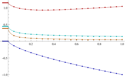
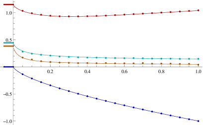
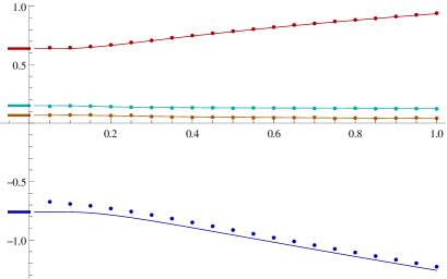
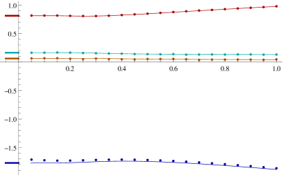
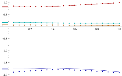
Figure 1: First cumulants of the current $\langle(-\xi_{\tau}/\tau^{1/3})^{k}\rangle_{c}$ plotted as a function of the rescaled time $\tau$, for TASEP (left) and ASEP at $q=0.5$ (right), with stationary initial condition (top row), flat initial condition (middle row) and step initial condition at position $x=0$ (bottom row). In all the plots, the cumulants correspond from top to bottom to $k=2,3,4,1$. The solid lines, computed from (38)-(40), are independent of the asymmetry $q$. The marks on the left are the respective Tracy-Widom values for the cumulants. The dots are results of simulations with $N=1024$ particles on $L=2048$ sites averaged over $5\times 10^{5}$ independent realizations.

The previous asymptotics lead to exact expressions for the current fluctuations in the large $L$ limit with fixed rescaled time

$$\tau=\frac{(1-q)t}{2L^{3/2}}\;$$ (36)

and fixed density of particles $\rho=N/L$. In order to avoid the need of a moving reference frame, required by the typical velocity $1-2\rho$ of density fluctuations, we consider only the half-filled case $\rho=1/2$.

We define the current fluctuations as

$$\xi_{\tau}=\frac{Q_{i}-(1-q)t/4-\mathcal{R}L}{\sqrt{L}/2}\;.$$ (37)

The term $\mathcal{R}$ can be understood from Burgers’ hydrodynamic evolution in the time scale $t\sim L$ [35]. It is equal to $\mathcal{R}=0$ for flat and stationary initial condition and $\mathcal{R}=-|x|/2$ for step initial condition with the current $Q_{i}$ counted at site $i=(x+1/2)L$, $-1/2<x<1/2$.

Expanding (3) over eigenstates and gathering all the asymptotics, one finds for the generating function of current fluctuations

$$\langle\rme^{s\xi_{\tau}}\rangle_{\mathrm{stat}}=\sqrt{2\pi}s^{2}\sum_{r}\frac{D_{r}^{2}(\nu_{r})\,\rme^{\tau\chi_{r}(\nu_{r})}}{\rme^{\nu_{r}}\chi_{r}^{\prime\prime}(\nu_{r})}$$ (38)

$$\langle\rme^{s\xi_{\tau}}\rangle_{\mathrm{flat}}=s\sum_{r}{\bf 1}_{\{\mathbb{P}=\mathbb{H}\}}\frac{\rmi^{m_{r}}D_{r}(\nu_{r})\,\rme^{\tau\chi_{r}(\nu_{r})}}{\rme^{\nu_{r}/4}(1+\rme^{-\nu_{r}})^{1/4}\chi_{r}^{\prime\prime}(\nu_{r})}$$ (39)

$$\langle\rme^{s\xi_{\tau}}\rangle_{\mathrm{step}}=s\sum_{r}\rme^{2\rmi\pi p_{r}x}\,\frac{D_{r}^{2}(\nu_{r})\,\rme^{\tau\chi_{r}(\nu_{r})}}{\chi_{r}^{\prime\prime}(\nu_{r})}\;.$$ (40)

The first cumulants of $\xi_{\tau}$ corresponding to (38)-(40) are plotted in figure 1 along with results from simulations of TASEP and ASEP with $q=1/2$. The agreement is excellent for TASEP, except for the mean value in the step case due to $1/\sqrt{L}$ finite size corrections instead of $1/L$ for all the other cumulants. The agreement is also good for ASEP, except for the mean value with flat and step initial condition.

The functions $\chi_{r}$, $D_{r}$ and the quantities $\nu_{r}$ are defined in section 3.1. At long time (38)-(40) imply that the large deviation function of $\xi_{\tau}$ is the Derrida-Lebowitz function, while at short time numerical evaluations of (38)-(40) indicate that the statistics of $\tau^{-1/3}\xi_{\tau}$ is described by a Tracy-Widom distribution, in agreement with the results on the infinite line [18].

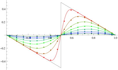
Figure 2: Average density of particles $2\tau\langle\sigma(x,\tau)\rangle$ with step initial condition, plotted for TASEP (left) and ASEP at $q=0.5$ (right) as a function of the position $x$, for times $\tau=0.05,0.1,\ldots,0.4$ from largest to smallest amplitude. The shock obtained at short time is represented in grey. The solid lines, computed from (41), are independent of the asymmetry $q$. The dots are results of simulations with $N=1024$ particles on $L=2048$ sites averaged over $5\times 10^{5}$ independent realizations and $128$ consecutive sites.

The asymptotics of eigenstates also give the mean value and stationary two-point function of the density by setting $\gamma=0$ in (3). By translation invariance, $\langle\eta_{i}\rangle_{\mathrm{stat}}=\langle\eta_{i}\rangle_{\mathrm{flat}}=1/2$. For step initial condition with sites $1$ through $N$ occupied, the density fluctuations $\sigma(x,\tau)=2\sqrt{L}(\eta_{i}-\mbox{\small$\frac{1}{2}$})$ at site $i=(\rho+x)L$ are equal on average to

$$\langle\sigma(x,\tau)\rangle_{\mathrm{step}}=-2\rmi\pi\sum_{r>0}\rme^{2\rmi\pi p_{r}x}\,\frac{p_{r}D_{r}^{2}(\nu_{r})\,\rme^{\tau\chi_{r}(\nu_{r})}}{\chi_{r}^{\prime\prime}(\nu_{r})}\;.$$ (41)

The sum is over all eigenstates $r=(\mathbb{P},\mathbb{H})$ except the stationary eigenstate. The exact expression (41), plotted in figure 2, agrees very well with simulations of TASEP and ASEP.

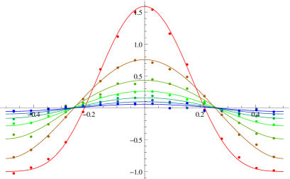
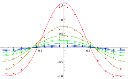
Figure 3: Stationary two-point function of the density of particles $\langle\sigma(0,0)\sigma(x,\tau)\rangle$, plotted for TASEP (left) and ASEP at $q=0.5$ (right) as a function of the position $x$, for times $\tau=0.04,0.08,\ldots,0.28$ from largest to smallest amplitude. The solid lines, computed from (42), are independent of the asymmetry $q$. The dots are results of simulations with $N=256$ particles on $L=512$ sites averaged over $10^{7}$ independent realizations and $32$ consecutive sites.

Similarly, one finds for the stationary two-point function of the density

$$\langle\sigma(0,0)\sigma(x,\tau)\rangle_{\mathrm{stat}}=-(2\pi)^{5/2}\sum_{r>0}\rme^{2\rmi\pi p_{r}x}\,\frac{p_{r}^{2}D_{r}^{2}(\nu_{r})\,\rme^{\tau\chi_{r}(\nu_{r})}}{\rme^{\nu_{r}}\chi_{r}^{\prime\prime}(\nu_{r})}\;.$$ (42)

The stationary two-point function is plotted in figure 3. The agreement with simulations is good, although noticeably worse than for the one-point function due to the smaller system size studied, which was imposed by the much larger number of realizations needed in order to compute accurately the average.

The expressions (38)-(42) are identical to the ones obtained for TASEP in [18]. They look quite similar to discretized functional integrals with the action $\int_{-\infty}^{\nu}\rmd v(\varphi^{\prime}(v)^{2}+\tau\varphi(v))$ of a scalar field in a linear potential. The kinetic part of the action is hidden in $D_{r}^{2}(\nu)$. The discrete realizations $\varphi_{r}$ of the field $\varphi$ are related to the functions $\chi_{r}$ by $\varphi_{r}(v)=\chi_{r}^{\prime}(v)$. Since the value of $\varphi_{r}$ at the upper limit of the integral in the action is equal to $\varphi_{r}(\nu_{r})=s$, one can identify $\varphi_{r}$ as a field conjugate to the current.

4 Extrapolation methods for asymptotics of eigenstates

Exact calculations for TASEP [32, 26] indicate that quantities such as eigenvalues, normalization of Bethe states, and components of Bethe states for simple configurations have a clean asymptotic expansion with exponent $\theta=1/2$

$$\sum_{k=0}^{\infty}a_{k}z^{\theta k}\;$$ (43)

in the variable $z=1/L$. Assuming that the same is true for ASEP, which is supported by the exact calculation [34] of the gap, powerful extrapolation methods can be used to extract numerical evaluations with high accuracy of large $L$ asymptotics from the knowledge of a few finite size values. We believe that extrapolation methods should also be very successful in many other integrable models, due to the the availability of finite size expressions that can be evaluated numerically with high precision for moderately large systems combined with the existence of clean asymptotic expansions (see e.g. [36] for an example in the XXZ spin chain, where expansions with $\theta=1$ are found).

4.1 Richardson extrapolation

Expansions of the form (43) allow an extremely precise evaluation of the leading term $a_{0}$ from the knowledge of a few values $f(z_{1})$, …, $f(z_{n})$ with $0<z_{1}<\ldots<z_{n}$, by removing step by step the contributions of $a_{1}$, $a_{2}$, …, $a_{n-1}$. Starting from the values $f_{m}^{1}=f(z_{m})$, $m=1,\ldots,n$, one builds the triangle

$$\begin{array}[]{lllll}f_{1}^{1}&f_{2}^{1}&\ldots&f_{n-1}^{1}&f_{n}^{1}\\ f_{1}^{2}&f_{2}^{2}&\ldots&f_{n-1}^{2}&\\ \ldots&\ldots&\ldots&&\\ f_{1}^{n-1}&f_{2}^{n-1}&&&\\ f_{1}^{n}&&&&\end{array}$$ (44)

by some iteration procedure, defining $f_{m}^{p}$ in terms of some $f_{j}^{k}$ with $(j,k)$ close to $(m,p)$ and $k<p$. The extrapolated value of $a_{0}$ is then $f_{1}^{n}$, and a possible estimation for the order of magnitude of the error is $|f_{1}^{n}-f_{1}^{n-1}|+|f_{1}^{n}-f_{2}^{n-1}|+|f_{1}^{n-1}-f_{2}^{n-1}|$.

This procedure is called Richardson extrapolation. Several versions exist depending on the precise choice of the iteration. The Aitken-Neville step

$$f_{m}^{p}=f_{m+1}^{p-1}+\frac{f_{m+1}^{p-1}-f_{m}^{p-1}}{\big{(}\frac{z_{m+1}}{z_{m+p+1}}\big{)}^{\theta}-1}$$ (45)

corresponds to polynomial extrapolation: it leads to $f_{1}^{n}=P(0)$ with $P$ the unique interpolating polynomial of degree $n-1$ such that $P(z_{j})=f(z_{j})$, $j=1,\ldots,n$. The Bulirsch-Stoer method [37], which we use in this paper, has

$$f_{m}^{p}=f_{m+1}^{p-1}+\frac{f_{m+1}^{p-1}-f_{m}^{p-1}}{\big{(}\frac{z_{m+1}}{z_{m+p+1}}\big{)}^{\theta}\Big{(}1-\frac{f_{m+1}^{p-1}-f_{m}^{p-1}}{f_{m+1}^{p-1}-f_{m+1}^{p-2}}\Big{)}-1}$$ (46)

with $f_{m}^{0}=0$. The iteration corresponds to rational extrapolation: it leads to $f_{1}^{n}=R(0)$ where $R$ is the unique interpolating rational function with numerator and denominator of respective degrees $\lfloor(n-1)/2\rfloor$ and $\lfloor n/2\rfloor$ such that $R(z_{j})=f(z_{j})$, $j=1,\ldots,n$. Rational extrapolation gives usually better results, especially when $f$ has singularities close to $0$.

Both iteration procedures require for large $n$ the knowledge of the $f(z_{j})$ with high precision. Typically, one needs better precision than the standard $16$ digits double precision in order for the result of the extrapolation to improve when increasing $n$ to values larger than $10$ or $15$.

4.2 Application to asymptotics of ASEP eigenstates

$L$	finite size	extrapolation
$10$	$1.26682+0.65827\rmi$	$1.+0.\rmi$
$20$	$1.26803+0.64323\rmi$	$1.3+0.6\rmi$
$30$	$1.26771+0.63903\rmi$	$1.3+0.6\rmi$
$40$	$1.26709+0.63737\rmi$	$1.2602+0.6370\rmi$
$50$	$1.26648+0.63661\rmi$	$1.26017+0.63698\rmi$
$60$	$1.26593+0.63622\rmi$	$1.260174+0.636979\rmi$
$70$	$1.26546+0.63601\rmi$	$1.2601739+0.6369793\rmi$
$80$	$1.26506+0.63590\rmi$	$1.26017394+0.63697930\rmi$
$90$	$1.26471+0.63585\rmi$	$1.2601739429+0.6369792988\rmi$
$100$	$1.26440+0.63582\rmi$	$1.26017394293+0.63697929878\rmi$
$110$	$1.26414+0.63582\rmi$	$1.260173942929+0.636979298781\rmi$
$120$	$1.26390+0.63583\rmi$	$1.260173942929+0.636979298781\rmi$
$130$	$1.26370+0.63585\rmi$	$1.260173942929154+0.636979298780668\rmi$
$140$	$1.26351+0.63587\rmi$	$1.2601739429291542+0.6369792987806681\rmi$
$150$	$1.26334+0.63589\rmi$	$1.26017394292915417+0.63697929878066807\rmi$
$160$	$1.26319+0.63591\rmi$	$1.2601739429291541672+0.6369792987806680721\rmi$
$170$	$1.26306+0.63594\rmi$	$1.26017394292915416715+0.63697929878066807205\rmi$
$180$	$1.26293+0.63596\rmi$	$1.260173942929154167146+0.636979298780668072053\rmi$
$190$	$1.26282+0.63599\rmi$	$1.2601739429291541671458+0.6369792987806680720532\rmi$

Table 1: Extrapolation for the scalar product of the stationary eigenstate $\sqrt{L}\,\rme^{-s\sqrt{L}/2}\langle\psi_{0}|\psi_{0}\rangle$ at density $\rho=1/2$, asymmetry $q=0.1$ and rescaled fugacity $s=0.2+\rmi$. The second column corresponds to finite size values. The element at a given row $L$ of the last column is the result of rational extrapolation applied to all finite size values with even system sizes $\leq L$ computed with $1000$ digits precision. A numerical evaluation of (33) gives $\sqrt{L}\,\rme^{-s\sqrt{L}/2}\langle\psi_{0}|\psi_{0}\rangle\approx 1.26017394292915416714584555428+0.6369792987806680720531597991129\rmi$.

We used the rational extrapolation method in order to check the conjectures of section 3 for the asymptotics of ASEP eigenstates. All the computations were done for the generic value of the fugacity $s=0.2+\rmi$.

Numerics for finite systems with $\approx 1000$ digits precision were obtained from the resolution of the Bethe equations using the procedure detailed in B. We used the variant with Newton’s method, which seemed generally faster for our computations, especially for larger systems. This might however be due to our particular implementation, and more advanced methods to solve the system of differential equations in the other variant discussed in B might be faster, in conjunction with Newton’s method in the end to get arbitrary high accuracy.

The finite size calculations were performed at density $\rho=1/2$, $\rho=1/3$ and $\rho=1/4$ with asymmetry $q=0.1$ (respectively $q=0.5$), for all $18$ (resp. $8$) eigenstates $r=(\mathbb{P},\mathbb{H})$ with $M=\sum_{a\in\mathbb{P}}|a|+\sum_{a\in\mathbb{H}}|a|\leq 3$ (resp. $M\leq 2$). The system sizes considered were $L=\rho^{-1}(M+1),\ldots,L_{\mathrm{max}}-\rho^{-1},L_{\mathrm{max}}$ with $L_{\mathrm{max}}$ equal for density $\rho=1/2,\,1/3,\,1/4$ to $L_{\mathrm{max}}=300,390,520$ (resp. $L_{\mathrm{max}}=260,390,520$).

The asymptotics (27) for the eigenvalues was checked by subtracting from the finite size values the first two terms of the asymptotics and multiplying everything by $L^{3/2}$ before using the extrapolation method. The asymptotics (29)-(35) were checked by computing the ratio between the finite size values and the divergent factors of the asymptotics before using the extrapolation method. The finite size values are computed for all system sizes up to the maximal system size considered. The result of the extrapolation method truncated at the estimation of the error is then compared with the conjectured asymptotics. A perfect match was found within the estimated error of the extrapolation method, which corresponds to at least $22$ digits precision in all cases with $q=0.1$ and to at least $8$ digits precision in all cases with $q=0.5$.

4.3 Application to the spectral gap of WASEP: double extrapolation

The extrapolation method can also be useful in cases where asymptotics are not known. We illustrate this here in the weakly asymmetric regime (WASEP), where

$$1-q=\frac{\mu}{\sqrt{L}}\;$$ (47)

with fixed $\mu$. This regime corresponds to the crossover between KPZ and equilibrium fluctuations, for which few analytical results have been obtained so far with periodic boundary conditions. We focus on half-filled case $\rho=1/2$ with fugacity $\gamma=0$ and consider the spectral gap $E_{1}$, equal to the non-zero eigenvalue with largest real part. One expects

$$E_{1}\simeq\frac{e_{1}(\mu)}{L^{2}}\;.$$ (48)

The function $e_{1}$ is plotted in figure (4). For the symmetric exclusion process $q=1$, $E_{1}\simeq-4\pi^{2}/L^{2}$ [31], thus $e_{1}(0)=-4\pi^{2}$. Extrapolation of finite size numerics with $L=2,4,\ldots,70$ for $\mu=1,0.1,0.01,0.001$ strongly indicates $e_{1}(\mu)\simeq-4\pi^{2}-\mu^{2}/2$ near $\mu=0$. This suggests an expansion of the form

$$e_{1}(\mu)=\sum_{j=0}^{\infty}d_{j}\,\mu^{2j}\;,$$ (49)

with $d_{0}=-4\pi^{2}$ and $d_{1}=-1/2$. A precise numerical value of $d_{2}$ can be obtained using the extrapolation method twice, by first extrapolating finite size values of the gap in the variable $L$ with exponent $\theta=1/2$ for several values of $\mu$, and then extrapolating $(e_{1}(\mu)-d_{0}-d_{1}\mu^{2})/\mu^{4}$ in the variable $\mu$ with exponent $\theta=2$. We find $d_{2}\approx 0.0040840926890$. Using an integer relation algorithm to seek a linear combination with small integer coefficients of $d_{2}$, $1$ and $\pi^{-2}$ equal to zero, we recognize that $d_{2}$ is equal to $1/96-1/(16\pi^{2})$. One can then iterate and guess exact expressions for the first $d_{j}$’s. Computing the finite size value of the gap for $L=2,4,\ldots,140$ and $\mu=0.01,0.02,\ldots,1.39,1.4$, we obtain

$$d_{0}=-4\pi^{2}$$ (50)

$$d_{1}=-\frac{1}{2}$$

$$d_{2}=\frac{1}{96}-\frac{1}{16\pi^{2}}$$

$$d_{3}=-\frac{1}{11520}+\frac{1}{384\pi^{2}}-\frac{7}{256\pi^{4}}$$ (51)

$$d_{4}=\frac{11}{3870720}+\frac{1}{30720\pi^{2}}+\frac{7}{4096\pi^{4}}-\frac{77}{4096\pi^{6}}$$

$$d_{5}=-\frac{23}{185794560}-\frac{11}{7741440\pi^{2}}+\frac{3}{163840\pi^{4}}+\frac{77}{49152\pi^{6}}-\frac{1093}{65536\pi^{8}}$$

$$d_{6}\approx 1.2205309593117315487139207309742230\times 10^{-8}\;.$$

The first $d_{j}$’s, $j\geq 1$ have some structure (the denominators are highly factorizable, the second term of $d_{j+1}$ is equal to $\pm j/(8\pi^{2})$ times the first term of $d_{j}$, the next-to-last term of $d_{j+1}$ is equal to $-j/48$ times last term of $d_{j+1}$). We were however not able to find a full recursion formula to build the $d_{j}$’s.

At large $\mu$, the ASEP result $E_{1}=(1-q)e_{1}^{\mathrm{TASEP}}/L^{3/2}$ leads to $e_{1}(\mu)\simeq e_{1}^{\mathrm{TASEP}}\mu$ with $e_{1}^{\mathrm{TASEP}}\approx-6.50918933798847$. Higher order corrections $e_{1}(\mu)\simeq e_{1}^{\mathrm{TASEP}}\mu+c_{1}\mu^{-2}+c_{2}\mu^{-4}$ with $c_{1}=-128\pi^{2}\zeta(3)$ and $c_{2}\approx 119833.6381$ were obtained in [34]. The double extrapolation for $\mu=1.5,1,\ldots,14.5,15$ and even system sizes $\mu^{2}<L\leq L_{\mathrm{max}}$ with $L_{\mathrm{max}}$ increasing between $L_{\mathrm{max}}=74$ at $\mu=1.5$ and $L_{\mathrm{max}}=280$ at $\mu=15$ gives $\lim_{\mu\to\infty}\mu^{4}\big{[}e_{1}(\mu)-(e_{1}^{\mathrm{TASEP}}\mu+c_{1}\mu^{-2})\big{]}\approx 1.198\times 10^{5}$, in reasonable agreement with $c_{2}$.

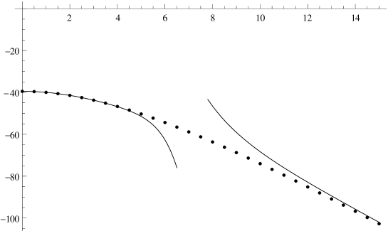
Figure 4: Spectral gap for ASEP with weak asymmetry $1-q=\mu/\sqrt{L}$ (WASEP) in the limit $L\to\infty$. The dots are the result of the extrapolation method applied on finite size Bethe ansatz numerics. The solid curve at small $\mu$ is $\sum_{j=0}^{5}d_{j}\,\mu^{2j}$ with the $d_{j}$’s given by (50). The solid curve at large $\mu$ is $e_{1}^{\mathrm{TASEP}}\mu+c_{1}\mu^{-2}+c_{2}\mu^{-4}$.

5 Conclusions

We have shown in this paper that ASEP and TASEP have exactly the same fluctuations on the relaxation scale, which confirms that KPZ universality extends to the whole crossover between short time transient fluctuations and stationary fluctuations. This result follows from high precision evaluations of asymptotics of eigenvalues and eigenvectors using extrapolation methods on finite size Bethe ansatz numerics. The eigenvalues and eigenvectors of ASEP and TASEP are conjectured to be essentially the same, which leads to several formulas (27), (29)-(35) for asymptotics of ASEP eigenstates.

We believe that proving these conjectured asymptotics would be a necessary first step in probing the crossover between equilibrium and KPZ fluctuations, which occurs in the weakly asymmetric regime $1-q\sim 1/\sqrt{L}$. Exact calculations for ASEP are however much more complicated than their counterparts for TASEP because of more complicated Bethe ansatz equations, and because of the presence of determinants that are not of Vandermonde type in the scalar products of Bethe vectors.

The extrapolation methods used in this paper to check the asymptotics should be useful for many other integrable models, at least in order to check asymptotic expressions, or even to guess new formulas as illustrated in the case of the spectral gap for ASEP with weak asymmetry.

Appendix A Algebraic Bethe ansatz for ASEP

In this appendix, we summarize briefly the algebraic Bethe ansatz construction of the eigenstates of the generator of ASEP as products of creation operators acting on a reference state. For more details, we refer to [2].

The creation operators, $B$ and $C$, are built from the monodromy matrix

$$\mathbb{T}_{a}(\mu)=\mathbb{L}_{aL}(\mu)\ldots\mathbb{L}_{a2}(\mu)\mathbb{L}_{a1}(\mu)=\left(\begin{array}[]{cc}A(\mu)&B(\mu)\\ C(\mu)&D(\mu)\end{array}\right)\;.$$ (52)

The monodromy matrix acts on the space $V_{a}\otimes V_{1}\otimes\ldots\otimes V_{L}$ with $V_{i}$, $i=1,\ldots,L$ the two-dimensional vector space corresponding to the site $i$ of an exclusion process, and $V_{a}$ an auxiliary space, also taken two-dimensional here. The space $V_{i}$ is generated by the vectors $|1\rangle_{i},|0\rangle_{i}$, corresponding respectively to an occupied site and to an empty site. The Lax operator $\mathbb{L}_{ai}(\mu)$ acts non-trivially only on the auxiliary site $a$ and on site $i$. Its local matrix in the basis $(|1\rangle_{a}\otimes|1\rangle_{i},|1\rangle_{a}\otimes|0\rangle_{i},|0\rangle_{a}\otimes|1\rangle_{i},|0\rangle_{a}\otimes|0\rangle_{i})$ is

$$\mathbb{L}_{ai}(\mu)=\left(\begin{array}[]{cccc}1&0&0&0\\ 0&\rme^{\gamma}\frac{1-\mu}{1-q\mu}&\frac{1-q}{1-q\mu}&0\\ 0&\frac{(1-q)\mu}{1-q\mu}&q\,\rme^{-\gamma}\frac{1-\mu}{1-q\mu}&0\\ 0&0&0&1\end{array}\right)\;.$$ (53)

It can be shown that

$$|\psi\rangle=C(y_{1})\ldots C(y_{N})|\emptyset\rangle\;$$ (54)

is an eigenvector of $M(\gamma)$ if the Bethe roots $y_{1}$, …, $y_{N}$ are solution of the Bethe equations (4). The reference state $|\emptyset\rangle$ corresponds to the configuration with no particles. The left eigenvectors are built similarly, using the creation operators $B(y)$ instead,

$$\langle\psi|=\langle\emptyset|B(y_{1})\ldots B(y_{N})\;.$$ (55)

A key point for the integrability of ASEP is that the Lax operators satisfy the Yang-Baxter equation

$$\mathbb{R}_{ab}(\mu/\nu)\mathbb{L}_{a}(\mu)\mathbb{L}_{b}(\nu)=\mathbb{L}_{a}(\nu)\mathbb{L}_{b}(\mu)\mathbb{R}_{ab}(\mu/\nu)\;,$$ (56)

with $\mathbb{R}_{ab}(\mu)=\mathbb{P}_{ab}\mathbb{L}_{ab}(\mu)$ and $\mathbb{P}_{ab}$ the operator permuting the two auxiliary sites $a$ and $b$. By construction, the Yang-Baxter equation also holds when replacing Lax operators $\mathbb{L}$ by monodromy matrices $\mathbb{T}$, which implies that the transfer matrix

$$T(\mu)=\tr_{a}\mathbb{T}_{a}(\mu)=A(\mu)+D(\mu)\;$$ (57)

verifies the commutation relation $T(\mu)T(\nu)=T(\nu)T(\mu)$ for all $\mu$, $\nu$. The existence of this commuting family of operators, to which belongs the deformed Markov matrix $M(\gamma)=T^{\prime}(0)T^{-1}(0)$, is at the heart of the integrability of ASEP. In particular, (54) and (55) are eigenvectors of $T(\mu)$ for all $\mu$, with eigenvalue $E(\mu)$ defined in (11).

The Yang-Baxter equation gives a quadratic algebra for the operators $A$, $B$, $C$, $D$ defined in (52), in particular $B(\mu)B(\nu)=B(\nu)B(\mu)$ and $C(\mu)C(\nu)=C(\nu)C(\mu)$, which means that the order of the operators in (54) and (55) does not matter: the eigenvectors are symmetric functions of the Bethe roots. Explicit expressions for the components of the eigenvectors for configurations with particles at positions $x_{j}$, $j=1,\ldots,N$, are given by the coordinate form of the Bethe ansatz (7), (8), see e.g. [38] for a derivation from (54), (55).

Appendix B Numerical solution of the Bethe equations

In this appendix, we explain the method used in this paper to solve numerically the Bethe equations (4). The method has two steps: we first solve the Bethe equations for TASEP using their simple structure when $q=0$. We then use the TASEP result as a starting point for solving the Bethe equations of ASEP for a small value of $q$, and then iterate up to a target value with $0<q<1$. Two iteration procedures are considered, either formulating the problem as a system of differential equations obtained by taking the derivative of the Bethe equations with respect to $q$, or using multidimensional Newton’s method for solving directly the Bethe equations.

B.1 First step: TASEP

At $q=0$, taking both sides of the Bethe equations (4) to the power $1/L$ gives

$$g(y_{j})=\rme^{\frac{2\rmi\pi k_{j}}{L}-b}\;,$$ (58)

where the $k_{j}$’s, distinct modulo $L$, characterize the eigenstates. The $k_{j}$’s are integers (half-integers) if $N$ is odd (even). The function $g$ is defined by

$$g(y)=\frac{1-y}{y^{\rho}}\;,$$ (59)

and $b$ is solution of

$$b-\gamma=\frac{1}{L}\sum_{j=1}^{N}\log y_{j}\;.$$ (60)

This last equation can be solved numerically for $b$ using Newton’s method, repeatedly replacing $b$ by

$$b_{\mathrm{new}}=b-\frac{b-\gamma-\frac{1}{L}\sum_{j=1}^{N}\log y_{j}(b)}{\frac{1}{N}\sum_{j=1}^{N}\frac{y_{j}(b)}{\rho+(1-\rho)y_{j}(b)}}\;$$ (61)

until the desired precision is reached. At each step, the $y_{j}(b)$, $j=1,\ldots,N$ are computed by inverting $g$ in (58) also using Newton’s method: $y=g^{-1}(z)$ is obtained by repeatedly replacing $y$ with

$$y_{\mathrm{new}}=\frac{1+\rho-\rho\,y-z\,y^{\rho}}{1-\rho+\rho/y}\;.$$ (62)

B.2 Second step: ASEP (from derivatives with respect to $q$)

In order to solve the Bethe equations for ASEP, one can consider the $y_{j}$’s as functions of $q$ and take the derivative of the logarithm of Bethe equations (4) with respect to $q$. We obtain the system of $N$ ordinary differential equations

$$\hskip 28.45274pt-\frac{y_{j}^{\prime}}{1-y_{j}}+\frac{1}{L}\sum_{k=1}^{N}\frac{y_{j}+qy_{j}^{\prime}-y_{k}^{\prime}}{qy_{j}-y_{k}}=-\frac{y_{j}+qy_{j}^{\prime}}{1-qy_{j}}+\frac{1}{L}\sum_{k=1}^{N}\frac{y_{j}^{\prime}-y_{k}-qy_{k}^{\prime}}{y_{j}-qy_{k}}\;,$$ (63)

where $y_{j}^{\prime}$ is the derivative of $y_{j}$ with respect to $q$. We write $\mathbf{y}\,^{\prime}(q)=f(q,\mathbf{y}(q))$ and evolve (63) from the TASEP solution $\mathbf{y}(0)$ to a target value $q$ in $M$ steps with increments $\delta q=q/M$ using the modified midpoint method. It consists in writing approximations $Y_{m}$ of $\mathbf{y}(m\delta q)$, $m=0,\ldots,M$ calculated iteratively by $Y_{0}=\mathbf{y}(0)$, $Y_{1}=Y_{0}+\delta qf(0,Y_{0})$ and $Y_{m+1}=Y_{m-1}+2\delta qf(m\delta q,Y_{m})$, $m=1,\ldots,M-1$. Then, one chooses as approximation for $\mathbf{y}(q)$ the quantity $\mathbf{y}^{M}(q)=\mbox{\small$\frac{1}{2}$}(Y_{M-1}+Y_{M}+\delta qf(q,Y_{M}))$. The crucial point is that the error from the modified midpoint method has a large $M$, fixed $q$ asymptotic expansion of the form $\mathbf{y}^{M}(q)-\mathbf{y}(q)\simeq\sum_{\ell=1}^{\infty}a_{\ell}M^{-2\ell}$ if the integer $M$ is even. Applying the modified midpoint method several times for $M=2,4,\ldots,2K$, it is then possible to use the extrapolation described in section 4 to estimate the value of $\mathbf{y}(q)$. The combination of the modified midpoint method and rational Richardson extrapolation, usually called the Bulirsch-Stoer method, is a classical method for solving ordinary differential equations with high precision, i.e. several hundreds or thousands of digits.

B.3 Second step: ASEP (from multidimensional Newton’s method)

An alternative method to solve the Bethe equations for ASEP is to use Newton’s method iteratively, and increase $q$ slowly enough so that one does not end up with another solution of the Bethe equations. Once one has reached the target value $q$, one can apply Newton’s method again with higher precision. Each step of the multidimensional Newton’s method used here consists in replacing the $y_{j}$’s with $y_{j}^{\mathrm{new}}$’s solution of the linear system

$$\hskip 14.22636pt\sum_{k=1}^{N}(y_{k}^{\mathrm{new}}-y_{k})\Bigg{[}\delta_{j,k}\Big{(}\frac{1}{1-y_{j}}-\frac{q}{1-qy_{j}}\Big{)}+\frac{\delta_{j,k}}{L}\sum_{\ell=1}^{N}\Big{(}\frac{1}{y_{j}-qy_{\ell}}-\frac{q}{qy_{j}-y_{\ell}}\Big{)}$$ (64)

$$\hskip 19.91692pt+\frac{1}{L}\Big{(}\frac{1}{qy_{j}-y_{k}}-\frac{q}{y_{j}-qy_{k}}\Big{)}\Bigg{]}=\frac{1}{L}\log\Bigg{[}-\rme^{L\gamma}\Big{(}\frac{1-y_{j}}{1-qy_{j}}\Big{)}^{L}\prod_{\ell=1}^{N}\frac{qy_{j}-y_{\ell}}{y_{j}-qy_{\ell}}\Bigg{]}\;.$$

This second method, although much cruder than the one of B.2, performs in practice very well.

References

- [1] B. Derrida. Non-equilibrium steady states: fluctuations and large deviations of the density and of the current. J. Stat. Mech., 2007:P07023, 2007.
- [2] O. Golinelli and K. Mallick. The asymmetric simple exclusion process: an integrable model for non-equilibrium statistical mechanics. J. Phys. A: Math. Gen., 39:12679–12705, 2006.
- [3] K. Johansson. Shape fluctuations and random matrices. Commun. Math. Phys., 209:437–476, 2000.
- [4] C.A. Tracy and H. Widom. Total current fluctuations in the asymmetric simple exclusion process. J. Math. Phys., 50:095204, 2009.
- [5] B. Derrida and J.L. Lebowitz. Exact large deviation function in the asymmetric exclusion process. Phys. Rev. Lett., 80:209–213, 1998.
- [6] D.S. Lee and D. Kim. Large deviation function of the partially asymmetric exclusion process. Phys. Rev. E, 59:6476–6482, 1999.
- [7] M. Kardar, G. Parisi, and Y.-C. Zhang. Dynamic scaling of growing interfaces. Phys. Rev. Lett., 56:889–892, 1986.
- [8] T. Kriecherbauer and J. Krug. A pedestrian’s view on interacting particle systems, KPZ universality and random matrices. J. Phys. A: Math. Theor., 43:403001, 2010.
- [9] T. Sasamoto and H. Spohn. The 1+1-dimensional Kardar-Parisi-Zhang equation and its universality class. J. Stat. Mech., 2010:P11013, 2010.
- [10] J. Quastel and H. Spohn. The one-dimensional KPZ equation and its universality class. J. Stat. Phys., 160:965–984, 2015.
- [11] T. Halpin-Healy and K.A. Takeuchi. A KPZ cocktail-shaken, not stirred… J. Stat. Phys., 160:794–814, 2015.
- [12] P.L. Ferrari. From interacting particle systems to random matrices. J. Stat. Mech., 2010:P10016, 2010.
- [13] I. Corwin. The Kardar-Parisi-Zhang equation and universality class. Random Matrices: Theory and Applications, 1:1130001, 2011.
- [14] B. Derrida and C. Appert. Universal large-deviation function of the Kardar-Parisi-Zhang equation in one dimension. J. Stat. Phys., 94:1–30, 1999.
- [15] E. Brunet and B. Derrida. Probability distribution of the free energy of a directed polymer in a random medium. Phys. Rev. E, 61:6789–6801, 2000.
- [16] A.M. Povolotsky, V.B. Priezzhev, and Chin-Kun Hu. The asymmetric avalanche process. J. Stat. Phys., 111:1149–1182, 2003.
- [17] M. Gorissen, A. Lazarescu, K. Mallick, and C. Vanderzande. Exact current statistics of the asymmetric simple exclusion process with open boundaries. Phys. Rev. Lett., 109:170601, 2012.
- [18] S. Prolhac. Finite-time fluctuations for the totally asymmetric exclusion process. Phys. Rev. Lett., 116:090601, 2016.
- [19] J. Baik and Z. Liu. arXiv 1605.07102, 2016.
- [20] R.P. Langlands and Y. Saint-Aubin. Algebro-geometric aspects of the Bethe equations. In Strings and Symmetries, volume 447 of Lecture Notes in Physics, pages 40–53. Berlin: Springer, 1995.
- [21] R.P. Langlands and Y. Saint-Aubin. Aspects combinatoires des équations de Bethe. In Advances in Mathematical Sciences: CRM’s 25 Years, volume 11 of CRM Proceedings and Lecture Notes, pages 231–302. Amer. Math. Soc., 1997.
- [22] E. Brattain, N. Do, and A. Saenz. The completeness of the Bethe ansatz for the periodic ASEP. arXiv:1511.03762, 2015.
- [23] M. Gaudin, B.M. McCoy, and T.T. Wu. Normalization sum for the Bethe’s hypothesis wave functions of the Heisenberg-Ising chain. Phys. Rev. D, 23:417–419, 1981.
- [24] V.E. Korepin. Calculation of norms of Bethe wave functions. Commun. Math. Phys., 86:391–418, 1982.
- [25] K. Motegi, K. Sakai, and J. Sato. Long time asymptotics of the totally asymmetric simple exclusion process. J. Phys. A: Math. Theor., 45:465004, 2012.
- [26] S. Prolhac. Asymptotics for the norm of Bethe eigenstates in the periodic totally asymmetric exclusion process. J. Stat. Phys., 160:926–964, 2015.
- [27] N.A. Slavnov. Calculation of scalar products of wave functions and form factors in the framework of the algebraic Bethe ansatz. Theor. Math. Phys., 79:502–508, 1989.
- [28] B. Pozsgay. Overlaps between eigenstates of the XXZ spin-1/2 chain and a class of simple product states. J. Stat. Mech., 2014:P06011, 2014.
- [29] J. Mossel and J.-S. Caux. Relaxation dynamics in the gapped XXZ spin-1/2 chain. New J. Phys., 12:055028, 2010.
- [30] N.M. Bogoliubov. Determinantal representation of the time-dependent stationary correlation function for the totally asymmetric simple exclusion model. SIGMA, 5:052, 2009.
- [31] L.-H. Gwa and H. Spohn. Six-vertex model, roughened surfaces, and an asymmetric spin Hamiltonian. Phys. Rev. Lett., 68:725–728, 1992.
- [32] S. Prolhac. Spectrum of the totally asymmetric simple exclusion process on a periodic lattice - first excited states. J. Phys. A: Math. Theor., 47:375001, 2014.
- [33] J. de Gier and F.H.L. Essler. Exact spectral gaps of the asymmetric exclusion process with open boundaries. J. Stat. Mech., 2006:P12011, 2006.
- [34] D. Kim. Bethe ansatz solution for crossover scaling functions of the asymmetric XXZ chain and the Kardar-Parisi-Zhang-type growth model. Phys. Rev. E, 52:3512–3524, 1995.
- [35] S. Prolhac. Current fluctuations and large deviations for periodic TASEP on the relaxation scale. J. Stat. Mech., 2015:P11028, 2015.
- [36] K.K. Kozlowski. On condensation properties of Bethe roots associated with the XXZ chain. arXiv:1508.05741, 2015.
- [37] M. Henkel and G.M. Schütz. Finite-lattice extrapolation algorithms. J. Phys. A: Math. Gen., 21:2617–2633, 1988.
- [38] O. Golinelli and K. Mallick. Derivation of a matrix product representation for the asymmetric exclusion process from the algebraic Bethe ansatz. J. Phys. A: Math. Gen., 39:10647–10658, 2006.