Opening the Frey/Osborne Black Box: Which Tasks of a Job are Susceptible to Computerization?

Abstract

In their seminal paper, Frey and Osborne quantified the automation of jobs, by assigning each job in the O*NET database a probability to be automated. In this paper, we refine their results in the following way: Every O*NET job consists of a set of tasks, and these tasks can be related. We use a linear program to assign probabilities to tasks, such that related tasks have a similar probability and the tasks can explain the computerization probability of a job. Analyzing jobs on the level of tasks helps comprehending the results, as experts as well as laymen can more easily criticize and refine what parts of a job are susceptible to computerization.

I Introduction

Computerization is considered to be one of the biggest socio-economic challenges. What is the foundation of the recent worries about many jobs being affected by automation [BM12, FO13, BM14, For15]?

Why did the last few years see dramatic technological progress regarding self-driving cars [Gui11], board games [SHM⁺16], automatic language translation [AGQZ13], or face recognition [Le13]? One reason is big data. While “intelligent algorithms” in the past were restricted to learning from data sets with a few thousand examples, we now have exabytes of data. Learning becomes even more powerful if you combine big data with a highly parallel hardware, stirred by the success of graphics processing units (GPUs). However, both of these technological advancements needed to be harvested, and they are with the advent of so-called deep learning algorithms, which have blown the competition away, starting with voice recognition [DYH09]. As a consumer, you can already witness some of these advancements on your smartphone, but a lot more is to come soon. We believe that these advancements will revolutionize white collar work and (with a little help from sensors and robotics) also blue collar work. In contrast to previous waves of innovation, this time new emerging jobs might not be able to compensate jobs endangered by the new technology.

In their seminal paper, Frey and Osborne [FO13] quantitatively study job automation, predicting that 47% of US employment is at risk of automation. In order to calculate this number, Frey and Osborne labeled 70 of the 702 jobs from the O*NET OnLine job database manually as either “automatable” or “not automatable”. Then, for the remainder of the jobs in the O*NET database, they computed the automation probability as a function of the distance to the labeled jobs.

But the results of Frey and Osborne are opaque, one either believes their “magic” computerization percentages, or one has doubts. We want anybody to be able to easily understand and argue about our results, by incorporating the unique tasks of each job. This additional depth will help laymen as well as job experts to argue about potential flaws in our methodology.

If we know that a job is 100% automatable, we also know that every task of that job must be completely automatable. But what if a job is 87% automatable? Is every task 87% automatable? Or are 87% of the tasks completely automatable, and 13% not at all? We want to forecast which tasks of a job are safe and which tasks are automatable.

In order to calculate the automation probability for a task, we first need to determine its share of a job (Section IV). Based on this, we are able to assign each task a probability to be automated such that the weighted average of the probabilities is equal to the probability of the corresponding job (Section VI-A). During our evaluation (Section VI-B), we discover a few suspicious results in the probabilities by Frey and Osborne, e.g., a surprisingly high automation probability of 96% for the job compensation and benefits managers. We conclude our paper by analyzing the correlation between various properties of a job and its probability to be automated (Section VII). E.g., we show that there is a strong negative correlation between the level of education required for a job and its probability to be automated.

Our complete results can be found at http://jobs-study.ethz.ch.

II Related Work

The current effects of automation have been studied intensively in economics. Most studies agree that some routine tasks have already fallen victim to automation [ALM01, GM07, AD09]. A task is routine if “it can be accomplished by machines following explicit programmed rules” [ALM01]. With computers being able to do routine tasks, the demand for human labor performing these tasks has decreased. But on the other hand, the demand for college educated labor has increased over the last decades [BJ89, Woo94, Woo98]. The effect is more pronounced in industries that are computer-intensive [AKK97]. As a consequence of this, the employment share of the highest skill quartile has increased. In addition to more people being employed in the highest skill quartile, the real wage for this quartile has increased faster than the average real wage. Service occupations, which are non-routine, but also not well paid, have also seen an increase in employment share and in real hourly wage. Thus, both, employment share and real wage, are U-shaped with respect to the skill level [AD09]. This employment pattern is a phenomenon that is called polarization. This is not unique to the US, but can also be observed, e.g., in the UK [GM07]. These papers make important observations about the effects that automation already has. Until now, routine tasks are the ones most affected, but more and more tasks can nowadays be performed by a computer. We focus on the future and try to predict which tasks will be automated next.

John Keynes predicted already in 1933 that there will be widespread technological unemployment “due to the means of economising the use of labour outrunning the pace at which we can find new uses for labour” [Key33]. Automation might be the technology, where this becomes true [BM12, FO13, BM14, For15]. “Automation of knowledge work”, “Advanced robotics”, and “Autonomous and near-autonomous vehicles” are considered to be 3 out of 12 potentially economically disruptive technologies [MCB⁺13]. Computer labor and human labor may no longer be complements, but competitors. Automation might be the cause for the current stagnation [BM12]. There might be too much technological progress, which causes high unemployment. A trend that could be going on for years, but was hidden by the housing boom [CHN13].

The seminal paper by Frey and Osborne is the first to make quantitative claims about the future of jobs [FO13]. Together with 70 machine learning experts, Frey and Osborne first manually labeled 70 out of 702 jobs from the O*NET database as either “automatable” or “non automatable”. This labeling was, as the authors admit, a subjective assignment based on “eye balling” the job descriptions from O*NET. Labels were only assigned to jobs where the whole job was considered to be (non) automatable, and to jobs where the participants of the workshop were most confident. To calculate the probability for non-labeled jobs, Frey and Osborne used a probabilistic classification algorithm. They chose 9 properties from O*NET as features for their classifier, namely “Finger Dexterity”, “Manual Dexterity”, “Cramped Work Space, Awkward Positions”, “Originality”, “Fine Arts”, “Social Perceptiveness”, “Negotiation”, “Persuasion”, and “Assisting and Caring for Others”.

The results from Frey and Osborne for the US job market were adopted to other countries, e.g., Finland, Norway, and Germany [PE15, BGZ15]. This was done by matching each job from O*NET to the locally used standardized name. Due to differences in the economies, a different percentage of people will be affected by this change, e.g., only one third in Finland and Norway are at risk compared to 47% in the US.

III Model

We are given a set of jobs $J=\{j_{1},\ldots,j_{n}\}$. Each job $j_{i}$ consists of a set of tasks $T_{i}=\{t_{i}^{1},\ldots,t_{i}^{m}\}$, where every task belongs to exactly one job. We call two tasks $t_{i}^{k}$ and $t_{i^{\prime}}^{k^{\prime}}$ related if and only if these tasks are similar according to O*NET. Two jobs with related tasks are also called related. An example with 3 jobs is depicted in Figure 1.

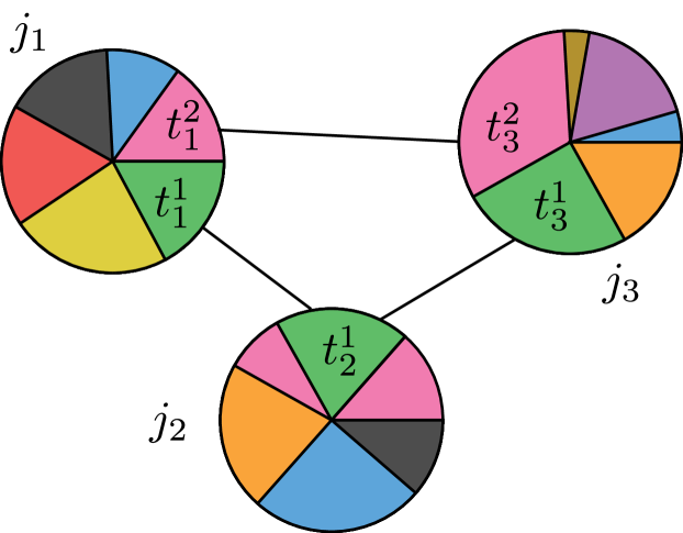
Figure 1: This figure shows a small example consisting of three jobs represented by circles. The share of each task of a job is shown by its sector. Two tasks are connected by a line if and only if they are related, i.e., similar according to O*NET. Task $t_{1}^{1}$ from job $j_{1}$ and task $t_{2}^{1}$ from job $j_{2}$ are related as indicated by the line connecting them. Note that this relationship is not transitive. Thus, tasks $t_{1}^{1}$ and $t_{3}^{1}$ do not need to be related.

O*NET provides us for each task $t_{i}^{k}$ with the information how often it is performed. This information was gathered by asking job incumbents and occupational experts. The options are “yearly or less”, “more than yearly”, “more than monthly”, “more than weekly”, “daily”, “several times daily”, and “hourly or more”. O*NET provides a percentage for each of the 7 options. We denote these frequencies of task $t_{i}^{k}$ with $f_{1}(t_{i}^{k}),\ldots,f_{7}(t_{i}^{k})$. Since these values are percentages, for every task $t_{i}^{k}$ they sum up to 100%, i.e., $\sum_{\ell=1}^{7}{f_{\ell}(t_{i}^{k})}=1$.

Each job $j_{i}$ has a given probability $p(j_{i})$ to be automated. We want to use $p(j_{i})$ to calculate a probability to be automated for each task of this job.

IV From Task Frequencies to Task Shares

We use the frequencies with which a task is performed to assign each task $t_{i}^{k}$ its share $s(t_{i}^{k})$. For every task $t_{i}^{k}$, the share denotes how much time is spent doing this task, such that $\sum_{t_{i}^{k}\in T_{i}}s(t_{i}^{k})=1$. The frequency values from O*NET do not fulfill this property; their values are very consistent for one job, but they can vary a lot between different jobs and might even seem to contradict each other. An extreme example can be seen in Figure 2. The seven frequency options provided by O*NET are on the $x$-axis and on the $y$-axis is the corresponding value of each option.

To make use of the high consistency within a job, we decided that the share of a task is a weighted average of its frequencies, i.e., $s(t_{i}^{k}):=\sum_{\ell=1}^{7}x_{i}^{\ell}f_{\ell}(t_{i}^{k})$. We want to calculate the job specific coefficients $x_{i}^{\ell}$. Let us illustrate these coefficients with a simple example. If $x_{i}^{7}=0.1$, then a task $t_{i}^{k}$ that is done exclusively “hourly or more” (i.e., $f_{7}(t_{i}^{k})=1$) makes up 10% of job $j_{i}$.

We want these coefficients to satisfy a few assumptions. If O*NET states that a task is done “hourly or more”, then the share of this task should be higher than the share of a task that is done “several times daily”. This translates to $x_{i}^{\ell}\leq x_{i}^{\ell+1}$ $\forall\ell\in\{1,\ldots,6\}$ and $0\leq x_{i}^{1}$.

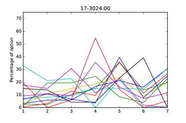
(a) Electro-Mechanical Technicians

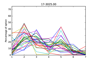
(b) Environmental Engineering Technicians

Figure 2: The number of tasks and the frequencies assigned to them can differ significantly even for related jobs.

These constraints neither use that jobs are related nor do they define the coefficients uniquely. Both issues are solved if we require the coefficients $x_{i}^{\ell}$ and $x_{i^{\prime}}^{\ell}$ for two related jobs $j_{i}$ and $j_{i^{\prime}}$ to be similar. The intuition behind this is that the frequencies of O*NET for related jobs are not independent of each other either, but rather should be similar as well. Occupational experts who have rated the frequency in which a task is done for one job, are likely to have rated the frequencies of related jobs.

The coefficients cannot be identical without violating the other constraints. Jobs have a different number of tasks and the frequencies are task specific. The example in Figure 2 highlights this. It is therefore easy to see that we cannot have the same coefficients for two related jobs and fulfill the equality $\sum_{t_{i}^{k}\in T_{i}}s(t_{i}^{k})=1$ for both jobs simply because the number of tasks can differ a lot.

Thus, we allow a bit of slack in the coefficients of related jobs. We use the variable $x_{i,i^{\prime}}^{\ell}$ to express the difference between the coefficients $x_{i}^{\ell}$ and $x_{i^{\prime}}^{\ell}$ for two related jobs $j_{i},j_{i^{\prime}}$. Formally, we define it as $x_{i,i^{\prime}}^{\ell}:=\max\{x_{i}^{\ell}-x_{i^{\prime}}^{\ell},x_{i^{\prime}}^{\ell}-x_{i}^{\ell}\}$. This yields the following linear program, which minimizes the overall slack:

minimize $$\sum x_{i,i^{\prime}}^{\ell}$$

s.t.

$$x_{i,i^{\prime}}^{\ell}\geq x_{i}^{\ell}-x_{i^{\prime}}^{\ell} \forall\ell$$

$$\forall j_{i},j_{i^{\prime}}\in J\mbox{ that are related{}}$$

$$x_{i,i^{\prime}}^{\ell}\geq x_{i^{\prime}}^{\ell}-x_{i}^{\ell} \forall\ell$$

$$\forall j_{i},j_{i^{\prime}}\in J\mbox{ that are related{}}$$

$$\sum_{t_{i}^{k}\in T_{i}}\sum_{\ell=1}^{7}x_{i}^{\ell}f_{\ell}(t_{i}^{k})\leq 1+\varepsilon \forall j_{i}\in J$$

$$\sum_{t_{i}^{k}\in T_{i}}\sum_{\ell=1}^{7}x_{i}^{\ell}f_{\ell}(t_{i}^{k})\geq 1-\varepsilon \forall j_{i}\in J$$

$$x_{i}^{1}\geq 0 \forall j_{i}\in J$$

$$x_{i}^{\ell}\geq x_{i}^{\ell-1} \forall j_{i}\in J\qquad\ell\in\{2,\ldots,7\}$$

We set $\varepsilon$ to 0.01. The resulting LP has 169,372 variables in its objective function. Since there are $735$ jobs, this means that a job is related to approximately $32.9$ other jobs on average. The value of the objective function is $24.6$, i.e., for two related jobs the coefficients differ only by $0.000145$ on average. For comparison, the average value of a coefficient is $0.060$. Our complete results can be found online at http://jobs-study.ethz.ch.

V From Jobs to Tasks

Knowing the shares of the tasks enables us to set up a linear program that calculates for each task the probability to be automated. We want that the weighted average of the automation probabilities $p(t_{i}^{k})$ of the tasks of a job $j_{i}$ can explain the automation probability $p(j_{i})$ of the job, i.e., $\sum_{t_{i}^{k}\in T_{i}}p\left(t_{i}^{k}\right)\cdot s\left(t_{i}^{k}\right)\approx p\left(j_{i}\right)$. Furthermore, we want to assign related tasks similar automation probabilities. To do this, we define a variable $t_{i,i^{\prime}}^{k,k^{\prime}}$ for each pair of related tasks $t_{i}^{k}$ and $t_{i^{\prime}}^{k^{\prime}}$. It denotes the probability difference that we assign to the two tasks. Formally, it is defined as $t_{i,i^{\prime}}^{k,k^{\prime}}:=\max\{p(t_{i}^{k})-p(t_{i^{\prime}}^{k^{\prime}}),p(t_{i}^{k})-p(t_{i^{\prime}}^{k^{\prime}})\}$. We want to minimize the sum of these variables, i.e., the sum of the probability difference of all related tasks.

Combining these requirements with necessary conditions to have meaningful probabilities, i.e., $0\leq p(t_{i}^{k})\leq 1$, yields the following linear program:

minimize $$\sum t_{i,i^{\prime}}^{k,k^{\prime}}$$

s.t.

$$p(t_{i}^{k})-p(t_{i^{\prime}}^{k^{\prime}})\leq t_{i,i^{\prime}}^{k,k^{\prime}} \forall t_{i}^{k},t_{i^{\prime}}^{k^{\prime}}\mbox{ that are related}$$

$$p(t_{i^{\prime}}^{k^{\prime}})-p(t_{i}^{k})\leq t_{i,i^{\prime}}^{k,k^{\prime}} \forall t_{i}^{k},t_{i^{\prime}}^{k^{\prime}}\mbox{ that are related}$$

$$\sum_{k}p(t_{i}^{k})\cdot s\left(t_{i}^{k}\right)\leq p(j_{i})\left(1+\varepsilon\right) \forall j_{i}\in J$$

$$\sum_{k}p(t_{i}^{k})\cdot s\left(t_{i}^{k}\right)\geq p(j_{i})\left(1-\varepsilon\right) \forall j_{i}\in J$$

$$p(t_{i}^{k})\geq 0 \forall j_{i}\in J,t_{i}^{k}\in T_{i}$$

$$p(t_{i}^{k})\leq 1 \forall j_{i}\in J,t_{i}^{k}\in T_{i}$$

$$t_{i,i^{\prime}}^{k,k^{\prime}}\geq 0 \forall t_{i,i^{\prime}}^{k,k^{\prime}}$$

$$t_{i,i^{\prime}}^{k,k^{\prime}}\leq 1 \forall t_{i,i^{\prime}}^{k,k^{\prime}}$$

We set $\varepsilon$ to $0.01$.

VI Linear Program Results

We now analyze the results of the linear program as described above. Later on, we will look at a small refinement to automatically detect outliers in our results.

VI-A Task Probabilities

The linear program as described in Section V has 105,748 variables in its objective function and it has a minimal value of 9,846. This means that two related tasks differ, on average, with regard to their probability by $9.3\%$. The complete results can be found online at http://jobs-study.ethz.ch. The histogram of the probability difference between two related tasks is shown in Figure 3. A majority of related tasks is assigned a similar probability. A small fraction of related tasks is assigned diametrically opposed probabilities, which seems startling. It can be reconciled by considering that neither the classification by Frey and Osborne nor the classification of tasks being related by O*NET are perfect.

Figure 3: A histogram of the probability with which two related tasks differ.

One example that highlights this are the two jobs computer programmer and software developers, applications. These two jobs have many related tasks, but the probabilities of these jobs differ a lot (4% for software developers, applications, 48% for computer programmers). Hence, the diametrically opposed probabilities are necessary to meet the constraints of the linear program.

In the following, we present a few selected jobs to illustrate our results. The first example is chemists. This job has an automation probability of 10% according to Frey and Osborne. Only one task has, according to our linear program, a high probability of being automated: “Induce changes in composition of substances by introducing heat, light, energy, or chemical catalysts for quantitative or qualitative analysis.” Other simple mechanical tasks have been assigned low automation probabilities. We will revisit this job in Section VI-B.

Next up: judges. Their automation probability is 40%. The tasks, their probabilities, and their shares are shown in Table 4. The tasks that can be automated can be grouped in two sets: preliminary hearings which includes making first assessments, and ensuring that the procedures in court are followed. The tasks that involve sentencing (or the preparation thereof) have been assigned low automation probabilities.

Task Description	$p$	Share
Write decisions on cases.	1	5.1
Instruct juries on applicable laws, direct juries to deduce the facts from the evidence presented, and hear their verdicts.	1	3.4
Monitor proceedings to ensure that all applicable rules and procedures are followed.	1	8.0
Advise attorneys, juries, litigants, and court personnel regarding conduct, issues, and proceedings.	1	6.2
Interpret and enforce rules of procedure or establish new rules in situations where there are no procedures already established by law.	1	5.4
Conduct preliminary hearings to decide issues such as whether there is reasonable and probable cause to hold defendants in felony cases.	1	3.9
Rule on admissibility of evidence and methods of conducting testimony.	0.94	5.3
Preside over hearings and listen to allegations made by plaintiffs to determine whether the evidence supports the charges.	0.46	5.9
Perform wedding ceremonies.	0.39	2.7
Read documents on pleadings and motions to ascertain facts and issues.	0	10.1
Research legal issues and write opinions on the issues.	0	6.5
Settle disputes between opposing attorneys.	0	4.6
Participate in judicial tribunals to help resolve disputes.	0	6.6
Rule on custody and access disputes, and enforce court orders regarding custody and support of children.	0	6.3
Sentence defendants in criminal cases, on conviction by jury, according to applicable government statutes.	0	4.0
Grant divorces and divide assets between spouses.	0	4.7
Award compensation for damages to litigants in civil cases in relation to findings by juries or by the court.	0	3.8
Supervise other judges, court officers, and the court’s administrative staff.	0	8.5

Table 4: The automation probability and the share of each task of Judges, Magistrate Judges, and Magistrates”. The automation probability of this job is 40%.

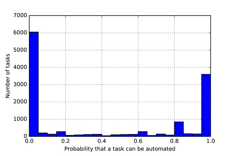
Figure 5: A histogram of the probabilities that tasks can be automated. Nearly all tasks are assigned either 0 or 1. This simplifies arguing whether our classification is correct.

Figure 5 shows the histogram of the probabilities from our linear program. The probabilities for most tasks are either very high or very low and only a few tasks have a probability in-between. This desired side effect of our linear program helps us to achieve our goal of allowing job experts (and laymen) to argue about the validity of our results. We invite the reader to have a look at other jobs at http://jobs-study.ethz.ch.

VI-B Outlier Detection

To evaluate our approach and check for outliers, we use a variant of cross-validation. For every job $j_{i}$, we create a linear program without job $j_{i}$. This yields a probability $p_{i}(\cdot)$ for every task but the tasks from $j_{i}$. Afterward, we calculate the new probability $p^{\prime}(j_{i})$ that job $j_{i}$ can be automated. We do this by setting the probability $p^{\prime}(t_{i}^{k})$ of each task $t_{i}^{k}$ to the average of all tasks that are related to it. We denote the set of related tasks by $N(t_{i}^{k})$. Formally, we set $p^{\prime}(t_{i}^{k}):=\frac{1}{|N(t_{i}^{k})|}\sum_{t_{i^{\prime}}^{k^{\prime}}\in N(t_{i}^{k})}p_{i}(t_{i^{\prime}}^{k^{\prime}})$.

We first compare $p^{\prime}(t_{i}^{k})$ with $p(t_{i}^{k})$. The difference between these two probabilities should be small for the majority of the tasks. This is indeed what can be seen in Figure 6. The histogram of $p^{\prime}(t_{i}^{k})-p(t_{i}^{k})$ shows that nearly all tasks have similar probabilities in both approaches. The average absolute difference is less than $20\%$. The distribution is centered around 0. Its mean is less than $0.05\%$.

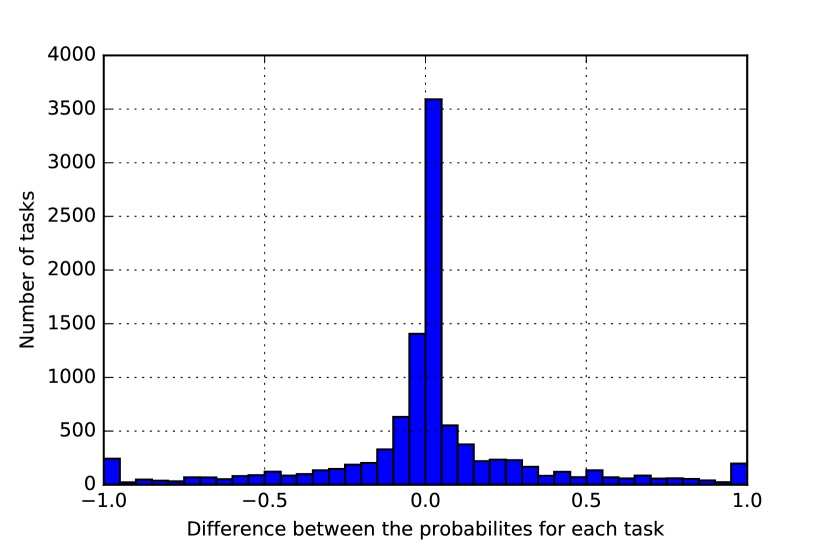
Figure 6: A histogram of $p(t_{i}^{k})-p^{\prime}(t_{i}^{k})$ for all tasks. This plot shows that most tasks have a similar probability in both approaches. The values are sharply distributed around 0.

By combining the new probability of each task with its share, we can calculate the new probability of job $j_{i}$ by using a weighted average. This allows us to compare $p^{\prime}(j_{i})$ with $p(j_{i})$.

We have plotted this difference, i.e., $p(j_{i})-p^{\prime}(j_{i})$, in Figure 7. We can see that the difference is centered around 0%; with the average absolute difference being less than $20\%$. For more than half of the jobs our probability differs by less than 20% from Frey and Osborne [FO13]. Most interesting are the jobs whose probability differs significantly. We now have a look at a few of them.

There are jobs where our probability is more than 80% smaller than the one by Frey and Osborne. One job is compensation and benefits managers. We assigned it a probability $p^{\prime}(j)$ to be automated of $9.1\%$; compared to $p(j)=96\%$ by Frey and Osborne. We do not claim to know the true value, but we can look at the job and compare it to the probabilities of jobs we consider similar. Notice that this is conceptually similar to what our linear program does and thus might be biased. The tasks of this job are shown in Table 8. If we manually compare them to related tasks, we conclude that they do not seem to be automatable in the next few decades. We do favor our result over the result of Frey and Osborne.

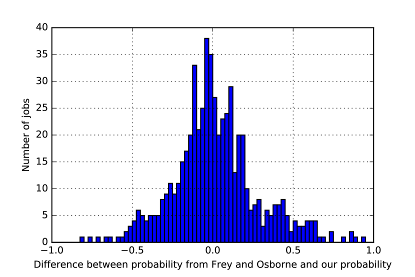
Figure 7: A histogram of the difference between the probability by Frey and Osborne with our probability. The distribution is centered around 0 and a majority of the jobs differs by less than 20%.

Task Description	$p$	$p^{\prime}$
Advise management on such matters as equal employment opportunity, sexual harassment and discrimination.	1	0.15
Study legislation, arbitration decisions, and collective bargaining contracts to assess industry trends.	1	0
Fulfill all reporting requirements of all relevant government rules and regulations, including the Employee Retirement Income Security Act (ERISA).	1	0.20
Investigate and report on industrial accidents for insurance carriers.	1	0.12
Represent organization at personnel-related hearings and investigations.	1	0
Analyze compensation policies, government regulations, and prevailing wage rates to develop competitive compensation plan.	1	0.5
Mediate between benefits providers and employees, such as by assisting in handling employees’ benefits-related questions or taking suggestions.	1	0.42
Prepare detailed job descriptions and classification systems and define job levels and families, in partnership with other managers.	1	0
Prepare personnel forecasts to project employment needs.	1	0
Direct preparation and distribution of written and verbal information to inform employees of benefits, compensation, and personnel policies.	1	0
Manage the design and development of tools to assist employees in benefits selection, and to guide managers through compensation decisions.	1	0
Design, evaluate and modify benefits policies to ensure that programs are current, competitive and in compliance with legal requirements.	1	0
Administer, direct, and review employee benefit programs, including the integration of benefit programs following mergers and acquisitions.	1	0
Prepare budgets for personnel operations.	1	0.03
Maintain records and compile statistical reports concerning personnel-related data such as hires, transfers, performance appraisals, and absenteeism rates.	1	0
Contract with vendors to provide employee services, such as food services, transportation, or relocation service.	1	0.38
Identify and implement benefits to increase the quality of life for employees, by working with brokers and researching benefits issues.	1	0
Plan, direct, supervise, and coordinate work activities of subordinates and staff relating to employment, compensation, labor relations, and employee relations.	1	0
Negotiate bargaining agreements.	1	0.67
Plan and conduct new employee orientations to foster positive attitude toward organizational objectives.	1	0
Conduct exit interviews to identify reasons for employee termination.	1	0
Develop methods to improve employment policies, processes, and practices, and recommend changes to management.	0.51	0
Formulate policies, procedures and programs for recruitment, testing, placement, classification, orientation, benefits and compensation, and labor and industrial relations.	0.23	0.01

Table 8: The tasks and their corresponding probability that they will be automated for Compensation and Benefits Managers according to our original linear program and the cross-validation.

There is only one job that we assign a much higher probability than Frey and Osborne. The job First-Line supervisors of production and operating workers has been assigned a 83% automation probability by us and only 1.6% by Frey and Osborne. A close inspection of the tasks makes us believe that the true value is between these extremes. Quite a few of the tasks are clearly automatable, e.g., “Keep records of employees’ attendance and hours worked.” and “Observe work and monitor gauges, dials, and other indicators to ensure that operators conform to production or processing standards.” Others, e.g., “Read and analyze charts, work orders, production schedules, and other records and reports to determine production requirements and to evaluate current production estimates and outputs.” seem difficult to automate. The complete results for this can job be found at http://jobs-study.ethz.ch.

We continue by comparing the previous results with the approach described in this section. To do this, we return to the jobs that we have looked at previously. First off is the job chemists. As shown in Table 9, the automation probability of most tasks has increased. Consequently, the automation probability of this job has increased from 10% to 42%. Due to the large difference, this job should be analyzed in-depth by job experts.

Task Description	$p$	$p^{\prime}$
Induce changes in composition of substances by introducing heat, light, energy, or chemical catalysts for quantitative or qualitative analysis.	0.68	0.82
Analyze organic or inorganic compounds to determine chemical or physical properties, composition, structure, relationships, or reactions, using chromatography, spectroscopy, or spectrophotometry techniques.	0.18	0.82
Maintain laboratory instruments to ensure proper working order and troubleshoot malfunctions when needed.	0.16	0.78
Conduct quality control tests.	0.07	0.54
Write technical papers or reports or prepare standards and specifications for processes, facilities, products, or tests.	0.03	0.03
Study effects of various methods of processing, preserving, or packaging on composition or properties of foods.	0	0.20
Prepare test solutions, compounds, or reagents for laboratory personnel to conduct tests.	0	0.63
Purchase laboratory supplies, such as chemicals, when supplies are low or near their expiration date.	0	1
Evaluate laboratory safety procedures to ensure compliance with standards or to make improvements as needed.	0	0
Direct, coordinate, or advise personnel in test procedures for analyzing components or physical properties of materials.	0	0.01
Develop, improve, or customize products, equipment, formulas, processes, or analytical methods.	0	0
Confer with scientists or engineers to conduct analyses of research projects, interpret test results, or develop nonstandard tests.	0	0.02

Table 9: The automation probability and the share of each task of a chemist.

The changes in the automation probability of the tasks of judges are much smaller. Most tasks have a similar automation probability as before and the overall probability of this job has changed marginally, i.e., increased only from 40% to 50%. Therefore, we are confident that the classification by Frey and Osborne is correct.

We conclude that our approach can also be used to detect outliers in the results of Frey and Osborne. We can then manually inspect the automation probabilities of the tasks of such an outlier to determine the truth. We think our results allow us to fine tune the results from Frey and Osborne, but not replace it, as we need their results to bootstrap our linear program.

VII Further Analysis

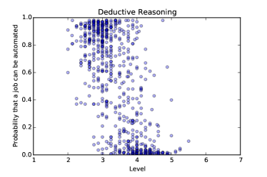
(a) Deductive Reasoning

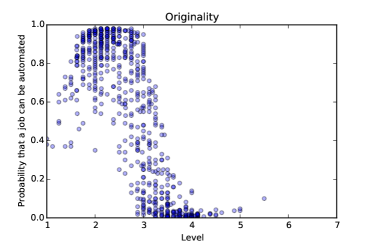
(b) Originality

Figure 10: The probability that a job can be automated over the level of the abilities “deductive reasoning” and “originality” used in this job. These levels are defined by O*NET and for each they provide an anchor point. Level 2 of “deductive reasoning” means “knowing that a stalled car can coast downhill” and level 5 “deciding what factors to consider in selecting stocks”. Level 2 of “originality” means “using a credit card to open a locked door” and level 6 “inventing a new type of man-made fiber”. Every point represents one job. A higher level of either of these two abilities correlates, as expected, with a lower probability to be automated.

In addition to inspecting every task of every job, we consider a broader picture. We do this by looking at general properties of a job that correlate with the probability that it can be automated.

VII-A Tasks

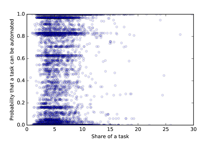
Figure 11: Our results show almost no correlation between the share of a task and its probability that it will be automated.

We first analyze the share of a task. The higher the share, the more often a task is performed. Hence, from a machine learning perspective this means that much more training data is available. This might lead to the conclusion that such a task is easier to automate. To disprove this claim, we plotted the share of a task over the probability that a task can be automated according to our linear program. The resulting graph is shown in Figure 11. Every dot represents one task, with its share on the $x$-axis and its probability on the $y$-axis. We see that there is barely any correlation between these two. We conclude that tasks that are done more frequently are not more likely to be automated.

VII-B Jobs

We continue our analysis by looking at the correlation between the properties that a job has, e.g., what kind of degree is necessary to do a job, and the probability that this job can be automated. Correlation does not imply causation, but nevertheless, these results reveal some interesting nuggets.

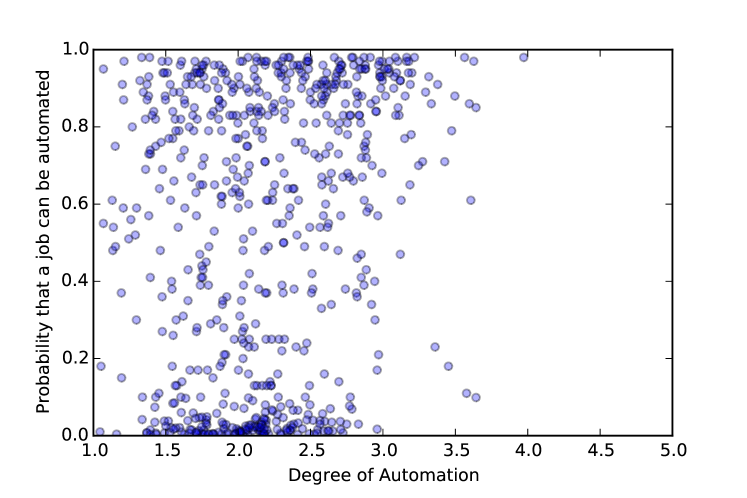
Figure 12: The probability that a job can be automated over the level of the current “Degree of Automation”. This level ranges from $1$ (Not at all automated) to $5$ (Completely automated). The rather small correlation of $0.23$ implies that different jobs will soon be affected.

O*NET provides the level that the ability “deductive reasoning” is used in a job. The level ranges from $1$ to $7$, where for example level 2 means “knowing that a stalled car can coast downhill” and level 5 “deciding what factors to consider in selecting stocks”. For every job, we have one value between $1$ and $7$. The resulting graph can be seen in Figure 10. Every job is represented by one dot; its $x$-coordinate being its level and the $y$-coordinate its probability. We can see that jobs that require a high level of deductive reasoning tend to have a lower probability of being automated.

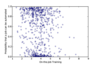
(a) On the Job Training

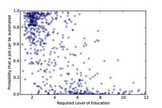
(b) Required Level of Education

Figure 13: The probability that a job can be automated over the amount of “On the Job Training” (ranging from 1 (none or short demonstration) to 9 (over 10 years) and the “Required of Level of Education” (ranging from 1 (less than a high school diploma) to 12 (post-doctoral training)).

A similar result can be seen for “originality” (see Figure 10). Level 2 of “originality” means “using a credit card to open a locked door” and level 6 means “inventing a new type of man-made fiber”. This confirms our expectation that these abilities will remain difficult for a computer.

O*NET even has an explicit value for the current level of the “degree of automation” for each job. This level ranges from $1$ (not at all automated) to $5$ (completely automated). As depicted in Figure 12, the already existing level of automation barely correlates with the probability that this job will be automated. This indicates that not only jobs that are already affected by automation are in danger, but also a whole new set of jobs. This is aligned with the recent worries about many new jobs soon being affected by computerization.

We conclude this section by looking at the effect that the level of required education for a job has on the probability to be automated. Jobs that require only very little education (level 1, i.e., less than a high school diploma) tend to have a higher probability than jobs that require an associate degree (level 5) which in turn have a higher probability than jobs that require post-doctoral training (level 12). Most jobs that require little education are in danger. It is noteworthy that the effect of training before the job is much stronger than the effect of on the job training. Jobs that require more on the job training only have a marginally smaller probability to be automated. Both plots are shown in Figure 13.

VIII Conclusion

We believe that automation is one of the main challenges for society. In our opinion, the seminal work of Frey and Osborne did an excellent job of getting the discussion going. In this paper we dug a bit deeper, by looking not only at jobs – but at the tasks that make up a job. We hope that opening the Frey/Osborne black box will help the discussion. The professionals that are actually doing a job are the main experts to decide what parts of their job can or cannot be computerized. The Frey/Osborne work only tells these experts that their job is 87% automatable, but what does it actually mean? With our work, job experts can look inside the box, and understand which tasks of their job are at risk. Our hope is that the job experts have a discussion which results are believable and which are not, and why. To facilitate this discussion, we have created a web page (http://jobs-study.ethz.ch) that allows users to comment upon our results.

References

- [AD09] David H. Autor and David Dorn. The growth of low skill service jobs and the polarization of the us labor market. Technical report, National Bureau of Economic Research, 2009.
- [AGQZ13] Michael Auli, Michel Galley, Chris Quirk, and Geoffrey Zweig. Joint language and translation modeling with recurrent neural networks. In EMNLP, volume 3, page 0, 2013.
- [AKK97] David H. Autor, Lawrence F Katz, and Alan B Krueger. Computing inequality: have computers changed the labor market? Technical report, National Bureau of Economic Research, 1997.
- [ALM01] David H Autor, Frank Levy, and Richard J Murnane. The skill content of recent technological change: An empirical exploration. Technical report, National Bureau of Economic Research, 2001.
- [BGZ15] Holger Bonin, Terry Gregory, and Ulrich Zierahn. Übertragung der Studie von Frey/Osborne (2013) auf Deutschland. Technical report, ZEW Kurzexpertise, 2015.
- [BJ89] John Bound and George E Johnson. Changes in the structure of wages during the 1980’s: An evaluation of alternative explanations. Technical report, National Bureau of Economic Research, 1989.
- [BM12] Erik Brynjolfsson and Andrew McAfee. Race against the machine: How the digital revolution is accelerating innovation, driving productivity, and irreversibly transforming employment and the economy. Brynjolfsson and McAfee, 2012.
- [BM14] Erik Brynjolfsson and Andrew McAfee. The second machine age: work, progress, and prosperity in a time of brilliant technologies. WW Norton & Company, 2014.
- [CHN13] Kerwin Kofi Charles, Erik Hurst, and Matthew J Notowidigdo. Manufacturing decline, housing booms, and non-employment. Technical report, National Bureau of Economic Research, 2013.
- [DYH09] L Deng, D Yu, and G Hinton. Deep learning for speech recognition and related applications. In NIPS Workshop, 2009.
- [FO13] Carl Benedikt Frey and Michael A. Osborne. The future of employment: How susceptible are jobs to computerisation?, 2013.
- [For15] Martin Ford. Rise of the Robots: Technology and the Threat of a Jobless Future. Basic Books, 2015.
- [GM07] Maarten Goos and Alan Manning. Lousy and lovely jobs: The rising polarization of work in britain. The review of economics and statistics, 89(1):118–133, 2007.
- [Gui11] Erico Guizzo. How google’s self-driving car works. IEEE Spectrum Online, October, 18, 2011.
- [Key33] John Maynard Keynes. Economic possibilities for our grandchildren (1930). Essays in persuasion, pages 358–73, 1933.
- [Le13] Quoc V Le. Building high-level features using large scale unsupervised learning. In ICASSP, pages 8595–8598. IEEE, 2013.
- [MCB+13] James Manyika, Michael Chui, Jacques Bughin, Richard Dobbs, Peter Bisson, and Alex Marrs. Disruptive technologies: Advances that will transform life, business, and the global economy, volume 12. McKinsey Global Institute New York, 2013.
- [PE15] Mika Pajarinen and Anders Ekeland. Computerization and the future of jobs in norway. 2015.
- [SHM+16] David Silver, Aja Huang, Christopher J. Maddison, Arthur Guez, Laurent Sifre, George van den Driessche, Julian Schrittwieser, Ioannis Antonoglou, Veda Panneershelvam, Marc Lanctot, Sander Dieleman, Dominik Grewe, John Nham, Nal Kalchbrenner, Ilya Sutskever, Timothy Lillicrap, Madeleine Leach, Koray Kavukcuoglu, Thore Graepel, and Demis Hassabis. Mastering the game of go with deep neural networks and tree search. Nature, 529:484–503, 2016.
- [Woo94] Adrian Wood. North-south trade, employment and inequality. New York, 1994.
- [Woo98] Adrian Wood. Globalisation and the rise in labour market inequalities. The economic journal, 108(450):1463–1482, 1998.