Dynamics of Hubbard Hamiltonians with the multiconfigurational time-dependent Hartree method for indistinguishable particles

Abstract

We apply the multiconfigurational time-dependent Hartree method for indistinguishable particles (MCTDH-X) to systems of bosons or fermions in lattices described by Hubbard type Hamiltonians with long-range or short-range interparticle interactions. The wavefunction is expanded in a variationally optimized time-dependent many-body basis generated by a set of effective creation operators that are related to the original particle creation operators by a time-dependent unitary transform. We use the time-dependent variational principle for the coefficients of this transform as well as the expansion coefficients of the wavefunction in the time-dependent many-body basis as variational parameters to derive equations of motion. The convergence of MCTDH-X is shown by comparing its results to the exact diagonalization of one-, two-, and three-dimensional lattices filled with bosons with contact interactions. We use MCTDH-X to study the buildup of correlations in the long-time splitting dynamics of a Bose-Einstein condensate loaded into a large two-dimensional lattice subject to a barrier that is ramped up in the center. We find that the system is split into two parts with emergent time-dependent correlations that depend on the ramping time – for most barrier-raising-times the system becomes two-fold fragmented, but for some of the very fast ramps, the system shows revivals of coherence.

I Introduction

Ultracold atoms in optical lattices are a very active and wide field of research that bridges the gap between atom-, molecular, and optical physics and condensed matter systems. They have been employed as quantum simulators for condensed matter systems that cannot be experimentally controlled to the same extent as ultracold atoms in optical lattices CB98 ; BH ; fer2 . Recent progress in this direction includes for instance the realization of artificial gauge fields gauge-exp and topological states of matter top-exp with cold atom systems.

To describe the dynamics of ultracold atoms in optical lattices theoretically requires solving the equation governing these systems, i.e., the time-dependent many-body Schrödinger equation (TDSE). However, the dimensionality of the many-body Hilbert space that hosts the solution grows exponentially with the number of particles and with the number of sites in the considered optical lattice. Since no general analytical solution is known to date, many approximate numerical methods have been devised. Popular approaches include the time-dependent density matrix renormalization group TDMRG , matrix product states MPS1 ; MPS2 ; MPS3 , time-evolved block decimation TEBD1 ; TEBD2 , dynamical mean-field theory FDMFT ; BDMFT ; DMFT-1st ; DMFT-MCTDH , mean-field lattice methods, the discrete nonlinear Schrödinger equation DNLS , and the Hartree-Fock theory for Hubbard Hamiltonians HubbardHF . These methods have problems when dealing with optical lattices of spatial dimension larger than one (time-dependent density matrix renormalization group, matrix product states, time-evolved block dimension), when the considered lattice is not spatially homogeneous (dynamical mean-field theory), or they oversimplify the emergent many-body correlations (discrete nonlinear Schrödinger equation and Hartree-Fock for Hubbard Hamiltonians).

For continuous systems of ultracold atoms, i.e., atoms that do not reside in an optical lattice, a theory which does not suffer from the aforementioned problems has been formulated alon ; MCTDHX and implemented exact_F ; MCTDH-X ; S-MCTDHB : the multiconfigurational time-dependent Hartree for indistinguishable particles. In this work, we apply the same philosophy to describe ultracold atoms in optical lattices.

We adopt the strategy of Refs. alon ; MCTDHX and apply the time-dependent variational principle DFVP ; TDVP to the time-dependent many-body Schrödinger equation using a formally complete, time-dependent, and variationally optimized orthonormal many-body basis set and demonstrate the exactness of the obtained theory, the multiconfigurational time-dependent Hartree method for indistinguishable particles in lattices (MCTDH-X). In the static case, i.e., the solution of the time-independent Schrödinger equation, we compare MCTDH-X for a bosonic Hamiltonian with exact diagonalization and find that the error in the obtained method goes to zero roughly exponentially with the number of effective time-dependent one-particle basis functions employed. In the dynamical case, i.e., the solution of the time-dependent Schrödinger equation, we apply MCTDH-X to the long-time splitting dynamics of bosons in a two-dimensional lattice. We show that correlations in the split system are built up almost independently of the splitting times: the reduced one-body density matrix acquires two eigenvalues on the order of the particle number throughout the splitting process, i.e., fragmentation emerges. Fragmentation emerges with a delay for short splitting times which becomes proportional to the splitting time for longer splitting times. Interestingly, revivals of the uncorrelated (coherent) initial state are seen for very short splitting times. By quantifying the coherence of the system with the first-order correlation function, we show that the mechanism behind the fragmentation is the loss of coherence between the left and right fractions of the bosons as the barrier is ramped up.

II Theory

II.1 Schrödinger equation and Hubbard Hamiltonians

The aim is to solve the time-dependent many-body Schrödinger equation,

$$i\partial_{t}|\Psi\rangle=\hat{H}|\Psi\rangle,$$ (1)

for the Hubbard Hamiltonian including a general long-ranged interaction,

$$\hat{H}_{\text{Hub}}=\sum_{j}\epsilon_{j}\hat{b}^{\dagger}_{j}\hat{b}_{j}-J\sum_{<j,k>}\left[\hat{b}^{\dagger}_{j}\hat{b}_{k}+\hat{b}^{\dagger}_{k}\hat{b}_{j}\right]+\frac{U}{2}\sum_{i\leq j}W(i,j)\left(\hat{b}^{\dagger}_{i}\right)^{2}\left(\hat{b}_{j}\right)^{2}.$$ (2)

Here and in the following, $<\cdot,\cdot>$ denotes neighboring sites. The full many-body state reads

$$|\Psi\rangle=\sum_{\{\vec{n}\}}C_{\vec{n}}(t)|\vec{n}\rangle;\qquad|\vec{n}\rangle=\sqrt{\frac{1}{n_{1}!\cdots n_{M_{s}}!}}\left(\hat{b}^{\dagger}_{1}\right)^{n_{1}}\cdots\left(\hat{b}^{\dagger}_{M_{s}}\right)^{n_{M_{s}}}|vac\rangle.$$ (3)

The sum in this ansatz runs over all possible configurations of $N$ indistinguishable particles in the $M_{s}$ lattice sites. In the exact diagonalization approach, one takes Eq. (3) as the ansatz and determines the coefficients $C_{\vec{n}}(t)$. However, the number of the coefficients $C_{\vec{n}}(t)$ in the many-body ansatz Eq. (3) grows as a factorial [$\binom{N+M_{s}-1}{N}$ for bosons and $\binom{M_{s}}{N}$ for fermions], i.e. exponentially, with the number of lattice sites.

To make large lattices tractable, approximations have to be introduced to reduce the number of coefficients. In what follows, we use a variational approach to obtain such an approximation: the general “MCTDH ansatz” is used to derive equations of motion.

II.2 MCTDH-X for Hubbard Hamiltonians

The MCTDH-X equations of motion are derived with a time-dependent variational principle of the Schrödinger equation TDVP for Hubbard Hamiltonians by taking into account multiple “effective” time-dependent creation operators that act on all $M_{s}$ lattice sites.

To start, we note that one can transform the time-independent operators $\hat{b}^{\dagger}_{j}$ in the Hubbard Hamiltonian in Eq. (2) using a time-dependent unitary matrix $u_{kj}(t)$ to a set of $M$ operators $\{a^{\dagger}_{k}(t)\}$,

$$\hat{a}^{\dagger}_{k}\equiv\sum_{j=1}^{M_{s}}u_{kj}(t)\hat{b}^{\dagger}_{j},$$ (4)

with the inverse transformation

$$\hat{b}^{\dagger}_{j}=\sum_{k=1}^{M}u^{*}_{kj}\hat{a}^{\dagger}_{k}(t).$$ (5)

It is important to note that in the above equation $M$ is the number of effective creation operators $\hat{a}_{k}(t)$ considered and is not the number of sites $M_{s}$ in the system. To proceed, one forms all possible configurations $\vec{m}$ of $N$ particles in $M$ of the above effective time-dependent operators $\hat{a}^{\dagger}_{k}(t)$. The resulting ansatz for the many-body state then reads

$$|\Psi\rangle = \sum_{\vec{n}}C_{\vec{n}}(t)|\vec{n}\rangle\equiv\sum_{\vec{m}}C_{\vec{m}}(t)|\vec{m};t\rangle$$ (6)

$$|\vec{m};t\rangle = \sqrt{\frac{1}{m_{1}!\cdots m_{M}!}}\left(\hat{a}^{\dagger}_{1}(t)\right)^{m_{1}}\cdots\left(\hat{a}^{\dagger}_{M}(t)\right)^{m_{M}}|vac\rangle.$$ (7)

The number of coefficients $C_{\vec{m}}(t)$ that has to be accounted for is $\binom{N+M-1}{N}$ for bosons and $\binom{M}{N}$ for fermions. The number of coefficients is no longer directly dependent on the number of sites $M_{s}$ in the treated system. Note that the multiconfigurational ansatz in Eq. (6) contains the mean-field type wavefunctions of the time-dependent Hartree-Fock for fermions and the so called discrete non-linear Schrödinger equation for bosons as special cases, for $M=N$ and $M=1$, respectively. The action functional TDVP ; DFVP for the time-dependent many-body Schrödinger equation (1) can now be (re-)formulated using the operator relation in Eq. (5) and reads

$$S[\{u_{kj}\},\{u^{*}_{kj}\}]=\int dt\left(\langle\Psi(t)|\hat{H}_{\text{Hub}}-i\partial_{t}|\Psi(t)\rangle-\sum_{pq}\mu_{pq}(t)\left[\sum_{j}u^{*}_{pj}(t)u_{qj}(t)-\delta_{pq}\right]\right).$$ (8)

Here, the time-dependent Lagrange multipliers $\mu_{pq}(t)$ have been introduced to enforce the orthonormality of the column vectors of the transform $u_{pk}(t)$. This ensures that $u_{pk}(t)$ is indeed unitary for all times $t$. To derive the equations of motion for $u_{pk}(t)$, we proceed by inserting the transformed operators given in Eq. (5) in the above action, Eq. (8):

$$\langle\Psi(t)|\hat{H}_{\text{Hub}}-i\partial_{t}|\Psi(t)\rangle=$$

$$\langle\Psi(t)|\bigg{[}\sum_{j}\epsilon_{j}\sum_{pq}u^{*}_{pj}(t)u_{qj}(t)\hat{a}^{\dagger}_{p}(t)\hat{a}_{q}(t)-J\sum_{<j,k>}\sum_{pq}u^{*}_{pj}(t)u_{qk}(t)\hat{a}^{\dagger}_{p}(t)\hat{a}_{q}(t)$$

$$+ \frac{U}{2}\sum_{i\leq j}\sum_{prqs}W(i,j)u^{*}_{pj}(t)u^{*}_{rj}(t)u_{qj}(t)u_{sj}(t)\hat{a}^{\dagger}_{p}(t)\hat{a}^{\dagger}_{r}(t)\hat{a}_{q}(t)\hat{a}_{s}(t)$$

$$- i\sum_{j}\sum_{pq}u^{*}_{pj}(t)\partial_{t}u_{qj}(t)\hat{a}^{\dagger}_{p}(t)\hat{a}_{q}(t)|\Psi(t)\rangle-i\sum_{\vec{m}}C_{\vec{m}}^{*}\partial_{t}C_{\vec{m}}\bigg{]}|\Psi(t)\rangle.$$ (10)

With the abbreviations,

$$T_{pq} = -J\sum_{<k,s>}u^{*}_{pk}(t)u_{qs}(t)$$ (11)

$$V_{pq} = \sum_{j}\epsilon_{j}u^{*}_{pj}(t)u_{qj}(t)$$ (12)

$$\vec{W}_{rs} = U\sum_{j}u^{*}_{rj}(t)W(i,j)u_{sj}(t)$$ (13)

$$W_{rs_{pq}} = U\sum_{k,j}u^{*}_{pk}(t)u^{*}_{rj}(t)W(j,k)u_{qk}(t)u_{sj}(t)$$ (14)

$$\rho_{kq} = \langle\Psi(t)|\hat{a}^{\dagger}_{p}(t)\hat{a}_{q}(t)|\Psi(t)\rangle\>,$$ (15)

Eq. (10) reads

$$\langle\Psi(t)|\hat{H}_{\text{Hub}}-i\partial_{t}|\Psi(t)\rangle = \sum_{pq}\rho_{pq}\left(T_{pq}+V_{pq}-i\partial_{t_{pq}}\right)$$

$$+ \frac{1}{2}\sum_{pqrs}\rho_{prqs}W_{rs_{pq}}-i\sum_{\vec{m}}C^{*}_{\vec{m}}(t)\partial_{t}C_{\vec{m}}(t).$$

In the following, we use the vector notation $\vec{u}_{p}(t)$ for the column vectors of $u_{kj}(t)$ and refer to these vectors as orbitals. Furthermore, we use bold math symbols to denote matrices of the quantities defined in Eqs. (11) and (12). The variation of the action functional with respect to the orbitals $\{\vec{u}^{*}_{p}(t)\}$ can now be performed. Since the action takes on the same functional form as in the case of MCTDH-X, compare Eq. (II.2) to Eq. (10) in Ref. MCTDHX , the variation with respect to the orbitals $\{\vec{u}^{*}_{p}(t)\}$ also must have the same functional form as the equations of motion of MCTDH-X. They take on the form

$$i\partial_{t}\vec{u}_{j}(t) = \mathbf{\hat{P}}\left.\Bigg{(}\left[\mathbf{T}+\mathbf{V}\right]\vec{u}_{j}(t)\right.$$

$$+ \left.\sum_{k,s,q,l=1}^{M}\{\rho(t)\}^{-1}_{jk}\cdot\rho_{ksql}(t)\vec{W}_{sl}\vec{u}_{q}(t)\right.\Bigg{)};$$

$$\mathbf{\hat{P}} = \mathbf{1}-\sum_{j^{\prime}=1}^{M}\vec{u}_{j^{\prime}}(t)\left(\vec{u}^{*}_{j^{\prime}}(t)\right)^{T}.$$

for the orbitals and

$$\mathcal{H}(t)\mathcal{C}(t)=i\partial_{t}\mathcal{C}(t);\qquad\mathcal{H}_{\vec{m}\vec{m}^{\prime}}(t)=\langle\vec{m};t|\hat{H}-i\partial_{t}|\vec{m}^{\prime};t\rangle$$ (18)

for the coefficients, where a vector notation $\mathcal{C}(t)=\{C_{\vec{m}}(t)\}$ was introduced. The equations for the orbitals, Eq. (II.2), are presented here using the invariance property $\sum_{j}u_{qj}^{*}\partial_{t}u_{kj}=0$ that follows from the unitarity of $u_{kj}$.

The usage of the variational principle to derive equations of motion for multiconfigurational wavefunctions in lattices yields the same result as in the continuum case, but the equations contain a different and particular spatial representation of the potential and kinetic energy, namely the matrices $\mathbf{T}$ and $\mathbf{V}$ which encode that the considered many-body state lives in a lattice. The existing implementation of MCTDH-X exact_F ; MCTDH-X ; S-MCTDHB is straightforwardly adapted to the numerical solution of the equations of motion, Eqs. (18) and (II.2), the modifications concern $\mathbf{T}$ and $\mathbf{V}$ only.

Note that the projector $\mathbf{\hat{P}}$ above will vanish as soon as the basis $\{\vec{u}_{j};j=1,M\}$ is complete. This is exactly the case only, if the number of effective operators in the multiconfigurational ansatz is taken to be the number of sites in the lattice $M=M_{s}$. Then, the time derivative in the orbitals’ equations of motion (II.2) is zero and the case of exact diagonalization is recovered; Eq. (18) becomes equivalent to solving the TDSE with the full many-body state (3) and the Hubbard Hamiltonian (2). Furthermore, the equations of motion of MCTDH-X for Hubbard Hamiltonians, (II.2) and (18), boil down to the standard mean-field methods, i.e. the discrete non-linear Schrödinger equation in the case of $M=1$ and bosons and the time-dependent Hartree-Fock equations of motion in the case of $M=N$ and fermions. MCTDH-X for Hubbard Hamiltonians can hence be seen as a systematic generalization of mean-field methods: if the number of effective operators $M$ approaches the number of sites $M_{s}$ in the system the Hilbert space spanned by them is the full possible Hilbert space of the lattice. The variational principle used in the derivation of the approximation guarantees that the error in the description is minimal at any given point in time and, furthermore, once convergence is achieved even for a number of orbitals $M<M_{s}$, the dynamics of the full many-body wavefunction is captured Axel_exact ; Axel_book ; exact_F .

II.3 Quantities of interest

We introduce the quantities that will be used in the remainder of our work to analyze the obtained results. For notational convenience, we will write vectors as functions of position, for instance $\vec{u}_{k}\equiv u_{k}(\vec{r})$. The reduced one-body density matrix reads

$$\rho^{(1)}(\vec{r},\vec{r}^{\prime};t)=\sum_{kq}\rho_{kq}u_{k}^{*}(\vec{r}^{\prime};t)u_{q}(\vec{r};t).$$ (19)

The diagonal of the reduced one-body density matrix is the one-body density,

$$\rho(\vec{r})=\rho^{(1)}(\vec{r},\vec{r};t)=\sum_{kq}\rho_{kq}u_{k}^{*}(\vec{r};t)u_{q}(\vec{r};t).$$ (20)

To investigate correlations between the atoms, we use the fragmentation and the normalized first-order Glauber correlation functions $g^{(1)}$ Glauber .

Fragmentation is computed from the eigenvalues of the reduced one-body density matrix $\rho_{k}^{(NO)}$. These eigenvalues $\rho_{k}^{(NO)}$ are termed natural occupations and are obtained by diagonaling the reduced one-body density matrix, see Eq. (15). In a system with multiple natural occupations on the order of the number of particles, fragmentation can by quantified by

$$F(t)=\sum_{k=2}^{M}\rho_{k}^{(NO)}(t)=1-\rho_{1}^{(NO)}(t).$$ (21)

The quantity $F(t)$ defines what fraction of the atoms is outside the single particle state that corresponds to the largest eigenvalue $\rho_{1}^{(NO)}$ of the reduced one-body density matrix. The first-order Glauber correlation function,

$$g^{(1)}(\vec{r},\vec{r}^{\prime};t)=\frac{\rho^{(1)}(\vec{r},\vec{r}^{\prime};t)}{\sqrt{\rho(\vec{r};t)\rho(\vec{r}^{\prime};t)}},$$ (22)

is a measure for the spatial coherence and shows how well a product state can describe the reduced one-body density matrix $\rho^{(1)}(\vec{r},\vec{r}^{\prime};t)$ at $\vec{r},\vec{r}^{\prime}$: if a product state or mean-field description is applicable to the system, then $|g^{(1)}|^{2}=1$ holds, and if a product state of mean-field description is not applicable then $|g^{(1)}|^{2}<1$ is true. Note that the reduced one-body density matrix [Eq. (19)] can be transformed to momentum space by applying a Fourier transform to the orbitals $u_{k}(\vec{r};t)$. From the reduced density matrix in momentum space, the momentum density $\rho(\vec{k};t)$ and momentum correlations $g^{(1)}(\vec{k},\vec{k}^{\prime};t)$ can be computed in analogy to Eqs. (22) and (20), respectively.

III Results

We study the eigenstates and dynamics of bosons with contact interactions, i.e., $W(i,j)=\delta_{ij}$ in Eq. (2), in the following two Subsections.

III.1 Comparison with exact diagonalization

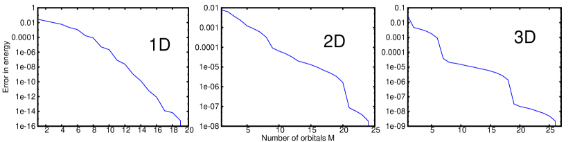
Figure 1: Comparison of MCTDH-X with exact diagonalization results. The relative error in the energies of $N=4,U=J=1$, harmonically trapped one-, two-, and three-dimensional bosons plotted in the left, middle, and right panel, respectively. In all cases the results converge roughly exponentially (note the logarithmic scale of the plots). All quantities shown are dimensionless.

To demonstrate the correctness of our implementation of the MCTDH-X method, we compare with exact diagonalization results for a bosonic system in one-, two-, and three-dimensional lattices of $20$, $5$ by $5$, and $3$ by $3$ by $3$ sites, respectively. For the parameters in the Hamiltonian, Eq. (2), we choose a harmonic on-site energy $\epsilon_{j}=\frac{1}{2}\omega^{2}\vec{r}_{j}^{2}$ and an interparticle interaction of $U=J=1$. We set the frequency $\omega$ of the external harmonic confinement to $0.1$, $1$, and $3$ for the one-, two-, and three-dimensional comparison with exact diagonalization, respectively. Figure 1 shows a plot of the error in the energies as a function of the number of orbitals $M$ in the computation. From the roughly exponential convergence of the error in energy to zero, we infer that the derived method indeed recovers the full complexity of the many-body state $|\Psi\rangle$ as the number of variational parameters in the description is increased. This means that the description of the Hubbard system with the introduced effective creation operators $\{\hat{a}^{\dagger}_{k}\}_{k=1}^{M}$ becomes complete and hence the solution of the MCTDH-X equations of motion, Eqs. (II.2) (18), is equivalent to the solution of the Schrödinger equation, Eq. (1). The time-dependent variational principle DFVP ; TDVP and the MCTDH-X method exact_F ; Axel_exact ; Axel_book ; S-MCTDHB imply the formal exactness of the approach.

III.2 Dynamical splitting of a two-dimensional superfluid

To assess that MCTDH-X can yield highly accurate predictions also for dynamics in large lattices, we study the splitting dynamics of a two-dimensional, initially parabolically trapped system of $N=100$ atoms in a $50$ by $50$ lattice with on-site repulsion $U=0.01J$. The size of the configuration space of this system, $N_{c}=\binom{N+M_{s}-1}{N}=\binom{100+2500-1}{100}\approx 4.7\cdot 10^{182}$ is far out of reach of exact diagonalization. In our simulations with MCTDH-X, we use $M=4$ effective operators and hence $\binom{N+M-1}{N}=\binom{100+4-1}{100}=176851$ configurations to describe the system. Since our results are converged with respect to the number of variational parameters, i.e., for the results for $M=3$ and $M=4$ all plots shown below are indistinguishable, our results can be considered as a numerically exact description of the on-going dynamics. The split is done by a Gaussian barrier in the center of the external harmonic confinement. The on-site energy offset is given by

$$\epsilon_{j}=\frac{1}{2}\omega_{\text{ext}}^{2}\vec{r}^{2}_{j}+V(t)\exp{\left(-\frac{x_{j}^{2}}{2\sigma^{2}}\right)}.$$ (23)

Here $\omega_{\text{ext}}$ is the frequency of the external harmonic trapping potential, $V(t)$ is the time-dependent height of the barrier and $\sigma$ its width. For our simulations we choose the value $\omega_{\text{ext}}=0.3$, $\sigma=1$, and a linear ramp for the barrier $V(t)$,

$$V(t)=\left\{\begin{array}[]{ll}\frac{t}{t_{\text{ramp}}}V_{\text{max}},&t\leq t_{\text{ramp}}\\ V_{\text{max}},&t>t_{\text{ramp}}\end{array}\right..$$ (24)

As a first step in our investigation, we choose an intermediate ramping time $t_{\text{ramp}}=50$, and analyze the time-evolution of the density. Fig. 2 shows a plot of the spatial and momentum densities at representative times. The spatial density $\rho(\vec{r};t)$ of the system is divided equally between the two wells by the split. Furthermore, the splitting is a non-adiabatic process, as there are remaining dynamics for $t>t_{\text{ramp}}$ after the split is complete: the maxima of the density in the left and the right minimum of the potential oscillate. The (Gaussian) momentum density $\rho(\vec{k};t)$ is spread out in the $x$-direction. During the splitting process for $t\in[0,t_{\text{ramp}}]$, the momentum density $\rho(\vec{k};t)$ shows multiple peaks, similar to the peaks that are observed in the ground states of bosons in a double-well in continuous space at intermediate barrier heights (cf. Fig. 3 in Ref. RDMs ). We move on and monitor the emergence of fragmentation, i.e., the macroscopic occupation of more than one natural orbital in the splitting process as a function of the time within which the barrier is ramped up to its maximal value $V_{\text{max}}$ to split the Bose-Einstein condensate. To quantify fragmentation, we plot the fraction $F(t)$ of particles outside of the lowest natural orbital of the system for barrier-raising-times $t_{\text{ramp}}\in\left[2,200\right]$ in Fig. 3. Fragmentation emerges for all the investigated ramp times $t_{\text{ramp}}$. The delay of the emerging fragmentation for longer ramp times is proportional to $t_{\text{ramp}}$, but constant at about $50$ time units in the case of short ramps $t_{\text{ramp}}\lesssim 40$. For very short ramps with $t_{\text{ramp}}\approx 5$, revivals of the initial fragmentation $F\approx 0$ are seen in the dynamics. This bears some resemblance of the inverse regime discussed in Ref. Split for the splitting of a one-dimensional Bose-Einstein condensate that does not reside in an optical lattice potential, where it was found that the system stays coherent counter-intuitively for larger interparticle repulsion at a fixed $t_{\text{ramp}}$. In the present case of the splitting of a Bose-Einstein condensate with an optical lattice potential, we find that the system retains its coherence for very fast ramps at fixed and small interparticle interactions. This behavior is counterintuitive as one would naively expect that a process that is further from being adiabatic and closer to a quench ($t_{\text{ramp}}\longrightarrow 0$) is more likely to break the coherence and drive the system to fragmentation. To get a space- and momentum-resolved picture of the emergence of fragmentation and the entailed loss of coherence, we pick a ramping time of $t_{\text{ramp}}=50$ and analyze the Glauber correlation function $g^{(1)}$ in the course of the splitting process in Fig. 4. Initially, at $t=0$ the atoms form a single connected superfluid: all atoms are coherent and $|g^{(1)}|^{2}=1$ in both real and momentum space. During the splitting process, spatial coherence is preserved only within the left and within the right well, respectively. The spatial coherence between the atoms in the left and right well is lost as fragmentation emerges with time (see $|g^{(1)}|\approx 0$ regions in the top row of Fig. 4). Fragmentation shows also in the momentum correlation functions: throughout the splitting process, a periodic diagonal line pattern of alternating coherent and incoherent momenta emerges (bottom row of Fig. 4).

IV Conclusions and outlook

In this work, we formulated a general many-body theory to describe dynamics and correlations of indistinguishable interacting many-body systems in lattices. The software implementation of our theory is openly available as part of the MCTDH-X software package MCTDH-X . We demonstrate that the method converges exponentially towards the exact result by comparing it to exact diagonalization.

We obtain numerically exact results for the long-time splitting dynamics of initially condensed bosonic atoms in a large two-dimensional optical lattice: correlations that manifest as the macroscopic dynamical occupation of two natural orbitals are built up on a time-scale that is proportional to the barrier-raising-time $t_{\text{ramp}}$ – the system becomes two-fold fragmented. Revivals of the initial coherence and absence of fragmentation is seen for very short ramping times.

As an outlook, we mention a detailed investigation of the observed counter-intuitive revivals as well as the application of MCTDH-X to many-body systems of atoms with internal degrees of freedom S-MCTDHB and/or systems subject to artificial gauge fields gauge-exp ; top-exp and spin-orbit interactions spielmanSOC ; song:SOCfrag .

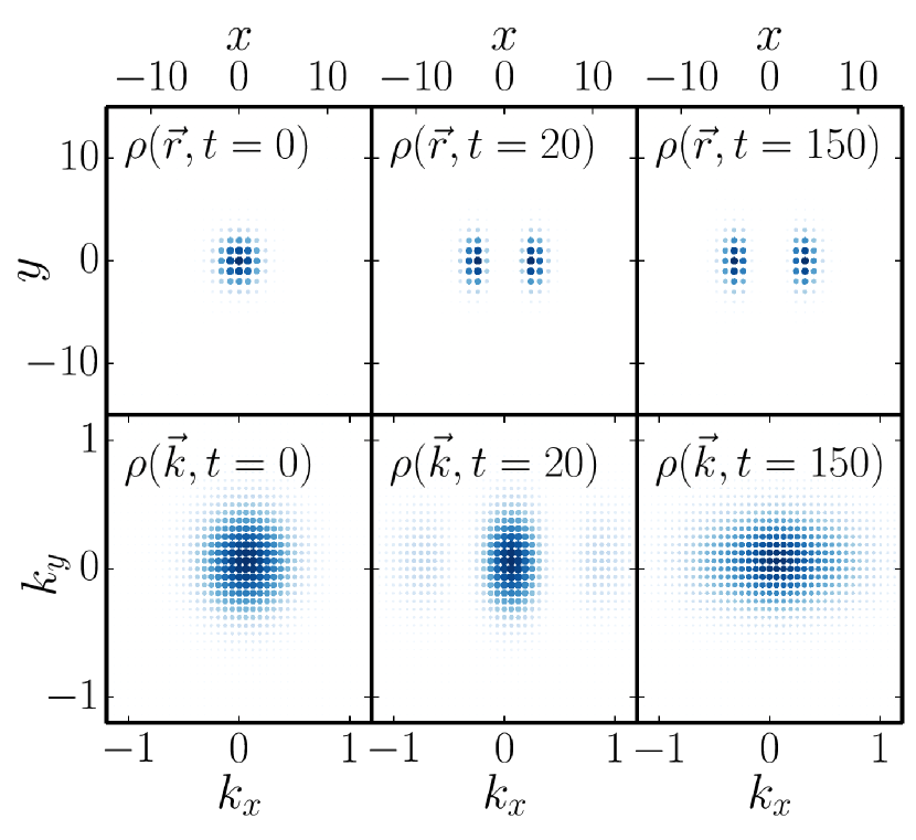
Figure 2: Spatial and momentum densities in the splitting process with $t_{\text{ramp}}=50$. The top row depicts the spatial density $\rho(\vec{r};t)$ and the bottom row depicts the momentum density $\rho(\vec{k};t)$ for times $t=0,20$, and $150$, respectively. Darker color and larger points stand for larger on-site density. The plot of $\rho(\vec{r};t)$ shows that the initially Gaussian density distribution is split in two equal parts by the barrier. The left and right maxima of the density oscillate even for $t>t_{\text{ramp}}$ when the barrier has fully been ramped up: the process is non-adiabatic. The momentum density $\rho(\vec{k};t)$ exhibits an initially Gaussian distribution. During the splitting process, around $t=20$, $\rho(\vec{k};t)$ has three maxima which recombine to a broadened Gaussian distribution, once the splitting is complete and fragmentation has emerged [see $\rho(\vec{k};t=150)$ in the lower row and Fig. 3]. All quantities shown are dimensionless.

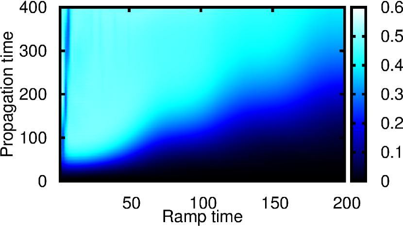
Figure 3: Emergence of fragmentation in the splitting of a two-dimensional Bose-Einstein condensate in a lattice. The fragmentation of the system is shown as a function of the propagation time and the barrier-raising time $t_{\text{ramp}}$. Generally, fragmentation takes longer to set in for larger values of $t_{\text{ramp}}$, but there is a threshold for very fast ramps; for short barrier-raising-times $t_{\text{ramp}}\lesssim 40$, the system needs about $50$ time units to become fragmented. For very short ramps $t_{\text{ramp}}\in\left[4,10\right]$, revivals of coherence are seen where the fragmentation returns back close to zero ($F=0$) after some propagation time. All quantities shown are dimensionless, see text for discussion.

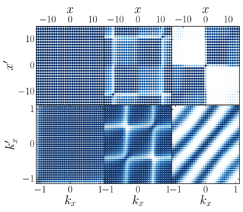
Figure 4: Loss of spatial and momentum coherence in the splitting process with $t_{\text{ramp}}=50$. The top row shows the real-space correlation function $|g^{(1)}(\vec{r}=(x,0),\vec{r}^{\prime}=(x^{\prime},0);t)|^{2}$ and the bottom row depicts the momentum space correlation function $|g^{(1)}(\vec{k}=(k_{x},0),\vec{k}^{\prime}=(k_{x}^{\prime},0);t)|^{2}$ for times $t=0,20$, and $150$, in the left, middle, and right columns, respectively. The darkest colors and biggest points correspond to $|g^{(1)}|=1$ (coherence) and white means $|g^{(1)}|=0$ (incoherence). Initially, at $t=0$, the bosons form a fully spatially- and momentum-coherent ensemble (see left column). In the course of the splitting process, spatial coherence is maintained only within the formed minima of the double-well potential, while the coherence between the atoms in the left and right minima of the potential is lost and $|g^{(1)}|^{2}$ vanishes on the off-diagonal blocks (see emerging “white squares” in top middle and top right panels). In momentum space, the loss of coherence between the atoms in the left and right well shows by the emergence of a periodic diagonal stripe pattern (see lower row). All quantities shown are dimensionless.

References

- (1) D. Jaksch, C. Bruder, J. I. Cirac, C. W. Gardiner, and P. Zoller, Cold Bosonic Atoms in Optical Lattices, Phys. Rev. Lett. 81, 3108 (1998).
- (2) M. Greiner, O. Mandel, T. Esslinger, T. W. Hänsch, and Immanuel Bloch, Quantum phase transition from a superfluid to a Mott insulator in a gas of ultracold atoms, A Mott insulator of fermionic atoms in an optical lattice, Nature 415, 39 (2002).
- (3) R. Jördens, N. Strohmaier, K. Günter, H. Moritz, and T. Esslinger, A Mott insulator of fermionic atoms in an optical lattice, Nature 455, 204 (2008).
- (4) J. Struck, M. Weinberg, C. Ölschläger, P. Windpassinger, J. Simonet, K. Sengstock, R. Höppner, P. Hauke, A. Eckardt, M. Lewenstein, and L. Mathey, Engineering Ising-XY spin-models in a triangular lattice using tunable artificial gauge fields, Nature Phys. 9, 738 (2013).
- (5) P. Hauke, O. Tielemann, A. Celi, C. Ölschläger, J. Simonet, J. Struck, M. Weinberg, P. Windpassinger, K. Sengstock, M. Lewenstein, and A. Eckardt, Non-Abelian Gauge Fields and Topological Insulators in Shaken Optical Lattices, Phys. Rev. Lett. 109, 145301 (2012).
- (6) U. Schollwöck, The density-matrix renormalization group, Rev. Mod. Phys. 77, 259 (2005).
- (7) G. Evenbly and G. Vidal, Entanglement Renormalization in Two Spatial Dimensions, Phys. Rev. Lett. 102, 180406 (2009).
- (8) F. Verstraete and J. I. Cirac, Matrix product states represent ground states faithfully, Phys. Rev. B 73, 094423 (2006).
- (9) F. Verstraete, M. M. Wolf, D. Perez-Garcia, and J. I. Cirac, Criticality, the Area Law, and the Computational Power of Projected Entangled Pair States, Phys. Rev. Lett. 96, 220601 (2006).
- (10) M. Zwolak and G. Vidal, Mixed-State Dynamics in One-Dimensional Quantum Lattice Systems: A Time-Dependent Superoperator Renormalization Algorithm, Phys. Rev. Lett. 93, 207205 (2004).
- (11) J. Kajala, F. Massel, and P. Törmä, Expansion Dynamics in the One-Dimensional Fermi-Hubbard Model, Phys. Rev. Lett. 106, 206401 (2011).
- (12) A. Geißler, I. Vasić, and W. Hofstetter, Condensation versus Long-range Interaction: Competing Quantum Phases in Bosonic Optical Lattice Systems at Near-resonant Rydberg Dressing, arxiv:1509.06292 (2015); K. M. Stadler, Z. P. Yin, J. von Delft, G. Kotliar, and A. Weichselbaum, Dynamical Mean-Field Theory Plus Numerical Renormalization-Group Study of Spin-Orbital Separation in a Three-Band Hund Metal, Phys. Rev. Lett. 115, 136401 (2015).
- (13) M. Eckstein, M. Kollar, and P. Werner, Thermalization after an Interaction Quench in the Hubbard Model, Phys. Rev. Lett. 103, 056403 (2009).
- (14) A. Georges, G. Kotliar, W. Krauth, and M. J. Rozenberg, Dynamical mean-field theory of strongly correlated fermion systems and the limit of infinite dimensions, Rev. Mod. Phys. 68, 13 (1996).
- (15) K. Balzer, Z. Li, O. Vendrell, and M. Eckstein, Multiconfiguration time-dependent Hartree impurity solver for nonequilibrium dynamical mean-field theory, Phys. Rev. B 91, 045136 (2015).
- (16) L. Pitaevskii and S. Stringari, Bose-Einstein Condensation (Clarendon University Press, Oxford (2003)).
- (17) V. Bach, E. H. Lieb, and J. P. Solovej, Generalized Hartree-Fock theory and the Hubbard model, J. Stat. Phys. 76, 3 (1994).
- (18) O. E. Alon, A. I. Streltsov, and L. S. Cederbaum, Multiconfigurational time-dependent Hartree method for bosons: Many-body dynamics of bosonic systems, Phys. Rev. A 77, 033613 (2008).
- (19) O. E. Alon, A. I. Streltsov, and L. S. Cederbaum, Unified view on multiconfigurational time propagation for systems consisting of identical particles, J. Chem. Phys. 127, 154103 (2007).
- (20) A. U. J. Lode, M. C. Tsatsos, and E. Fasshauer, MCTDH-X package: The time-dependent multiconfigurational Hartree for indistinguishable particles, http://ultracold.org (2016).
- (21) E. Fasshauer and A. U. J. Lode, The multiconfigurational time-dependent Hartree for fermions: Implementation, exactness, and few-fermion tunneling to open space, Phys. Rev. A 93, 033635 (2016).
- (22) A. U. J. Lode, The multiconfigurational time-dependent Hartree method for bosons with internal degrees of freedom, arXiv:1602.05791 (2016).
- (23) J. Frenkel, P. A. M. Dirac, Wave mechanics, Oxford Univ. Press, Oxford 435 (1934); ibid. Proc. Cambridge Phil. Soc., 26, 376 (1930).
- (24) P. Kramer and M. Saraceno, Geometry of the Time-Dependent Variational Principle in Quantum Mechanics, Lecture Notes in Physics 140, (Springer, Heidelberg, 1981).
- (25) A. U. J. Lode, K. Sakmann, O. E. Alon, L. S. Cederbaum, and A. I. Streltsov, Numerically exact quantum dynamics of bosons with time-dependent interactions of harmonic type, Phys. Rev. A 86, 063606 (2012).
- (26) A. U. J. Lode, Tunneling Dynamics in Open Ultracold Bosonic Systems, Springer Theses, Springer, Heidelberg (2014).
- (27) R. J. Glauber, The Quantum Theory of Optical Coherence, Phys. Rev. 130, 2529 (1963).
- (28) O. Penrose and L. Onsager, Bose-Einstein Condensation and Liquid Helium, Phys. Rev. 104, 576 (1956).
- (29) K. Sakmann, A. I. Streltsov, O. E. Alon, and L. S. Cederbaum, Reduced density matrices and coherence of trapped interacting bosons, Phys. Rev. A 78, 023615 (2008).
- (30) A. I. Streltsov, O. E. Alon, and L. S. Cederbaum, Role of Excited States in the Splitting of a Trapped Interacting Bose-Einstein Condensate by a Time-Dependent Barrier, Phys. Rev. Lett. 99, 030402 (2007).
- (31) Y.-J. Lin, K. Jiménez-García, I. B. Spielman, Spin-orbit-coupled Bose-Einstein condensates, Nature 471, 83–86 (2011).
- (32) S.-W. Song, Y.-C. Zhang, H. Zhao, X. Wang, and W.-M. Liu, Fragmentation of spin-orbit-coupled spinor Bose-Einstein condensates, Phys. Rev. A 89, 063613 (2014).