Neutrinos and $\gamma$-rays from the Galactic Center Region After H.E.S.S. Multi-TeV Measurements

Abstract

The hypothesis of a PeVatron in the Galactic Center, emerged with the recent $\gamma$-ray measurements of H.E.S.S. nature , motivates the search for neutrinos from this source. The effect of $\gamma$-ray absorption is studied: at the energies currently probed, the known background radiation fields lead to small effects, whereas it is not possible to exclude large effects due to new IR radiation fields near the very Center. Precise upper limits on neutrino fluxes are derived and the underlying hypotheses are discussed. The expected number of events for ANTARES, IceCube and KM3NeT, based on the H.E.S.S. measurements, are calculated. It is shown that km³-class telescopes in the Northern hemisphere have the potential of observing high-energy neutrinos from this important astronomical object and can check the existence of a hadronic PeV galactic accelerator.

I Introduction

The supermassive black-hole in the center of the Milky Way, located in the radio source Sgr A*, is one of the most interesting astronomical objects: see Ref. smbh for an extensive review. It is now in a state of relative inactivity Ponti but there is no good reason for it to be stationary. E.g., there are interesting hints for a much stronger emission few 100 years ago 64g ; on the time scale of 40,000 years, major variability episodes are expected smbh2 ; Fermi bubbles fb could be visible manifestations fba of its intense activity. Therefore, it is reasonable to expect that a past emission from the Galactic Center leads to observable effects. Such scenario was recently considered in Ref. fujita .

The latest observations by the H.E.S.S. observatory nature , that various regions around Sgr A* emit $\gamma$-rays till many tens of TeV, are offering us new occasions to investigate this object. These $\gamma$-rays obey non-thermal distributions, which are moreover different in the closest vicinity of Sgr A* and in its outskirts. In the latter case, the $\gamma$-rays seem to extend till very high energies ($\sim 35$ TeV) without a perceivable cut-off.

The $\gamma$-rays seen by H.E.S.S. can be attributed to cosmic ray collisions nature . This is a likely hypothesis, but the proof of its correctness requires neutrino telescopes. In this connection, it is essential to derive reliable predictions for the search of a neutrino signal from Sgr A* and its surroundings, and H.E.S.S. observations are very valuable in this respect. Remarkably, the possibility that the Galactic Centre is a significant neutrino source is discussed since the first works zhe and it is largely within expectations: indeed Sgr A* is one of the main point source targets, already for the IceCube observatory icnew .

In this work, we discuss the implications of the findings of H.E.S.S., briefly reviewed in Sect. II, where we also explain our assumptions on the $\gamma$-ray spectra at the source. The effect of $\gamma$-ray absorption (due to the known radiation fields or to new ones, close to the Galactic Center) is examined in details in Sect. III. The expected signal in neutrino telescopes, evaluated at the best of the present knowledge, is shown in Sect. IV and it is quantified in Sect. V, while Sect. VI is devoted for the conclusion. We argue that the PeVatron hypothesis makes the case for a cubic kilometer class neutrino telescope, located in the Northern hemisphere, more compelling than ever.

II The $\gamma$-ray spectra from the Galactic Center Region

The excess of VHE $\gamma$-rays reported by the H.E.S.S. collaboration nature comes from two regions around the Galactic Center: a Point Source (HESS J1745-290), identified by a circular region centered on the radio source Sgr A* with a radius of 0.1^∘, and a Diffuse emission, coming from an annulus with inner and outer radii of 0.15^∘ and 0.45^∘ respectively. The observed spectrum from the Point Source is described by a cut-off power law distribution, as

$$\phi_{\gamma}(E)=\phi_{0}\left(\frac{E}{1\,\textrm{TeV}}\right)^{-\Gamma}\exp\!\left({-\frac{E}{E^{\gamma}_{\textrm{\tiny cut}}}}\right)$$ (1)

while in the case of Diffuse emission an unbroken power law is preferred; in the last case, however, also cut-off power law fits are presented, as expected from standard mechanisms of particle acceleration into the Galaxy.

The H.E.S.S. collaboration has summarised its observations by means of the following parameter sets:

• Best fit of the Point Source (PS) region:
  $\Gamma=2.14\pm 0.10$,
  $\phi_{0}=(2.55\pm 0.37)\times 10^{-12}$ TeV^-1 cm^-2 s^-1,
  $E^{\gamma}_{\textrm{\tiny cut}}=10.7\pm 2.9$ TeV;

• Best fit of the Diffuse (D) region:
  $\Gamma=2.32\pm 0.12$,
  $\phi_{0}=(1.92\pm 0.29)\times 10^{-12}$ TeV^-1 cm^-2 s^-1;

The best-fits of both the Diffuse and the Point Source emission are shown in Fig. 1, right panel.

However, in order to predict the neutrino spectrum, the $\gamma$-ray spectrum at the source–i.e. the emission spectrum–is needed. We will discuss the implication of the assumption that the emitted spectra coincide with the observed spectra as described by the previous functional forms and furthermore we will discuss the assumption that the $\gamma$-ray emission at the source is described by different model parameters, namely:

• Point Source emission with an increased value of the cut-off (PS*):
  $\Gamma=2.14$,
  $\phi_{0}=2.55\times 10^{-12}$ TeV^-1 cm^-2 s^-1,
  $E^{\gamma}_{\textrm{\tiny cut}}=100$ TeV;

• Diffuse emission as a cut-off (DC) power law with:
  $\Gamma=2.32$,
  $\phi_{0}=1.92\times 10^{-12}$ TeV^-1 cm^-2 s^-1,
  $E^{\gamma}_{\textrm{\tiny cut}}=0.4\,\textrm{PeV},0.6\,\textrm{PeV}\,\textrm{or}\,2.9$ PeV.

The interest in considering an increased value of the cut-off (the case PS*), that is the only case that differs significantly from the spectra observed by H.E.S.S., is motivated in the next section. Instead, the inclusion of a cut-off for the emission from the Diffuse region agrees with the observations of H.E.S.S. and is motivated simply by the expectation of a maximum energy available for particle acceleration.

Note that the $\gamma$-ray observations extend till 20-40 TeV. This is an important region of energy but it covers only the lower region that is relevant for neutrinos: the latter one extends till 100 TeV, as clear e.g., from Fig.2 and 3 of exa and Fig.1 of vissanga . In other words, it should be kept in mind that until $\gamma$-ray observations till few 100 TeV will become available–thanks to future measurements by HAWC hawc and CTA cta –the expectations for neutrinos will rely in part on extrapolation and/or on theoretical modeling. In this work, unless stated otherwise, we rely on a ‘minimal extrapolation’, assuming that the above functional descriptions of the $\gamma$-ray spectrum are valid descriptions of the emission spectrum.

A precise upper limit on the expected neutrino flux can be determined from the H.E.S.S. measurement, assuming a hadronic origin of the observed $\gamma$-rays. The presence of a significant leptonic component of the $\gamma$-rays would imply a smaller neutrino flux. In principle, however, also other regions close the the Galactic Center, but not probed by H.E.S.S., could emit high-energy $\gamma$-rays and neutrino radiation, leading to an interesting signal. One reason is that the annulus, chosen by H.E.S.S. for the analysis, resembles more a region selected for observational purposes rather than an object with an evident physical meaning; another reason is that the ice-based neutrino telescope IceCube integrates on an angular extension of about $1^{\circ}$, which is 5 times larger than the angular region covered in nature . In view of these reasons, the theoretical upper limit on the neutrino flux that we will derive is the minimum that is justified by the current $\gamma$-ray data. Moreover, there is also a specific phenomenon that increases the expected neutrino flux that can be derived from the $\gamma$-ray flux currently measured by H.E.S.S.: this is the absorption of $\gamma$-rays from non standard radiation fields, as discussed in the next section.

III Absorption of $\gamma$-rays

During their propagation in the background radiation fields of the Milky Way, high-energy photons are subject to absorption. Consider the observed $\gamma$-ray spectrum, as summarized by means of a certain functional form. The corresponding emission spectrum is larger: this is obtained modeling and then removing the effect of absorption (de-absorption). The neutrino spectrum corresponds to the emission spectrum, and thus it is larger than the one obtained by converting the observed $\gamma$-ray spectrum instead. Note that the idea that the $\gamma$-rays could suffer significant absorption already at H.E.S.S. energies was put forward in Ref. nature ; here, we examine it in details.

Description of the procedure

The existence of a Cosmic Microwave Background (CMB), that pervades the whole space and it is uniformly distributed, is universally known; this leads to absorption of $\gamma$-rays of very high energies, around PeV. For what concerns the interstellar radiation background, the model by Porter et al. Porter:2008ve , adopted e.g., in the GALPROP simulation program galprop , can be conveniently used to describe $\gamma$-ray absorption due to the InfraRed (IR) and StarLight (SL) backgrounds (see e.g., moska ; Lee:1996fp ; cirelli ; arman ), that occurs at lower energies.

It is convenient to group these three radiation fields (for instance CMB, IR and SL) as ‘known’ radiation fields, since it is not possible to exclude that in the vicinity of the Galactic Center new intense IR fields exist, and thus we should be ready to consider also hypothetical or ‘unknown’ radiation fields. The formal description of their absorption effects can be simplified without significant loss of accuracy if the radiation background field is effectively parameterized in terms of a sum of thermal and quasi-thermal distributions, where the latter ones are just proportional to thermal distributions.

For the $i$-th component of the radiation background, two parameters are introduced: the temperature $T_{i}$ and the coefficient of proportionality to the thermal distribution, that we call the ‘non-thermic parameter’ and that we denote by $\xi_{i}$. The reliability of this procedure for the description of the Galactic absorption was already tested in Lee:1996fp ; cirelli . We found that the formalism can be simplified even further without significant loss of accuracy thanks to a fully analytical (albeit approximate) formula, derived and discussed in details in the appendix. We have checked the excellent consistency with the other approach–based on Porter:2008ve –by comparing our results with Fig.3 of arman .

We emphasize a few advantages of this procedure,
1) the results are exact in the case of the CMB distribution, that is a thermal distribution;
2) such a procedure allows one to vary the parameters of the radiation field very easily, discussing the effect of errors and uncertainties;
3) the very same formalism allow us to model the effect of new hypothetical radiation background.

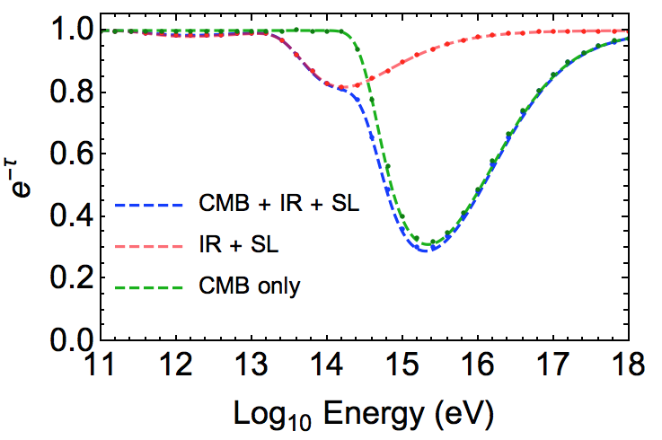
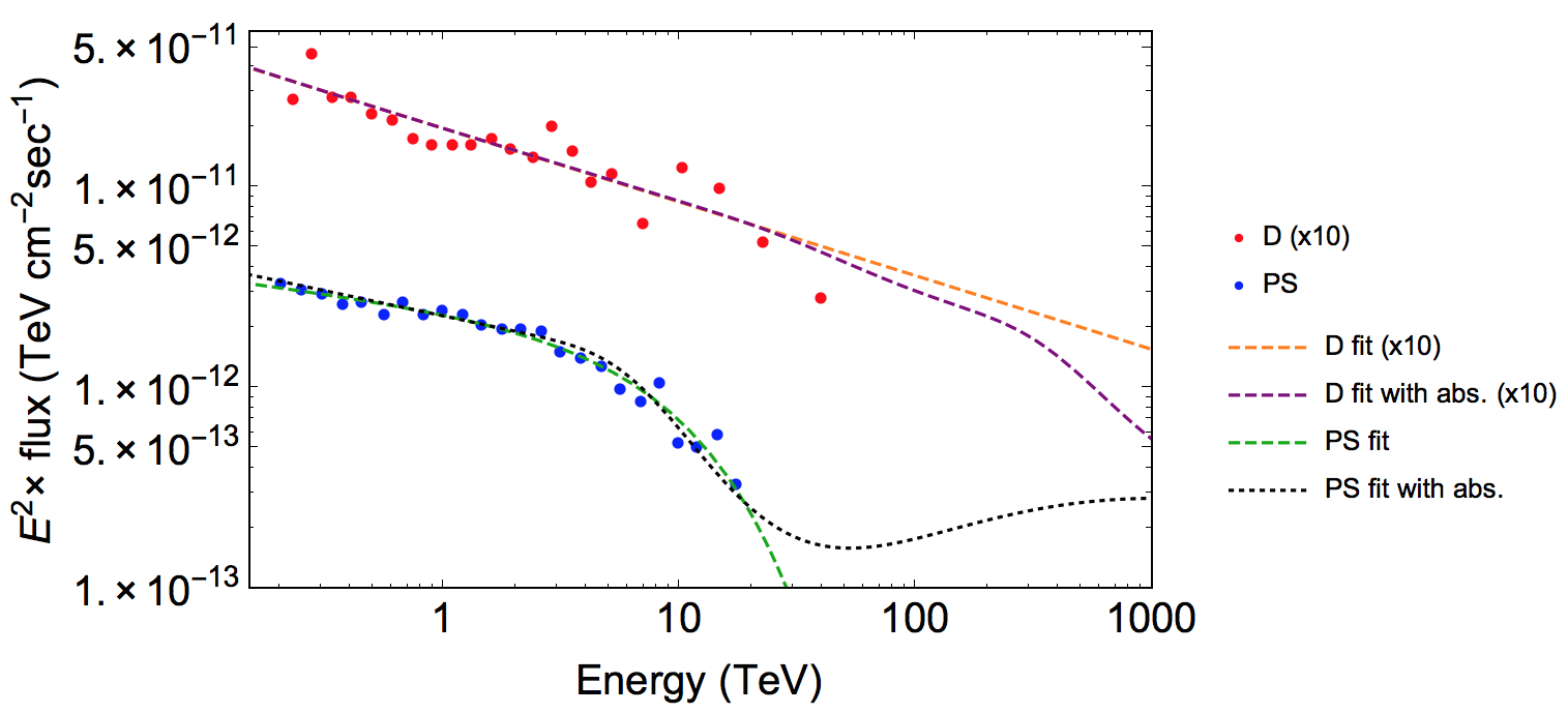
Figure 1: Left panel: Absorption of $\gamma$-rays from the Galactic Center at different energies, due to the interaction with CMB, IR and SL. Right panel: fits of the H.E.S.S. data. D is the Diffuse flux, PS is the Point Source flux. For D, absorption due to CMB, IR and SL is considered. For PS, an increased absorption, due to non standard radiation field, is considered. As visual aid, in the right panel we indicate the central values of the measurements for the Diffuse and the Point Source by red and blue dots, respectively, as obtained in ref. nature , where uncertainties can also be found.

Formalism

A photon with energy $E_{\gamma}$ emitted from an astrophysical source can interact during its travel to the Earth with ambient photons, producing electron-positron pairs. The probability that it will reach the Earth is

$$P(E_{\gamma})=\exp\left[-\tau(E_{\gamma})\right]$$ (2)

where $\tau$ is the opacity. In the interstellar medium, different radiation fields can offer a target to astrophysical photons and determine their absorption: the total opacity is therefore the sum of various contributions,

$$\tau=\sum_{i}\tau_{i}$$ (3)

where the index $i$ indicates the components of the background radiation field that causes absorption. These include the CMB, as well as the IR and SL backgrounds, and possibly new ones, present near the region of the Galactic Center.

Table 1: Values of the parameters of the background radiation fields used for the computation of the absorption factor of the $\gamma$-rays from the Galactic Center: the black body temperature $T_{i}$, the non-thermic parameter $\xi_{i}$, the typical length $L_{i}$ (namely the distance of the Galactic Center for CMB and the exponential scales for the IR and SL radiation fields) the total density of photons $n_{\gamma,i}$ (obtained from Eq. 6), the typical energy $E_{i}$ (obtained from Eq. 7).

Rad. field	$T_{i}$	$\xi_{i}$	$L_{i}$	$n_{\gamma,i}$	$E_{i}$
	(eV)		(kpc)	(cm-3)	(TeV)
CMB	$2.35\cdot 10^{-4}$	1	8.3	410.7	1111
IR	$3.10\cdot 10^{-3}$	$1.55\cdot 10^{-4}$	4.1	146.0	84.23
SL	$3.44\cdot 10^{-1}$	$1.47\cdot 10^{-11}$	2.4	19.0	0.26

For a thermal distribution (or for a distribution proportional to a thermal distribution) the opacity from the $i$-th component is given simply by

$$\tau_{i}(E_{\gamma})=1.315\times\frac{L_{i}}{L_{0}}\times\frac{n_{\gamma,i}}{n_{\gamma,\mbox{\tiny CMB}}}\times f\!\left(\frac{E_{i}}{E_{\gamma}}\right)$$ (4)

where the quantities chosen for the normalization are $L_{0}$=10 kpc (a typical galactic distance) and $n_{\gamma,\mbox{\tiny CMB}}=\rm 410.7\ cm^{-3}$. The various quantities in this formula are discussed in details below, the numerical values (adopted in the calculation) are given in Tab. 1. The overall figure gathers few constants from the thermal CMB distribution, from the interaction cross section, and the distance $L_{0}$. Its expression is

$$\frac{\pi}{2\ \zeta(3)}\times\displaystyle L_{0}\>r_{e}^{2}\times n_{\gamma,\mbox{\tiny CMB}}=1.315$$ (5)

where $r_{e}=e^{2}/(m_{e}c^{2})\approx 2.818\times 10^{-13}$ cm is the classical electron radius and $\zeta(3)\approx 1.20206$ the Riemann’s zeta function. Here we examine and discuss the various quantities appearing in Eq. 4.
i) The parameter $L_{i}$ is the size of the background radiation field. In the case of the CMB, this is just the distance between the Galactic Center and the detector (i.e., 8.3 kpc) because the CMB is uniformly distributed throughout the interstellar medium. The IR and SL radiation fields, instead, obey an approximate exponential distribution from the Galactic Center. The density of photon is, ${n_{\gamma,i}}(L)={n_{\gamma,i}}\,e^{-L/L_{i}}$. Thus, the product ${n_{\gamma,i}}\times L_{i}$ is the column density of photons, and also for the IR and SL fields (as for the CMB) $L_{i}$ represents the effective size of the region where the radiation is present. The values of the scales $L_{i}$ are given in Tab. 1.
ii) $n_{\gamma,i}$ is the total number of photons of the considered background radiation field. Comparing IR and SL with the CMB we found that the total number of photons, in the first two cases, are given by the following expression:

$$n_{\gamma,i}(\xi_{i},T_{i})=\xi_{i}\times n_{\gamma,\mbox{\tiny CMB}}\times\left(\frac{T_{i}}{T_{\mbox{\tiny CMB}}}\right)^{3}$$ (6)

where $\xi_{i}\leq 1$ is a numerical factor, the non-thermic parameter, chosen to reproduce the observed distribution of ambient photons (the case $\xi_{i}=1$ is the thermal one).
iii) The energy $E_{i}$ is linked to the black body (or quasi black body for IR and SL) temperature $T_{i}$, through the relation

$$E_{i}(T_{i})=\frac{m_{e}^{2}}{T_{i}}$$ (7)

where $m_{e}$ is the electron mass and the assumed distribution is proportional to a thermal distribution with temperature $T_{i}$.
iv) The adimensional function $f(x)$, where $x=\frac{E_{i}}{E_{\gamma}}$, describes how the absorption varies with the energy of the $\gamma$-ray. It was first obtained in Ref. moska using the results of breit . This is discussed in the appendix, where precise values are obtained by means of numerical calculation. We derived a simple approximated expression for such a function,

$$f(x)\simeq-a\cdot x\cdot\log[1-\exp(-b\ x^{c})],\ \ \ \left\{\begin{array}[]{l}a=3.68\\ b=1.52\\ c=0.89\end{array}\right.$$ (8)

which is very easy to use and accurate to within 3%.

The values of $T_{i}$, $\xi_{i}$ and $L_{i}$ for the known components were found fitting the energy spectra of radiation reported in GALPROP (Ref. galprop ). They are summarized in Tab. 1 for the CMB, IR and SL radiation fields from the Galactic Center to the Earth. The latter two contributions affect the survival probability at energies smaller than those due to the CMB photons. The parameters $n_{\gamma,i}$ and $E_{i}$ are also given in table Tab. 1, to allow one to use directly of Eq. (4) just replacing the appropriate numerical values. In this formalism, a population of quasi-thermal background photons is characterized by the parameters $T_{i},\xi_{i},L_{i}$, and it will yield the opacity factor $\tau_{i}=\tau(E_{\gamma};T_{i},\xi_{i}\times L_{i})$. Note that $\xi_{i}$ and $L_{i}$ appear in Eq. 4 only through their product, so for each component of the background radiation field (known or hypothetical) we have a two parameter description of photon absorption.

Results

The effects of absorption due to the known radiation fields of Tab. 1, that concern the $\gamma$-rays propagating from the Galactic Center to the Earth, are illustrated in the left panel of Fig. 1. They become relevant at some hundreds of TeV, so the $\gamma$-rays presently observed by H.E.S.S. from the Diffuse region (and the models D and DC introduced above) are not significantly influenced by this phenomenon, assuming only the radiation fields Porter:2008ve used in GALPROP. Therefore it is possible to use directly the observed diffuse $\gamma$-ray flux in order to obtain the $\gamma$-ray flux at the source, modulo the caveats concerning the extrapolation at high energy, see Sect. II.

On the other side, the flux from the Point Source could be affected by the absorption due to a new, non standard and intense radiation field close to the central black-hole. In fact, the physical conditions in the close vicinity of the supermassive black-hole are not perfectly known and in particular the local radiation field is not probed directly. Recall that the $\gamma$-ray spectrum from the Point Source observed by H.E.S.S. deviates from a power law distribution at the higher energies currently probed: it would naturally differ from the emitted $\gamma$-ray spectrum in presence of a new radiation field. In particular, the cut-off of the emitted spectrum would move towards higher energies.

We show below that, hypothesizing a significant absorption of $\gamma$-rays close to the black-hole, the flux emitted from the Point Source is compatible with a power law distribution at the energies observed by H.E.S.S. and above, just as the one due to the Diffuse $\gamma$-ray component. This speculative scenario allows us to estimate in a reasonable way the maximum effect of absorption due to yet unknown radiation fields. Note that this has a direct implication on the neutrino signal, that we quantify later on.

In this scenario, the background radiation field that causes absorption is characterized by a temperature $T=1.3\times 10^{-2}$ eV, namely, should be in the far infrared spectral band. Hypothesizing a black body field, the corresponding density of photons is equal to $n^{\mbox{\tiny max}}_{\gamma}=7.04\times 10^{7}\ \rm cm^{-3}$, with a typical scale of the radiation field of $L_{\mbox{\tiny min}}=0.07\rm\ pc$, namely with a column density corresponding to $L\times n_{\gamma}\simeq 5000\ \rm\textrm{kpc cm}^{-3}$. If the radiation field is not exactly thermal, the number density of photons decreases whereas the typical length increases: for example, with a non-thermic parameter $\xi=0.02$, we obtain $n_{\gamma}=1.4\times 10^{6}\ \rm\textrm{cm}^{-3}$ and a typical length $L=3.5\ \rm pc$.

This is illustrated in the right panel of Fig. 1. The curve called “PS fit with non standard abs.” is a power law spectrum with the same spectral index and normalization of the PS model of Sect. II, that is modified taking into account the above scenario for $\gamma$-ray absorption.

Some remarks on this scenario are in order:
1) Such non standard IR radiation field could be produced in the reprocessing of the radiation from the central source, due to collision with CircumNuclear Disk clumps, as reported in Ref. smbh .
2) Evidently, the Diffuse component would be not affected by this new IR radiation, because it is far enough from the Galactic Center.
3) As one understands from Fig. 1, if one wants to determine observationally whether the cut-off is intrinsic to the source or it is an absorption feature, measurements of $\gamma$-rays at energies above tens of TeV are required: indeed, the absorption results in a peculiar distortion of the power-law spectrum, that is expected to be different from the effect of an exponential cut-off above $\sim$50 TeV. This discrimination should be possible with CTA cta or with other future instruments.

IV High-energy neutrinos from the Galactic Center Region

Neutrinos could be produced in hadronic interactions of PeV protons with the ambient gas: since each neutrino carries about 5% of the energy of the parent proton, we expect to see neutrinos in the multi-TeV range, in angular correlation with the high-energy $\gamma$-rays emitted from the Galactic Center Region. This scenario is supported by the observed correlation between the $\gamma$-ray emission and molecular clouds reported in nature .

Present upper limit on neutrinos from Sgr A*

To date, IceCube has set the best 90% C.L. upper limit on the $\nu_{\mu}+\mathrm{bar}{\nu}_{\mu}$ flux assuming an unbroken E^-2 spectrum from Sgr A* at icnew ,

$$\phi_{\nu_{\mu}}+\phi_{\mathrm{bar}{\nu}_{\mu}}=7.6\times 10^{-12}\left(\frac{E}{\mbox{TeV}}\right)^{-2}\mbox{ TeV${}^{-1}$ cm${}^{-2}$ s${}^{-1}$}$$ (9)

Such a limit corresponds to the absence of a significant event excess over the known background, that in the analysis of IceCube baka amounts to 25.2 background events in a circle of $1^{\circ}$. This limit has been obtained by means of downward-going track-type events, as discussed in the next section.

Presumably, this is the safest information we have on the neutrino emission from Sgr A*, even if it does not correspond to a realistic assumption on the emitted neutrino spectrum. In principle, the assumption of a differential neutrino spectrum in the form of an E^-2 dependence would be a consequence of the first order Fermi acceleration mechanism, but there is no observational evidence that this is a reliable assumption, and moreover, this is not supported by the observed $\gamma$-ray spectrum.

Model prediction / theoretical upper bound

The model prediction that we are going to derive is based instead on the current $\gamma$-ray observations and on the assumption that such emission is fully hadronic. The expectation that we obtain is well compatible with the IceCube non-detection. Indeed, the flux of Eq. 9 is much larger and has a distribution harder than the upper limit on the neutrino flux derived from the $\gamma$-ray observations. This is evident from Fig. 2, discussed in details just below.

Keeping in mind the crucial hypothesis, that the $\gamma$-rays observed by H.E.S.S. are fully hadronic, our model prediction can be regarded also as a theoretical upper bound. It is very important however to distinguish clearly the experimental upper limit of Eq. 9 from this theoretical upper limit on the expected neutrino signal, derived through $\gamma$-rays. The latter is more realistic and also much more stringent, but, just as the former, it depends upon various theoretical assumptions.

In order to illustrate this point, we remark that the $\gamma$-ray data collected by H.E.S.S. cannot exclude that the $\nu_{\mu}+\mathrm{bar}\nu_{\mu}$ spectrum hardens to E^-2 above 20-40 TeV; however, the normalization of this component has to be some 5 times smaller than Eq. 9, if the spectrum is a smooth distribution (a continuous function) linked to the observed $\gamma$-rays spectrum. This kind of (very speculative) scenario, along with other scenarios mentioned in Sect. II, might increase the expected neutrino signal.

However, below in this work, we prefer to focus conservatively on the minimal scenario that was defined in Sect. II as it is motivated by H.E.S.S. measurements. We will show that the theoretical limit on the neutrino flux, corresponding to the $\gamma$-ray flux observed by H.E.S.S., is below the capabilities of the detectors currently in data-taking, whereas it could be within the reach of the future detectors.

Method to calculate the muon neutrino flux

Assuming a purely hadronic origin of the emission $\gamma$-ray spectrum $\phi_{\gamma}(E)$, we can calculate the muon neutrino and antineutrino spectrum through the precise relations based on the assumption of cosmic ray-gas collisions villantevissani ,

$$\begin{array}[]{rl}\phi_{\stackrel{{\scriptstyle(-)}}{{\nu}}_{\!\!\mu}}(E)&\displaystyle=\alpha_{\pi}\ \phi_{\gamma}\left(\displaystyle\frac{E}{1-r_{\pi}}\right)+\alpha_{K}\ \phi_{\gamma}\left(\displaystyle\frac{E}{1-r_{K}}\right)+\\ &\displaystyle+\int_{0}^{1}{\frac{dx}{x}\ K_{\stackrel{{\scriptstyle(-)}}{{\nu}}_{\!\!\mu}}(x)\ \phi_{\gamma}\!\left(\frac{E}{x}\right)}\end{array}$$ (10)

where $\alpha_{\pi}=0.380\ (0.278)$ and $\alpha_{K}=0.013\ (0.009)$ for $\nu_{\mu}$ and $\mathrm{bar}\nu_{\mu}$ respectively and where $r_{x}=(m_{\mu}/m_{x})^{2}$ with $x=\pi,K$. In each expression, the first two contributions describe neutrinos from the two-body decay by pions and kaons, while the third term accounts for neutrinos from muon decay. The kernels for muon neutrinos $K_{\nu_{\mu}}(x)$ and for muon antineutrinos $K_{\mathrm{bar}{\nu}_{\mu}}(x)$, which also account for oscillations from the source to the Earth, are

$$\footnotesize{K_{\nu_{\mu}}(x)\!=\!\left\{\begin{array}[]{ll}x^{2}(15.34-28.93x)&0<x\leq r_{K}\\ 0.0165+0.1193x+3.747x^{2}-3.981x^{3}&r_{K}<x<r_{\pi}\\ (1-x)^{2}(-0.6698+6.588x)&r_{\pi}\leq x<1\\ \end{array}\right.}$$

$$\footnotesize{K_{\mathrm{bar}{\nu}_{\mu}}(x)\!=\!\left\{\begin{array}[]{ll}x^{2}(18.48-25.33x)&0<x\leq r_{K}\\ 0.0251+0.0826x+3.697x^{2}-3.548x^{3}&r_{K}<x<r_{\pi}\\ (1-x)^{2}(0.0351+5.864x)&r_{\pi}\leq x<1\\ \end{array}\right.}$$

Applying such procedure, the expected (upper limits on the) neutrino spectra are obtained from the $\gamma$-ray spectrum. This is the closest we can go to a model-independent approach.

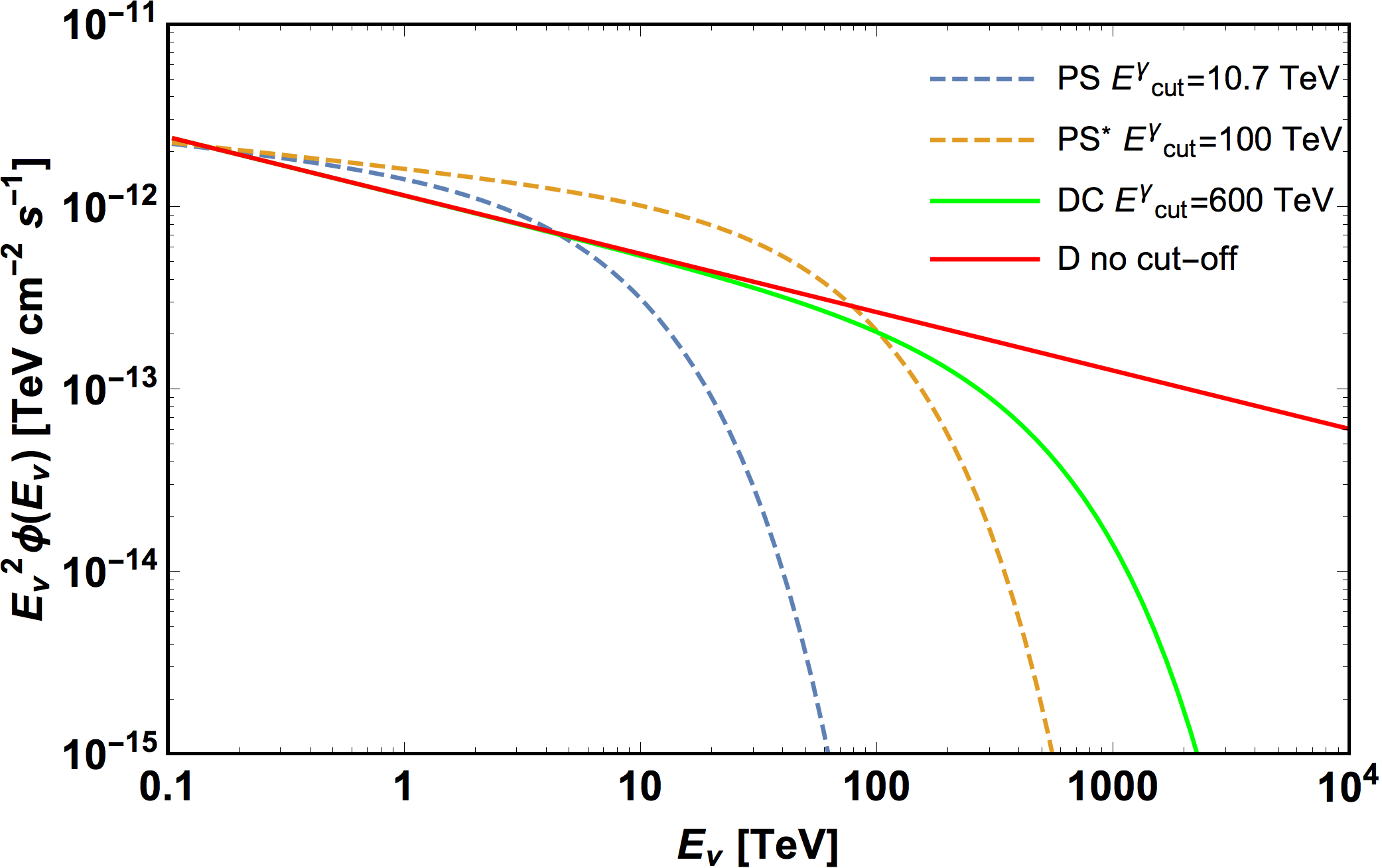
Figure 2: Predicted muon neutrino and antineutrino fluxes (summed) for the Point Source best fit with a cut-off at E${}^{\gamma}_{\textrm{\tiny cut}}=10.7$ TeV and for an arbitrary cut-off at E${}^{\gamma}_{\textrm{\tiny cut}}=100$ TeV. Also shown the fluxes for the Diffuse best fit without cut-off and with a cut-off at E${}^{\gamma}_{\textrm{\tiny cut}}=600$ TeV.

Results for the $\nu_{\mu}+\mathrm{bar}\nu_{\mu}$ fluxes

We show in Fig. 2 the sum of the muon neutrino and antineutrino fluxes, derived using for $\phi_{\gamma}(E)$ the four models introduced in Sect. II, namely: 1) the best fit flux of the Point Source region (with 10.7 TeV cut-off), 2) the same one assuming that the cut-off is at 100 TeV, 3) the best fit flux of the Diffuse region (without cut-off), 4) the same one including a cut-off at 600 TeV.
Our results compare reasonably well with the fluxes given in the Extended Data Figure 3 of ref. nature , that however concern the total flux of neutrinos (i.e., all three flavors). The conclusion stated in Ref. nature , based on the observed $\gamma$-ray fluxes and on the criterion stated in vissanga , is that these fluxes are potentially observable.
Here, we would like to proceed in the discussion further, clarifying the condition for observability in the existing detectors and quantifying the expected number of signal events that can be detected. We will discuss how the conclusion depends upon the features of the detector.

V Expected signal in neutrino telescopes

Current neutrino telescopes, like ANTARES antares , IceCube icecube and those under construction as KM3NeT arca and Baikal-GVD gvd , could be able to detect the neutrinos from the Galactic Center Region by looking for track-like events from the direction of this source.

Track-like signal events and background events

The use of track-like events for the search of point sources is desirable because of the relatively good angular resolution, of the order of $1^{\circ}$ in ice and several times better in water. This allows the detectors to operate with a manageable rate of background events, due to atmospheric muons and neutrinos.

The atmospheric neutrinos are an irreducible source of background events for all detectors. They can be discriminated from the signal of a point source due to the fact that they do not have a preferential direction, and moreover they have a softer energy spectrum than the one expected from the Galactic Center Region. Part of the atmospheric neutrinos from above can be identified and excluded thanks to the accompanying muons, for neutrino energies above 10 TeV and zenith angles less than $60^{\circ}$ according to schonert . This rejection method works for the search of High-Energy Starting Events (HESE) above 30 TeV in IceCube, since it removes 70% of atmospheric neutrinos in the Southern Hemisphere icescience . Its application in our case is less effective. The first reason is obvious: Sgr A* is observed at a high zenith angle from the South Pole, $\theta_{Z}=90^{\circ}-29^{\circ}=61^{\circ}$. Moreover, an important fraction of the signal is below 10 TeV, as discussed later in this section.

For what concerns atmospheric muons, one should distinguish, broadly speaking, the cases when the track-type events of interest for the search of the signal are upward-going or downward-going:
1) The first class of events is not subject to the contamination of atmospheric muons. Due to the position of Sgr A*, this kind of events can be observed by detectors located in the Northern hemisphere.
2) The second class of events is subject to the contamination of atmospheric muons. Due to the position of Sgr A*, this is relevant for IceCube. IceCube has successfully exploited a subset of downward-going track events with the purpose of investigating neutrino emission from Sgr A* effI , by requiring the additional condition that the production vertex of the downward-going tracks is contained in the detector.

To be precise, the fraction of time when the source is below the horizon is given by the expression $f_{\mbox{\tiny below}}=1-{\mbox{Re}[\arccos(-\tan\delta\tan\varphi)]}/{\pi}$ exa . Its value is

$$f_{\mbox{\tiny below}}=0\%,64\%,68\%,76\%$$ (11)

for IceCube, KM3NeT-ARCA, ANTARES and GVD respectively, where the declination of the Galactic Center is equal to $\delta$(Sgr A*)=-29.01^∘ and where the latitudes North of the various detectors are $\varphi=-90^{\circ},36.27^{\circ},42.79^{\circ},51.83^{\circ}$ for IceCube, KM3NeT-ARCA, ANTARES and GVD respectively. In this fraction of time, the atmospheric muon background is suppressed and the search for a signal is easier.

The search for a signal with upward-going tracks allows one to increase the effective volume of neutrino detection to the surrounding region, where the produced muon reaches the detector with sufficient energy. Also the condition that the vertex is contained reduces the atmospheric muon background greatly, even in the low-energy region where it is more abundant. However, this condition does not allow to use the full volume of the detector but only a part of it, which hinders the search for a signal, especially a weak signal as the one we are discussing.

Another specific circumstance favors the Cherenkov telescopes operated in water, in comparison to those operated in ice, in the search for a neutrino signal at low energies. This is due to the angular resolution $\delta\theta$, that is better (i.e., smaller) in water than in ice. The number of background events $b$, falling in a given search window, decreases as $\delta\theta^{2}$; the observable signal $s$ depends upon $s/\sqrt{b}$, that scales as $1/\delta\theta$. In any detector, there is a minimum energy below which the search for a signal becomes very challenging, since the number of background events tends to be excessively large. In water based detectors, this energy is smaller than in the case of ice based detectors, simply because the number of background events decreases with angular resolution. For this reason, the neutrino telescopes operated in water are more sensitive than the telescopes operated in ice, and can afford to use smaller energy threshold for data taking.

The IceCube upper limit mentioned in Sect. IV is based on downgoing tracks and of course this telescope is operated in ice. We will show in the next paragraph that the use of a water based telescopes in the Northern hemisphere, able of good performances at low energies, can achieve significantly better results and have even the potential to probe the predictions of our model.

In principle, IceCube can also look at the Southern sky by exploiting the HESE sample icecube , namely events of high energy with a vertex contained in the detector. The HESE are mainly composed of shower-type events, that have an angular uncertainty of about $10^{\circ}$, much worse than that of track-like events. Recall that IceCube used this data set to discover a population of diffuse (= unidentified) neutrino sources. The HESE sample was obtained adopting a very high energy threshold ($\sim 30$ TeV): this warrants a sufficiently clean sample, but requires a rather intense flux to produce an observable signal. However, in the case of Sgr A* we are interested in a point-source and to lower energy, so a high angular precision on the reconstructed event direction and an energy threshold much lower than 30 TeV are needed. We will show the importance of these considerations by a direct quantitative evaluation of the HESE event rate.

Effective areas

The angular resolution for current neutrino telescopes is such that both the PS and the D regions are seen as point-like regions. Thus, the effective areas of ANTARES effA and IceCube effI are those used for the search of point-like sources in the declination range relevant for the observation of the Galactic Center. Likewise, the effective area of KM3NeT-ARCA effK refers to the point source search: it is applied to the next configuration including two building blocks, each with 115 detection units. These effective areas, that we use for the calculation of the rates, are shown in Fig. 3.

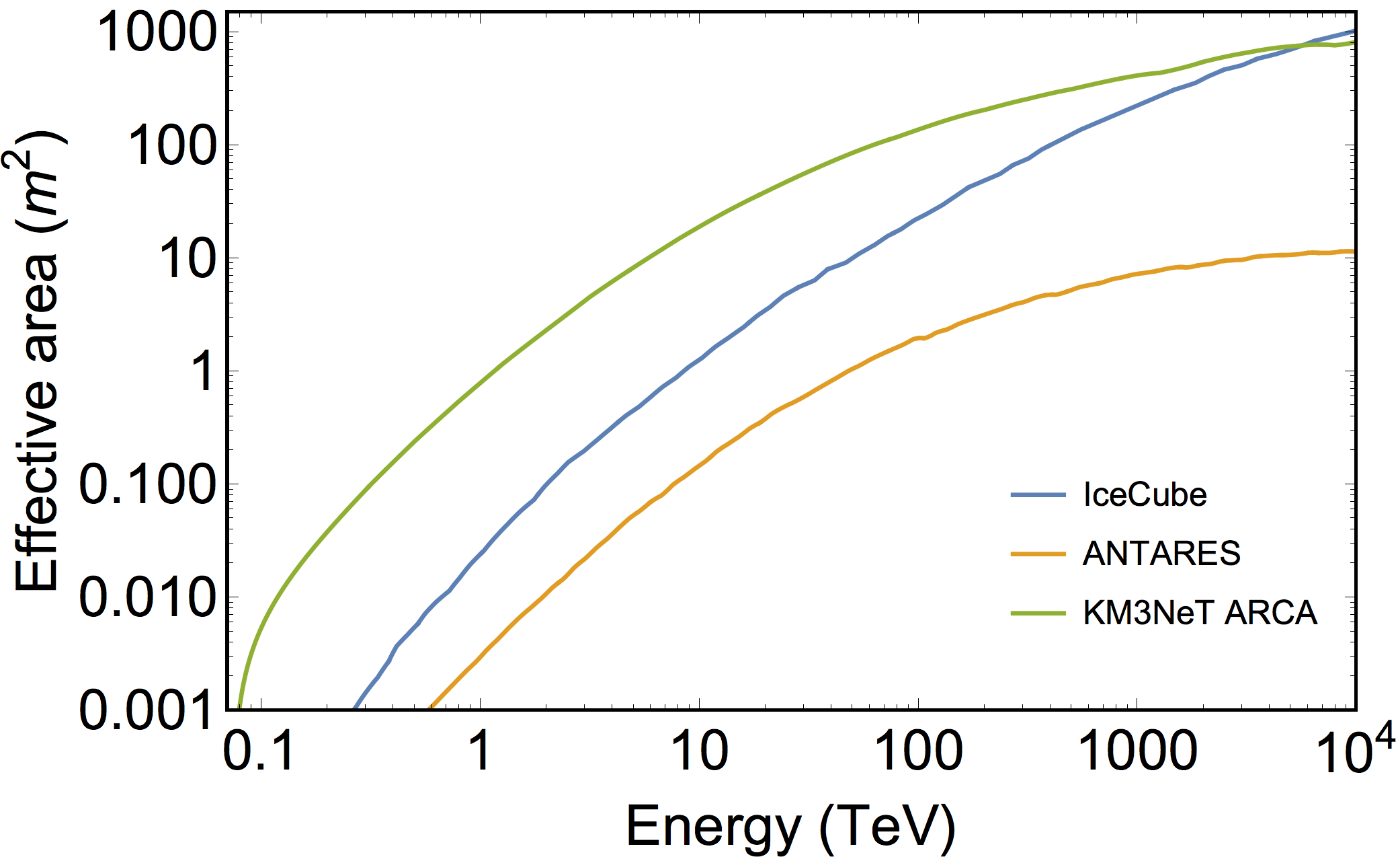
Figure 3: Muon neutrino effective areas for point-source search adopted in the calculation. The one adopted for ANTARES is that in the declination band $-45^{\circ}<\delta<0^{\circ}$, the one for IceCube is for $-30^{\circ}<\delta<0^{\circ}$, the one for ARCA is an average value. See the text for references and for discussion.

The rate of events that a detector is able to measure, assuming a certain angular search region, is given by the convolution of the expected flux from the source, $\phi_{\nu_{\mu}}(E)+\phi_{\mathrm{bar}{\nu}_{\mu}}(E)$, and the detector effective area, $A_{\textrm{\tiny eff}}(E)$, through the relation,

$$\textrm{R}=\int{[\phi_{\nu_{\mu}}(E)+\phi_{\mathrm{bar}{\nu}_{\mu}}(E)]\,A_{\textrm{\tiny eff}}(E)\,dE}$$ (12)

The integrand in this formula, namely the product of the neutrino fluxes and of the effective areas, is the distribution of parent neutrino energies. Therefore, using the neutrino fluxes of Fig. 2, we can evaluate the neutrino energies that contribute to the point source (PS) signal for IceCube, ANTARES and KM3NeT-ARCA. The results are reported in Fig. 4 and in Tab. 2. This proves that the signal expected from Sgr A* is at relatively low energies.

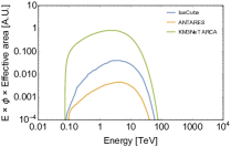
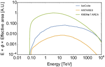
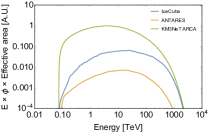
Figure 4: Parental neutrino energies of the signal in arbitrary units. From left to right the Point Source case (PS), the Diffuse case (D) and the Diffuse with a cut-off at E${}^{\gamma}_{\textrm{\tiny cut}}=600$ TeV (DC). See also Tab. 2.

Table 2: Here reported are the median energy E_50% of the parental distribution and energy interval $[$E${}_{\tiny{16\%}}-$E${}_{\tiny{84\%}}]$ where 68% of the signal is expected to be detected for the same models considered in Fig. 4: the Point Source flux (PS), the Diffuse flux (D) and the Diffuse flux with Cut-off at E${}^{\gamma}_{\tiny{cut}}=600$ TeV (DC). All energies are given in TeV.

		ANTARES			ARCA			IceCube
	E50%	E16%	E84%	E50%	E16%	E84%	E50%	E16%	E84%
PS	3.3	1.0	9.2	3.4	1.1	9.2	1.9	0.5	6.3
D	21.9	2.8	179.1	15.0	2.6	89.2	4.8	0.8	34.4
DC	14.8	2.3	88.5	12.1	2.3	60.1	4.3	0.8	26.3

As discussed above, KM3NeT and ANTARES can look at the Galactic Center using upward-going muons, while IceCube has to use downward-going muons further subject to the condition that their vertex is contained in the detector; moreover, the first type of telescopes has a much better angular resolution, which allows them to reduce the background considered in the analysis, thus increasing the signal to noise ratio. Despite the fact that the dimensions of KM3NeT and IceCube are comparable, the effective areas differ significantly at low energies, as can be ascertained from Fig. 3. Note however that the two effective areas become very similar around PeV energies, as expected because of the similar physical sizes of these two neutrino telescopes. The different effective areas lead to the difference in the number of events expected in IceCube and KM3NeT, which amounts to about an order of magnitude.

Remarks

One cautionary remark on KM3NeT-ARCA effective area is in order. To the best of our knowledge, Ref. effK is the only public source of an effective area for point source search with the KM3NeT-ARCA neutrino telescope. We will use it to evaluate the expected signal from the Galactic Center Region, since this is the best that we can do at present, but if one wants to maintain a cautious attitude, one should contemplate the possibility that the experimental cuts adopted and consequently the effective area will change in future releases. As we noted, the existing effective area is quite large, e.g., in comparison to the one of IceCube, but as we demonstrate below, it corresponds to a signal of a few events per year only. Thus, it will be important to know whether the experimental cuts, that will be eventually implemented by the KM3NeT collaboration for the search of the signal, will be compatible with similarly large effective area or will imply its revision.

Finally, we would like to complete the discussion about the reason why IceCube cannot usefully exploit the data set at lower energies. Since the atmospheric neutrino background has a steeper spectrum with respect to the cosmic neutrino spectrum, at low energies it grows more than the signal, and therefore a very stringent selection has to be implemented on data in order to reject such a background. This can be for example realized through a tag: the atmospheric neutrino tag based on the accompanying muons works if the muons reach the detector with sufficient energy. The accompanying muons should have enough energy in the production point to be revealed, which in turn means that the neutrino should have high energy, too. In our case, however, a significant part of the signal is below the lower value of 10 TeV indicated in schonert , as it is shown in Tab. 2. This implies that the efficiency of the atmospheric neutrino tag is less than for the search of HESE above 30 TeV icescience . Recall that Sgr A* is observed at a zenith angle larger than the lower value of $60^{\circ}$ indicated in schonert , and therefore, the accompanying muons lose a significant amount of energy before reaching IceCube. These considerations limit to relatively high energies the region where IceCube may conveniently search for a point source from Sgr A*, as quantified by the effective area reported by the IceCube collaboration.

Table 3: First 4 columns: Spectral parameters assumed for the $\gamma$-ray fluxes, consistent with the H.E.S.S. observations as explained in the text: the search region (PS=Point Source or D=Diffuse), the spectral index $\Gamma$, the flux normalization $\phi_{0}$ in units of 10^-12 TeV^-1 cm^-2 s^-1 and the energy cut-off E${}_{\textrm{\tiny cut}}$ in TeV (see Eq. 1). For the PS and the D models, we show also the maximum and minimum expected values. For the PS* model we assume a scenario with an increased, non standard $\gamma$-ray absorption. Last 4 columns: Expected number of $\nu_{\mu}+\mathrm{bar}\nu_{\mu}$ events per year: downward-going tracks and HESE events in IceCube, upward-going tracks in ANTARES and ARCA. The significant increase of the event rate passing from the PS (1^st row) to the PS* (4^th one) model is linked to the non standard $\gamma$-ray absorption.

		$\!\!\gamma$-rays			$\!\!\!\nu_{\mu}+\mathrm{bar}{\nu}_{\mu}\!\!\!$
	$\Gamma$	$\phi_{0}\!$	E${}_{\textrm{\tiny cut}}\!$	R${}^{\textrm{\tiny ANTARES}}\!\!$	R${}^{\textrm{\tiny ARCA}}\!\!\!$	R${}^{\textrm{\tiny IC}}\!\!$	R${}^{\textrm{\tiny IC}}\!\!_{\textrm{\tiny HESE}}$
PS	2.14	2.55	10.7	$6.2\cdot 10^{-3}$	1.1	$5.2\cdot 10^{-2}$	$1.4\cdot 10^{-6}$
”	2.04	2.92	13.6	$9.5\cdot 10^{-3}$	1.5	$8.2\cdot 10^{-2}$	$6.1\cdot 10^{-6}$
”	2.24	2.18	7.8	$3.9\cdot 10^{-3}$	0.7	$3.2\cdot 10^{-2}$	$1.9\cdot 10^{-7}$
PS*	2.14	2.55	100	$1.7\cdot 10^{-2}$	2.1	$1.5\cdot 10^{-1}$	$5.0\cdot 10^{-4}$
D	2.32	1.92	-	$1.2\cdot 10^{-2}$	1.4	$1.3\cdot 10^{-1}$	$2.2\cdot 10^{-3}$
”	2.20	2.21	-	$2.1\cdot 10^{-2}$	2.2	$2.6\cdot 10^{-1}$	$5.5\cdot 10^{-3}$
”	2.44	1.63	-	$7.5\cdot 10^{-3}$	1.0	$7.4\cdot 10^{-2}$	$8.8\cdot 10^{-4}$
DC	2.32	1.92	400	$1.0\cdot 10^{-2}$	1.3	$9.7\cdot 10^{-2}$	$6.8\cdot 10^{-4}$
DC	2.32	1.92	600	$1.1\cdot 10^{-2}$	1.3	$1.0\cdot 10^{-1}$	$8.8\cdot 10^{-4}$
DC	2.32	1.92	2900	$1.2\cdot 10^{-2}$	1.4	$1.2\cdot 10^{-1}$	$1.6\cdot 10^{-3}$

Expected signal rates

The rates of events for ANTARES, KM3NeT-ARCA and IceCube are given in Tab. 3 with the names $\mbox{R}^{\tiny\mbox{ANTARES}}$, $\mbox{R}^{\tiny\mbox{ARCA}}$, $\mbox{R}^{\tiny\mbox{IC}}$, considering the different spectral model of $\gamma$-ray data presented above, and accounting for both contributions from muon neutrinos and antineutrinos, as expressed in Eq. 10. Baikal-GVD will have a threshold of few TeV and a volume similar to KM3NeT-ARCA, so the results are expected to be similar, but we cannot provide a precise evaluation of the signal since we do not have the effective area.

For comparison, we calculated that the expected rate corresponding to Eq. 9 (namely assuming a E^-2 distribution) in IceCube is 3.8 per year, namely, more than one order of magnitude above the values of Tab. 3. This illustrates the great importance of investigating the $\gamma$-ray distribution at higher energies than currently observed.

As can be seen from Tab. 3, the detectors located in the Northern hemisphere are better suited for neutrino searches from Sgr A*. In fact, when the source is below the horizon, they can observe the Galactic Center Region through upward-going track events, that are not polluted by the atmospheric muons. Such detectors are ANTARES, Baikal-GVD and KM3NeT. We find that the expected rates in ANTARES are just one order of magnitude smaller than those expected in IceCube with downward-going events: this result is well in agreement with the ones in spurio .

For completeness, the rates of the expected HESE track events are also given in Tab. 3. The counting rate is indicated with the name of $\mbox{R}^{\tiny\mbox{IC}}_{\tiny\mbox{\ \ \ HESE}}$ and it was obtained using the effective areas reported in Aartsen:2013jdh . The counting rates are, in the best case, few times $10^{-3}$ HESE events per year. Therefore, this approach does not allow IceCube to search for neutrinos from the Galactic Center.

Discussion

Among the $\gamma$-ray models presented in this table, the most plausible ones are, presumably, those described by a power law with a cut-off.

In the Diffuse case, even considering the less favorable case (the one with lowest energy cut-off, which implies a cut off in the primary spectrum of protons at about 4 PeV, where the knee of the Earth-observed CR spectrum is located) predictions are such that the incoming km³ class detectors in the Northern hemisphere as KM3NeT-ARCA could measure these neutrinos with a rate of few events per year: several years of data-taking will be in any case needed in order to establish the presence of a proton galactic accelerator up to PeV energies and address the origin of very-high-energy cosmic rays. In case of non-detection, however, strong constraints will be derived concerning the proton acceleration efficiency of this poorly-understood source.

A similar conclusion holds true for the Point Source case. When we assume that the cut-off measured by H.E.S.S. is due to the absorption by a non standard background radiation field, the muon neutrino signal increases. E.g., comparing the first row (PS case) and the fourth one (PS*) of Tab. 3 we see an increase by 40-50%; note that the parameter of the exponential cut-off has been set to 100 TeV in the PS* case. Remarkably, the protons accelerated in the source can reach energies up to the PeV scale in this scenario.

Unfortunately, with the current neutrino telescopes, these predictions cannot be probed yet. Anyway, since most of the signal is expected in the 1-100 TeV energy band, the Northern hemisphere telescopes cannot escape from the issue of atmospheric neutrino background events.

VI Conclusions

The recent measurements of multi-TeV $\gamma$-rays from the Galactic Center, performed by H.E.S.S., point out the chance of observing also very-high-energy neutrinos from this part of the Galaxy. The detection of such neutrinos is crucial to confirm or discard the hadronic origin of these $\gamma$-rays. In case of non-detection, however, neutrino telescope will be able to put severe constraints on the efficiency of hadronic acceleration in this source.

In order to estimate the neutrino flux, it is necessary to know the flux of $\gamma$-rays at the source, and for this reason it is crucial to evaluate correctly the effect of the absorption due to the interaction between $\gamma$-rays and the background radiation fields. We have argued that the Diffuse high-energy $\gamma$-ray flux measured by H.E.S.S. is not affected by the absorption. On the contrary, the $\gamma$-ray flux from the Point Source could be affected by an intense infrared radiation field that, if it exists, should be present close to the Galactic Center. We have found that this effect is compatible with an unbroken power law distribution and can increase the observable neutrino signal by 40-50%. This new hypothesis motivates further studies with IR telescopes and with 100 TeV $\gamma$-ray instruments, as the future Cherenkov Telescope Array cta .

We have obtained a precise upper limit on the expected neutrino flux from the regions close to the Galactic Center, assuming that the $\gamma$-rays recently observed by H.E.S.S. are produced by cosmic ray collisions. As shown in Tab. 3, the corresponding maximum signal is of few track (muon signal) events per year in the incoming KM3NeT detector. In view of these results, we conclude that the KM3NeT detector has the best chances to observe neutrinos from Sgr A*, even if, in order to accumulate a large sample of signal events, several years of exposure will be necessary. Besides the analyses of the track-like events in KM3NeT, discussed above, also the analyses of shower-like events will contribute to advance the study of Sgr A*, thanks to the favorable location of this detector and to its superior angular resolution. On the contrary the expected signal in IceCube is smaller and unlikely to be observed in view of the larger background rate caused by the atmospheric muons.

We have examined the reasons of uncertainties in the expectations for the high-energy neutrinos. While a leptonic component of the $\gamma$-ray would decrease the observable signal, several other reasons could increase it, including: the possibility of $\gamma$-ray absorption, an extended angular region around the Galactic Center where the emission is sizeable, a speculative E^-2 behavior of the spectra at higher energies than presently measured with $\gamma$-rays. These considerations emphasize the importance of extending the programs of search and study of high-energy $\gamma$-rays and neutrinos.

VII Acknowledgments

We thank F. Aharonian, S. Gabici, F. Fiore, A. Lamastra and F. Tavecchio for precious discussions. After this study was concluded, two other investigations of $\gamma$-ray absorption appeared: Ref. guo draws a similar picture concerning non standard absorption, Ref. pl focusses on standard effects instead, and our Fig. 1 and their figure 12 are in perfect agreement.

Appendix A Study of the function $f(x)$

The evaluation of the effects of absorption via Eq. (4) rests on the estimation of the properties of the background radiation field and on the calculation of a single universal function. Note in passing that, even if we are interested to use these results to $\gamma$-rays emitted from the Galactic Center, the results concerning $\gamma$-ray absorption can be applied to a very large variety of cases and situations.

In this appendix, we study $f(x)$ in details, providing a table of (virtually exact) numerical values for this function and discussing the bases of the approximation given in Eq. (8). The following material is useful to verify our results and to compare with other results in the literature, but has been confined in this appendix, so that it can be skipped by the uninterested Reader.

The pair creation process breit

$$\gamma+\gamma_{\textrm{\tiny bkg}}\longrightarrow e^{+}+e^{-}$$

in the background of thermal photons with temperature $T_{i}$ gives the opacity factor moska ,

$$\tau_{i}=\frac{1}{\pi}\times r_{e}^{2}L_{i}\times T_{i}^{3}\times f\left(\displaystyle\frac{m_{e}^{2}}{T_{i}\ E_{\gamma}}\right)$$

that can be rewritten introducing the thermal photon density $n_{\gamma,i}=2\zeta(3)T_{i}^{3}/\pi^{2}$. The function $f(x)$ is defined as,

$$f(x)=x^{2}\int_{0}^{1}\!d\beta\ R(\beta)\ \psi\left(\frac{x}{1-\beta^{2}}\right)$$ (13)

Here $\beta$ is the velocity of the outgoing electron in the center of mass frame, and the two auxiliary functions are,

$$\begin{array}[]{l}R(\beta)=\displaystyle\frac{2\beta}{(1-\beta^{2})^{2}}\left[(3-\beta^{4})\log\left(\frac{1+\beta}{1-\beta}\right)-2\beta(2-\beta^{2})\right]\\[8.61108pt] \psi(z)=\displaystyle-\log\left(1-e^{-z}\right)\end{array}$$

with $z=x/(1-\beta^{2})$. Solving numerically the integral in Eq. 13 we found the values reported in Tab. 4.

Table 4: Table of values of the function $f(x)$ as given in Eq. 13. In bold, the value of $x$ in which the function reaches the maximum and half of the maximum.

$x$	$f(x)$	$x$	$f(x)$
$10^{-10}$	$7.32\times 10^{-9}$	$10^{-1}$	$6.32\times 10^{-1}$
$10^{-9}$	$6.57\times 10^{-8}$	0.503	1.076
$10^{-8}$	$5.81\times 10^{-7}$	1	$9.07\times 10^{-1}$
$10^{-7}$	$5.05\times 10^{-6}$	1.77	0.538
$10^{-6}$	$4.29\times 10^{-5}$	5	$3.27\times 10^{-2}$
$10^{-5}$	$3.54\times 10^{-4}$	10	$2.92\times 10^{-4}$
$10^{-4}$	$2.78\times 10^{-3}$	20	$1.78\times 10^{-8}$
$10^{-3}$	$2.04\times 10^{-2}$	30	$9.65\times 10^{-13}$
$10^{-2}$	$1.31\times 10^{-1}$	50	$\simeq 0$
0.0756	0.538

First, we examine the behaviour of the integrand in $\beta$. The function $R(\beta)\sim 4\beta^{2}$ if $\beta\rightarrow 0$; on the contrary, when $\beta\rightarrow 1$, it diverges like $R(\beta)\sim-\frac{\log(1-\beta)}{(1-\beta^{2})^{2}}$. The divergence is compensated by the behavior of the function $\psi(\frac{x}{1-\beta^{2}})$, that follows from $\psi(\frac{x}{1-\beta^{2}})=\sum_{n=1}^{\infty}\frac{e^{-n\frac{x}{1-\beta^{2}}}}{n}$ at high values of $\frac{x}{1-\beta^{2}}$. Finally, $\psi(\frac{x}{1-\beta^{2}})\approx-\log\frac{x}{1-\beta^{2}}$ at small values of $\frac{x}{1-\beta^{2}}$.

At this point, we study the behaviour of $f(x)$ in $x$:
For high $x$ we can consider only the first term of the expansion of $\psi(\frac{x}{1-\beta^{2}})$, so the function $f(x)$ is well approximated by: $f(x)\approx x^{2}\times\int_{0}^{1}\ d\beta\ R(\beta)\exp\left(-\frac{x}{1-\beta^{2}}\right)$ within an accuracy of 1% for $x>3$.
For small $x$ the most important contribution to the integral is given when the $R(\beta)$ diverges and the $\psi(\frac{x}{1-\beta^{2}})$ is not exponentially suppressed. This condition is realized when $\beta<\sqrt{1-x}\approx 1-x/2$ and in this region $\psi(\frac{x}{1-\beta^{2}})\approx-\log\frac{x}{1-\beta^{2}}$; for $R(\beta)$ we can use the asymptotic expression, i.e. $R(\beta)\simeq 4\frac{\log\big{(}\frac{2}{1-\beta}\big{)}}{(1-\beta^{2})^{2}}$. The approximation of the function $f(x$) is given by: $f(x)\approx-4x^{2}\int_{0}^{1-x/2}$ $d\beta\frac{\log\big{(}\frac{2}{1-\beta}\big{)}\log\big{(}\frac{x}{1-\beta^{2}}\big{)}}{(1-\beta^{2})^{2}}$. This implies the behavior, $f(x)\approx-3.076\ x\ \log(x)$ to within an accuracy of about 3% in the interval $10^{-10}\leq x\leq 10^{-5}$.

A global analytical approximation of the $f(x)$, that respects the behavior for small and large values of $x$, is given by Eq. 8. Its accuracy is $\sim 3\%$ into the interval $10^{-10}\leq x\leq 10$. When $x>10$ the function rapidly decreases, as we can see also from Tab. 4, where the values are obtained by numerically integrations without any approximation.

References

- (1) F. Aharonian et al. [HESS Collaboration], Nature 531 (2016) 476
- (2) R. Genzel, F. Eisenhauer and S. Gillessen, Rev. Mod. Phys. 82 (2010) 3121
- (3) G. Ponti, M. R. Morris, R. Terrier and A. Goldwurm, Astrophys. Space Sci. Proc. 34 (2013) 331
- (4) K. Koyama, T. Inui, H. Matsumoto and T.G. Tsuru, Publ. Astron. Soc. Jap. 60 (2008) 201
- (5) M. Freitag, P. Amaro-Seoane and V. Kalogera, Astrophys. J. 649 (2006) 91
- (6) M. Su, T. R. Slatyer and D. P. Finkbeiner, Astrophys. J. 724 (2010) 1044
- (7) R. M. Crocker and F. Aharonian, Phys. Rev. Lett. 106 (2011) 101102
- (8) Y. Fujita, S. S. Kimura and K. Murase, Phys. Rev. D 92 no.2 (2015) 023001
- (9) I. Zheleznykh, Int. J. Mod. Phys. A 21S1 (2006) 1 and M. A. Markov, The Neutrino, Dubna, D-1269 (1963)
- (10) M. G. Aartsen et al. [IceCube Collaboration], The Astrophysical Journal Letters, 824, no. 2, L28 (2016)
- (11) M.L. Costantini and F. Vissani, Astropart. Phys. 23, 477 (2005)
- (12) F. Vissani, F. Aharonian and N. Sahakyan, Astropart. Phys. 34 (2011) 778
- (13) R. W. Springer et al. [HAWC Collaboration], Nucl. Part. Phys. Proc. 279-281 (2016) 87-94
- (14) S. Vercellone et al. [CTA Consortium Collaboration], Nucl. Instrum. Meth. A 766 (2014) 73
- (15) T. A. Porter, I. V. Moskalenko, A. W. Strong, E. Orlando and L. Bouchet, Astrophys. J. 682 (2008) 400
- (16) http://galprop.stanford.edu/
- (17) I.V. Moskalenko, T.A. Porter and A.W. Strong, Astrophys. J. 640 (2006) L155
- (18) S. Lee, Phys. Rev. D 58 (1998)
- (19) M. Cirelli and P. Panci, Nucl. Phys. B 821 (2009 399)
- (20) A. Esmaili and P. D. Serpico, JCAP 1510 (2015) 014
- (21) G. Breit and J.A. Wheeler, Phys. Rev. 46 (1934) 1087
- (22) M. Ageron et al. [ANTARES Collaboration], Nucl. Instrum. Meth. A 656 (2011) 11
- (23) M. G. Aartsen et al. [IceCube Collaboration], Astrophys. J. 809 no.1 (2015) 98
- (24) S. Adrian-Martinez et al. [KM3NeT Collaboration], J. Phys. G: Nucl. Part. Phys. 43 (2016) 084001
- (25) A. D. Avrorin et al. [Baikal-GVD Collaboration], EPJ Web of Conferences 116 (2016) 11005
- (26) S. Schonert, T. K. Gaisser, E. Resconi and O. Schulz, Phys. Rev. D 79 (2009) 043009
- (27) M. G. Aartsen et al. [IceCube Collaboration], Science 342 (2013) 1242856
- (28) M. G. Aartsen et al. [IceCube Collaboration], Astrophys. J. 796 no.2 (2014), 109
- (29) M. G. Aartsen et al. [IceCube Collaboration], Astrophys. J. 779, 132 (2013)
- (30) F.L. Villante, F. Vissani, Phys. Rev. D 78 (2008) 103007
- (31) S. Adrian-Martinez et al. [ANTARES Collaboration], Astrophys. J. 760 (2012) 53
- (32) http://www.ecap.nat.uni-erlangen.de/members/schmid/Doktorarbeit/JuliaSchmidDissertation.pdf
- (33) M. Spurio, Phys. Rev. D 90, no.10 (2014) 103004
- (34) http://icecube.wisc.edu/science/data
- (35) Y. Q. Guo, Z. Tian, Z. Wang, H. J. Li and T. L. Chen, arXiv:1604.08301
- (36) S. Vernetto and P. Lipari, arXiv:1608.01587