I/O-Efficient Generation of Massive Graphs
Following the LFR Benchmark

Abstract

LFR is a popular benchmark graph generator used to evaluate community detection algorithms. We present EM-LFR, the first external memory algorithm able to generate massive complex networks following the LFR benchmark. Its most expensive component is the generation of random graphs with prescribed degree sequences which can be divided into two steps: the graphs are first materialized deterministically using the Havel-Hakimi algorithm, and then randomized. Our main contributions are EM-HH and EM-ES, two I/O-efficient external memory algorithms for these two steps. We also propose EM-CM/ES, an alternative sampling scheme using the Configuration Model and rewiring steps to obtain a random simple graph. In an experimental evaluation we demonstrate their performance; our implementation is able to handle graphs with more than 37 billion edges on a single machine, is competitive with a massive parallel distributed algorithm, and is faster than a state-of-the-art internal memory implementation even on instances fitting in main memory. EM-LFR’s implementation is capable of generating large graph instances orders of magnitude faster than the original implementation. We give evidence that both implementations yield graphs with matching properties by applying clustering algorithms to generated instances. Similarly, we analyse the evolution of graph properties as EM-ES is executed on networks obtained with EM-CM/ES and find that the alternative approach can accelerate the sampling process.

1 Introduction

Complex networks, such as web graphs or social networks, are usually composed of communities, also called clusters, that are internally dense but externally sparsely connected. Finding these clusters, which can be disjoint or overlapping, is a common task in network analysis. A large number of algorithms trying to find meaningful clusters have been proposed (see [16, 22, 17] for an overview). Commonly synthetic benchmarks are used to evaluate and compare these clustering algorithms, since for most real-world networks it is unknown which communities they contain and which of them are actually detectable through structure [4, 17]. In the last years, the LFR benchmark [28, 27] has become a standard benchmark for such experimental studies, both for disjoint and for overlapping communities [14].

With the emergence of massive networks that cannot be handled in the main memory of a single computer, new clustering schemes have been proposed for advanced models of computation [9, 49]. Since such algorithms typically use hierarchical input representations, quality results of small benchmarks may not be generalizable to larger instances. To produce such large instances exceeding main memory, we propose a generator in the external memory (EM) model of computation that follows the LFR benchmark.

The distributed CKB benchmark [11] is a step in a similar direction, however, it considers only overlapping clusters and uses a different model of communities. In contrast, our approach is a direct realization of the established LFR benchmark and supports both disjoint and overlapping clusters.

1.1 Random Graphs from a prescribed Degree Sequence

In preliminary experiments, we identified the generation of random graphs with prescribed degree sequence as the main issue when transferring the LFR benchmark into an EM setting — both in terms of algorithmic complexity and runtime. To do so, the LFR benchmark uses the fixed degree sequence model (FDSM), also known as edge-switching Markov-chain algorithm (e.g. [35]). It consists of a) generating a deterministic graph from a prescribed degree sequence and b) randomizing this graph using random edge switches. For each edge switch, two edges are chosen uniformly at random and two of the endpoints are swapped if the resulting graph is still simple (for details, see section 5). Each edge switch can be seen as a transition in a Markov chain. This Markov chain is irreducible [13], symmetric and aperiodic [18] and therefore converges to the uniform distribution. It also has been shown to converge in polynomial time if the maximum degree is not too large compared to the number of edges [19]. However, the analytical bound of the mixing time is impractically high even for comparably small graphs as it contains the sum of all degrees to the power of nine.

Experimental results on the occurrence of certain motifs in networks [35] suggest that $100m$ steps should be more than enough where $m$ is the number of edges. Further results for random connected graphs [18] suggest that the average and maximum path length and link load converge between $2m$ and $8m$ swaps. More recently, further theoretical arguments and experiments showed that $10m$ to $30m$ steps are enough [39].

A faster way to realize a given degree sequence is the Configuration Model. The problem here is that multi-edges and loops may be generated. In the Erased Configuration Model these illegal edges are deleted. However, doing so alters the graph properties since skewed degree distributions, necessary for the LFR benchmark, are not properly realized [43]. In this context the question arises whether edge switches starting from the Configuration Model can be used to uniformly sample simple graphs at random.

1.2 Our Contribution

Our main contributions are the first external memory versions of the LFR benchmark and the FDSM. After defining our notation, we introduce the LFR benchmark in more detail and then focus on the FDSM. We describe the realization of the two steps of the classic FDSM, namely a) generating a deterministic graph from a prescribed degree sequence [EM-HH, section 4] and b) randomizing this graph using random edge switches [EM-ES, section 5]. These steps form a pipeline moving data from one algorithm to the next. In section 6, we describe the alternative approach EM-CM/ES generating uniform random simple graphs using the Configuration Model and edge rewiring.

Sections 7, 8 and 9 describe algorithms for the remaining steps of the external memory LFR benchmark, EM-LFR. We conclude with an experimental evaluation of our algorithms and demonstrate that our EM version of the FDSM is faster than an existing internal memory implementation, scales well to large instances, and can compete with a distributed parallel algorithm. Further, we compare EM-LFR to the original LFR implementation and show that EM-LFR is significantly faster while producing equivalent networks in terms of community detection algorithm performance and graph properties. We also investigate the mixing time of EM-ES and EM-CM/ES, give evidence that our alternative sampling scheme quickly yields uniform samples and that the number of swaps suggested by the original LFR implementation can be kept for EM-LFR.

2 Preliminaries and Notation

Define $[k]:=\{1,\ldots,k\}$ for $k\in\mathbb{N}_{>0}$. A graph $G=(V,E)$ has $n=|V|$ sequentially numbered nodes $V=\{v_{1},\ldots,v_{n}\}$ and $m=|E|$ edges. Unless stated differently, graphs are assumed to be undirected and unweighted. It is called simple if it contains neither multi-edges nor self-loops. To obtain a unique representation of an undirected edge $\{u,v\}\in E$, we write $[u,v]\in E$ where $u\leq v$; in contrast to a directed edge, the ordering shall be used algorithmically but does not carry any meaning for the application. $\mathcal{D}=(d_{1},\ldots,d_{n})$ is a degree sequence of graph $G$ iff $\forall v_{i}\{\in\}V:\deg(v_{i})=d_{i}$.

We denote an integer powerlaw distribution with exponent $-\gamma\in\mathbb{R}$ for $\gamma\geq 1$ and values between the limits $a,b\in\mathbb{N}_{>0}$ with $a<b$ as $\textsc{Pld}\,([a,b),\gamma)$. Let $X$ be an integer random variable drawn from $\textsc{Pld}\,([a,b),\gamma)$ then $\mathbb{P}[X{=}k]\propto k^{-\gamma}$ (proportional to) if $a\leq k<b$ and $\mathbb{P}[X{=}k]=0$ otherwise. A statement depending on some number $x>0$ is said to hold with high probability if it is satisfied with probability at least $1-1/x^{c}$ for some constant $c\geq 1$.

Also refer to Table 2 (Appendix) which contains a summary of commonly used definitions.

2.1 External-Memory Model

We use the commonly accepted external memory model by Aggarwal and Vitter [1]. It features a two-level memory hierarchy with fast internal memory (IM) which may hold up to $M$ data items, and a slow disk of unbounded size. The input and output of an algorithm are stored in EM while computation is only possible on values in IM. The measure of an algorithm’s performance is the number of I/Os required. Each I/O transfers a block of $B$ consecutive items between memory levels. Reading or writing $n$ contiguous items from or to disk requires $\operatorname{scan}(n)=\Theta(n/B)$ I/Os. Sorting $n$ consecutive items triggers $\operatorname{sort}(n)=\Theta((n/B)\cdot\log_{M/B}(n/B))$ I/Os. For all realistic values of $n$, $B$ and $M$, $\operatorname{scan}(n)<\operatorname{sort}(n)\ll n$. Sorting complexity constitutes a lower bound for most intuitively non-trivial EM tasks [1, 34].

2.2 Time Forward Processing

Let $\mathcal{A}$ be an algorithm performing discrete events over time (e.g., iterations of a loop) that produce values which are reused by following events. The data dependencies of $\mathcal{A}$ can be modeled using a directed acyclic graph $G{=}(V,E)$ where every node $v\in V$ corresponds to an event [31]. The edge $(u,v)\in E$ indicates that the value produced by $u$ will be required by $v$. When computing a solution, the algorithm traverses $G$ in some topological order. For simplicity, we assume $G$ to be already ordered, i.e. $\forall\,(u,v)\in E\colon\ u<v$. Then, the Time Forward Processing (TFP) technique uses a minimum priority queue (PQ) to provide the means to transport data as implied by $G$: iterate over the events in increasing order and receive for each $u$ the messages sent to it by claiming and removing all items with priority $u$ from the PQ. Inductively, these messages have minimal priority amongst all items stored in the PQ. The event then computes its result $x_{u}$ and sends it to every successor $v$ by inserting $x_{u}$ into the PQ with priority $v$. Using a suited EM PQ [3, 42], TFP incurs $\mathcal{O}(\operatorname{sort}(k))$ I/Os, where $k$ is the number of messages sent.

3 The LFR Benchmark

Figure 1: Left: Sample node degrees and community sizes from two powerlaw distributions. The mixing parameter $\mu$ determines the fraction of the inter-community edges. Then, assign each node to sufficiently large communities. Center: Sample intra-community graphs and inter-community edges. Right: Lastly, remove illegal inter-community edges respective to the global graph.

The LFR benchmark [28] describes a generator for random graphs featuring a planted community structure, a powerlaw degree distribution, and a powerlaw community size distribution. A revised version [27] also introduces weighted and directed graphs with overlapping communities. We consider the most commonly used versions with unweighted, undirected graphs and possibly overlapping communities. All its parameters are listed in Table 1 and are fully supported by EM-LFR.

The revised generator [27] changes the original algorithm [28] even for the initial scenario of unweighted, undirected graphs and non-overlapping communities. Here, we describe the more recent approach which is also used in the author’s implementation: initially, the degrees $\mathcal{D}{=}(d_{1},\ldots,d_{n})$, the number of memberships $(\nu_{1},\ldots,\nu_{n})$ of each node, and community sizes $S=(s_{1},\ldots,s_{C})$ with $\sum_{\xi=1}^{C}s_{\xi}=\sum_{i=1}^{n}\nu_{i}$ are randomly sampled according to the supplied parameters. Observe that the number of communities $C$ follows endogenously. For our analysis, we assume that nodes are members in $\nu{=}\mathcal{O}(1)$ communities which implies $C{=}\mathcal{O}(n)$.

Depending on the mixing parameter $0<\mu<1$, every node $v_{i}\in V$ features $d^{\text{ext}}_{i}=\mu d_{i}$ inter-community edges and $d^{\text{in}}_{i}=(1{-}\mu)\cdot d_{i}$ edges within its communities. The algorithm assigns every node $v_{i}$ to either $\nu_{i}{=}1$ or $\nu_{i}=\nu$ communities at random such that the requested community sizes and number of communities per node are realized. Further, the desired internal degree $d^{\text{in}}_{i}$ has to be strictly smaller than the size $s_{\xi}$ of its community $\xi$.

In the case of overlapping communities, the internal degree is evenly split among all communities the node is part of. Both the computation of $d^{\text{in}}_{i}$ and the splitting into several communities use non-deterministic rounding to avoid biases.

As illustrated in Fig. 1, the LFR benchmark then generates the inter-community graph using FDSM on the degree sequence $(d^{\text{ext}}_{1},\ldots,d^{\text{ext}}_{n})$. In order not to violate the mixing parameter $\mu$, rewiring steps are applied to the global inter-community graph to replace edges between two nodes sharing a community. Analogously, an intra-community network is sampled for each community. In the overlapping case, rewiring steps are used to remove edges that exist in multiple communities and would result in duplicate edges in the final graph.

While for realistic parameters most intra-community graphs fit into main memory, we cannot assume the same for the global graph. For the global graph and large communities, an EM variant of the FDSM is applicable, which we implement using EM-HH and EM-ES described in sections 4 and 5.

Parameter	Definition
$n$	Number of nodes to be produced
$\textsc{Pld}\,([d_{\text{min}},d_{\text{max}}),\gamma)$	Degree distribution of nodes, typically $\gamma=2$
$0{\leq}O{\leq}n$, $\nu{\geq}1$	$O$ random nodes belong to $\nu$ communities; remainder has one membership
$\textsc{Pld}\,([s_{\text{min}},s_{\text{max}}),\beta)$	Size distribution of communities, typically $\beta{=}1$
$0<\mu<1$	Mixing parameter: fraction of neighbors of every node $u$ that shall not share a community with $u$

Table 1: Parameters of overlapping LFR. The typical values follow suggestions by [27].

4 EM-HH: Deterministic Edges from a Degree Sequence

In this section, we introduce an EM-variant of the well-known Havel-Hakimi scheme that takes a positive non-decreasing degree sequence $\mathcal{D}{=}(d_{1},\ldots,d_{n})$ and, if possible, outputs a graph $G_{\mathcal{D}}$ which realizes these degrees. A sequence $\mathcal{D}$ is called graphical if a matching simple graph $G_{\mathcal{D}}$ exists. Havel [23] and Hakimi [20] gave inductive characterizations of graphical sequences which directly lead to a graph generator: given $\mathcal{D}$, connect the first node $v_{1}$ with degree $d_{1}$ (minimal among all nodes) to $d_{1}$-many high-degree vertices by emitting edges to nodes $v_{n\,-\,(d_{1}-1)},\ldots,v_{n}$. Then remove $d_{1}$ from $\mathcal{D}$ and decrement the remaining degree of every new neighbor which yields an updated sequence $\mathcal{D}^{\prime}$. Subsequently, remove zero-entries and sort $\mathcal{D}^{\prime}$ while keeping track of the original positions to be able to output the correct node indices. Finally, recurse until no positive entries remain. After every iteration, the size of $\mathcal{D}$ is reduced by at least one resulting in $\mathcal{O}(n)$ rounds.

For an implementation, it is non-trivial to keep the sequence ordered after decrementing the neighbors’ degrees. Internal memory solutions typically employ priority queues optimized for integer keys, e.g., bucket-lists [44, 47]. This approach incurs $\Theta(\operatorname{sort}(n+m))$ I/Os using a naïve EM PQ since every edge triggers an update to the pending degree of at least one endpoint.

We propose the Havel-Hakimi variant EM-HH which emits a stream of edges in lexicographical order. It can be fed to any single-pass streaming algorithm without a round-trip to disk. Additionally, EM-HH may be used in time $\mathcal{O}(n)$ to test whether a degree sequence $\mathcal{D}$ is graphical or to drop problematic edges yielding a graphical sequence (cf. section 6). Thus, we consider only internal I/Os and emphasize that storing the output – if necessary by the application – requires $\mathcal{O}(m)$ time and $\mathcal{O}(\operatorname{scan}(m))$ I/Os where $m$ is the number of edges produced.

4.1 Data structure

Instead of maintaining the degree of every node in $\mathcal{D}$ individually, EM-HH compacts nodes with equal degrees into a group, yielding $D_{\mathcal{D}}:=\big{|}\{d_{i}:1{\leq}i{\leq}n\}\big{|}$ groups. Since $\mathcal{D}$ is monotonic, such nodes have consecutive ids and the compaction can be performed in a streaming fashion.

The sequence is then stored as a doubly linked list $L=[g_{j}]_{1\leq j\leq D_{\mathcal{D}}}$ where group $g_{j}=(b_{j},n_{j},\delta_{j})$ assigns degree $\delta_{j}$ to nodes $v_{b_{j}},\ldots,v_{b_{j}+(n_{j}-1)}$. The algorithm is built around the following invariants holding at the begin of every iteration:

• $\delta_{j}<\delta_{j+1}\ \ \forall 1\leq j<D_{\mathcal{D}}$, i.e. the groups represent strictly monotonic degrees

• $b_{j}+n_{j}=b_{j+1}\ \ \forall 1\leq j<D_{\mathcal{D}}$, i.e. there are no gaps in the node ids

These invariants allow us to bound the memory footprint in two steps: first observe that a list $L$ of size $D_{\mathcal{D}}$ describes a graph with at least $\sum_{i=1}^{D_{\mathcal{D}}}i/2$ edges due to (I1). Thus, graphs from an arbitrary $L$ filling the whole IM have $\Omega(M^{2})$ edges. Even under pessimistic assumptions this amounts to an edge list of more than $1\text{\,}\mathrm{PB}$ of size on realistic machines. Therefore, even in the worst case the whole data structure can be kept in IM for all practical scenarios. On top of this, a probabilistic argument applies: While there exist graphs with $D_{\mathcal{D}}{=}\Theta(n)$ (cf. Fig. 2), Lemma 1 gives a sub-linear bound on $D_{\mathcal{D}}$ if $\mathcal{D}$ is sampled from a powerlaw distribution (refer also to section 10.1 for experimental results).

Lemma 1.

Let $\mathcal{D}$ be a degree sequence with $n$ nodes sampled from $\textsc{Pld}\,([1,n),\gamma)$. Then, the number of unique degrees $D_{\mathcal{D}}=\big{|}\{d_{i}:1\leq i\leq n\}\big{|}$ is bounded by $\mathcal{O}(n^{1/\gamma})$ with high probability.

Proof.

Consider random variables $(X_{1},\ldots,X_{n})$ sampled i.i.d. from $\textsc{Pld}\,([1,n),\gamma)$ as an unordered degree sequence. Fix an index $1{\leq}j{\leq}n$. Due to the powerlaw distribution, $X_{j}$ is likely to have a small degree. Even if all degrees $1,\ldots,{n^{1/\gamma}}$ were realized, their occurrences would be covered by the claim. Thus, it suffices to bound the number of realized degrees larger than ${n^{1/\gamma}}$.

We first show that their total probability mass is small. Then we can argue that $D_{\mathcal{D}}$ is asymptotically unaffected by their rare occurrences:

$$\mathbb{P}[X_{j}{>}{n^{1/\gamma}}] =\sum_{i={n^{1/\gamma}}+1}^{n-1}\mathbb{P}[X_{j}{=}i]=\frac{\sum_{i={n^{1/\gamma}}+1}^{n-1}i^{-\gamma}}{\sum_{i=1}^{n-1}i^{-\gamma}}\stackrel{{\scriptstyle(i)}}{{=}}\frac{\sum_{i={n^{1/\gamma}}+1}^{n-1}i^{-\gamma}}{\zeta(\gamma)-\sum_{i=n}^{\infty}i^{-\gamma}}\stackrel{{\scriptstyle(ii)}}{{\leq}}\frac{\int_{n^{1/\gamma}}^{n-1}x^{-\gamma}\mathop{}\!\mathrm{d}x}{\zeta(\gamma)-\int_{n}^{\infty}x^{-\gamma}\mathop{}\!\mathrm{d}x}$$

$$=\frac{\frac{1}{1-\gamma}\left[(n{-}1)^{1-\gamma}-{n^{1/\gamma}}/n\right]}{\zeta(\gamma)+\frac{1}{1-\gamma}n^{1-\gamma}}=\frac{{n^{1/\gamma}}/n-(n-1)^{1-\gamma}}{(\gamma-1)\zeta(\gamma)-n^{1-\gamma}}=\mathcal{O}({n^{1/\gamma}}/n),$$

where (i) $\zeta(\gamma)=\sum_{i=1}^{\infty}i^{-\gamma}$ is the Riemann zeta function which satisfies $\zeta(\gamma)\geq 1$ for all $\gamma{\in}\mathbb{R},\ \gamma{\geq}1$. In (ii) we exploit the sum’s monotonicity to bound it between the two integrals $\int_{a}^{b+1}x^{-\gamma}\mathop{}\!\mathrm{d}x\leq\sum_{i=a}^{b}i^{-\gamma}\leq\int_{a-1}^{b}x^{-\gamma}\mathop{}\!\mathrm{d}x$.

In order to bound the number of occurrences, define Boolean indicator variables $Y_{i}$ with $Y_{i}{=}1$ iff $X_{i}{>}{n^{1/\gamma}}$. Observe that they model Bernoulli trials $Y_{i}{\in}B(p)$ with $p{=}\mathcal{O}({n^{1/\gamma}}/n)$. Thus, the expected number of high degrees is $\mathbb{E}[\sum_{i=1}^{n}Y_{i}]=\sum_{i=1}^{n}\mathbb{P}[X_{i}{>}{n^{1/\gamma}}]=\mathcal{O}({n^{1/\gamma}})$. Chernoff’s inequality gives an exponentially decreasing bound on the tail distribution of the sum which thus holds with high probability. ∎

Figure 2: Materialization of the degree sequence $\mathcal{D}_{k}=(1,1,\,2,2,\,\ldots,\,k,k)$ with $D_{\mathcal{D}_{k}}=k=\Theta(n)$ which maximizes EM-HH’s memory consumption asymptotically. A node’s label corresponds to the vertex’ degree.

Due to Lemma 1, a graph sampled from a powerlaw distribution with $m=\mathcal{O}(M^{2\gamma})$ can be computed in IM with high probability.

4.2 Algorithm

EM-HH works in $n$ rounds, where every iteration corresponds to a recursion step of the original formulation. Each time it extracts vertex $v_{b_{1}}$ with the smallest available id and with minimal degree $\delta_{1}$. The extraction is achieved by incrementing the lowest node id ($b_{1}^{\prime}\leftarrow b_{1}{+}1$) of group $g_{1}$ and decreasing its size ($n_{1}^{\prime}\leftarrow n_{1}{-}1$). If the group becomes empty ($n_{1}^{\prime}=0$), it is removed from $L$ at the end of the iteration. We now connect node $v_{b_{1}}$ to $\delta_{1}$ nodes from the end of $L$. Let $g_{j}$ be the group of smallest index to which $v_{b_{1}}$ connects to.

Then there are two cases:

• If node $v_{b_{1}}$ connects to all nodes in $g_{j}$, we directly emit the edges $\big{\{}[u,x]\,|\,n{-}\delta_{1}<x\leq n\big{\}}$ and decrement the degrees of all groups $g_{j},\ldots,g_{|L|}$ accordingly. Since degree $\delta_{j-1}$ remains unchanged, it may now match the decremented $\delta_{j}$. This violation of (I1) is resolved by merging both groups. Due to (I2), the union of $g_{j-1}$ and $g_{j}$ contains consecutive ids and it suffices to grow $n_{j-1}\leftarrow n_{j-1}{+}n_{j}$ and to delete group $g_{j}$.

• If $v_{b_{1}}$ connects only to a number $a<n_{j}$ of nodes in group $g_{j}$, we split $g_{j}$ into two groups $g_{j}^{\prime}$ and $g_{j}^{\prime\prime}$ of sizes $a$ and $n_{j}{-}a$ respectively. We then connect vertex $u$ to all $a$ nodes in the first fragment $g_{j}^{\prime}$ and hence need to decrease its degree. Thus, a merge analogous to (C1) may be required (see Fig. 3). Now, groups $g_{j{+}1},\ldots,g_{|L|}$ are consumed wholly as in (C1).

If the requested degree $\delta_{1}$ cannot be met (i.e., $\delta_{1}>\sum_{k=1}^{|L|}n_{k}$), the input is not graphical [20]. Since the vast majority of nodes have low degrees, a sufficiently large random powerlaw degree sequence $\mathcal{D}$ contains at most very few nodes that cannot be materialized as requested. Therefore, we do not explicitly ensure that the sampled degree sequence is graphical and rather correct the negligible inconsistencies later on by ignoring the unsatisfiable requests.

4.3 Improving the I/O-complexity

In the current formulation of EM-HH we perform constant work per edge which is already optimal. However, we introduce a simple optimization which improves constant factors and gives I/O-efficient accesses. It also allows EM-HH to test whether $\mathcal{D}$ is graphical in time $\mathcal{O}(n)$. Observe that only groups in the vicinity of $g_{j}$ can be split or merge; we call these the active frontier. In contrast, the so-called stable groups $g_{j{+}1},\ldots,g_{D_{\mathcal{D}}}$ keep their relative degree differences as the pending degrees of all their nodes are decremented by one in each iteration. Further, they will become neighbors to all subsequently extracted nodes until group $g_{j{+}1}$ eventually becomes an active merge candidate. Thus, we do not have to update the stable degrees in every round, but rather maintain a single global iteration counter $I$ and count how many iterations a group remained stable: when a group $g_{k}$ becomes stable in iteration $I_{0}$, we annotate it with $I_{0}$ by adding $\delta_{k}\leftarrow\delta_{k}{+}I_{0}$. If $g_{k}$ has to be activated again in iteration $I>I_{0}$, its updated degree follows as $\delta_{k}\leftarrow\delta_{k}{-}I$. The degree $\delta_{k}$ remains positive since (I1) enforces a timely activation.

Lemma 2.

The optimized variant of EM-HH requires $\mathcal{O}(\operatorname{scan}(D_{\mathcal{D}}))$ I/Os if $L$ is stored in an external memory list.

Proof.

An external-memory list requires $\mathcal{O}(\operatorname{scan}(k))$ I/Os to execute any sequence of $k$ sequential read, insertion, and deletion requests to adjacent positions (i.e. if no seeking is necessary) [38]. We will argue that EM-HH scans $L$ roughly twice, starting simultaneously from the front and back.

Every iteration starts by extracting a node of minimal degree. Doing so corresponds to accessing and eventually deleting the list’s first element $g_{i}$. If the list’s head block is cached, we only incur an I/O after deleting $\Theta(B)$ head groups, yielding $\mathcal{O}(\operatorname{scan}(D_{\mathcal{D}}))$ I/Os during the whole execution. The same is true for accesses to the back of the list: the minimal degree increases monotonically during the algorithm’s execution until the extracted node has to be connected to all remaining vertices. In a graphical sequence, this implies that only one group remains and we can ignore the simple base case asymptotically. Neglecting splitting and merging, the distance between the list’s head and the active frontier decreases monotonically triggering $\mathcal{O}(\operatorname{scan}(D_{\mathcal{D}}))$ I/Os.

Merging. As described before, it may be necessary to reactivate stable groups, i.e. to reload the group behind the active frontier (towards $L$’s end). Thus, we not only keep the block $F$ containing the frontier cached, but also block $G$ behind it. It does not incur additional I/O, since we are scanning backwards through $L$ and already read $G$ before $F$. The reactivation of stable groups hence only incurs an I/O when the whole block $G$ is consumed and deleted. Since this does not happen before $\Omega(B)$ merges take place, reactivations may trigger $\mathcal{O}(\operatorname{scan}(D_{\mathcal{D}}))$ I/Os in total.

Splitting. Observe that $L$ at most doubles in size as splitting a group with degree $d$, which has a neighbor of degree $d{\pm}1$, directly triggers another merge (cf. Fig. 3). Since a split replaces one group by two adjacent fragments which differ in their degree by exactly one, a second split to one of the fragments does not increase the size of the list. ∎

Figure 3: Left: EM-HH on $\mathcal{D}{=}(1,1,2,2,3,3)$. Values of $L$ and $\mathcal{D}$ in row $i$ correspond to the state at the beginning of the $i$-th iteration. Groups are visualized directly after extraction of the head vertex. The number next to an edge-to symbol indicates the new degree. After these updates, splitting and merging takes place. Right: Consider two adjacent groups $g_{i}$, $g_{j}$ with degrees $d{-}1$ and $d$. A split of $g_{i}$ (left) or $g_{j}$ (right) directly triggers a merge, so the number of groups remains the same.

5 EM-ES: I/O-efficient Edge Switching

EM-ES is a central building block of our pipeline and is used to randomize and rewire existing graphs. It applies a sequence $S{=}[\sigma_{s}]_{1\leq s\leq k}$ of edge swaps $\sigma_{s}$ to a simple graph $G{=}(V,E)$, where typically $k=c|E|$ for a constant $c\in[1,100]$. The graph is represented by a lexicographically ordered edge list $E_{L}{=}[e_{i}]_{1\leq i\leq m}$ which only stores the pair $(u,v)$ and omits $(v,u)$ for every ordered edge $[u,v]\in E$. As illustrated in Fig. 4, a swap $\sigma(\langle a,b\rangle,\>d)$ is encoded by a direction bit $d$ and the edge ids $a$ and $b$ (i.e. the position in $E_{L}$) of the edges supposed to be swapped. The switched edges are denoted as $e_{a}^{\sigma}$ and $e_{b}^{\sigma}$ and are given by $(e_{a}^{\sigma},\ e_{b}^{\sigma}):=\sigma(\langle a,b\rangle,\>d)$ as defined in Fig. 4.

We assume that the swap’s constituents are drawn independently and uniformly at random. Thus, the sequence can contain illegal swaps that would introduce multi-edges or self-loops if executed. Such illegal swaps are simply skipped. In order to do so, the following tasks have to be addressed for each $\sigma(\langle a,b\rangle,\>d)$:

• Gather the nodes incident to edges $e_{a}$ and $e_{b}$.

• Compute $e_{a}^{\sigma}$ and $e_{b}^{\sigma}$ and skip if a self-loop arises.

• Verify that the graph remains simple, i.e. skip if edge $e_{a}^{\sigma}$ or $e_{b}^{\sigma}$ already exist in $E_{L}$.

• Update the graph representation $E_{L}$.

Figure 4: A swap consists of two edge ids and a direction flag. The edge ids describe an induced subgraph (left); the flag indicates how the incident nodes are shuffled.

If the whole graph fits in IM, a hash set per node storing all neighbors can be used for adjacency queries and updates in expected constant time (e.g., VL-ES [47]). Then, (T3) and (T4) can be executed for each swap in expected time $\mathcal{O}(1)$. However, in the EM model this approach incurs $\Omega(1)$ I/Os per swap with high probability for a graph with $m\geq cM$ and any constant $c>1$.

To improve the situation, we split $S$ into smaller runs of $r=\Theta(|E|)$ swaps which are then batchwise processed. Note that two swaps within a run can depend on each other. If an edge is contained in more than one swap, the nodes incident to the edge may change after the first swap has been executed. We call this a source edge dependency. Since the resulting graph has to remain simple, there further is a dependency between two swaps $\sigma_{i}$, $\sigma_{j}$ through target edges if executing $\sigma_{i}$ creates or removes an edge created by $\sigma_{j}$. We model both types of dependencies explicitly and forward information between dependent swaps using Time Forward Processing.

As illustrated in Fig. 5, EM-ES executes several phases for each run. They roughly correspond to the four tasks outlined above. For simplicity’s sake, we first assume that all swaps are independent, i.e. that there are no two swaps that share any source edge id or target edge. We will then explain how dependencies are handled.

5.1 EM-ES for Independent Swaps

During the request nodes phase, EM-ES requests for each swap $\sigma(\langle a,b\rangle,\>\cdot)$ the endpoints of the two edges at positions $a$ and $b$ in $E_{L}$. These requests are then executed in the load nodes phase. In combination, both implement task (T1). Subsequently, the step simulate swaps computes $e_{a}^{\sigma}$ and $e_{b}^{\sigma}$ which corresponds to (T2). In the fourth step, load existence, we check for each of these target edges whether it already exists. Then, the step perform swaps executes swaps iff the graph remains simple; this corresponds to (T3). To implement (T4), the state of all involved edges is materialized in the update graph phase.

The communication between the different phases is mostly realized via external memory sorters. Independent swaps require only the communication shown at the top of Fig. 5.

Figure 5: Data flow during an EM-ES run. Communication between phases is implemented via EM sorters, self-loops use a PQ-based TFP. Brackets within a phase represent the type of elements iterated over. If multiple input streams are used, they are joined with this key.

5.1.1 Request nodes and load nodes

The goal of these two phases is to load every referenced edge. We iterate over the sequence $S$ of swaps. For the $s$-th swap $\sigma(\langle a,b\rangle,\>d)$, we push the two messages $\texttt{edge\_req}(a,s,0)$ and $\texttt{edge\_req}(b,s,1)$ into the sorter EdgeReq. A message’s third entry encodes whether the request is issued for the first or second edge of a swap. This information only becomes relevant when we allow dependencies. EM-ES then scans in parallel through the edge list $E_{L}$ and the requests EdgeReq, which are now sorted by edge ids. If there is a request $\texttt{edge\_req}(i,s,p)$ for an edge $e_{i}{=}[u,v]$, the edge’s node pair is sent to the requesting swap by pushing a message $\texttt{edge\_msg}(s,p,(u,v))$ into the sorter EdgeMsg.

Additionally, for every edge we push a bit into the sequence InvalidEdge, which is asserted iff an edge received a request. These edges are considered invalid and will be deleted when updating the graph. Since both phases produce only a constant amount of data per input element, we obtain an I/O complexity of $\mathcal{O}(\operatorname{sort}(r)+\operatorname{scan}(m))$.

5.1.2 Simulate swaps and load existence

The two phases gather all information required to decide whether a swap is legal. EM-ES scans through the sequence $S$ of swaps and EdgeMsg in parallel: For the $s$-th swap $\sigma(\langle a,b\rangle,\>d)$, there are exactly two messages $\texttt{edge\_msg}(s,0,e_{a})$ and $\texttt{edge\_msg}(s,1,e_{b})$ in EdgeMsg. This information suffices to compute the switched edges $e_{a}^{\sigma}$ and $e_{b}^{\sigma}$, but not to test for multi-edges.

To avoid these, it remains to check whether the switched edges already exist. Thus, we push existence requests $\texttt{exist\_req}(e_{a}^{\sigma},s)$ and $\texttt{exist\_req}(e_{b}^{\sigma},s)$ in the sorter ExistReq (in contrast to request nodes we use the node pairs rather than edge ids, which are not well defined here). Afterwards, a parallel scan through the edge list $E_{L}$ and ExistReq is performed to answer the requests. Only if an edge $e$ requested by swap id $s$ is found, the message $\texttt{exist\_msg}(s,e)$ is pushed into the sorter ExistMsg. Both phases hence incur a total of $\mathcal{O}(\operatorname{sort}(r)+\operatorname{scan}(m))$ I/Os.

5.1.3 Perform swaps

We rewind the EdgeMsg sorter and jointly scan through the sequence of swaps $S$ and the sorters EdgeMsg and ExistMsg. As described in the simulation phase, EM-ES computes the switched edges $e_{a}^{\sigma}$ and $e_{b}^{\sigma}$ from the original state $e_{a}$ and $e_{b}$. The swap is marked illegal if a switched edge is a self-loop or if an existence info is received via ExistMsg. If $\sigma$ is legal we push the switched edges $e_{a}^{\sigma}$ and $e_{b}^{\sigma}$ into the sorter EdgeUpdates, otherwise we propagate the unaltered source edges $e_{a}$ and $e_{b}$. This phase requires $\mathcal{O}(\operatorname{sort}(r))$ I/Os.

5.1.4 Update edge list

The new edge list $E^{\prime}_{L}$ is obtained by merging the original edge list $E_{L}$ and the updated edges EdgeUpdates, triggering $\mathcal{O}(\operatorname{scan}(m))$ I/Os. During this process, we skip all edges in $E_{L}$ that are flagged invalid in the bit stream InvalidEdge.

5.2 Inter-Swap Dependencies

In contrast to the earlier over-simplification, swaps may share source ids or target edges. In this case, EM-ES produces the same result as a sequential processing of $S$. Two swaps containing the same source edges are detected during the load nodes phase. In such a case there arrive multiple requests for the same edge id. We record these dependencies as an explicit dependency chain (see below for details).

In the simulation phase we do not know yet whether a swap can be executed. Therefore we need to consider both cases (i.e. a swap has been executed or an existing edge prevented its execution) and dynamically forward all possible edge states using a priority queue.

In the load existence phase, we detect whether several swaps might produce the same outcome; in this case both issue an existence request for the same edge during simulation. Again, an explicit dependency chain is computed. During the perform swaps phase, EM-ES forwards the source edge states and existence updates to successor swaps using information from both dependency chains.

5.2.1 Target edge dependencies

Consider the case where a swap $\sigma_{s_{1}}(\langle a,b\rangle,\>d)$ changes the state of edges $e_{a}$ and $e_{b}$ to $e_{a}^{\sigma_{1}}$ and $e_{b}^{\sigma_{1}}$ respectively. Later, a second swap $\sigma_{2}$ inquires about the existence of either of the four edges which has obviously changed compared to the initial state. We extend the simulation phase in order to track such edge modifications. Here, we not only push messages $\texttt{exist\_req}(e_{a}^{\sigma_{1}},s_{1})$ and $\texttt{exist\_req}(e_{b}^{\sigma_{1}},s_{1})$ into sorter EdgeReq, but also report that the original edges may change. This is achieved by using messages $\texttt{exist\_req}(e_{a},s_{1},$ $\texttt{may\_change})$ and $\texttt{exist\_req}(e_{b},s_{1},$ $\texttt{may\_change})$ that are pushed into the same sorter. If there are dependencies, multiple messages are received for the same edge $e$ during the load existence phase. In this case, only the request of the first swap involved is answered as before. Also, every swap $\sigma_{s_{1}}$ is informed about its direct successor $\sigma_{s_{2}}$ (if any) by pushing the message $\mathtt{exist\_succ}(s_{1},e,s_{2})$ into the sorter ExistSucc, yielding the aforementioned dependency chain. As an optimization, may_change requests at the end of a chain are discarded since no recipient exists.

During the perform swaps phase, EM-ES executes the same steps as described earlier. The swap may receive a successor for every edge it sent an existence request to, and it informs each successor about the state of the appropriate edge after the swap is processed.

5.2.2 Source edge dependencies

Consider two swaps $\sigma_{s_{1}}(\langle a_{1},b_{1}\rangle,\>d_{1})$ and $\sigma_{s_{2}}(\langle a_{2},b_{2}\rangle,\>d_{2})$ with $s_{1}{<}s_{2}$ which share a source edge id, i.e. $\{a_{1},b_{1}\}\cap\{a_{2},b_{2}\}$ is non-empty. This dependency is detected during the load nodes phase, where requests $\texttt{edge\_req}(e_{i},s_{1},p_{1})$ and $\texttt{edge\_req}(e_{i},s_{2},p_{2})$ arrive for the same edge id $e_{i}$. In this case, we answer only the request of $s_{1}$ and build a dependency chain as described before using messages $\texttt{id\_succ}(s_{1},p_{1},s_{2},p_{2})$ pushed into the sorter IdSucc.

During the simulation phase, EM-ES cannot decide whether a swap is legal. Therefore, $s_{1}$ sends for every conflicting edge its original state $e$ as well as the updated state $e^{\sigma_{1}}$ to the $p_{2}$-th slot of ${s_{2}}$ using a PQ. If a swap receives multiple edge states per slot, it simulates the swap for every possible combination.

During the perform swaps phase, EM-ES operates as described in the independent case: it computes the swapped edges and determines whether the swap has to be skipped. If a successor exists, the new state is not pushed into the EdgeUpdates sorter but rather forwarded to the successor in a TFP fashion. This way, every invalidated edge id receives exactly one update in EdgeUpdates and the merging remains correct.

Due to the second modification, EM-ES’s complexity increases with the number of swaps that target the same edge id. This number is quite low in case $r=\mathcal{O}(m)$. Let $X_{i}$ be a random variable expressing the number of swaps that reference edge $e_{i}$. Since every swap constitutes two independent Bernoulli trials towards $e_{i}$, the indicator $X_{i}$ is binomially distributed with $p=1/m$, yielding an expected chain length of $2r/m$.Also, for $r=m/2$ swaps, $\max_{1\leq i\leq n}(X_{i})=\mathcal{O}(\ln(m)/\ln\ln(m))$ holds with high probability based on a balls-into-bins argument [36]. Thus, we can bound the largest number of edge states simulated with high probability by $\mathcal{O}(\operatorname{polylog}(m))$, assuming non-overlapping dependency chains. Further observe that $X_{i}$ converges towards an independent Poisson distribution for large $m$. Then the expected state space per edge is $\mathcal{O}(1)$. Experiments suggest that this bound also holds for overlapping dependency chains (cf. section 10.2).

In order to keep the dependency chains short, EM-ES splits the sequence of swaps $S$ into runs of equal size. Our experimental results show that a run size of $r=m/8$ is a suitable choice. For every run, the algorithm executes the six phases as described before. Each time the graph is updated, the mapping between an edge and its id may change. The switching probabilities, however, remain unaltered due to the initial assumption of uniformly distributed swaps. Thus EM-ES triggers $\mathcal{O}(k/m\operatorname{sort}(m))$ I/Os in total with high probability.

6 EM-CM/ES: Sampling of random graphs from prescribed degree sequence

In this section, we propose an alternative approach to generate a graph from a prescribed degree sequence. In contrast to EM-HH which generates a highly biased but simple graph, we use the Configuration Model to sample a random but non-simple graph. Thus, the resulting graph may contain self-loops and multi-edges which we then remove to obtain a simple graph.

6.1 Configuration Model

Let $\mathcal{D}=[d_{i}]_{1\leq i\leq n}$ be a degree sequence with $n$ nodes. The Configuration Model builds a multiset of node ids which can be thought of as half-edges (or stubs). It produces a total of $d_{i}$ half-edges labelled $v_{i}$ for each node $v_{i}$. The algorithm then chooses two half-edges uniformly at random and creates an edge according to their labels. It repeats the last step with the remaining half-edges until all are matched. In this naïve implementation, the procedure requires $\Omega(m)$ I/Os with high probability for $m\geq cM$ and any constant $c>1$. It is therefore impractical in the fully external setting.

As illustrated in Fig. 6 and similar to [26], we instead materialize the multiset as a sequence in which each node appears $d_{i}$ times. Subsequently, the sequence is shuffled to obtain a random permutation with $\mathcal{O}(\operatorname{sort}(m))$ I/Os by sorting the sequence by a uniform variate drawn for each half-edge. Finally, we scan over the shuffled sequence and match pairs of adjacent half-edges.

Figure 6: A Configuration Model run on degree sequence $\mathcal{D}=(1,1,2,2,2,4)$.

We now give upper bounds for the number of self-loops and multi-edges introduced by the Configuration Model. Define $\langle\mathcal{D}\rangle:=\sum_{v}d_{v}/n$ and $\langle\mathcal{D}^{2}\rangle:=\sum_{v}d_{v}^{2}/n$ to be the mean and the second moment of the sequence $\mathcal{D}$.

In [2] and [37] the expected number of self-loops and multi-edges has already been studied. The results are stated in the following two lemmata.

Lemma 3.

Let $\mathcal{D}$ be a degree sequence with $n$ nodes. The expected number of self-loops is given by

$$\frac{\langle\mathcal{D}^{2}\rangle-\langle\mathcal{D}\rangle}{2(\langle\mathcal{D}\rangle-1/n)}\longrightarrow\frac{\langle\mathcal{D}^{2}\rangle-\langle\mathcal{D}\rangle}{2\langle\mathcal{D}\rangle}\text{ for }n\to\infty.$$

Lemma 4.

Let $\mathcal{D}$ be a degree sequence with $n$ nodes. The expected number of multi-edges is bounded by

$$\frac{1}{2}\left(\frac{(\langle\mathcal{D}^{2}\rangle-\langle\mathcal{D}\rangle)^{2}}{(\mathcal{D}-1/n)(\mathcal{D}-3/n)}\right)\longrightarrow\frac{1}{2}\left(\frac{\langle\mathcal{D}^{2}\rangle-\langle\mathcal{D}\rangle}{\langle\mathcal{D}\rangle}\right)^{2}\text{ for }n\to\infty.$$

Let $\mathcal{D}$ be a degree sequence drawn from the powerlaw distribution $\textsc{Pld}\,([a,b),\gamma)$. For fixed $\gamma=2$, we bound the number of illegal edges as a function of $a$ and $b$. Since each entry in $\mathcal{D}$ is independently drawn, it suffices to give bounds for the expected value and the second moment of the underlying distribution.

For general $\gamma$, the expected value and second moment are given by $\sum_{i=a}^{b}i^{-\gamma+1}$ and $\sum_{i=a}^{b}i^{-\gamma+2}$ respectively. Both expressions are bound between the two integrals $\int_{a}^{b+1}x^{-p}\mathop{}\!\mathrm{d}x\leq\sum_{i=a}^{b}i^{-p}\leq\int_{a-1}^{b}x^{-p}\mathop{}\!\mathrm{d}x$ where $p=-\gamma+1$ or $p=-\gamma+2$ respectively. In the case of $\gamma=2$, the second moment is $\langle\mathcal{D}^{2}\rangle=\sum_{i=a}^{b}1=b{-}a{+}1$. Then, by using this identity and the lower bound $\int_{a}^{b+1}x^{-1}\mathop{}\!\mathrm{d}x\leq\langle\mathcal{D}\rangle$, we obtain the two following lemmata:

Lemma 5.

Let $\mathcal{D}$ be drawn from $\textsc{Pld}\,([a,b),2)$. The expected number of self-loops is bounded by

$$\frac{1}{2}\left(\frac{b-a+1}{\ln(b+1)-\ln(a)}\right).$$

Lemma 6.

Let $\mathcal{D}$ be drawn from $\textsc{Pld}\,([a,b),2)$. The expected number of multi-edges is bounded by

$$\frac{1}{2}\left(\frac{b-a+1}{\ln(b+1)-\ln(a)}\right)^{2}.$$

6.2 Edge rewiring for non-simple graphs

As a consequence of lemmata 5 and 6, graphs generated using the Configuration Model may contain multi-edges and self-loops. In order to detect them, we first sort the edge list lexicographically. Then both types of illegal edges can be detected in a single scan. For each self-loop we issue a swap with a randomly selected partner edge. Similarly, for each group of $f>1$ of parallel edges, we generate $f{-}1$ swaps with random partner edges. Subsequently, we execute the provisioned swaps using a variant of EM-ES (see below). The process is repeated until all illegal edges have been removed. To accelerate the endgame, we double the number of swaps for each remaining illegal edge in every iteration.

Since EM-ES is employed to remove parallel edges based on targeted swaps, it needs to process non-simple graphs. Analogous to the initial formulation, we forbid swaps that introduce multi-edges even if they would reduce the multiplicity of another edge (cf. [50]). Nevertheless, EM-ES requires slight modifications for non-simple graphs.

Consider the case where the existence of a multi-edge is inquired several times. Since $E_{L}$ is sorted, the initial edge multiplicities can be counted while scanning $E_{L}$ during the load existence phase. In order to correctly process the dependency chain, we have to forward the (possibly updated) multiplicity information to successor swaps. We annotate the existence tokens $\mathtt{exist\_msg}(s,e,\#(e))$ with these counters where $\#(e)$ is the multiplicity of edge $e$.

More precisely, during the perform swaps phase, swap $\sigma_{1}=\sigma(\langle a,b\rangle,\>d)$ is informed (amongst others) of multiplicities of edges $e_{a},e_{b},e_{a}^{\sigma_{1}}$ and $e_{b}^{\sigma_{1}}$ by incoming existence messages. If $\sigma_{1}$ is legal, we send requested edges and multiplicities of the swapped state to any successor $\sigma_{2}$ of $\sigma_{1}$ provided in ExistSucc.

The swapped state consists of the same edges where multiplicities for $e_{a}^{\sigma_{1}}$ and $e_{b}^{\sigma_{1}}$ are incremented and decremented for $e_{a}$ and $e_{b}$. Otherwise, we forward the edges and multiplicities of the unchanged initial state. As an optimization, edges which have been removed (i.e. have multiplicity zero) are omitted.

7 EM-CA: Community Assignment

For the sake of simplicity, we first restrict the EM community assignment EM-CA to the non-overlapping case, in which every node belongs to exactly one community. Consider a sequence of community sizes $S{=}[s_{\xi}]_{1\leq\xi\leq C}$ with $n{=}\sum_{\xi=1}^{C}s_{\xi}$ and a sequence of intra-community degrees $\mathcal{D}{=}[d^{\text{in}}_{v}]_{1\leq v\leq n}$. Let $S$ and $\mathcal{D}$ be non-increasing and positive. The task is to find a random surjective assignment $\chi\colon V{\rightarrow}[C]$ with:

1. Every community $\xi$ is assigned $s_{\xi}$ nodes as requested, with $s_{\xi}:=\big{|}\{v\,|\,v\in V\land\chi(v){=}\xi\}\big{|}$.

2. Every node $v\in V$ becomes member of a sufficiently large community $\chi(v)$ with $s_{\chi(v)}>d^{\text{in}}_{v}$.

7.1 Ignoring constraint on community size (R2)

Without constraint (R2), the bipartite assignment graph $\chi$ can be sampled in the spirit of the Configuration Model (cf. section 6): Draw a permutation $\pi$ of nodes uniformly at random and assign nodes $\{v_{\pi(x_{\xi}{+}1)},\ldots,v_{\pi(x_{\xi}{+}s_{\xi})}\}$ to community $\xi$ where $x_{\xi}:=\sum_{i=1}^{\xi-1}s_{i}$. To ease later modifications, we prefer an equivalent iterative formulation: while there exists a yet unassigned node $u$, draw a community $X$ with probability proportional to the number of its remaining free slots (i.e. $\mathbb{P}[X{=}\xi]\propto s_{\xi}$). Assign $u$ to $X$, reduce the community’s probability mass by updating $s_{X}\leftarrow s_{X}-1$ and repeat. By construction, the first scheme is unbiased and the equivalence of both approaches follows as a special case of Lemma 7.

We implement the random selection process efficiently based on a binary tree where each community corresponds to a leaf with a weight equal to the number of free slots in the community. Inner nodes store the total weight of their left subtree. In order to draw a community, we sample an integer $Y\in[0,W_{C})$ uniformly at random where $W_{C}:=\sum_{\xi=1}^{C}s_{\xi}$ is the tree’s total weight. Following the tree according to $Y$ yields the leaf corresponding to community $X$. An I/O-efficient data structure [32] based on lazy evaluation for such dynamic probability distributions enables a fully external algorithm with $\mathcal{O}(n/B\cdot\log_{M/B}(C/B))=\mathcal{O}(\operatorname{sort}(n))$ I/Os. However, since $C<M$, we can store the tree in IM, allowing a semi-external algorithm which only needs to scan through $\mathcal{D}$, triggering $\mathcal{O}(\operatorname{scan}(n))$ I/Os.

7.2 Enforcing constraint on community size (R2)

To enforce (R2), we exploit the monotonicity of $S$ and $\mathcal{D}$. Define $p_{v}:=\max\{\xi\,|\,s_{\xi}>d^{\text{in}}_{v}\}$ as the index of the smallest community node $v$ may be assigned to. Since $[p_{v}]_{v}$ is therefore monotonic itself, it can be computed online with $\mathcal{O}(1)$ additional IM and $\mathcal{O}(\operatorname{scan}(n))$ I/Os in the fully external setting by scanning through $S$ and $\mathcal{D}$ in parallel. In order to restrict the random sampling to the communities $\{1,\ldots,p_{v}\}$, we reduce the aforementioned random interval to $[0,W_{v})$ where the partial sum $W_{v}:=\sum_{\xi=1}^{p_{v}-1}s_{\xi}$ is available while computing $p_{v}$. We generalize the notation of uniformity to assignments subject to (R2) as follows:

Lemma 7.

Given $S{=}\{s_{1},\ldots,s_{C}\}$ and $\mathcal{D}$, let $u,v\in V$ be two nodes with the same constraints ($p_{u}=p_{v}$) and let $c$ be an arbitrary community. Further, let $\chi$ be an assignment generated by EM-CA. Then, $\mathbb{P}[\chi(u){=}c]=\mathbb{P}[\chi(v){=}c]$.

Proof.

Without loss of generality, assume that $p_{u}=p_{1}$, i.e. $u$ is one of the nodes with the tightest constraints. If this is not the case, we just execute EM-CA until we reach a node $u^{\prime}$ which has the same constraints as $u$ does (i.e. $p_{u^{\prime}}=p_{u}$), and apply the Lemma inductively.This is legal since EM-CA streams through $\mathcal{D}$ in a single pass and is oblivious to any future values. In case $c>p_{1}$, neither $u$ nor $v$ can become a member of $c$. Therefore, $\mathbb{P}[\chi(u){=}c]=\mathbb{P}[\chi(v){=}c]=0$ and the claim follows trivially.

Now consider the case $c\leq p_{1}$. Let $s^{(i)}_{c}$ be the number of free slots in community $c$ at the beginning of round $i\geq 1$ and $W^{(i)}=\sum_{j=1}^{C}s^{(i)}_{j}$ their sum at that time. By definition, EM-CA assigns node $u$ to community $c$ with probability $\mathbb{P}[\chi(u){=}c]=s^{(u)}_{c}/W^{(u)}$. Further, the algorithm has to update the number of free slots. Thus, for iteration $i\in[n]$ it holds that

$$s^{(i)}_{c} =\begin{cases}s_{c}&\text{if $i=1$}\\ s^{(i-1)}_{c}-1&\text{if $i{-}1$ was assigned to $c$}\\ s^{(i-1)}_{c}&\text{otherwise}\end{cases}.$$

The number of free slots is reduced by one in each step:

$$W^{(i)} =\left(\sum_{j=1}^{C}S_{j}\right)-(i-1)$$

It remains to show $\mathbb{P}[\chi(u){=}c]=s^{(u)}_{c}/W^{(u)}=s^{(1)}_{c}/W^{(1)}$ and the claim follows by transitivity. For $u{=}1$ it is true by definition. Now, consider the induction step for $u{>}1$:

$$\mathbb{P}[\chi(u){=}c]=s^{(u)}_{c}/W^{(u)}$$

$$\phantom{abc}=\mathbb{P}[\chi(u{-}1){=}c]\frac{s^{(u-1)}_{c}-1}{W^{(u)}}+\mathbb{P}[\chi(u{-}1){\neq}c]\frac{s^{(u-1)}_{c}}{W^{(u)}}=\frac{s^{(u-1)}_{c}}{W^{(u-1)}}\frac{s^{(u-1)}_{c}-1}{W^{(u)}}+\left(1-\frac{s^{(u-1)}_{c}}{W^{(u-1)}}\right)\frac{s^{(u-1)}_{c}}{W^{(u)}}$$

$$\phantom{abc}=\frac{s^{(u-1)}_{c}\cdot W^{(u-1)}-s^{(u-1)}_{c}}{W^{(u-1)}\cdot W^{(u)}}=\frac{s^{(u-1)}_{c}(W^{(u-1)}-1)}{W^{(u-1)}\cdot(W^{(u-1)}-1)}=\frac{s^{(u-1)}_{c}}{W^{(u-1)}}\stackrel{{\scriptstyle\text{Ind. Hyp.}}}{{=}}\frac{s^{(1)}_{c}}{W^{(1)}}$$

∎

7.3 Assignment with overlapping communities

In the overlapping case, the weight of $S$ increases to account for nodes with multiple memberships. There is further an additional input sequence $[\nu_{v}]_{1\leq v\leq n}$ corresponding to the number of memberships a node $v$ shall have, each of which has $d^{\text{in}}_{v}$ intra-community neighbors. We then sample not only one community per node $v$, but $\nu_{v}$ different ones.

Since the number of memberships $\nu_{v}\ll M$ is small, a duplication check during the repeated sampling is easy in the semi-external case and does not change the I/O complexity. However, it is possible that near the end of the execution there are less free communities than memberships requested. We address this issue by switching to an offline strategy for the last $\Theta(M)$ assignments and keep them in IM. As $\nu=\mathcal{O}(1)$, there are $\Omega(\nu)$ communities with free slots for the last $\Theta(M)$ vertices and a legal assignment exists with high probability. The offline strategy proceeds as before until it is unable to find $\nu$ different communities for a node. In that case, it randomly picks earlier assignments until swapping the communities is possible.

In the fully external setting, the I/O complexity grows linearly in the number of samples taken and is thus bounded by $\mathcal{O}(\nu\operatorname{sort}(n))$. However, the community memberships are obtained lazily and out-of-order which may assign a node several times to the same community. This corresponds to a multi-edge in the bipartite assignment graph. It can be removed using the rewiring technique detailed in section 6.2.

8 Merging and repairing the intra- and inter-community graphs

8.1 Global Edge Rewiring

The global graph is materialized without taking the community structure into account. It therefore can contain edges between nodes that share a community. Those edges have to be removed as they increase the mixing parameter $\mu$.

In accordance with LFR, we use rewiring steps to do so and perform an edge swap for each forbidden edge with a randomly selected partner. Since it is unlikely that such a random swap introduces another illegal edge (if sufficiently many communities exist), the probabilistic approach effectively removes forbidden edges. We apply this idea iteratively and perform multiple rounds until no forbidden edges remain.

The community assignment step outputs a lexicographically ordered sequence $\chi$ of $(v,\xi)$-pairs containing the community $\xi$ for each node $v$. For nodes that join multiple communities several such pairs exist. Based on this, we annotate every edge with the communities of both incident vertices by scanning through the edge list twice: once sorted by source nodes, once by target nodes. For each forbidden edge, a swap is generated by drawing a random partner edge id and a swap direction. Subsequently, all swaps are executed using EM-ES which now also emits the set of edges involved. It suffices to restrict the scan for illegal edges to this set since all edges not contained have to be legal.

Complexity. Each round needs $\mathcal{O}(\operatorname{sort}(m))$ I/Os for selecting the edges and executing the swaps. The number of rounds is usually small but depends on the community size distribution: the smaller the communities, the less likely are edges inside them.

8.2 Community Edge Rewiring

In the case of overlapping communities, an edge can be generated as part of multiple clusters. Similarly to section 6.2, we iteratively apply semi-random swaps to remove those parallel edges. Here, however, the selection of random partners is more involved. In order not to violate the community size distribution, both edges of a swap have to belong to the same community. While it is easy to achieve this by considering all communities independently, we need to consider the whole merged graph to detect forbidden edges.

In order to do so, we annotate each edge with its community id and merge all communities together into one graph that possibly contains parallel edges. During a scan through all sorted edges, we select from each set of parallel edges all but one as candidates for rewiring. Then, a random partner from the same community is drawn for each of these edges. For this, we sort all edges and the selected candidates by community. By counting the edges per community, we can sample random partners, load them in a second scan, randomize their order, and assign them to the candidates of their community. For the execution, multi-edges need to be considered, i.e. we do not only need to know if an edge exists, but also how often, and update that information accordingly. Together with all loaded edges we also need to store community ids such that we can uniquely identify them and update the correct information.

While these steps are possible in external memory, we exploit the fact that there are significantly less communities than nodes. Hence, storing some information per community in internal memory is possible. We assume further that all candidates can be stored in internal memory. If there were too many candidates, we would simply consider only some of them in each round.

We can avoid the expensive step of sorting all edges by community for every round using the following observation: When scanning the edges, we can keep track of how many edges of each community we have seen so far. We sort the edge ids to be loaded for every community and keep a pointer on the current position in the list for every community. This allows us to load specific edges of all communities without the need to sort all edges by community.

Complexity. The fully external rewiring requires $\mathcal{O}(\operatorname{sort}(m))$ I/Os for the initial step and each following round. The semi-external variant triggers only $\mathcal{O}(\operatorname{scan}(m))$ I/Os per round. The number of rounds is usually small and the overall runtime spend on this step is insignificant. Nevertheless, the described scheme is a Las Vegas algorithm and there exist (unlikely) instances on which it will fail. To mitigate this issue, we allow a small fraction of edges (e.g., $10^{-3}$) to be removed if we detect a slow convergence. To speed up the endgame, we also draw additional swaps uniformly at random from communities which contain a multi-edge.

9 Implementation

We implemented the proposed algorithms in C++ based on the STXXL library [12], providing implementations of EM data structures, a parallel EM sorter, and an EM priority queue. Among others, we applied the following optimizations for EM-ES:

• Most message types contain both a swap id and a flag indicating which of the swap’s edges is targeted. We encoded both of them in a single integer by using all but the least significant bit for the swap id and store the flag in there. This significantly reduces the memory volume and yields a simpler comparison operator since the standard integer comparison already ensures the correct lexicographic order.

• Instead of storing and reading the sequence of swaps several times, we exploit the implementation’s pipeline structure and directly issue edge id requests for every arriving swap. Since this is the only time edge ids are read from a swap, only the remaining direction flag is stored in an efficient EM vector, which uses one bit per flag and supports I/O-efficient writing and reading. Both steps can be overlapped with an ongoing EM-ES run.

• Instead of storing each edge in the sorted external edge list as a pair of nodes, we only store each source node once and then list all targets of that vertex. This still supports sequential scan and merge operations which are the only operations we need. This almost halves the I/O volume of scanning or updating the edge list.

• During the execution of several runs we can delay the updating of the edge list and combine it with the load nodes phase of the next run. This reduces the number of scans per additional run from three to two.

• We use asynchronous stream adapters for tasks such as streaming from sorters or the generation of random numbers. These adapters run in parallel in the background to preprocess and buffer portions of the stream in advance and hand them over to the main thread.

Besides parallel sorting and asynchronous pipeline stage, the current EM-LFR implementation facilitates parallelism only during the generation and randomization of intra-community graphs which can be computed pleasingly parallel.

10 Experimental Results

The number of repetitions per data point (with different random seeds) is denoted with $S$. Errorbars correspond to the unbiased estimation of the standard deviation. For LFR we perform experiments based on two different scenarios:

• (lin) — In one setting, the maximal degrees and community sizes scale linearly as a function of $n$. For a $n$ and $\nu$ the parameters are chosen as: $\mu\in\{0.2,0.4,0.6\}$, $d_{\text{min}}{=}10\nu$, $d_{\text{max}}{=}n\nu/20$, $\gamma{=}2$, $s_{\text{min}}{=}20$, $s_{\text{max}}{=}n/10$, $\beta{=}1$, $O{=}n$.

• (const) — In the second setting, we keep the community sizes and the degrees constant and consider only non-overlapping communities. The parameters are chosen as: $d_{\text{min}}{=}50$, $d_{\text{max}}{=}$10000$$, $\gamma{=}2$, $s_{\text{min}}{=}50$, $s_{\text{max}}{=}$12000$$, $\beta{=}1$, $O{=}n$.

Real-world networks have been shown to have increasing average degrees as they become larger [30]. Increasing the maximum degree as in our first setting (lin) increases the average degree. Having a maximum community size of $n/10$ means, however, that a significant proportion of the nodes belongs to such huge communities which are not very tightly knit due to the large number of nodes of low degree. While a more limited growth is probably more realistic, the exact parameters depend on the network model.

Our second parameter set (const) shows an example of much smaller maximum degrees and community sizes. We chose the parameters such that they approximate the degree distribution of the Facebook network in May 2011 when it consisted of 721 million active users as reported in [46]. Note however that strict powerlaw models are unable to accurately mimic Facebook’s degree distribution [46]. Further, they show that the degree distribution of the U.S. users (removing connections to non-U.S. users) is very similar to the one of the Facebook users of the whole world, supporting our use of just one parameter set for different graph sizes.

The actual minimum degree of the Facebook network is 1, but the smaller degrees are significantly less prevalent than a power law degree sequence would suggest, which is why we chose a larger value of $50$. Our maximum degree of $10000$ is larger than the one reported for Facebook ($5000$), but the latter was also an arbitrarily enforced limit by Facebook. The expected average degree of this degree sequence is 264, which is slightly higher than the reported 190 (world) or 214 (U.S. only). Our parameters are chosen such that the median degree is approximately 99, which matches the worldwide Facebook network. Similar to the first parameter set, we chose the maximum community size slightly larger than the maximum degree of $12000$ nodes.

10.1 EM-HH’s state size

Figure 7: Left: Number of distinct elements in $n$ samples (i.e. node degrees in a degree sequence) taken from $\textsc{Pld}\,([1,n),\gamma)$. Right: Overhead induced by tracing inter-swap dependencies. Fraction of swaps as function of the number of edge configurations they receive during the simulation phase.

In Lemma 1, we bound the internal memory consumption of EM-HH by showing that a sequence of $n$ numbers randomly sampled from $\textsc{Pld}\,([1,n),\gamma)$ contains only $\mathcal{O}(n^{1/\gamma})$ distinct values with high probability.

In order to support Lemma 1 and to estimate the hidden constants, samples of varying size between $10^{3}$ and $10^{8}$ are taken from distributions with exponents $\gamma\in\{1,2,3\}$. Each time, the number of unique elements is computed and averaged over $S={9}$ runs with identical configurations but different random seeds. The results illustrated in Fig. 7 support the predictions with small constants. For the commonly used exponent $2$, we find $1.38\sqrt{n}$ distinct elements in a sequence of length $n$.

10.2 Inter-Swap Dependencies

Whenever multiple swaps target the same edge, EM-ES simulates all possible states to be able to retrieve conflicting edges. We argued that the number of dependencies (and thus the state size) remains manageable if the sequence of swaps is split into sufficiently short runs. We found that for $m$ edges and $k$ swaps, $8k/m$ runs minimize the runtime for large instances of (lin). As indicated in Fig. 7, in this setting $78.7\text{\,}\mathrm{\char 37\relax}$ of swaps do not receive additional edge configurations during the simulation phase and less than $0.4\text{\,}\mathrm{\char 37\relax}$ have to consider more than four additional states. Similarly, $78.6\text{\,}\mathrm{\char 37\relax}$ of existence requests remain without dependencies.

10.3 Performance benchmarks

Runtime measurements were conducted on the following systems:

• (SysA) — inexpensive compute server:
  Intel Xeon E5-2630 v3 (8 cores/16 threads, 2.40GHz), $64\text{\,}\mathrm{GB}$ RAM, 3$\times$ Samsung 850 PRO SATA SSD (1 TB).

• (SysB) — commodity hardware:
  Intel Core i7 CPU 970 (6 cores/12 threads, 3.2GHz), $12\text{\,}\mathrm{GB}$ RAM, 1$\times$ Samsung 850 PRO SATA SSD (1 TB).

Since edge switching scales linearly in the number of swaps (in case of EM-ES in the number of runs), some of the measurements beyond $3\text{\,}\mathrm{h}$ runtime are extrapolated from the progress until then. We verified that errors stay within the indicated margin using reference measurements without extrapolation.

Figure 8: Left: Runtime on (SysA) of the original LFR implementation and EM-LFR for $\mu{=}0.2$. Right: Runtime on (SysB) of IM VL-ES and EM-ES on a graph with $m$ of edges and average degree $\bar{d}$ executing $k{=}10m$ swaps.

10.4 Performance of EM-HH

Our implementation of EM-HH produces $180\pm 5$ million edges per second on (SysA) up to at least $2\text{\times}{10}^{10}$ edges. Here, we include the computation of the input degree sequence, EM-HH’s compaction step, as well as the writing of the output to external memory.

10.5 Performance of EM-ES

Figure 8 presents the runtime required on (SysB) to process $k{=}10m$ swaps in an input graph with $m$ edges and an average degree $\bar{d}\in\{100,1000\}$. For reference, the performance of the existing internal memory edge swap algorithm VL-ES based on the authors’ implementation [47] is included. Here we report only on the edge swapping process excluding any precomputation. To achieve comparability, we removed connectivity tests, fixed memory management issues, and adopted the number of swaps. Further, we extended counters for edge ids and accumulated degrees to $64\text{\,}\mathrm{bit}$ integers in order to support experiments with more than $2^{30}$ edges. VL-ES slows down by a factor of $25$ if the data structure exceeds the available internal memory by less than $10\text{\,}\mathrm{\char 37\relax}$. We observe an analogous behavior on machines with larger RAM. EM-ES is faster than VL-ES for all instances with $m>$2.5\text{\times}{10}^{8}$$ edges; those graphs still fit into main memory.

FDSM has applications beyond synthetic graphs, and is for instance used on real data to assess the statistical significance of observations [43]. In that spirit, we execute EM-ES on an undirected version of the crawled ClueWeb12 graph’s core [45] which we obtain by deleting all nodes corresponding to uncrawled URLs. Performing $k=m$ swaps on this graph with $n\approx$9.8\text{\times}{10}^{8}$$ nodes and $m\approx$3.7\text{\times}{10}^{10}$$ edges is feasible in less than $19.1\text{\,}\mathrm{h}$ on (SysB).

Bhuiyan et al. propose a distributed edge switching algorithm and evaluate it on a compute cluster with 64 nodes each equipped with two Intel Xeon E5-2670 2.60GHz 8-core processors and 64GB RAM [7]. The authors report to perform $k{=}$1.15\text{\times}{10}^{11}$$ swaps on a graph with $m{=}${10}^{10}$$ generated in a preferential attachment process in less than $3\text{\,}\mathrm{h}$. We generate a preferential attachment graph using an EM generator [32] matching the aforementioned properties and carried out edge swaps using EM-ES on (SysA). We observe a slow down of only $8.3$ on a machine with $1/128$ the number of comparable cores and $1/64$ of internal memory.

10.6 Performance of EM-CM/ES and qualitative comparison with EM-ES

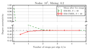
Figure 9: Left: Number of triangles on (const) with $n=$1\text{\times}{10}^{5}$$ and $\mu=1.0$. Right: Degree assortativity on (const) with $n=$1\text{\times}{10}^{7}$$ and $\mu=0.2$. In order to factor in the increased runtime of EM-CM/ES compared to EM-HH, plots of EM-CM/ES are shifted by the runtime of this phase relative to the execution of EM-ES. As EM-CM/ES is a Las-Vegas algorithm, this incurs an additional error along the x-axis.

In section 6, we describe an alternative graph sampling method. Instead of seeding EM-ES with a highly biased graph using EM-HH, we employ the Configuration Model to quickly generate a non-simple random graph. In order to obtain a simple graph, we then carry out several EM-ES runs in a Las-Vegas fashion.

Since EM-ES scans through the edge list in each iteration, runs with very few swaps are inefficient. For this reason, we start the subsequent Markov Chain early: First identify all multi-edges and self-loops and generate swaps with random partners. In a second step, we then introduce additional random swaps until the run contains at least $m/10$ operations.

For an experimental comparison between EM-ES and EM-CM/ES, we consider the runtime until both yield a sufficiently uniform random sample. Of course, the uniformity is hard to quantify; similarly to related studies (cf. section 1.1), we estimate the mixing times of both approaches as follows. Starting from a common seed graph $G^{(0)}$, we generate an ensemble $\{G_{1}^{(k)},\ldots,G_{S}^{(k)}\}$ of $S\gg 1$ instances by applying independent random sequences of $k\gg m$ swaps each. During this process, we regularly export snapshots $G_{i}^{(jm)}$ of the intermediate instances $j\in[k/m]$ of graph $G_{i}$. For EM-CM/ES, we start from the same seed graph, apply the algorithm and then carry out $k$ swaps as described above.

For each snapshot, we compute a number of metrics, such as the average local clustering coefficient (ACC), the number of triangles, and degree assortativity. We then investigate how the distribution of these measures evolves within the ensemble as we carry out an increasing number of swaps. We omit results for ACC since they are less sensitive compared to the other measures (cf. section 10.7).

As illustrated in Fig. 9 and Appendix C, all proxy measures converge within $5m$ swaps with a very small variance. No statistically significant change can be observed compared to a Markov chain with $30m$ operations (which was only computed for a subset of each ensemble). EM-HH generates biased instances with special properties, such as a high number of triangles and correlated node degrees, while the features of EM-CM/ES’s output nearly match the converged ensemble. This suggests that the number of swaps to obtain a sufficiently uniform sample can be reduced for EM-CM/ES.

Due to computational costs, the study was carried out on multiple machines executing several tasks in parallel. Hence, absolute running times are not meaningful, and we rather measure the computational costs in units of time required to carry out $1m$ swaps by the same process. This accounts for the offset of EM-CM/ES’s first data point.

The number of rounds required to obtain a simple graph depends on the degree distribution. For (const) with $n=$1\text{\times}{10}^{5}$$ and $\mu=1$, a fraction of $5.1\text{\,}\mathrm{\char 37\relax}$ of the edges produced by the Configuration Model are illegal. EM-ES requires $18\pm 2$ rewiring runs in case a single swap is used per round to rewire an illegal edge. In the default mode of operation, $5.0\pm 0.0$ rounds suffice as the number of rewiring swaps per illegal edge is doubled in each round. For larger graphs with $n=$1\text{\times}{10}^{7}$$, only $0.07\text{\,}\mathrm{\char 37\relax}$ of edges are illegal and need $2.25\pm 0.4$ rewiring runs.

10.7 Convergence of EM-ES

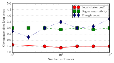
Figure 10: Number of swaps per edge after which ensembles of graphs with (const), $$1\text{\times}{10}^{5}$\leq n\leq$1\text{\times}{10}^{7}$$ and $\mu=0.4$ (left) and $\mu=0.6$ (right) converge. Due to computation costs, the ensemble size is reduced from $S>100$ to $S>10$ for large graphs.

In a similar spirit to the previous section, we indirectly investigate the Markov chain’s mixing time as a function of the number of nodes $n$. To do so, we generate ensembles as before with $$1\text{\times}{10}^{5}$\leq n\leq$1\text{\times}{10}^{7}$$ and compute the same graph metrics. For each group and measure, we then search for the first snapshot $p$ in which the measure’s mean is within an interval of half the standard deviation of the final values and subsequently remains there for at least three phases. We then interpret $p$ as a proxy for the mixing time. As depicted in Fig. 10, no measure shows a systematic increase over the two orders of magnitude considered. It hence seems plausible not to increase the number of swaps performed by EM-LFR compared to the original implementation.

10.8 Performance of EM-LFR

Figure 8 reports the runtime of the original LFR implementation and EM-LFR as a function of the number of nodes $n$ and $\nu=1$. EM-LFR is faster for graphs with $n\geq$2.5\text{\times}{10}^{4}$$ nodes which feature approximately $5\text{\times}{10}^{5}$ edges and are well in the IM domain. Further, the implementation is capable of producing graphs with more than $1\text{\times}{10}^{10}$ edges in $17\text{\,}\mathrm{h}$. Using the same time budget, the original implementation generates graphs more than two orders of magnitude smaller.

10.9 Qualitative Comparison of EM-LFR

When designing EM-LFR, we made sure that it closely follows the LFR benchmark such that we can expect it to produce graphs following the same distribution as the original LFR generator. In order to show experimentally that we achieved this goal, we generated graphs with identical parameters using the original LFR implementation and EM-LFR. For disjoint clusters we also compare it with the implementation that is part of NetworKit [44]. Using NetworKit, we evaluate the results of Infomap [40], Louvain [8] and OSLOM [29], three state-of-the-art clustering algorithms [14, 9, 17], and compare them using the adjusted rand measure [24] and NMI [15].

Figure 11: Adjusted rand measure of Infomap/Louvain and ground truth at $\mu=0.6$ with disjoint clusters, $s_{\min}=10$, $s_{\max}=n/20$.

Figure 12: NMI of OSLOM and ground truth at $\mu=0.4$ with $2$/$4$ overlapping clusters per node.

Figure 13: Average local clustering coefficient at $\mu=0.6$ with disjoint clusters.

Further, we examine the average local clustering coefficient, a measure for the percentage of closed triangles which shows the presence of locally denser areas as expected in communities [25]. We report these measures for graphs ranging from $10^{3}$ to $10^{6}$ nodes. In Fig. 11, 13 and 12 we present a selection of results; all of them can be found in Appendix B. There are only small differences within the range of random noise between the graphs generated by EM-LFR and the other two implementations. Note that due to the computational costs above $10^{5}$ edges, there is only one sample for the original implementation which explains the outliers in Fig. 11. Similar to the results in [14], we also observe that the performance of clustering algorithms drops significantly as the graph’s size grows. This might be due to less clearly defined community structures since the parameters are scaled, and also due to limits of current clustering algorithms. Such behavior clearly demonstrates the necessity of EM-LFR for being able to study this phenomenon on even larger graphs and develop algorithms that are able to handle such instances.

11 Outlook and Conclusion

We propose the first I/O-efficient graph generator for the LFR benchmark and the FDSM, which is the most challenging step involved: EM-HH materializes a graph based on a prescribed degree distribution without I/O for virtually all realistic parameters. Including the generation of a powerlaw degree sequence and the writing of the output to disk, our implementation generates $1.8\text{\times}{10}^{8}$ edges per second for graphs exceeding main memory. EM-ES perturbs existing graphs with $m$ edges based on $k$ edge switches using $\mathcal{O}(k/m\cdot\operatorname{sort}(m))$ I/Os for $k=\Omega(m)$.

We demonstrate that EM-ES is faster than the internal memory implementation [47] even for large instances still fitting in main memory and scales well beyond the limited main memory. Compared to the distributed approach by [7] on a cluster with 128 CPUs, EM-ES exhibits a slow-down of only $8.3$ on one CPU and hence poses a viable and cost-efficient alternative. Our EM-LFR implementation is orders of magnitude faster than the original LFR implementation for large instances and scales well to graphs exceeding main memory while the generated graphs are equivalent. We further gave evidence indicating that commonly accepted parameters to derive the length of the Edge Switching Markov Chain remain valid for graph sizes approaching the external memory domain and that EM-CM/ES can be used to accelerate the process.

Currently, EM-ES does not yet fully exploit the parallelism offered by modern machines. While dependencies between swaps make a parallelization challenging, preliminary experiments indicate that an extension is possible: each run can be split further into smaller batches which can be parallelized in the spirit of [33].

Another possibility for a speedup could be to use the recently proposed Curveball sampling algorithm for graphs with fixed degree sequence [10]. Further studies are necessary to establish whether this really leads to a faster sampling in practice. While the underlying Markov chain seems to require less steps to converge in practice, each step is more expensive. Also, a combination of Curveball with EM-CM/ES seems possible.

Further, this is just the starting point for clustering large graphs that exceed main memory using external memory. Not only are new clustering algorithms needed, but also the evaluation of the results needs to be investigated since existing evaluation measures might not be easily computable in external memory.

Appendix A Summary of Definitions

Symbol	Description
$[k]$	$[k]:=\{1,\ldots,k\}$ for $k\in\mathbb{N}_{+}$ (section 2)
$[u,v]$	Undirected simple edge with implication $u<v$ (section 2)
$B$	Number of items in a block transferred between IM and EM (section 2.1)
$d_{\text{min}}$, $d_{\text{max}}$	Min/max degree of nodes in LFR benchmark (section 3)
$d^{\text{in}}_{v}$	$d^{\text{in}}_{v}=(1{-}\mu)\cdot d_{v}$, intra-community degree of node $v$ (section 3)
$\mathcal{D}$	$\mathcal{D}=(d_{1},\ldots,d_{n})$ with $d_{i}\leq d_{i+1}\forall i$. Degree sequence of a graph (section 4)
$D_{\mathcal{D}}$	$D_{\mathcal{D}}=\big{|}\{d_{i}:1\leq i\leq n\}\big{|}$ where $\mathcal{D}=(d_{1},\ldots,d_{n})$, degree support (section 4)
$n$	Number of vertices in a graph (section 2)
$m$	Number of edges in a graph (section 2)
$\mu$	Mixing parameter in LFR benchmark, i.e. ratio of neighbors that shall be in other communities (section 3)
$M$	Number of items fitting into internal memory (section 2.1)
$\textsc{Pld}\,([a,b),\gamma)$	Powerlaw distribution with exponent $-\gamma$ on the interval $[a,b)$ (section 2)
$s_{\text{min}}$, $s_{\text{max}}$	Min/max size of communities in LFR benchmark (section 3)
$\operatorname{scan}(n)$	$\operatorname{scan}(n)=\Theta(n/B)$ I/Os, scan complexity (section 2.1)
$\operatorname{sort}(n)$	$\operatorname{sort}(n)=\Theta((n/B)\cdot\log_{M/B}(n/B))$ I/Os, sort complexity (section 2.1)

Table 2: Definitions used in this paper.

Appendix B Comparing LFR Implementations

Comparison of the original LFR implementation, the NetworKit implementation and our EM solution for values of $10^{3}\leq n\leq 10^{6}$, $\mu{\in}\{0.2,0.4,0.6\}$, $\gamma{=}2$, $\beta{=}-1$ $d_{\text{min}}{=}10$, $d_{\text{max}}{=}n/20$, $s_{\text{min}}{=}10$, $s_{\text{max}}{=}n/20$. Clustering is performed using Infomap and Louvain and compared to the ground-truth emitted by the generator using AdjustedRandMeasure (AR) and Normalized Mutual Information (NMI); $S\geq 8$. Due to the computational costs, graphs with $n\geq 10^{5}$ have a reduced multiplicity. In case of the original implementation it may be based on a single run which accounts for the few outliers.

 

 

Comparison of the original LFR implementation and our EM solution for values values of $10^{3}\leq n\leq 10^{6}$, $\mu{\in}\{0.2,0.4,0.6\}$, $\nu{\in}\{2,3,4\}$, $O=n$, $\gamma{=}2$, $\beta{=}-1$ $d_{\text{min}}{=}10$, $d_{\text{max}}{=}n/20$, $s_{\text{min}}{=}10\nu$, $s_{\text{max}}{=}\nu\cdot n/20$. Clustering is performed using OSLOM and compared to the ground-truth emitted by the generator using a generalized Normalized Mutual Information (NMI); $S\geq 5$.

Appendix C Comparing EM-ES and EM-CM/ES

Triangle count and degree assortativity of a graph ensemble obtained by applying random swaps/the Configuration Model to a common seed graph. Refer to section 10.6 for experimental details.

References

- [1] Alok Aggarwal and Jeffrey S. Vitter. The input/output complexity of sorting and related problems. Communications of the ACM, 31(9), pages 1116–1127, 1988.
- [2] Omer Angel, Remco van der Hofstad, and Cecilia Holmgren. Limit laws for self-loops and multiple edges in the configuration model. CoRR, abs/1603.07172, 2017. URL: https://arxiv.org/abs/1603.07172.
- [3] Lars Arge. The buffer tree: A new technique for optimal I/O-algorithms (extended abstract). In Algorithms and Data Structures, 4th International Workshop, WADS ’95, Kingston, Ontario, Canada, August 16-18, 1995, Proceedings, pages 334–345, 1995. URL: http://dx.doi.org/10.1007/3-540-60220-8_74, doi:10.1007/3-540-60220-8_74.
- [4] David A. Bader, Henning Meyerhenke, Peter Sanders, Christian Schulz, Andrea Kappes, and Dorothea Wagner. Encyclopedia of Social Network Analysis and Mining, chapter Benchmarking for Graph Clustering and Partitioning, pages 73–82. Springer New York, 2014. URL: http://dx.doi.org/10.1007/978-1-4614-6170-8_23, doi:10.1007/978-1-4614-6170-8_23.
- [5] Andreas Beckmann, Roman Dementiev, and Johannes Singler. Building a parallel pipelined external memory algorithm library. In 23rd IEEE International Symposium on Parallel and Distributed Processing, IPDPS 2009, Rome, Italy, May 23-29, 2009, pages 1–10, 2009. URL: http://dx.doi.org/10.1109/IPDPS.2009.5161001, doi:10.1109/IPDPS.2009.5161001.
- [6] Jon Louis Bentley and James B. Saxe. Generating sorted lists of random numbers. ACM Trans. Math. Softw., 6(3):359–364, 1980. URL: http://doi.acm.org/10.1145/355900.355907, doi:10.1145/355900.355907.
- [7] Hasanuzzaman Bhuiyan, Jiangzhuo Chen, Maleq Khan, and Madhav V. Marathe. Fast parallel algorithms for edge-switching to achieve a target visit rate in heterogeneous graphs. In 43rd International Conference on Parallel Processing, ICPP 2014, Minneapolis, MN, USA, September 9-12, 2014, pages 60–69, 2014. URL: http://dx.doi.org/10.1109/ICPP.2014.15, doi:10.1109/ICPP.2014.15.
- [8] Vincent Blondel, Jean-Loup Guillaume, Renaud Lambiotte, and Etienne Lefebvre. Fast unfolding of communities in large networks. Journal of Statistical Mechanics: Theory and Experiment, 2008(10), 2008. URL: http://dx.doi.org/10.1088/1742-5468/2008/10/P10008.
- [9] Nazar Buzun, Anton Korshunov, Valeriy Avanesov, Ilya Filonenko, Ilya Kozlov, Denis Turdakov, and Hangkyu Kim. Egolp: Fast and distributed community detection in billion-node social networks. In 2014 IEEE International Conference on Data Mining Workshop, pages 533–540, Dec 2014. doi:10.1109/ICDMW.2014.158.
- [10] Corrie Jacobien Carstens, Annabell Berger, and Giovanni Strona. Curveball: a new generation of sampling algorithms for graphs with fixed degree sequence. ArXiv e-prints, September 2016. arXiv:1609.05137.
- [11] Kyrylo Chykhradze, Anton Korshunov, Nazar Buzun, Roman Pastukhov, Nikolay Kuzyurin, Denis Turdakov, and Hangkyu Kim. Distributed generation of billion-node social graphs with overlapping community structure. In Complex Networks V: Proceedings of the 5th Workshop on Complex Networks CompleNet, pages 199–208. Springer International, 2014. URL: http://dx.doi.org/10.1007/978-3-319-05401-8_19, doi:10.1007/978-3-319-05401-8_19.
- [12] Roman Dementiev, Lutz Kettner, and Peter Sanders. STXXL: standard template library for XXL data sets. Softw., Pract. Exper., 38(6):589–637, 2008. URL: http://dx.doi.org/10.1002/spe.844, doi:10.1002/spe.844.
- [13] Roger B. Eggleton and Derek Allan Holton. Simple and multigraphic realizations of degree sequences. In Proceedings of the Eighth Australian Conference on Combinatorial Mathematics, Lecture Notes in Mathematics, pages 155–172. Springer, 1980. URL: http://dx.doi.org/10.1007/BFb0091817.
- [14] Scott Emmons, Stephen G. Kobourov, Mike Gallant, and Katy Börner. Analysis of Network Clustering Algorithms and Cluster Quality Metrics at Scale. PLoS ONE, 11(7):1–18, July 2016. URL: http://dx.doi.org/10.1371/journal.pone.0159161.
- [15] Alcides Viamontes Esquivel and Martin Rosvall. Comparing network covers using mutual information, 2012. arXiv:1202.0425. URL: http://arxiv.org/abs/1202.0425.
- [16] Santo Fortunato. Community detection in graphs. Physics Reports, 486(3-5):75 – 174, 2010. URL: http://www.sciencedirect.com/science/article/pii/S0370157309002841, doi:10.1016/j.physrep.2009.11.002.
- [17] Santo Fortunato and Darko Hric. Community detection in networks: A user guide. Physics Reports, 659:1–44, 2016. URL: https://dx.doi.org/10.1016/j.physrep.2016.09.002.
- [18] Christos Gkantsidis, Milena Mihail, and Ellen W. Zegura. The Markov Chain Simulation Method for Generating Connected Power Law Random Graphs. In Proceedings of the 5th Workshop on Algorithm Engineering and Experiments (ALENEX’03), pages 16–25. SIAM, 2003.
- [19] Catherine S. Greenhill and Matteo Sfragara. The switch markov chain for sampling irregular graphs and digraphs. CoRR, abs/1701.07101, 2017. URL: http://arxiv.org/abs/1701.07101.
- [20] Seifollah L. Hakimi. On realizability of a set of integers as degrees of the vertices of a linear graph. i. Journal of the Society for Industrial and Applied Mathematics, 10(3):496–506, 1962. doi:10.1137/0110037.
- [21] Michael Hamann, Ulrich Meyer, Manuel Penschuck, and Dorothea Wagner. I/O-efficient Generation of Massive Graphs Following the LFR Benchmark. In Proceedings of the 19th Meeting on Algorithm Engineering and Experiments (ALENEX’17), pages 58–72. SIAM, 2017. URL: http://dx.doi.org/10.1137/1.9781611974768.5.
- [22] Steve Harenberg, Gonzalo Bello, L. Gjeltema, Stephen Ranshous, Jitendra Harlalka, Ramona Seay, Kanchana Padmanabhan, and Nagiza Samatova. Community detection in large-scale networks: a survey and empirical evaluation. Wiley Interdisciplinary Reviews: Computational Statistics, 6(6):426–439, 2014. URL: http://dx.doi.org/10.1002/wics.1319, doi:10.1002/wics.1319.
- [23] Václav Havel. Poznámka o existenci konečných grafů. Časopis pro pěstování matematiky, 080(4):477–480, 1955. URL: http://eudml.org/doc/19050.
- [24] Lawrence Hubert and Phipps Arabie. Comparing partitions. Journal of Classification, 2(1):193–218, December 1985. URL: http://dx.doi.org/10.1007/BF01908075.
- [25] Marcus Kaiser. Mean clustering coefficients: the role of isolated nodes and leafs on clustering measures for small-world networks. New Journal of Physics, 10(8), 2008. URL: http://dx.doi.org/10.1088/1367-2630/10/8/083042.
- [26] Panqanamala Ramana Kumar, Martin J Wainwright, and Riccardo Zecchina. Mathematical Foundations of Complex Networked Information Systems: Politecnico Di Torino, Verrès, Italy 2009, volume 2141. Springer, 2015.
- [27] Andrea Lancichinetti and Santo Fortunato. Benchmarks for testing community detection algorithms on directed and weighted graphs with overlapping communities. Phys. Rev. E, 80:016118, Jul 2009. Source code available at https://sites.google.com/site/santofortunato/inthepress2. URL: http://link.aps.org/doi/10.1103/PhysRevE.80.016118, doi:10.1103/PhysRevE.80.016118.
- [28] Andrea Lancichinetti, Santo Fortunato, and Filippo Radicchi. Benchmark graphs for testing community detection algorithms. Phys. Rev. E, 78:046110, Oct 2008. URL: http://link.aps.org/doi/10.1103/PhysRevE.78.046110, doi:10.1103/PhysRevE.78.046110.
- [29] Andrea Lancichinetti, Filippo Radicchi, José J. Ramasco, and Santo Fortunato. Finding Statistically Significant Communities in Networks. PLoS ONE, 6(4):1–18, April 2011. URL: http://dx.doi.org/10.1371/journal.pone.0018961.
- [30] Jure Leskovec, Jon M. Kleinberg, and Christos Faloutsos. Graphs Over Time: Densification Laws, Shrinking Diameters and Possible Explanations. In Proceedings of the 11th ACM SIGKDD International Conference on Knowledge Discovery and Data Mining, pages 177–187. ACM Press, 2005. URL: http://portal.acm.org/citation.cfm?id=1081893.
- [31] Anil Maheshwari and Norbert Zeh. A survey of techniques for designing I/O-efficient algorithms. In Algorithms for Memory Hierarchies, pages 36–61, 2003. URL: http://dx.doi.org/10.1007/3-540-36574-5_3, doi:10.1007/3-540-36574-5_3.
- [32] Ulrich Meyer and Manuel Penschuck. Generating massive scale-free networks under resource constraints. In Proceedings of the Eighteenth Workshop on Algorithm Engineering and Experiments (ALENEX 2016), pages 39–52, 2016. URL: http://epubs.siam.org/doi/abs/10.1137/1.9781611974317.4, doi:10.1137/1.9781611974317.4.
- [33] Ulrich Meyer and Peter Sanders. Delta-stepping: A parallel single source shortest path algorithm. In Algorithms - ESA ’98, 6th Annual European Symposium, Venice, Italy, August 24-26, 1998, Proceedings, pages 393–404, 1998. URL: http://dx.doi.org/10.1007/3-540-68530-8_33, doi:10.1007/3-540-68530-8_33.
- [34] Ulrich Meyer, Peter Sanders, and Jop F. Sibeyn, editors. Algorithms for Memory Hierarchies, Advanced Lectures [Dagstuhl Research Seminar, March 10-14, 2002], volume 2625 of Lecture Notes in Computer Science. Springer, 2003.
- [35] Ron Milo, Nadav Kashtan, Shalev Itzkovitz, Mark E. J. Newman, and Uri. Alon. On the uniform generation of random graphs with prescribed degree sequences. eprint arXiv:cond-mat/0312028, December 2003. arXiv:cond-mat/0312028.
- [36] Rajeev Motwani and Prabhakar Raghavan. Randomized algorithms. Chapman & Hall/CRC, 2010.
- [37] Mark Newman. Networks: An Introduction. Oxford University Press, Inc., New York, NY, USA, 2010.
- [38] Rasmus Pagh. Basic external memory data structures. In Algorithms for Memory Hierarchies, pages 14–35. Springer, 2003.
- [39] Jaideep Ray, Ali Pinar, and C. Seshadhri. Are We There Yet? When to Stop a Markov Chain while Generating Random Graphs. In Algorithms and Models for the Web-Graph, Proceedings of the 9th International Workshop, WAW 2012, Lecture Notes in Computer Science, pages 153–164. Springer, 2012. URL: https://doi.org/10.1007/978-3-642-30541-2_12.
- [40] Martin Rosvall, Daniel Axelsson, and Carl T. Bergstrom. The map equation. The European Physical Journal Special Topics, 178(1):13–23, 2009. URL: http://dx.doi.org/10.1140/epjst/e2010-01179-1.
- [41] Peter Sanders. Random permutations on distributed, external and hierarchical memory. Inf. Process. Lett., 67(6):305–309, 1998. URL: http://dx.doi.org/10.1016/S0020-0190(98)00127-6, doi:10.1016/S0020-0190(98)00127-6.
- [42] Peter Sanders. Fast priority queues for cached memory. Journal of Experimental Algorithmics (JEA), 5, 2000.
- [43] Wolfgang E. Schlauch, Emőke Ágnes Horvát, and Katharina A. Zweig. Different flavors of randomness: comparing random graph models with fixed degree sequences. Social Network Analysis and Mining, 5(1):1–14, 2015. URL: http://dx.doi.org/10.1007/s13278-015-0267-z, doi:10.1007/s13278-015-0267-z.
- [44] Christian Staudt, Aleksejs Sazonovs, and Henning Meyerhenke. Networkit: A tool suite for large-scale complex network analysis. Network Science, 4(4):508–530, 2016. doi:10.1017/nws.2016.20.
- [45] The Lemur Project. ClueWeb12 Web Graph, Nov 2013. http://www.lemurproject.org/clueweb12/webgraph.php.
- [46] Johan Ugander, Brian Karrer, Lars Backstrom, and Cameron Marlow. The anatomy of the facebook social graph. CoRR, abs/1111.4503, 2011. URL: http://arxiv.org/abs/1111.4503.
- [47] Fabien Viger and Matthieu Latapy. Fast generation of random connected graphs with prescribed degrees. CoRR, abs/cs/0502085, 2005. Source code available at https://www-complexnetworks.lip6.fr/~latapy/FV/generation.html. URL: http://arxiv.org/abs/cs/0502085.
- [48] Jeffrey Scott Vitter. An efficient algorithm for sequential random sampling. ACM Trans. Math. Softw., 13(1):58–67, 1987. URL: http://doi.acm.org/10.1145/23002.23003, doi:10.1145/23002.23003.
- [49] Jianping Zeng and Hongfeng Yu. A study of graph partitioning schemes for parallel graph community detection. Parallel Computing, 2016. URL: http://dx.doi.org/10.1016/j.parco.2016.05.008.
- [50] James Y. Zhao. Expand and contract: Sampling graphs with given degrees and other combinatorial families. CoRR, abs/1308.6627, 2013. URL: http://arxiv.org/abs/1308.6627.