JLQCD collaboration

Renormalization of domain-wall bilinear operators with short-distance current correlators

M. Tomii tomii@post.kek.jp Department of Particle and Nuclear Science, SOKENDAI (The Graduate University for Advanced Studies), Tsukuba 305-0801, Japan Theory Center, Institute of Particle and Nuclear Studies, High Energy Accelerator Research Organization (KEK), Tsukuba 305-0801, Japan    G. Cossu Theory Center, Institute of Particle and Nuclear Studies, High Energy Accelerator Research Organization (KEK), Tsukuba 305-0801, Japan    B. Fahy Theory Center, Institute of Particle and Nuclear Studies, High Energy Accelerator Research Organization (KEK), Tsukuba 305-0801, Japan    H. Fukaya Department of Physics, Osaka University, Toyonaka 560-0043, Japan    S. Hashimoto Department of Particle and Nuclear Science, SOKENDAI (The Graduate University for Advanced Studies), Tsukuba 305-0801, Japan Theory Center, Institute of Particle and Nuclear Studies, High Energy Accelerator Research Organization (KEK), Tsukuba 305-0801, Japan    T. Kaneko Department of Particle and Nuclear Science, SOKENDAI (The Graduate University for Advanced Studies), Tsukuba 305-0801, Japan Theory Center, Institute of Particle and Nuclear Studies, High Energy Accelerator Research Organization (KEK), Tsukuba 305-0801, Japan    J. Noaki Theory Center, Institute of Particle and Nuclear Studies, High Energy Accelerator Research Organization (KEK), Tsukuba 305-0801, Japan
Abstract

We determine the renormalization constants for flavor non-singlet fermion bilinear operators of Möbius domain-wall fermions. The renormalization condition is imposed on the correlation functions in the coordinate space, such that the non-perturbative lattice calculation reproduces the perturbatively calculated counterpart at short distances. The perturbative expansion is precise as the coefficients are available up to O(αs4)𝑂superscriptsubscript𝛼𝑠4O(\alpha_{s}^{4}). We employ 2+1212+1-flavor lattice ensembles at three lattice spacings in the range 0.044–0.080 fm.

preprint: KEK-CP-344, OU-HET-894

I Introduction

Renormalization of lattice operators is a necessary step for the lattice QCD calculations of scheme-dependent quantities such as the matrix elements of the weak effective Hamiltonian, which contains composite operators of quark fields such as bilinear and four-fermion operators. In phenomenological studies, comparison of lattice results with experimental values or theoretical results from other approaches has to be performed with a matched renormalization scheme and scale. The conventional choice for this is the MS¯¯MS\rm\overline{MS} scheme. Among bilinear operators, vector (and axial-vector) currents are simplest because they are not renormalized because of current conservation. On the lattice, however, the commonly used local vector current is not conserved at finite lattice spacing and a finite renormalization to match the continuum counterpart is necessary. The axial-current is renormalized differently unless the lattice fermion formulation respects chiral symmetry. Scale dependent operators such as scalar and pseudoscalar currents require renormalization in any case.

Matching to the continuum renormalization scheme necessarily involves perturbation theory, since the MS¯¯MS\rm\overline{MS} scheme adopted in the continuum theory is inherently perturbative. It means that the renormalization condition must be applied at momentum scale of 2 GeV or higher, where QCD becomes perturbative. In this regime, the discretization effect of lattice theory becomes significant as typical value of lattice cutoff for currently available ensembles is 2–3 GeV. This causes the so-called window problem, which implies that one has to identify a window of momentum scale where the systematic uncertainties of perturbative and lattice calculations are controlled. One of the widely used method is the non-perturbative renormalization through the RI/MOM scheme as an intermediate renormalization condition Martinelli:1994ty . In this method, one calculates the vertex function involving the composite operator of interest with a certain momentum configuration of external quarks in a fixed gauge. The external momenta are carefully chosen to satisfy the window condition as mentioned above. In many cases, one can find the region where the discretization effect is under control by inspecting the momentum dependence of the obtained vertex function. The convergence of the perturbative expansion, on the other hand, is not well tested, as the perturbative expansion is available only at the one- or two-loop level in many cases. In fact, this is a dominant source of systematic uncertainty in this method.

In this work, we adopt another renormalization condition, which is called the coordinate space method or the X-space method. The method was first proposed in Martinelli:1997zc and has so far been applied in Gimenez:2004me ; Cichy:2012is . In this method, the renormalization condition is imposed on the correlation function at a certain distance in the coordinate space. The correlation functions are those of composite operators of interest. A typical example is a correlation function of vector currents u¯γμd(x)¯𝑢subscript𝛾𝜇𝑑𝑥\bar{u}\gamma_{\mu}d(x) and d¯γνu(y)¯𝑑subscript𝛾𝜈𝑢𝑦\bar{d}\gamma_{\nu}u(y) placed at certain points x𝑥x and y𝑦y in the coordinate space. Here, u𝑢u and d𝑑d denote the up and down quark fields, respectively. The correlation function thus constructed u¯γμd(x)d¯γνu(y)delimited-⟨⟩¯𝑢subscript𝛾𝜇𝑑𝑥¯𝑑subscript𝛾𝜈𝑢𝑦\langle\bar{u}\gamma_{\mu}d(x)\bar{d}\gamma_{\nu}u(y)\rangle is gauge invariant, and more importantly it is a common object in the continuum QCD for which the state-of-the-art techniques of perturbative QCD have been applied. For the (axial-)vector and (pseudo)scalar correlators, the perturbative series has been calculated to the order of αs4superscriptsubscript𝛼𝑠4\alpha_{s}^{4} Chetyrkin:2010dx , with which the uncertainty due to a truncation of the perturbative series is highly suppressed and the remaining uncertainty is reliably estimated using the convergence behavior of the series. Another important advantage of the X-space method is that the X-space correlator does not involve extra divergences other than those of the operators involved, because of the finite distance between x𝑥x and y𝑦y. The corresponding correlator in the momentum space has an extra divergence from a loop contracting the two points, and one has to consider a derivative in the momentum space to extract a well-defined quantity.

The window problem does exist for the X-space method. The distance between x𝑥x and y𝑦y must be sufficiently small for perturbation theory to be convergent, and at the same time it has to be large compared to the lattice spacing a𝑎a. The main point of this work is therefore to identify such a region. On the perturbative side, we investigate the convergence property of the perturbative series known to αs4superscriptsubscript𝛼𝑠4\alpha_{s}^{4}. The convergence can be improved by optimizing the scale μ𝜇\mu of coupling constant αs(μ)subscript𝛼𝑠𝜇\alpha_{s}(\mu), depending on the distance |xy|𝑥𝑦|x-y|. We first attempt the use of the Brodsky-Lepage-Mackenzie (BLM) scale setting procedure Brodsky:1982gc , which in fact leads to a much improved convergence compared to a naïve choice of μ=1/|xy|𝜇1𝑥𝑦\mu=1/|x-y|. In order to estimate the remaining uncertainty due to the truncation of higher order terms, we vary the scale in some range and inspect the stability of the result. A detailed account of this study is given in Section III for both vector and scalar correlators.

As we include the longer-distance correlators in the analysis, non-perturbative power corrections could also appear as well as the problem of increasingly less convergent perturbative series. Such effect is described by the Operator Product Expansion (OPE) Shifman:1978bx . The leading contribution comes from the dimension-four operators: the quark condensate and gluon condensate. The quark condensate appears with a quark mass, and induces a linear dependence on the quark mass. We confirm that the lattice data are consistent with the prediction of OPE. We can then eliminate this type of power correction by combining vector and axial-vector correlators with appropriate factors. Similar method is also applied for scalar and pseudoscalar correlators. The effect of gluon condensate is more difficult to identify. We fit the lattice data to the corresponding functional form in |xy|𝑥𝑦|x-y|.

At short distances on the lattice, the discretization error is a major concern, which we investigate in detail in Section IV. The discretization effect is indeed very substantial at the distance of |xy|/aless-than-or-similar-to𝑥𝑦𝑎absent|x-y|/a\lesssim 10. Fortunately, most of such effects can be eliminated by subtracting the correlators calculated at the tree-level (or mean-field improved). Further reduction can be achieved by selecting the direction of the points on the lattice. These improvements have already been applied in the previous studies Gimenez:2004me ; Cichy:2012is , and we refine them to minimize the remaining errors. Even after such reductions of errors, the discretization effects are still significant at the level of 3–5% for the correlators. We attempt to eliminate them by using the lattice data available for us at three different lattice spacings in the range 0.044–0.080 fm. We fit the lattice data at short distances assuming that the leading discretization effect is O(a2)𝑂superscript𝑎2O(a^{2}), and subtract it. The remaining error is then at the level of one per cent.

In this work, we determine the renormalization constants for the vector (and axial-vector) current and scalar (and pseudoscalar) density operator composed of the Möbius domain-wall fermions Brower:2004xi ; Brower:2012vk . Möbius domain-wall fermion is an improved implementation of the domain-wall fermion Kaplan:1992bt ; Shamir:1993zy . The four-dimensional effective Dirac operator of the domain-wall fermion precisely satisfies the Ginsparg-Wilson relation and thus respects the modified chiral symmetry on the lattice. It implies that the vector and axial-vector renormalization factors are equal to each other to a good precision. With the Möbius implementation, the residual mass, which quantifies the size of the Ginsparg-Wilson violation, is at the order of 1 MeV or less on our lattice ensembles. For the determination of the renormalization constants, this amount of violation can be safely neglected. In fact, we confirm that the corresponding current correlators agree very precisely at short distances where the effect of the quark condensate is negligible.

This paper is organized as follows. In Section II, we describe the basic strategy to determine the renormalization constants. In Section III, we discuss the detail of massless correlators in perturbation theory and the improvement of their convergence. After that, we give the contribution of OPE to the correlators. In Section IV, we show the analyses of lattice calculation including our lattice setup and some managements of lattice artifacts. In Section V, we explain the detail of determination of the renormalization factors and show the final results.

II Renormalization condition in the X-space method

In the X-space method, the renormalization constants are determined by analyzing two-point correlation functions at finite separation xy𝑥𝑦x-y. In this work, we consider the following four channels of flavor non-singlet correlators in the coordinate space,

ΠS(x)=S(x)S(0),ΠP(x)=P(x)P(0),ΠV(x)=μVμ(x)Vμ(0),ΠA(x)=μAμ(x)Aμ(0),subscriptΠ𝑆𝑥delimited-⟨⟩𝑆𝑥𝑆superscript0subscriptΠ𝑃𝑥delimited-⟨⟩𝑃𝑥𝑃superscript0subscriptΠ𝑉𝑥subscript𝜇delimited-⟨⟩subscript𝑉𝜇𝑥subscript𝑉𝜇superscript0subscriptΠ𝐴𝑥subscript𝜇delimited-⟨⟩subscript𝐴𝜇𝑥subscript𝐴𝜇superscript0\begin{array}[]{ll}\Pi_{S}(x)=\langle S(x)S(0)^{\dagger}\rangle,&\hskip 28.45274pt\Pi_{P}(x)=\langle P(x)P(0)^{\dagger}\rangle,\\ \Pi_{V}(x)=\sum_{\mu}\langle V_{\mu}(x)V_{\mu}(0)^{\dagger}\rangle,&\hskip 28.45274pt\Pi_{A}(x)=\sum_{\mu}\langle A_{\mu}(x)A_{\mu}(0)^{\dagger}\rangle,\end{array} (1)

where each operator is composed of (mass degenerate) up and down quark fields u(x)𝑢𝑥u(x) and d(x)𝑑𝑥d(x),

S(x)=u¯(x)d(x),P(x)=u¯(x)iγ5d(x),Vμ(x)=u¯(x)γμd(x),Aμ(x)=u¯(x)γμγ5d(x).𝑆𝑥¯𝑢𝑥𝑑𝑥𝑃𝑥¯𝑢𝑥isubscript𝛾5𝑑𝑥subscript𝑉𝜇𝑥¯𝑢𝑥subscript𝛾𝜇𝑑𝑥subscript𝐴𝜇𝑥¯𝑢𝑥subscript𝛾𝜇subscript𝛾5𝑑𝑥\begin{array}[]{ll}S(x)=\bar{u}(x)d(x),&\hskip 28.45274ptP(x)=\bar{u}(x){\rm{i}}\gamma_{5}d(x),\\ V_{\mu}(x)=\bar{u}(x)\gamma_{\mu}d(x),&\hskip 28.45274ptA_{\mu}(x)=\bar{u}(x)\gamma_{\mu}\gamma_{5}d(x).\end{array} (2)

Here, the coordinate y𝑦y of the source point is fixed at origin and correlators are parametrized by a four-dimensional coordinate x𝑥x with an assumption of translational invariance.

We renormalize the quark bilinear operators on the lattice to those in the MS¯¯MS\rm\overline{MS} scheme at a renormalization scale, which is often set to 2 or 3 GeV. Neglecting the contributions of irrelevant operators, the renormalization is multiplicative, i.e.

OΓMS¯(2GeV;x)=ZΓMS¯/lat(2GeV,a)OΓlat(a;x),superscriptsubscript𝑂Γ¯MS2GeV𝑥superscriptsubscript𝑍Γ¯MSlat2GeV𝑎superscriptsubscript𝑂Γlat𝑎𝑥O_{\Gamma}^{\rm\overline{MS}}(2{\rm\ GeV};x)=Z_{\Gamma}^{\rm\overline{MS}/lat}(2{\rm\ GeV},a)O_{\Gamma}^{\rm lat}(a;x), (3)

where Γ{S,P,V,A}Γ𝑆𝑃𝑉𝐴\Gamma\in\{S,P,V,A\}, OΓ{S,P,Vμ,Aμ}subscript𝑂Γ𝑆𝑃subscript𝑉𝜇subscript𝐴𝜇O_{\Gamma}\in\{S,P,V_{\mu},A_{\mu}\}, and ZΓMS¯/lat(2GeV,a)superscriptsubscript𝑍Γ¯MSlat2GeV𝑎Z_{\Gamma}^{\rm\overline{MS}/lat}(2{\rm\ GeV},a) is the renormalization constant. The renormalization condition in the X-space method is imposed by requiring

(Z~ΓMS¯/lat(2GeV,a;x))2ΠΓlat(a;x)=ΠΓMS¯(2GeV;x),superscriptsuperscriptsubscript~𝑍Γ¯MSlat2GeV𝑎𝑥2superscriptsubscriptΠΓlat𝑎𝑥superscriptsubscriptΠΓ¯MS2GeV𝑥\Big{(}\widetilde{Z}_{\Gamma}^{\rm\overline{MS}/lat}(2{\rm\ GeV},a;x)\Big{)}^{2}\Pi_{\Gamma}^{\rm lat}(a;x)=\Pi_{\Gamma}^{\rm\overline{MS}}(2{\rm\ GeV};x), (4)

or

Z~ΓMS¯/lat(2GeV,a;x)=ΠΓMS¯(2GeV;x)ΠΓlat(a;x),superscriptsubscript~𝑍Γ¯MSlat2GeV𝑎𝑥superscriptsubscriptΠΓ¯MS2GeV𝑥superscriptsubscriptΠΓlat𝑎𝑥\widetilde{Z}_{\Gamma}^{\rm\overline{MS}/lat}(2{\rm\ GeV},a;x)=\sqrt{\Pi_{\Gamma}^{\rm\overline{MS}}(2{\rm\ GeV};x)\over\Pi_{\Gamma}^{\rm lat}(a;x)}, (5)

at a finite distance x𝑥x. Note that Z~ΓMS¯/lat(2GeV,a;x)superscriptsubscript~𝑍Γ¯MSlat2GeV𝑎𝑥\widetilde{Z}_{\Gamma}^{\rm\overline{MS}/lat}(2{\rm\ GeV},a;x) still contains some dependence on x𝑥x. It originates from errors arising in the continuum ΠΓMS¯(2GeV;x)superscriptsubscriptΠΓ¯MS2GeV𝑥\Pi_{\Gamma}^{\rm\overline{MS}}(2{\rm\ GeV};x) and lattice ΠΓlat(a;x)superscriptsubscriptΠΓlat𝑎𝑥\Pi_{\Gamma}^{\rm lat}(a;x) correlators. The continuum one suffers from truncation of the perturbative expansion as we discuss in the following sections. On the other hand, the lattice correlator contains discretization effects. In addition, the x𝑥x-dependence of Z~ΓMS¯/lat(2GeV,a;x)superscriptsubscript~𝑍Γ¯MSlat2GeV𝑎𝑥\widetilde{Z}_{\Gamma}^{\rm\overline{MS}/lat}(2{\rm\ GeV},a;x) is also caused by non-perturbative effects at large |x|𝑥|x| in full QCD, which are not encoded in the continuum perturbative correlator. In order to extract the renormalization constant, which must be independent of x𝑥x, the distance |x|𝑥|x| of correlators should be chosen in a window a|x|1/ΛQCDmuch-less-than𝑎𝑥much-less-than1subscriptΛQCDa\ll|x|\ll 1/\Lambda_{\rm QCD} to suppress these possible errors. In Section V, the systematic effects arising in Z~ΓMS¯(2GeV,a;x)superscriptsubscript~𝑍Γ¯MS2GeV𝑎𝑥\widetilde{Z}_{\Gamma}^{\rm\overline{MS}}({2\rm\ GeV},a;x) are discussed in more detail and the renormalization factor ZΓMS¯(2GeV,a)superscriptsubscript𝑍Γ¯MS2GeV𝑎Z_{\Gamma}^{\rm\overline{MS}}({2\rm\ GeV},a) is determined.

III Continuum theory

III.1 Massless perturbation theory

In this subsection, we discuss the convergence of the perturbative expansion of the massless correlators. Since the scalar and pseudoscalar correlators, as well as the vector and axial-vector correlators, degenerate in the massless perturbation theory, i.e. ΠS=ΠPsubscriptΠ𝑆subscriptΠ𝑃\Pi_{S}=\Pi_{P} and ΠV=ΠAsubscriptΠ𝑉subscriptΠ𝐴\Pi_{V}=\Pi_{A}, we consider only the two channels ΠSsubscriptΠ𝑆\Pi_{S} and ΠVsubscriptΠ𝑉\Pi_{V}.

The perturbative expansion of the vector correlator is written as

ΠVMS¯(x)=6π4x6(1+i=1CiVas(μx)i),superscriptsubscriptΠ𝑉¯MS𝑥6superscript𝜋4superscript𝑥61superscriptsubscript𝑖1superscriptsubscript𝐶𝑖𝑉subscript𝑎𝑠superscriptsubscript𝜇𝑥𝑖\Pi_{V}^{\rm\overline{MS}}(x)={6\over\pi^{4}x^{6}}\left(1+\sum_{i=1}^{\infty}C_{i}^{V}a_{s}(\mu_{x})^{i}\right), (6)

with perturbative coefficients CiVsuperscriptsubscript𝐶𝑖𝑉C_{i}^{V}. Here, as(μx)=αs(μx)/πsubscript𝑎𝑠subscript𝜇𝑥subscript𝛼𝑠subscript𝜇𝑥𝜋a_{s}(\mu_{x})=\alpha_{s}(\mu_{x})/\pi is the strong coupling constant and its scale μxsubscript𝜇𝑥\mu_{x} is set as

μx=1|x|.subscript𝜇𝑥1𝑥\mu_{x}={1\over|x|}. (7)

One can reorganize the perturbative series using the renormalization group to another scale μxsuperscriptsubscript𝜇𝑥\mu_{x}^{*}, i.e.

ΠVMS¯(x)=6π4x6(1+i=1CiV(μx)as(μx)i),superscriptsubscriptΠ𝑉¯MS𝑥6superscript𝜋4superscript𝑥61superscriptsubscript𝑖1superscriptsubscript𝐶𝑖𝑉superscriptsubscript𝜇𝑥subscript𝑎𝑠superscriptsuperscriptsubscript𝜇𝑥𝑖\Pi_{V}^{\rm\overline{MS}}(x)={6\over\pi^{4}x^{6}}\left(1+\sum_{i=1}^{\infty}C_{i}^{V}(\mu_{x}^{*})a_{s}(\mu_{x}^{*})^{i}\right), (8)

which is exact when the perturbative series includes all orders, provided that the coefficients CiV(μx)subscriptsuperscript𝐶𝑉𝑖subscriptsuperscript𝜇𝑥C^{V}_{i}(\mu^{*}_{x}) are converted appropriately. The conversion formula of the coupling constants is available to four-loop level vanRitbergen:1997va .

Chetyrkin and Maier Chetyrkin:2010dx wrote the perturbative coefficients up to O(as4)𝑂superscriptsubscript𝑎𝑠4O(a_{s}^{4}) at the renormalization scale μxsubscript𝜇𝑥\mu_{x} in the MS~~MS\rm\widetilde{MS} scheme, which is the same as the MS¯¯MS\rm\overline{MS} scheme at a scale μ~x=2eγEμx1.123/|x|subscript~𝜇𝑥2superscriptesubscript𝛾𝐸subscript𝜇𝑥similar-to-or-equals1.123𝑥\tilde{\mu}_{x}=2{\rm{e}}^{-\gamma_{E}}\mu_{x}\simeq 1.123/|x|. Here, γE=0.5772subscript𝛾𝐸0.5772\gamma_{E}=0.5772\ldots is Euler’s constant. In our notation, these coefficients correspond to CiV(μ~x)superscriptsubscript𝐶𝑖𝑉subscript~𝜇𝑥C_{i}^{V}(\tilde{\mu}_{x}). The perturbative coefficients CiV(μx)superscriptsubscript𝐶𝑖𝑉superscriptsubscript𝜇𝑥C_{i}^{V}(\mu_{x}^{*}) at μx=μx,μ~xsuperscriptsubscript𝜇𝑥subscript𝜇𝑥subscript~𝜇𝑥\mu_{x}^{*}=\mu_{x},\tilde{\mu}_{x} obtained by using the results of Chetyrkin:2010dx and vanRitbergen:1997va are summarized in Appendix A.

Since the perturbative expansion truncated at a finite order may depend on μxsuperscriptsubscript𝜇𝑥\mu_{x}^{*}, there is an optimal choice for the scale that leads to a good convergence. One possible recipe to choose the optimal scale μxsuperscriptsubscript𝜇𝑥\mu_{x}^{*} is the Brodsky-Lepage-Mackenzie (BLM) approach Brodsky:1982gc , which is motivated by an idea of absorbing the higher order contributions of gluon vacuum polarization into the coupling constant. The scale is chosen such that the perturbative coefficient at as2superscriptsubscript𝑎𝑠2a_{s}^{2} becomes independent of the number of flavors nfsubscript𝑛𝑓n_{f}. This BLM scale μxBLMsuperscriptsubscript𝜇𝑥BLM\mu_{x}^{\rm BLM} of the vector correlator thus determined is

μxBLM=2exp[12(4ζ332γE)]μx2.7733|x|,superscriptsubscript𝜇𝑥BLM2124subscript𝜁332subscript𝛾𝐸subscript𝜇𝑥similar-to-or-equals2.7733𝑥\mu_{x}^{\rm BLM}=2\exp\left[{1\over 2}(4\zeta_{3}-3-2\gamma_{E})\right]\mu_{x}\simeq{2.7733\over|x|}, (9)

where ζ31.2021similar-to-or-equalssubscript𝜁31.2021\zeta_{3}\simeq 1.2021. The perturbative coefficients CiV(μxBLM)superscriptsubscript𝐶𝑖𝑉superscriptsubscript𝜇𝑥BLMC_{i}^{V}(\mu_{x}^{\rm BLM}) at the BLM scale are summarized in Appendix A.
Refer to caption
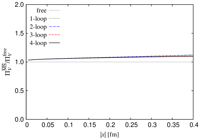
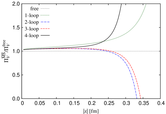
Figure 1: Perturbative expansion of the vector correlator renormalized in the MS¯¯MS\rm\overline{MS} scheme with nf=3subscript𝑛𝑓3n_{f}=3. The results at μx=μxsuperscriptsubscript𝜇𝑥subscript𝜇𝑥\mu_{x}^{*}=\mu_{x} truncated at as0superscriptsubscript𝑎𝑠0a_{s}^{0} (fine-dotted), assubscript𝑎𝑠a_{s} (dotted), as2superscriptsubscript𝑎𝑠2a_{s}^{2} (dashed double-dotted), as3superscriptsubscript𝑎𝑠3a_{s}^{3} (dashed dotted), and as4superscriptsubscript𝑎𝑠4a_{s}^{4} (solid) are plotted as functions of |x|𝑥|x|.
Refer to caption
Figure 2: Perturbative expansion of the vector correlator renormalized in the MS¯¯MS\rm\overline{MS} scheme with nf=3subscript𝑛𝑓3n_{f}=3. The results at μx=μxBLMsuperscriptsubscript𝜇𝑥superscriptsubscript𝜇𝑥BLM\mu_{x}^{*}=\mu_{x}^{\rm BLM} truncated at as0superscriptsubscript𝑎𝑠0a_{s}^{0} (fine-dotted), assubscript𝑎𝑠a_{s} (dotted), as2superscriptsubscript𝑎𝑠2a_{s}^{2} (dashed double-dotted), as3superscriptsubscript𝑎𝑠3a_{s}^{3} (dashed dotted), and as4superscriptsubscript𝑎𝑠4a_{s}^{4} (solid) are plotted as functions of |x|𝑥|x|.

Figure 2 shows the vector correlator calculated with μx=μxsuperscriptsubscript𝜇𝑥subscript𝜇𝑥\mu_{x}^{*}=\mu_{x} and nf=3subscript𝑛𝑓3n_{f}=3. It is normalized by the tree-level correlator ΠVfree(x)=6/π4x6superscriptsubscriptΠ𝑉free𝑥6superscript𝜋4superscript𝑥6\Pi_{V}^{\rm free}(x)=6/\pi^{4}x^{6}. A reasonable convergence is observed only below |x|0.15similar-to𝑥0.15|x|\sim 0.15 fm, which is not so large compared to our lattice spacings a=𝑎absenta= 0.044–0.080 fm. It implies that there is no renormalization window satisfying the condition that the perturbative calculation is convergent and the discretization effects are sufficiently small. The convergence of the perturbative series at μx=μ~xsuperscriptsubscript𝜇𝑥subscript~𝜇𝑥\mu_{x}^{*}=\tilde{\mu}_{x} is similar to that at μx=μxsuperscriptsubscript𝜇𝑥subscript𝜇𝑥\mu_{x}^{*}=\mu_{x}. On the other hand, the result at μx=μxBLMsuperscriptsubscript𝜇𝑥superscriptsubscript𝜇𝑥BLM\mu_{x}^{*}=\mu_{x}^{\rm BLM} with nf=3subscript𝑛𝑓3n_{f}=3 shows much better convergence as plotted in Fig. 2, implying that the convergence of the perturbative series is actually improved by tuning the renormalization scale μxsuperscriptsubscript𝜇𝑥\mu_{x}^{*}.

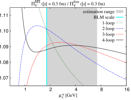
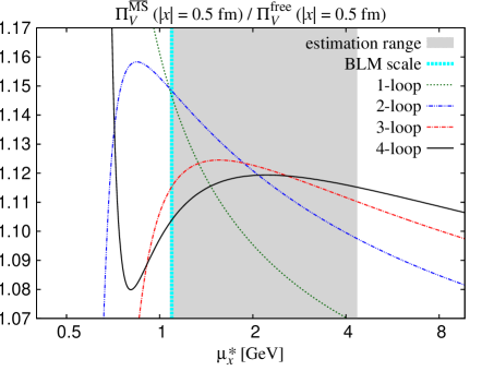
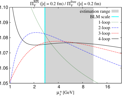
In order to choose the optimal scale and estimate the uncertainty of the higher order corrections, we investigate the μxsuperscriptsubscript𝜇𝑥\mu_{x}^{*}-dependence of the perturbative calculation. The μxsuperscriptsubscript𝜇𝑥\mu_{x}^{*}-dependence of the vector correlator with nf=3subscript𝑛𝑓3n_{f}=3 is shown in Fig. 3 for several distances in the range 0.2–0.5 fm. Since the all-order calculation has to be independent of μxsuperscriptsubscript𝜇𝑥\mu_{x}^{*}, we determine the optimal scale μx,optsuperscriptsubscript𝜇𝑥opt\mu_{x}^{\rm*,opt} as the value which minimizes the μxsuperscriptsubscript𝜇𝑥\mu_{x}^{*}-derivative of the four-loop correlator,

μx,opt=e1.7μx5.5|x|.superscriptsubscript𝜇𝑥optsuperscripte1.7subscript𝜇𝑥similar-to-or-equals5.5𝑥\mu_{x}^{\rm*,opt}={\rm{e}}^{1.7}\mu_{x}\simeq{5.5\over|x|}. (10)

The uncertainty of the higher order corrections to the vector correlator is estimated by varying μxsuperscriptsubscript𝜇𝑥\mu_{x}^{*} in the region [12μx,opt,2μx,opt]12superscriptsubscript𝜇𝑥opt2superscriptsubscript𝜇𝑥opt[{1\over 2}\mu_{x}^{\rm*,opt},2\mu_{x}^{\rm*,opt}], which is shown in Fig. 3 by the gray band.
Refer to caption

Refer to caption

Refer to caption

Refer to caption

Figure 3: Vector correlator renormalized in the MS¯¯MS\rm\overline{MS} scheme at the specific distances 0.2 fm (top/left), 0.3 fm (top/right), 0.4 fm (bottom/left), and 0.5 fm (bottom/right) as functions of μxsubscriptsuperscript𝜇𝑥\mu^{*}_{x}. The results with nf=3subscript𝑛𝑓3n_{f}=3 truncated at assubscript𝑎𝑠a_{s} (dotted), as2superscriptsubscript𝑎𝑠2a_{s}^{2} (dashed double-dotted), as3superscriptsubscript𝑎𝑠3a_{s}^{3} (dashed dotted), and as4superscriptsubscript𝑎𝑠4a_{s}^{4} (solid) are plotted. The gray band represents the region in which we estimate the uncertainty of the higher order corrections. The vertical bold line near the lower end of the gray band stands for the BLM scale (9).

The expansion at the scale μx,optsuperscriptsubscript𝜇𝑥opt\mu_{x}^{\rm*,opt} reads

ΠVMS¯(x)|nf=3=6π4x6(1\displaystyle\Pi_{V}^{\rm\overline{MS}}(x)\bigg{|}_{n_{f}=3}={6\over\pi^{4}x^{6}}\Big{(}1 +as(μx,opt)+3.1431as(μx,opt)2subscript𝑎𝑠superscriptsubscript𝜇𝑥opt3.1431subscript𝑎𝑠superscriptsuperscriptsubscript𝜇𝑥opt2\displaystyle+a_{s}(\mu_{x}^{\rm*,opt})+3.1431a_{s}(\mu_{x}^{\rm*,opt})^{2}
+4.8432as(μx,opt)333.819as(μx,opt)4+O(as5)).\displaystyle+4.8432a_{s}(\mu_{x}^{\rm*,opt})^{3}-33.819a_{s}(\mu_{x}^{\rm*,opt})^{4}+O(a_{s}^{5})\Big{)}. (11)

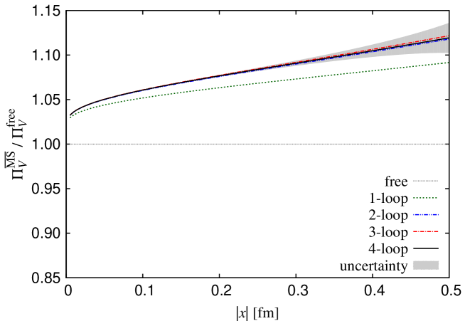
As shown in Fig. 4, the choice of μx,optsuperscriptsubscript𝜇𝑥opt\mu_{x}^{\rm*,opt} shows better convergence. The gray region in the figure represents the higher order uncertainty, which is estimated by the maximum difference between the correlator at μx=μx,optsuperscriptsubscript𝜇𝑥superscriptsubscript𝜇𝑥opt\mu_{x}^{*}=\mu_{x}^{*,\rm opt} and those at μxsuperscriptsubscript𝜇𝑥\mu_{x}^{*} in [12μx,opt,2μx,opt]12superscriptsubscript𝜇𝑥opt2superscriptsubscript𝜇𝑥opt[{1\over 2}\mu_{x}^{*,\rm opt},2\mu_{x}^{\rm*,opt}].

Refer to caption
Figure 4: Perturbative expansion of the vector correlator renormalized in the MS¯¯MS\rm\overline{MS} scheme with nf=3subscript𝑛𝑓3n_{f}=3. The results of the perturbative series (11) at the optimal scale μx=μx,optsuperscriptsubscript𝜇𝑥superscriptsubscript𝜇𝑥opt\mu_{x}^{*}=\mu_{x}^{\rm*,opt} truncated at as0superscriptsubscript𝑎𝑠0a_{s}^{0} (fine-dotted), assubscript𝑎𝑠a_{s} (dotted), as2superscriptsubscript𝑎𝑠2a_{s}^{2} (dashed double-dotted), as3superscriptsubscript𝑎𝑠3a_{s}^{3} (dashed dotted), and as4superscriptsubscript𝑎𝑠4a_{s}^{4} (solid) are plotted as functions of |x|𝑥|x|.

Next, we consider the scalar correlator. The scalar channel is more complicated due to the scale dependence of the scalar operator S(x)𝑆𝑥S(x). Using the beta function vanRitbergen:1997va and the anomalous dimension Chetyrkin:1997dh ; Vermaseren:1997fq , we can treat a general expression of the perturbative expansion of the scalar correlator, which is written as

ΠSMS¯(μx;x)=3π4x6(1+i=1CiS(μx,μx)as(μx)i),superscriptsubscriptΠ𝑆¯MSsuperscriptsubscript𝜇𝑥𝑥3superscript𝜋4superscript𝑥61superscriptsubscript𝑖1superscriptsubscript𝐶𝑖𝑆superscriptsubscript𝜇𝑥superscriptsubscript𝜇𝑥subscript𝑎𝑠superscriptsubscriptsuperscript𝜇𝑥𝑖\Pi_{S}^{\rm\overline{MS}}(\mu_{x}^{\prime};x)={3\over\pi^{4}x^{6}}\left(1+\sum_{i=1}^{\infty}C_{i}^{S}(\mu_{x}^{*},\mu_{x}^{\prime})a_{s}(\mu^{*}_{x})^{i}\right), (12)

where the first argument μxsuperscriptsubscript𝜇𝑥\mu_{x}^{*} of the perturbative coefficients is the renormalization scale of the strong coupling constant in the perturbative series and the second μxsuperscriptsubscript𝜇𝑥\mu_{x}^{\prime} is the renormalization scale of the scalar operator. Chetyrkin and Maier Chetyrkin:2010dx gave the perturbative coefficients of correlators at the renormalization scale μx=μx=μ~xsuperscriptsubscript𝜇𝑥superscriptsubscript𝜇𝑥subscript~𝜇𝑥\mu_{x}^{*}=\mu_{x}^{\prime}=\tilde{\mu}_{x}, which is CiS(μ~x,μ~x)superscriptsubscript𝐶𝑖𝑆subscript~𝜇𝑥subscript~𝜇𝑥C_{i}^{S}(\tilde{\mu}_{x},\tilde{\mu}_{x}) in our notation. The coefficients CiS(μx,μx)superscriptsubscript𝐶𝑖𝑆subscript𝜇𝑥subscript𝜇𝑥C_{i}^{S}(\mu_{x},\mu_{x}) and CiS(μ~x,μ~x)superscriptsubscript𝐶𝑖𝑆subscript~𝜇𝑥subscript~𝜇𝑥C_{i}^{S}(\tilde{\mu}_{x},\tilde{\mu}_{x}) are summarized in Appendix A.

Refer to caption
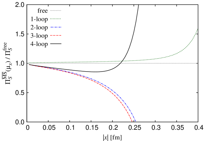
Figure 5: Scalar correlator renormalized at μxsubscript𝜇𝑥\mu_{x} in MS¯¯MS\rm\overline{MS} scheme for nf=3subscript𝑛𝑓3n_{f}=3. The results at μx=μx=μxsuperscriptsubscript𝜇𝑥superscriptsubscript𝜇𝑥subscript𝜇𝑥\mu_{x}^{*}=\mu_{x}^{\prime}=\mu_{x} truncated at as0superscriptsubscript𝑎𝑠0a_{s}^{0} (fine-dotted), assubscript𝑎𝑠a_{s} (dotted), as2superscriptsubscript𝑎𝑠2a_{s}^{2} (dashed double-dotted), as3superscriptsubscript𝑎𝑠3a_{s}^{3} (dashed dotted), and as4superscriptsubscript𝑎𝑠4a_{s}^{4} (solid) are plotted.
Refer to caption
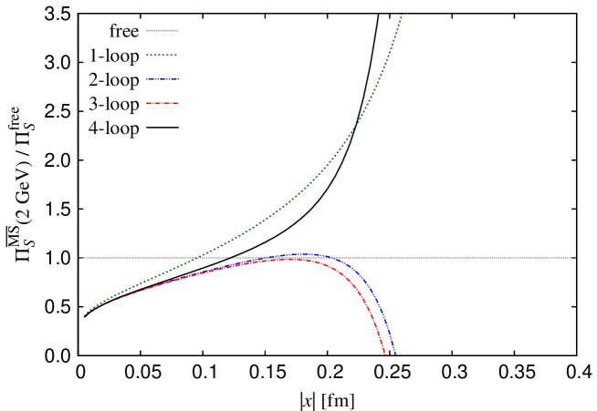
Figure 6: Scalar correlator renormalized at 2 GeV in MS¯¯MS\rm\overline{MS} scheme for nf=3subscript𝑛𝑓3n_{f}=3, which is calculated from the perturbative series at μx=μx=μxsuperscriptsubscript𝜇𝑥superscriptsubscript𝜇𝑥subscript𝜇𝑥\mu_{x}^{*}=\mu_{x}^{\prime}=\mu_{x} and the scale evolution. The results truncated at as0superscriptsubscript𝑎𝑠0a_{s}^{0} (fine-dotted), assubscript𝑎𝑠a_{s} (dotted), as2superscriptsubscript𝑎𝑠2a_{s}^{2} (dashed double-dotted), as3superscriptsubscript𝑎𝑠3a_{s}^{3} (dashed dotted), and as4superscriptsubscript𝑎𝑠4a_{s}^{4} (solid) are plotted.

Figure 6 shows the convergence of the perturbative expansion at μx=μx=μxsuperscriptsubscript𝜇𝑥superscriptsubscript𝜇𝑥subscript𝜇𝑥\mu_{x}^{*}=\mu_{x}^{\prime}=\mu_{x} with nf=3subscript𝑛𝑓3n_{f}=3. The correlator in the figure is normalized by the tree-level one, ΠSfree(x)=3/π4x6superscriptsubscriptΠ𝑆free𝑥3superscript𝜋4superscript𝑥6\Pi_{S}^{\rm free}(x)=3/\pi^{4}x^{6}. The scalar channel also shows poor convergence. The BLM scale is not directly applicable for scale dependent quantities. In fact, the BLM scale of the scalar correlator renormalized at μxsubscript𝜇𝑥\mu_{x} is unstable, i.e. μxBLM8.8μxsimilar-to-or-equalssuperscriptsubscript𝜇𝑥BLM8.8subscript𝜇𝑥\mu_{x}^{\rm BLM}\simeq 8.8\mu_{x} for ΠSMS¯(μ~x;x)superscriptsubscriptΠ𝑆¯MSsubscript~𝜇𝑥𝑥\Pi_{S}^{\rm\overline{MS}}(\tilde{\mu}_{x};x) while μxBLM4×103μxsimilar-to-or-equalssuperscriptsubscript𝜇𝑥BLM4superscript103subscript𝜇𝑥\mu_{x}^{\rm BLM}\simeq 4\times 10^{3}\mu_{x} for ΠSMS¯(μx;x)superscriptsubscriptΠ𝑆¯MSsubscript𝜇𝑥𝑥\Pi_{S}^{\rm\overline{MS}}(\mu_{x};x).

Since the purpose of this work is to determine the renormalization constant at 2 GeV in the MS¯¯MS\rm\overline{MS} scheme, we perform the scale evolution of the scalar correlator (12) from μxsuperscriptsubscript𝜇𝑥\mu_{x}^{\prime} to 2 GeV by a numerical integral of the mass anomalous dimension Chetyrkin:1997dh ; Vermaseren:1997fq . Figure 6 shows the scalar correlator calculated from the perturbative series at μx=μx=μxsuperscriptsubscript𝜇𝑥superscriptsubscript𝜇𝑥subscript𝜇𝑥\mu_{x}^{*}=\mu_{x}^{\prime}=\mu_{x} and the scale evolution with nf=3subscript𝑛𝑓3n_{f}=3. This calculation is convergent only below |x|0.06similar-to𝑥0.06|x|\sim 0.06 fm.

Refer to caption

Refer to caption

Refer to caption

Refer to caption

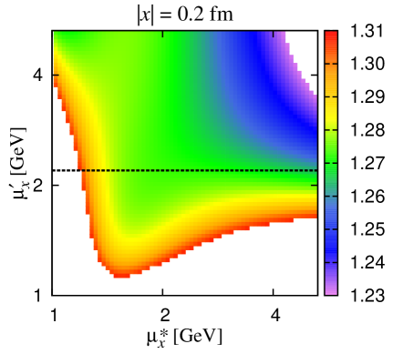
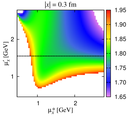
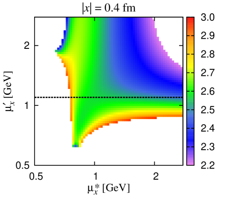
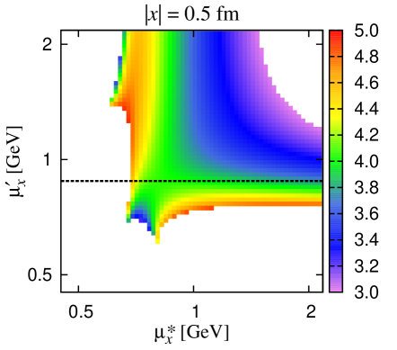
Figure 7: ΠSMS¯(2GeV;x)/ΠSfree(x)superscriptsubscriptΠ𝑆¯MS2GeV𝑥superscriptsubscriptΠ𝑆free𝑥\Pi_{S}^{\rm\overline{MS}}(2{\rm\ GeV};x)/\Pi_{S}^{\rm free}(x) at the four-loop level at nf=3subscript𝑛𝑓3n_{f}=3. The results at the specific distances 0.2 fm (top/left), 0.3 fm (top/right), 0.4 fm (bottom/left), and 0.5 fm (bottom/right) are shown as functions of μxsubscriptsuperscript𝜇𝑥\mu^{*}_{x} and μxsubscriptsuperscript𝜇𝑥\mu^{\prime}_{x}. The dashed lines stand for our choice of μxsuperscriptsubscript𝜇𝑥\mu_{x}^{\prime}, where the correlator shows small sensitivity to μxsubscriptsuperscript𝜇𝑥\mu^{\prime}_{x} and μxsuperscriptsubscript𝜇𝑥\mu_{x}^{*}.

Although the scalar correlator ΠSMS¯(2GeV;x)superscriptsubscriptΠ𝑆¯MS2GeV𝑥\Pi_{S}^{\rm\overline{MS}}({2\rm\ GeV};x) after the scale evolution has to be independent of both the scales μxsubscriptsuperscript𝜇𝑥\mu^{*}_{x} and μxsubscriptsuperscript𝜇𝑥\mu^{\prime}_{x}, finite order calculations may depend on them. Figure 7 shows the dependences on μxsuperscriptsubscript𝜇𝑥\mu_{x}^{*} and μxsuperscriptsubscript𝜇𝑥\mu_{x}^{\prime} of the four-loop results with nf=3subscript𝑛𝑓3n_{f}=3 at four representative distances renormalized at 2 GeV in the MS¯¯MS\rm\overline{MS} scheme. To choose optimal values of μxsuperscriptsubscript𝜇𝑥\mu_{x}^{*} and μxsuperscriptsubscript𝜇𝑥\mu_{x}^{\prime}, we focus on the region with mild dependence of the correlator. We choose the optimal values of μx(=μxopt)annotatedsubscriptsuperscript𝜇𝑥absentsuperscriptsubscript𝜇𝑥opt\mu^{\prime}_{x}(=\mu_{x}^{\prime\rm\ opt}) as indicated by the dashed lines in Fig. 7. On these lines, the correlator depends on μxsuperscriptsubscript𝜇𝑥\mu_{x}^{*} mildly and the dependence on μxsuperscriptsubscript𝜇𝑥\mu_{x}^{\prime} is also relatively small. Numerically, the choice is

μxopt=e0.8μx2.2x.superscriptsubscript𝜇𝑥optsuperscripte0.8subscript𝜇𝑥similar-to-or-equals2.2𝑥\mu_{x}^{\prime\rm\ opt}={\rm{e}}^{0.8}\mu_{x}\simeq{2.2\over x}. (13)

Refer to caption

Refer to caption

Refer to caption

Refer to caption

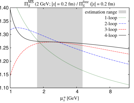
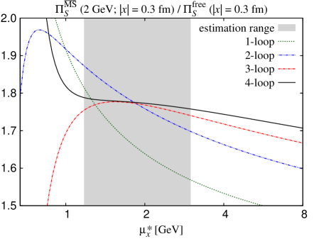
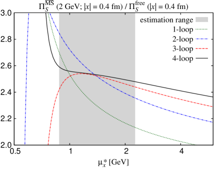
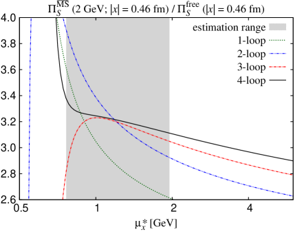
Figure 8: Scalar correlator renormalized at 2 GeV in the MS¯¯MS\rm\overline{MS} scheme at the specific distances 0.2 fm (top/left), 0.3 fm (top/right), 0.4 fm (bottom/left), and 0.46 fm (bottom/right) as functions of μxsubscriptsuperscript𝜇𝑥\mu^{*}_{x}. They are calculated at nf=3subscript𝑛𝑓3n_{f}=3 and μxsuperscriptsubscript𝜇𝑥\mu_{x}^{\prime} is set by (13). The results truncated at assubscript𝑎𝑠a_{s} (dotted), as2superscriptsubscript𝑎𝑠2a_{s}^{2} (dashed double-dotted), as3superscriptsubscript𝑎𝑠3a_{s}^{3} (dashed dotted), and as4superscriptsubscript𝑎𝑠4a_{s}^{4} (solid) are plotted. The gray band represents the region in which we estimate the uncertainty of the perturbative calculation.

The detailed dependence of the scalar correlator on μxsuperscriptsubscript𝜇𝑥\mu_{x}^{*} at μx=μxoptsuperscriptsubscript𝜇𝑥superscriptsubscript𝜇𝑥opt\mu_{x}^{\prime}=\mu_{x}^{\prime\rm\ opt} is shown in Fig. 8 for several distances in 0.2–0.46 fm, in which we determine the renormalization factor of the scalar operator. These figures show results at each loop order up to the four-loop level. We then choose the optimal value μx,optsuperscriptsubscript𝜇𝑥opt\mu_{x}^{*,\rm opt} of the scale μxsuperscriptsubscript𝜇𝑥\mu_{x}^{*} as the value which minimizes the dependence on μxsuperscriptsubscript𝜇𝑥\mu_{x}^{*},

μx,opt=e1.05μx2.9x.superscriptsubscript𝜇𝑥optsuperscripte1.05subscript𝜇𝑥similar-to-or-equals2.9𝑥\mu_{x}^{*,\rm opt}={\rm{e}}^{1.05}\mu_{x}\simeq{2.9\over x}. (14)

We estimate the uncertainty by varying μxsubscriptsuperscript𝜇𝑥\mu^{*}_{x} in a region including μx,optsuperscriptsubscript𝜇𝑥opt\mu_{x}^{*,\rm opt} in the middle as we did for the vector channel. Since the coupling constant blows up as μxsuperscriptsubscript𝜇𝑥\mu_{x}^{*} approaches ΛQCDsubscriptΛQCD\Lambda_{\rm QCD}, we need to avoid too small μxsuperscriptsubscript𝜇𝑥\mu_{x}^{*}. Therefore, our choice is [11.6μx,opt,1.6μx,opt]11.6superscriptsubscript𝜇𝑥opt1.6superscriptsubscript𝜇𝑥opt[{1\over 1.6}\mu_{x}^{*,\rm opt},1.6\mu_{x}^{*,\rm opt}] in order not to use the coupling constant at the scale smaller than 0.750.750.75 GeV. The region is shown by the gray band in Fig. 8.
Refer to caption
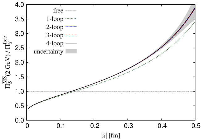
Figure 9: Scalar correlator renormalized at 2 GeV in the MS¯¯MS\rm\overline{MS} scheme at nf=3subscript𝑛𝑓3n_{f}=3. The scale parameters μxsuperscriptsubscript𝜇𝑥\mu_{x}^{\prime} and μxsuperscriptsubscript𝜇𝑥\mu_{x}^{*} are set by (13) and (14). The results truncated at as0superscriptsubscript𝑎𝑠0a_{s}^{0} (fine-dotted), assubscript𝑎𝑠a_{s} (dotted), as2superscriptsubscript𝑎𝑠2a_{s}^{2} (dashed double-dotted), as3superscriptsubscript𝑎𝑠3a_{s}^{3} (dashed dotted), and as4superscriptsubscript𝑎𝑠4a_{s}^{4} (solid) are plotted. The gray region stands for the uncertainty of higher order corrections, which is estimated by the sensitivity to μxsuperscriptsubscript𝜇𝑥\mu_{x}^{*}.

Setting μxsuperscriptsubscript𝜇𝑥\mu_{x}^{\prime} and μxsuperscriptsubscript𝜇𝑥\mu_{x}^{*} by (13) and (14), we obtain the following numerical expansion at nf=3subscript𝑛𝑓3n_{f}=3,

ΠSMS¯(μxopt;x)|nf=3=3π4x6(1\displaystyle\Pi_{S}^{\rm\overline{MS}}(\mu_{x}^{\prime\rm\ opt};x)\Big{|}_{n_{f}=3}={3\over\pi^{4}x^{6}}\Big{(}1 +3.4029as(μx,opt)+9.7142as(μx,opt)23.4029subscript𝑎𝑠superscriptsubscript𝜇𝑥opt9.7142subscript𝑎𝑠superscriptsuperscriptsubscript𝜇𝑥opt2\displaystyle+3.4029a_{s}(\mu_{x}^{*,\rm opt})+9.7142a_{s}(\mu_{x}^{*,\rm opt})^{2}
+1.7011as(μx,opt)3+26.366as(μx,opt)4+O(as5)).\displaystyle+1.7011a_{s}(\mu_{x}^{*,\rm opt})^{3}+26.366a_{s}(\mu_{x}^{*,\rm opt})^{4}+O(a_{s}^{5})\Big{)}. (15)

The four-loop correction in this series is much smaller than that 579as(μx)4similar-toabsent579subscript𝑎𝑠superscriptsubscript𝜇𝑥4\sim 579a_{s}(\mu_{x})^{4} in the perturbative series at μx=μxsuperscriptsubscript𝜇𝑥subscript𝜇𝑥\mu_{x}^{*}=\mu_{x} (see Appendix A), implying that the convergence of the perturbative series (15) is better than that at μx=μxsuperscriptsubscript𝜇𝑥subscript𝜇𝑥\mu_{x}^{*}=\mu_{x}. In fact, evolving the renormalization scale of the correlator to 2 GeV, we obtain a well convergent correlator as shown in Fig. 9. The figure also shows the uncertainty of the perturbative calculation by the gray band, which is estimated by the maximum difference between the correlator at μx=μx,optsuperscriptsubscript𝜇𝑥superscriptsubscript𝜇𝑥opt\mu_{x}^{*}=\mu_{x}^{*,\rm opt} and those at μxsuperscriptsubscript𝜇𝑥\mu_{x}^{*} in [11.6μx,opt,1.6μx,opt]11.6superscriptsubscript𝜇𝑥opt1.6superscriptsubscript𝜇𝑥opt[{1\over 1.6}\mu_{x}^{*,\rm opt},1.6\mu_{x}^{\rm*,opt}].

III.2 Operator Product Expansion

In the previous subsection, we discuss the correlators in perturbation theory. In the real QCD vacuum with the spontaneous breaking of chiral symmetry, however, additional terms with vacuum expectation values of operators may appear, inducing the violation of the degeneracy between the scalar and pseudoscalar, and between the vector and axial-vector channels.

In the momentum space, the Operator Product Expansion (OPE) of correlators is sketched as

Π~ΓOPE(q2)=Π~Γpert(q2)+𝒪c~𝒪Γ(q2)q2dim𝒪𝒪,superscriptsubscript~ΠΓOPEsuperscript𝑞2superscriptsubscript~ΠΓpertsuperscript𝑞2subscript𝒪superscriptsubscript~𝑐𝒪Γsuperscript𝑞2superscript𝑞2dimension𝒪delimited-⟨⟩𝒪\widetilde{\Pi}_{\Gamma}^{\rm OPE}(q^{2})=\widetilde{\Pi}_{\Gamma}^{\rm pert}(q^{2})+\sum_{\cal O}\tilde{c}_{\cal O}^{\Gamma}(q^{2})q^{2-\dim\cal O}\langle{\cal O}\rangle, (16)

where the first term on the RHS corresponds to the perturbative contribution including the quark mass corrections. Here 𝒪𝒪\cal O denotes operators with the mass dimension four and higher,

𝒪{mqq¯q,asG2,mqgsq¯Gq,as(q¯q)2,},𝒪subscript𝑚𝑞¯𝑞𝑞subscript𝑎𝑠superscript𝐺2subscript𝑚𝑞subscript𝑔𝑠¯𝑞𝐺𝑞subscript𝑎𝑠superscript¯𝑞𝑞2{\cal O}\in\{m_{q}\bar{q}q,a_{s}G^{2},m_{q}g_{s}\bar{q}Gq,a_{s}(\bar{q}q)^{2},\cdots\}, (17)

and the Wilson coefficients c~𝒪Γ(q2)superscriptsubscript~𝑐𝒪Γsuperscript𝑞2\tilde{c}_{\cal O}^{\Gamma}(q^{2}) do not have mass dimensions. In general, c~𝒪Γsuperscriptsubscript~𝑐𝒪Γ\widetilde{c}_{\cal O}^{\Gamma}’s depend on q2superscript𝑞2q^{2} logarithmically as ln(q2/μ2)superscript𝑞2superscript𝜇2\ln(q^{2}/\mu^{2}) and on the quark mass as mq2/q2superscriptsubscript𝑚𝑞2superscript𝑞2m_{q}^{2}/q^{2}. These coefficients are known up to dim𝒪=8dimension𝒪8\dim{\cal O}=8 Shifman:1978bx ; Broadhurst:1985js ; Jamin:1992se .

The short-distance behavior of the correlators in the coordinate space is obtained by Fourier transform

ΠΓOPE(x2)=d4q(2π)4eiqxΠ~ΓOPE(q2)=ΠΓpert(x2)+𝒪c𝒪Γ(x2)xdim𝒪6𝒪.superscriptsubscriptΠΓOPEsuperscript𝑥2superscriptd4𝑞superscript2𝜋4superscriptei𝑞𝑥superscriptsubscript~ΠΓOPEsuperscript𝑞2superscriptsubscriptΠΓpertsuperscript𝑥2subscript𝒪superscriptsubscript𝑐𝒪Γsuperscript𝑥2superscript𝑥dimension𝒪6delimited-⟨⟩𝒪\Pi_{\Gamma}^{\rm OPE}(x^{2})=\int{{\rm{d}}^{4}q\over(2\pi)^{4}}{\rm{e}}^{{\rm{i}}qx}\widetilde{\Pi}_{\Gamma}^{\rm OPE}(q^{2})=\Pi_{\Gamma}^{\rm pert}(x^{2})+\sum_{\cal O}c_{\cal O}^{\Gamma}(x^{2})x^{\dim{\cal O}-6}\langle{\cal O}\rangle. (18)

A convenient set of relations between the momentum space and the coordinate space is summarized in Narison:2001ix . Using these relations, we obtain the Wilson coefficients in the coordinate space:

cmq¯qS/P=1±24π2+O(as,mq2x2),cmq¯qV/A=142π2+O(as,mq2x2),formulae-sequencesuperscriptsubscript𝑐𝑚¯𝑞𝑞𝑆𝑃plus-or-minus124superscript𝜋2𝑂subscript𝑎𝑠superscriptsubscript𝑚𝑞2superscript𝑥2superscriptsubscript𝑐𝑚¯𝑞𝑞𝑉𝐴minus-or-plus142superscript𝜋2𝑂subscript𝑎𝑠superscriptsubscript𝑚𝑞2superscript𝑥2\displaystyle c_{m\bar{q}q}^{S/P}={1\pm 2\over 4\pi^{2}}+O(a_{s},m_{q}^{2}x^{2}),\ \ c_{m\bar{q}q}^{V/A}={1\mp 4\over 2\pi^{2}}+O(a_{s},m_{q}^{2}x^{2}), (19)
casG2S/P=132π2+O(as,mq2x2),casG2V/A=116π2+O(as,mq2x2),formulae-sequencesuperscriptsubscript𝑐subscript𝑎𝑠superscript𝐺2𝑆𝑃132superscript𝜋2𝑂subscript𝑎𝑠superscriptsubscript𝑚𝑞2superscript𝑥2superscriptsubscript𝑐subscript𝑎𝑠superscript𝐺2𝑉𝐴116superscript𝜋2𝑂subscript𝑎𝑠superscriptsubscript𝑚𝑞2superscript𝑥2\displaystyle c_{a_{s}G^{2}}^{S/P}={1\over 32\pi^{2}}+O(a_{s},m_{q}^{2}x^{2}),\ \ c_{a_{s}G^{2}}^{V/A}=-{1\over 16\pi^{2}}+O(a_{s},m_{q}^{2}x^{2}), (20)
cmgsq¯GqS/P=116π2ln(x/x0)2+O(as,mq2x2),cmgsq¯GqV/A=0,\displaystyle c_{mg_{s}\bar{q}Gq}^{S/P}=\mp{1\over 16\pi^{2}}\ln(x/x_{0})^{2}+O(a_{s},m_{q}^{2}x^{2}),\ \ c_{mg_{s}\bar{q}Gq}^{V/A}=0, (21)
cas(q¯q)2S/P=4±1127ln(x/x0)2+O(as,mq2x2),cas(q¯q)2V/A=2(29)27ln(x/x0)2+O(as,mq2x2).\displaystyle c_{a_{s}(\bar{q}q)^{2}}^{S/P}={4\pm 11\over 27}\ln(x/x_{0})^{2}+O(a_{s},m_{q}^{2}x^{2}),\ \ c_{a_{s}(\bar{q}q)^{2}}^{V/A}={2(2\mp 9)\over 27}\ln(x/x_{0})^{2}+O(a_{s},m_{q}^{2}x^{2}). (22)

Here, the coefficients of the four-quark condensate cas(q¯q)2Γsuperscriptsubscript𝑐subscript𝑎𝑠superscript¯𝑞𝑞2Γc_{a_{s}(\bar{q}q)^{2}}^{\Gamma} are calculated using the vacuum saturation approximation Narison:2001ix . The logarithmic contributions in (21) and (22) involve dimensionful variable x0subscript𝑥0x_{0}, which appears from divergences of the integral defining the Fourier transform and are regularization and scheme dependent.

The perturbative contribution on the RHS of (18) also includes the mass term which also violates the degeneracy of the scalar and pseudoscalar, or the vector and axial-vector channels. The massless part is already discussed in the previous subsection. The mass term contributes as

ΠP/Spert(x2)ΠP/Spert,massless(x2)superscriptsubscriptΠ𝑃𝑆pertsuperscript𝑥2superscriptsubscriptΠ𝑃𝑆pertmasslesssuperscript𝑥2\displaystyle\Pi_{P/S}^{\rm pert}(x^{2})-\Pi_{P/S}^{\rm pert,massless}(x^{2}) =3(2±1)mq24π4x4+O(αs/π,mq4/x2),absent3plus-or-minus21superscriptsubscript𝑚𝑞24superscript𝜋4superscript𝑥4𝑂subscript𝛼𝑠𝜋superscriptsubscript𝑚𝑞4superscript𝑥2\displaystyle=-{3(2\pm 1)m_{q}^{2}\over 4\pi^{4}x^{4}}+O(\alpha_{s}/\pi,m_{q}^{4}/x^{2}), (23)
ΠV/Apert(x2)ΠV/Apert,massless(x2)superscriptsubscriptΠ𝑉𝐴pertsuperscript𝑥2superscriptsubscriptΠ𝑉𝐴pertmasslesssuperscript𝑥2\displaystyle\Pi_{V/A}^{\rm pert}(x^{2})-\Pi_{V/A}^{\rm pert,massless}(x^{2}) =6(11)mq2π4x4+O(αs/π,mq4/x2).absent6minus-or-plus11superscriptsubscript𝑚𝑞2superscript𝜋4superscript𝑥4𝑂subscript𝛼𝑠𝜋superscriptsubscript𝑚𝑞4superscript𝑥2\displaystyle=-{6(1\mp 1)m_{q}^{2}\over\pi^{4}x^{4}}+O(\alpha_{s}/\pi,m_{q}^{4}/x^{2}). (24)

In the renormalization condition (5), we add these mass correction terms to ΠΓMS¯(2GeV;x)superscriptsubscriptΠΓ¯MS2GeV𝑥\Pi_{\Gamma}^{\rm\overline{MS}}({2\rm\ GeV};x).

IV Lattice calculation

IV.1 Lattice Setup

Table 1: Lattice ensembles used in this work.
β𝛽\beta a𝑎a [fm] Ns3×Nt×Lssuperscriptsubscript𝑁𝑠3subscript𝑁𝑡subscript𝐿𝑠N_{s}^{3}\times N_{t}\times L_{s} ams𝑎subscript𝑚𝑠am_{s} amq𝑎subscript𝑚𝑞am_{q} aMπ𝑎subscript𝑀𝜋aM_{\pi} Nconfsubscript𝑁confN_{\rm conf} Nsrcsubscript𝑁srcN_{\rm src}
4.17 0.0804 323×64×12superscript323641232^{3}\times 64\times 12 0.0300 0.0070 0.1263(4) 200 4
0.0120 0.1618(3) 200 2
0.0190 0.2030(3) 200 2
483×96×12superscript483961248^{3}\times 96\times 12 0.0400 0.0035 0.0921(1) 200 2
323×64×12superscript323641232^{3}\times 64\times 12 0.0070 0.1260(4) 200 4
0.0120 0.1627(3) 200 2
0.0190 0.2033(3) 200 2
4.35 0.0547 483×96×8superscript48396848^{3}\times 96\times 8 0.0180 0.0042 0.0820(3) 200 2
0.0080 0.1127(3) 200 1
0.0120 0.1381(3) 200 1
0.0250 0.0042 0.0831(4) 200 2
0.0080 0.1130(3) 200 1
0.0120 0.1387(3) 200 1
4.47 0.0439 643×128×8superscript643128864^{3}\times 128\times 8 0.0150 0.0030 0.0632(2) 200 1

In this work, we perform lattice simulations with 2+1212+1-flavor dynamical Möbius domain-wall fermions Brower:2004xi ; Brower:2012vk with three-step stout link smearing Morningstar:2003gk and the tree-level Symanzik improved gauge action Luscher:1984xn . The properties of the gauge ensembles used in this analysis are summarized in Table 1. The input strange quark mass mssubscript𝑚𝑠m_{s} is only for the sea quark, while the mass mqsubscript𝑚𝑞m_{q} of two degenerate quarks, up and down, is used for both the valence and sea quarks. The computed pion masses Mπsubscript𝑀𝜋M_{\pi} are in the region 230–500 MeV.

For each ensemble, Nconf=200subscript𝑁conf200N_{\rm conf}=200 configurations are sampled from 10,000 molecular dynamics time. For each configuration, we calculate correlators from one or more (Nsrcsubscript𝑁srcN_{\rm src}) source points. We use the IroIro++++ simulation code Cossu:2013ola for these calculations.

Considering the violation of rotational symmetry, we distinguish different lattice points that are not related by 90superscript9090^{\circ} rotations in the four-dimensional cubic group and average the correlators on the lattice over the lattice points that are related by 90superscript9090^{\circ} rotations. We then have 322 sets of different separations in the region 1(x/a)21001superscript𝑥𝑎21001\leq(x/a)^{2}\leq 100.

IV.2 Reduction of discretization effect
Refer to caption
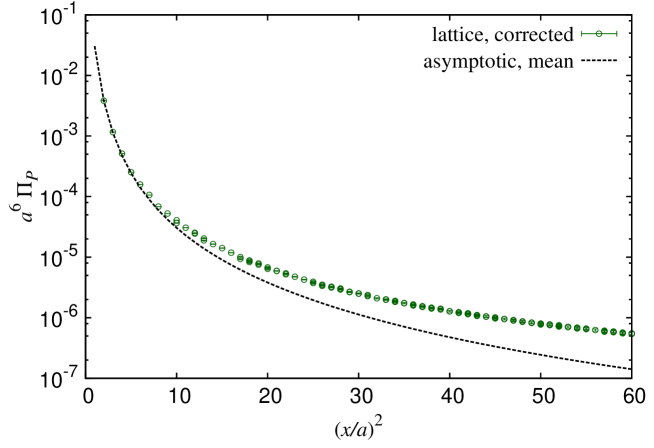
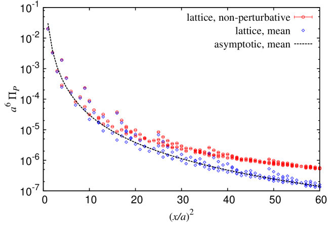
Figure 10: Pseudoscalar correlator obtained by the lattice calculation (circles) and its mean field approximation (diamonds) at the same valence mass. The dashed curve represents the asymptotic behavior of the mean field approximation. The lattice data on the 483×96superscript4839648^{3}\times 96 at β=4.35𝛽4.35\beta=4.35 and (amq,ams)=(0.0042,0.0180)𝑎subscript𝑚𝑞𝑎subscript𝑚𝑠0.00420.0180(am_{q},am_{s})=(0.0042,0.0180) are plotted as a representative.
Refer to caption
Figure 11: Pseudoscalar correlator after applying the subtraction (25). The result on the same ensemble as in Fig. 11 is shown.

The pseudoscalar correlator ΠPlat(x)superscriptsubscriptΠ𝑃lat𝑥\Pi_{P}^{\rm lat}(x) calculated non-perturbatively on the ensemble at β=4.35,(amq,ams)=(0.0042,0.0180)formulae-sequence𝛽4.35𝑎subscript𝑚𝑞𝑎subscript𝑚𝑠0.00420.0180\beta=4.35,(am_{q},am_{s})=(0.0042,0.0180) is plotted in Fig. 11. This figure also shows the mean field approximation ΠPlat,mean(x)superscriptsubscriptΠ𝑃latmean𝑥\Pi_{P}^{\rm lat,mean}(x) of the pseudoscalar correlator on the lattice and its asymptotic form ΠPasym,mean(x)superscriptsubscriptΠ𝑃asymmean𝑥\Pi_{P}^{\rm asym,mean}(x) in the long-distance limit. The mean field approximation on the lattice is calculated by a contraction of the propagators of the domain-wall fermions in the mean field theory and its long-distance limit is calculated by applying Taylor expansion (see Appendix B for more detail).

The non-perturbative lattice data are not on a smooth curve due to discretization effects. However, the similar discretization effect as seen in the free theory as well as in the mean field approximation describes the bulk of the discretization effects. We therefore improve the lattice data by applying a subtraction,

ΠΓlat(x)ΠΓlat(x)(ΠΓlat,mean(x)ΠΓasym,mean(x)).superscriptsubscriptΠΓlat𝑥superscriptsubscriptΠΓlat𝑥superscriptsubscriptΠΓlatmean𝑥superscriptsubscriptΠΓasymmean𝑥\Pi_{\Gamma}^{\rm lat}(x)\rightarrow\Pi_{\Gamma}^{\rm lat}(x)-\big{(}\Pi_{\Gamma}^{\rm lat,mean}(x)-\Pi_{\Gamma}^{\rm asym,mean}(x)\big{)}. (25)

As shown in Fig. 11, we obtain much smoother correlators.
Refer to caption
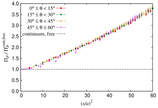
Figure 12: Pseudoscalar correlator divided by the tree-level continuum correlator after applying the subtraction (25). The data in 0θ<15superscript0𝜃superscript150^{\circ}\leq\theta<15^{\circ} (circles), 15θ<30superscript15𝜃superscript3015^{\circ}\leq\theta<30^{\circ} (diamonds), 30θ<45superscript30𝜃superscript4530^{\circ}\leq\theta<45^{\circ} (squares), and 45θ60superscript45𝜃superscript6045^{\circ}\leq\theta\leq 60^{\circ} (pentagons) are separately plotted. The result on the same ensemble as in Fig. 11 is shown.
Refer to caption
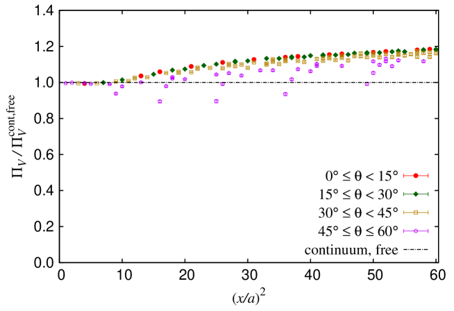
Figure 13: Same as Fig. 13 but for the vector channel.
Refer to caption
Figure 14: Detailed view of Fig. 13. The Data in 0θ<20superscript0𝜃superscript200^{\circ}\leq\theta<20^{\circ} (circles), 20θ<30superscript20𝜃superscript3020^{\circ}\leq\theta<30^{\circ} (diamonds), and at θ=30𝜃superscript30\theta=30^{\circ} (crosses) are separately plotted. Data at θ>30𝜃superscript30\theta>30^{\circ} are omitted.

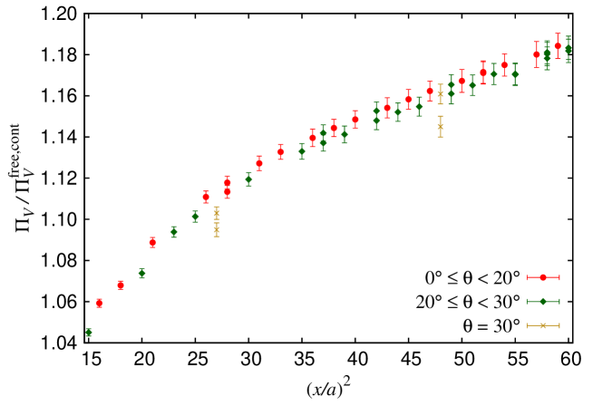
Figures 13 and 13 show the pseudoscalar and vector correlators, respectively, after applying the subtraction (25). They are normalized by the continuum free correlator ΠP/Vcont,free(x)superscriptsubscriptΠ𝑃𝑉contfree𝑥\Pi_{P/V}^{\rm cont,free}(x) and plotted in a linear scale. Here, we introduce a parameter θ𝜃\theta, which is defined as an angle between the four-dimensional point x𝑥x and the direction (1,1,1,1)1111(1,1,1,1). In four-dimension, θ𝜃\theta is not larger than 60superscript6060^{\circ}. This parameter is strongly correlated with the discretization effects as discussed in Chu:1993cn ; Cichy:2012is , i.e. the discretization effects increase as θ𝜃\theta increases. It is observed even after applying the subtraction (25).

As seen in Fig. 14, which is a magnification of Fig. 13 in the range 0θ30superscript0𝜃superscript300^{\circ}\leq\theta\leq 30^{\circ}, there are discretization effects visible already at θ=30𝜃superscript30\theta=30^{\circ}. Although the points (0,3,3,3) and (1,1,3,4) are both at (x/a)2=27superscript𝑥𝑎227(x/a)^{2}=27 and θ=30𝜃superscript30\theta=30^{\circ}, the values disagree beyond the statistical error. The same is observed for the data at (0,4,4,4) and (2,2,2,6) sharing (x/a)2=48superscript𝑥𝑎248(x/a)^{2}=48 and θ=30𝜃superscript30\theta=30^{\circ}. The similar situation occurs more frequently for θ>30𝜃superscript30\theta>30^{\circ}. Namely, the data in the region θ30𝜃superscript30\theta\geq 30^{\circ} cannot be simply parametrized by any functions of θ𝜃\theta, and we therefore omit them in the analysis. Figure 14 also indicates that the lattice data at θ<30𝜃superscript30\theta<30^{\circ} may slightly depend on θ𝜃\theta. For the determination of the renormalization factor in the next section, we separately treat the discretization effects at θ<20𝜃superscript20\theta<20^{\circ} and at θ20𝜃superscript20\theta\geq 20^{\circ}.

IV.3 Subtraction of finite volume effect

Point-to-point correlators may contain finite volume effect, which relates correlators ΠΓL3×T(x)superscriptsubscriptΠΓsuperscript𝐿3𝑇𝑥\Pi_{\Gamma}^{L^{3}\times T}(x) in a finite volume with periodic boundaries to those ΠΓ(x)superscriptsubscriptΠΓ𝑥\Pi_{\Gamma}^{\infty}(x) in the infinite volume as

ΠΓL3×T(x)=ΠΓ(x)+x0ΠΓ(xx0),superscriptsubscriptΠΓsuperscript𝐿3𝑇𝑥superscriptsubscriptΠΓ𝑥subscriptsubscript𝑥0superscriptsubscriptΠΓ𝑥subscript𝑥0\Pi_{\Gamma}^{L^{3}\times T}(x)=\Pi_{\Gamma}^{\infty}(x)+\sum_{x_{0}}\Pi_{\Gamma}^{\infty}(x-x_{0}), (26)

where the sum over x0subscript𝑥0x_{0} runs over

x0{(±L,0,0,0),(0,±L,0,0),(0,0,±L,0),(0,0,0,±T),(±L,±L,0,0),}.subscript𝑥0plus-or-minus𝐿0000plus-or-minus𝐿0000plus-or-minus𝐿0000plus-or-minus𝑇plus-or-minus𝐿plus-or-minus𝐿00x_{0}\in\{(\pm L,0,0,0),(0,\pm L,0,0),(0,0,\pm L,0),(0,0,0,\pm T),(\pm L,\pm L,0,0),\cdots\}. (27)

Since the pseudoscalar correlator is expected to contain large finite volume effects due to the pion pole, we focus on this channel. The second term on the RHS of (26) is then dominated by the contribution of pion, which is well approximated using the modified Bessel function K1subscript𝐾1K_{1}. We apply the subtraction

ΠP(x)=ΠPL3×T(x)z0Mπ22π2x0K1(Mπ|xx0|)|xx0|,superscriptsubscriptΠ𝑃𝑥superscriptsubscriptΠ𝑃superscript𝐿3𝑇𝑥subscript𝑧0superscriptsubscript𝑀𝜋22superscript𝜋2subscriptsubscript𝑥0subscript𝐾1subscript𝑀𝜋𝑥subscript𝑥0𝑥subscript𝑥0\Pi_{P}^{\infty}(x)=\Pi_{P}^{L^{3}\times T}(x)-{z_{0}M_{\pi}^{2}\over 2\pi^{2}}\sum_{x_{0}}{K_{1}(M_{\pi}|x-x_{0}|)\over|x-x_{0}|}, (28)

where Mπsubscript𝑀𝜋M_{\pi} and z0subscript𝑧0z_{0} are extracted from the asymptotic form of the zero-momentum correlator, d3xΠP(x,t)z0eMπtsuperscriptd3𝑥subscriptΠ𝑃𝑥𝑡subscript𝑧0superscriptesubscript𝑀𝜋𝑡\int{\rm{d}}^{3}x\Pi_{P}(\vec{x},t)\rightarrow z_{0}{\rm{e}}^{-M_{\pi}t}.

Refer to caption
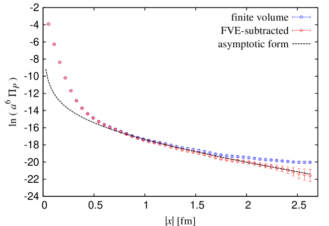
Figure 15: Pseudoscalar correlator in the time-direction (|x|=t𝑥𝑡|x|=t) before (circles) and after (diamonds) applying the subtraction (28). Dashed curve corresponds to the asymptotic form obtained by analyzing the zero momentum correlator. Data on the same ensemble as in Fig. 11 are plotted.

Figure 15 shows the pseudoscalar correlator before and after applying the subtraction (28) of the finite volume effects. The correlators only on the time axis (0,t(=|x|))0annotated𝑡absent𝑥(\vec{0},t(=|x|)) are plotted. We observe that the correlator after applying the subtraction (28) becomes consistent with the asymptotic form (dashed curve) at long distances.
Refer to caption
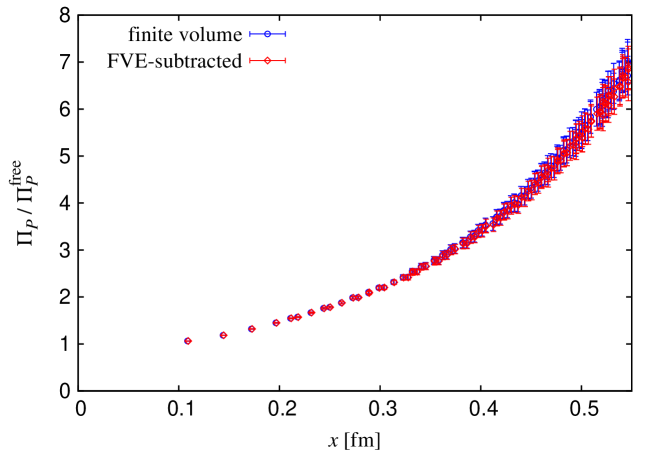
Figure 16: Pseudoscalar correlator before (circles) and after (diamonds) applying the subtraction (28). Data on the same ensemble as in Fig. 11 are plotted.

From Fig. 15, we find that the finite volume effects are significant at x1greater-than-or-equivalent-to𝑥1x\gtrsim 1 fm. In Fig. 16, we compare ΠP(x)/ΠPfree(x)subscriptΠ𝑃𝑥superscriptsubscriptΠ𝑃free𝑥\Pi_{P}(x)/\Pi_{P}^{\rm free}(x) before and after the subtraction (28) in the short distances x0.5less-than-or-similar-to𝑥0.5x\lesssim 0.5 fm and find that the magnitude of the finite volume effect in the pseudoscalar correlator at the short distances is less than 20% of the statistical errors. Since the finite volume effects are already small in the pseudoscalar correlator, those in other channels are expected to be negligible. In this work, we apply the subtraction (28) only for the pseudoscalar channel.

V Determination of renormalization constants

V.1 Determination of ZVsubscript𝑍𝑉Z_{V}

With domain-wall fermions that precisely satisfies the Ginsparg-Wilson relation, the identity ZVMS¯/lat(a)=ZAMS¯/lat(a)superscriptsubscript𝑍𝑉¯MSlat𝑎superscriptsubscript𝑍𝐴¯MSlat𝑎Z_{V}^{\rm\overline{MS}/lat}(a)=Z_{A}^{\rm\overline{MS}/lat}(a) is valid. In the analysis of ZVMS¯/lat(a)superscriptsubscript𝑍𝑉¯MSlat𝑎Z_{V}^{\rm\overline{MS}/lat}(a), the renormalization scale 2 GeV can be omitted because the current conservation ensures its scale independence.
Refer to caption
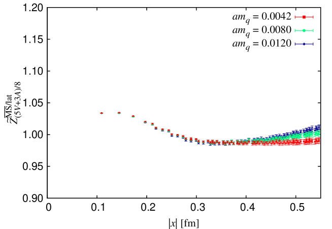
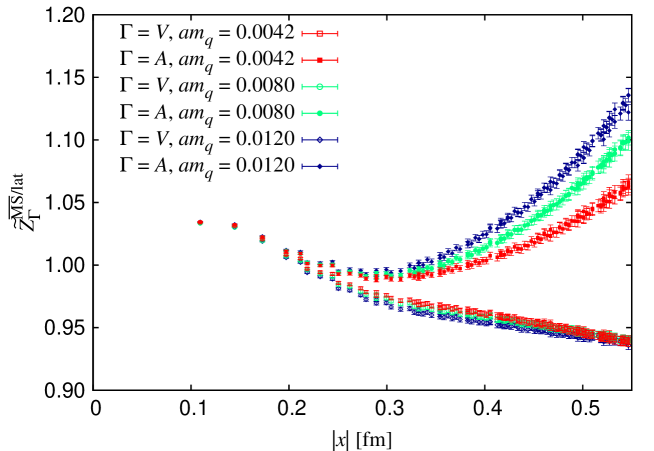
Figure 17: Z~VMS¯/lat(a;x)subscriptsuperscript~𝑍¯MSlat𝑉𝑎𝑥\widetilde{Z}^{\rm\overline{MS}/lat}_{V}(a;x) (open points) and Z~AMS¯/lat(a;x)superscriptsubscript~𝑍𝐴¯MSlat𝑎𝑥\widetilde{Z}_{A}^{\rm\overline{MS}/lat}(a;x) (filled points) calculated by (5) at the three input masses amq=0.0042𝑎subscript𝑚𝑞0.0042am_{q}=0.0042 (squares), 0.080 (circles), 0.0120 (diamonds) and β=4.35,ams=0.0180formulae-sequence𝛽4.35𝑎subscript𝑚𝑠0.0180\beta=4.35,am_{s}=0.0180.
Refer to caption
Figure 18: Z~(5V+3A)/8MS¯/lat(a;x)superscriptsubscript~𝑍5𝑉3𝐴8¯MSlat𝑎𝑥\widetilde{Z}_{(5V+3A)/8}^{\rm\overline{MS}/lat}(a;x) defined by (30). The results on the same ensembles as in Fig. 18 are shown.

Figure 18 shows x𝑥x-dependence of Z~VMS¯/lat(a;x)superscriptsubscript~𝑍𝑉¯MSlat𝑎𝑥\widetilde{Z}_{V}^{\rm\overline{MS}/lat}(a;x) and Z~AMS¯/lat(a;x)superscriptsubscript~𝑍𝐴¯MSlat𝑎𝑥\widetilde{Z}_{A}^{\rm\overline{MS}/lat}(a;x), which are defined by (5), at three input masses and β=4.35,ams=0.0180formulae-sequence𝛽4.35𝑎subscript𝑚𝑠0.0180\beta=4.35,am_{s}=0.0180. For |x|<0.2𝑥0.2|x|<0.2 fm, the results increase toward the short-distance regime due to the remnant discretization effects as discussed later. For |x|>0.25𝑥0.25|x|>0.25 fm, there is a significant splitting between the vector and axial-vector channels due to the non-perturbative effects.

The leading non-perturbative effect is described by OPE. According to the discussion in Section III.2, the coefficients c4,q¯qVsuperscriptsubscript𝑐4¯𝑞𝑞𝑉c_{4,\bar{q}q}^{V} and c4,q¯qAsuperscriptsubscript𝑐4¯𝑞𝑞𝐴c_{4,\bar{q}q}^{A} in the OPE of the vector and axial-vector correlators,

ΠV/A(x)=c0x6+c4,q¯qV/Amqq¯q+c4,GV/AGGx2+,subscriptΠ𝑉𝐴𝑥subscript𝑐0superscript𝑥6superscriptsubscript𝑐4¯𝑞𝑞𝑉𝐴subscript𝑚𝑞delimited-⟨⟩¯𝑞𝑞superscriptsubscript𝑐4𝐺𝑉𝐴delimited-⟨⟩𝐺𝐺superscript𝑥2\Pi_{V/A}(x)={c_{0}\over x^{6}}+{c_{4,\bar{q}q}^{V/A}m_{q}\langle\bar{q}q\rangle+c_{4,G}^{V/A}\langle GG\rangle\over x^{2}}+\cdots, (29)

satisfy c4,q¯qV/c4,q¯qA=3/5superscriptsubscript𝑐4¯𝑞𝑞𝑉superscriptsubscript𝑐4¯𝑞𝑞𝐴35c_{4,\bar{q}q}^{V}/c_{4,\bar{q}q}^{A}=-3/5 at tree level. The combination 18(5ΠV+3ΠA)185subscriptΠ𝑉3subscriptΠ𝐴{1\over 8}(5\Pi_{V}+3\Pi_{A}) is therefore expected to cancel the leading contribution of the chiral condensate. Therefore we analyze

Z~(5V+3A)/8MS¯/lat(a;x)=ΠVMS¯(a;x)18(5ΠVlat(a;x)+3ΠAlat(a;x)),superscriptsubscript~𝑍5𝑉3𝐴8¯MSlat𝑎𝑥superscriptsubscriptΠ𝑉¯MS𝑎𝑥185superscriptsubscriptΠ𝑉lat𝑎𝑥3superscriptsubscriptΠ𝐴lat𝑎𝑥\widetilde{Z}_{(5V+3A)/8}^{\rm\overline{MS}/lat}(a;x)=\sqrt{\Pi_{V}^{\rm\overline{MS}}(a;x)\over{1\over 8}\big{(}5\Pi_{V}^{\rm lat}(a;x)+3\Pi_{A}^{\rm lat}(a;x)\big{)}}, (30)

to extract the renormalization constant suppressing the non-perturbative effect. We find that both the |x|𝑥|x|-dependence and the mass dependence are dramatically reduced as shown in Fig. 18. Although there is no mass dependence remaining for Z~(3V+5A)/8MS¯/lat(a;x)superscriptsubscript~𝑍3𝑉5𝐴8¯MSlat𝑎𝑥\widetilde{Z}_{(3V+5A)/8}^{\rm\overline{MS}/lat}(a;x) in the OPE for the operators of dimension four, the data still have sizable mass dependence for |x|>0.4𝑥0.4|x|>0.4 fm. This mass dependence may originate from higher dimensional operators including mq2GGsuperscriptsubscript𝑚𝑞2delimited-⟨⟩𝐺𝐺m_{q}^{2}\langle GG\rangle and mq3q¯qsuperscriptsubscript𝑚𝑞3delimited-⟨⟩¯𝑞𝑞m_{q}^{3}\langle\bar{q}q\rangle. Another mass-independent operator q¯qq¯qdelimited-⟨⟩¯𝑞𝑞¯𝑞𝑞\langle\bar{q}q\bar{q}q\rangle with the same mass dimension should also be considered.
Refer to caption
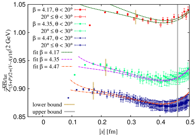
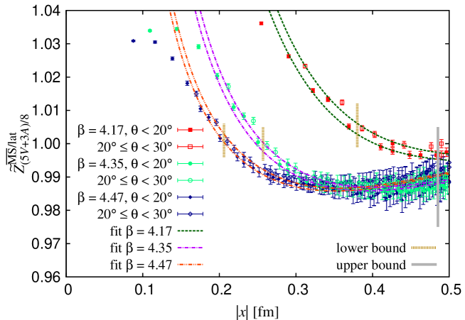
Figure 19: Z~(5V+3A)/8MS¯/lat(a;x)superscriptsubscript~𝑍5𝑉3𝐴8¯MSlat𝑎𝑥\widetilde{Z}_{(5V+3A)/8}^{\rm\overline{MS}/lat}(a;x) at the three of β𝛽\beta with Mπ300similar-tosubscript𝑀𝜋300M_{\pi}\sim 300 MeV. For each β𝛽\beta, the results at smaller ams𝑎subscript𝑚𝑠am_{s} is plotted. The data at θ<20𝜃superscript20\theta<20^{\circ} (filled points) and 20θ<30superscript20𝜃superscript3020^{\circ}\leq\theta<30^{\circ} (open points) are separately plotted. The fit results for both θ<20𝜃superscript20\theta<20^{\circ} and 20θ<30superscript20𝜃superscript3020^{\circ}\leq\theta<30^{\circ} are also plotted by the curves.

Figure 19 shows Z~(5V+3A)/8MS¯/lat(a;x)superscriptsubscript~𝑍5𝑉3𝐴8¯MSlat𝑎𝑥\widetilde{Z}_{(5V+3A)/8}^{\rm\overline{MS}/lat}(a;x) obtained at three β𝛽\beta values with approximately matched quark masses. The position where Z~(5V+3A)/8MS¯/lat(a;x)superscriptsubscript~𝑍5𝑉3𝐴8¯MSlat𝑎𝑥\widetilde{Z}_{(5V+3A)/8}^{\rm\overline{MS}/lat}(a;x) starts deviating from a constant toward short distances moves as the lattice spacing is reduced, indicating that this deviation is due to the discretization effects. The most significant discretization effect is of O(a2)𝑂superscript𝑎2O(a^{2}) which appears as (a/x)2superscript𝑎𝑥2(a/x)^{2}. Since we already subtract discretization effects at the tree-level, αs(β)(a/x)2subscript𝛼𝑠𝛽superscript𝑎𝑥2\alpha_{s}(\beta)(a/x)^{2} is the leading remaining discretization effects. As discussed in Section IV.2, we discard the data in θ30𝜃superscript30\theta\geq 30^{\circ} and parametrize the discretization effects in 0θ<20superscript0𝜃superscript200^{\circ}\leq\theta<20^{\circ} and in 20θ<30superscript20𝜃superscript3020^{\circ}\leq\theta<30^{\circ} separately as described below.

We determine ZVMS¯/latsuperscriptsubscript𝑍𝑉¯MSlatZ_{V}^{\rm\overline{MS}/lat} by a simultaneous fit of the data on all ensembles using the fit function

Z~(5V+3A)/8MS¯/lat(a;x)superscriptsubscript~𝑍5𝑉3𝐴8¯MSlat𝑎𝑥\displaystyle\widetilde{Z}_{(5V+3A)/8}^{\rm\overline{MS}/lat}(a;x) =ZVMS¯/lat(β)absentsuperscriptsubscript𝑍𝑉¯MSlat𝛽\displaystyle=Z_{V}^{\rm\overline{MS}/lat}(\beta)
+C2(θ)αs(β)(a/x)2+C4,Gx4+(C6,q+C6,mGmq2+C6,mqmq3)x6,subscript𝐶2𝜃subscript𝛼𝑠𝛽superscript𝑎𝑥2subscript𝐶4𝐺superscript𝑥4subscript𝐶6𝑞subscript𝐶6𝑚𝐺superscriptsubscript𝑚𝑞2subscript𝐶6𝑚𝑞superscriptsubscript𝑚𝑞3superscript𝑥6\displaystyle+C_{-2}(\theta)\alpha_{s}(\beta)(a/x)^{2}+C_{4,G}x^{4}+(C_{6,q}+C_{6,mG}m_{q}^{2}+C_{6,mq}m_{q}^{3})x^{6}, (31)

with nine free parameters ZVMS¯/lat(4.17)superscriptsubscript𝑍𝑉¯MSlat4.17Z_{V}^{\rm\overline{MS}/lat}(4.17), ZVMS¯/lat(4.35)superscriptsubscript𝑍𝑉¯MSlat4.35Z_{V}^{\rm\overline{MS}/lat}(4.35), ZVMS¯/lat(4.47)superscriptsubscript𝑍𝑉¯MSlat4.47Z_{V}^{\rm\overline{MS}/lat}(4.47), C2(θ<20)subscript𝐶2𝜃superscript20C_{-2}(\theta<20^{\circ}), C2(20θ<30)subscript𝐶2superscript20𝜃superscript30C_{-2}(20^{\circ}\leq\theta<30^{\circ}), C4,Gsubscript𝐶4𝐺C_{4,G} , C6,qsubscript𝐶6𝑞C_{6,q}, C6,mGsubscript𝐶6𝑚𝐺C_{6,mG}, and C6,mqsubscript𝐶6𝑚𝑞C_{6,mq}. Here, the last four parameters correspond to the contribution of asGGdelimited-⟨⟩subscript𝑎𝑠𝐺𝐺\langle a_{s}GG\rangle, q¯qq¯qdelimited-⟨⟩¯𝑞𝑞¯𝑞𝑞\langle\bar{q}q\bar{q}q\rangle, mq2GGsuperscriptsubscript𝑚𝑞2delimited-⟨⟩𝐺𝐺m_{q}^{2}\langle GG\rangle, and mq3q¯qsuperscriptsubscript𝑚𝑞3delimited-⟨⟩¯𝑞𝑞m_{q}^{3}\langle\bar{q}q\rangle, respectively. In this analysis, we neglect the O(as)𝑂subscript𝑎𝑠O(a_{s}) correction to the Wilson coefficients of these operators. The terms of O(x6)𝑂superscript𝑥6O(x^{6}) involve the logarithmic dependence ln(x/x0)2\ln(x/x_{0})^{2} as discussed in Section III.2. Here we do not consider this effect because ln(x/x0)2\ln(x/x_{0})^{2} is roughly constant in the fit range and their effects cannot be identified. The fit results are shown in Fig. 19 by the curves. Here, both the results for θ<20𝜃superscript20\theta<20^{\circ} and 20θ<30superscript20𝜃superscript3020^{\circ}\leq\theta<30^{\circ} are plotted.

Table 2: Result for the renormalization factor ZVMS¯/lat(a)superscriptsubscript𝑍𝑉¯MSlat𝑎Z_{V}^{\rm\overline{MS}/lat}(a) of the vector channel.
β𝛽\beta ZVMS¯/lat(a)superscriptsubscript𝑍𝑉¯MSlat𝑎\ Z_{V}^{\rm\overline{MS}/lat}(a) Errors
Stat. Disc. μxsubscriptsuperscript𝜇𝑥\mu^{*}_{x} ΛQCDsubscriptΛQCD\Lambda_{\rm QCD}
 4.17  0.9553 (53) (74) (8) (5)
 4.35  0.9636 (34) (46) (7) (4)
 4.47  0.9699 (26) (38) (6) (4)

In Table 2, the results for ZVMS¯/latsuperscriptsubscript𝑍𝑉¯MSlatZ_{V}^{\rm\overline{MS}/lat} are summarized with the errors from various sources. The first error is the statistical error. The second represents the discretization error. The central value is the fit result with a lower bound (xlow/a)2=23superscriptsubscript𝑥low𝑎223(x_{\rm low}/a)^{2}=23, which is shown in Fig. 19. and the second error is estimated by moving the lower bound in the region 19(xlow/a)22719superscriptsubscript𝑥low𝑎22719\leq(x_{\rm low}/a)^{2}\leq 27 and taking the largest difference from the central value. The third is an estimate of the uncertainty of the higher order corrections of the perturbative expansion as discussed in Section III.1. The central value is calculated with μx,optsuperscriptsubscript𝜇𝑥opt\mu_{x}^{*,\rm opt} in (10) and the uncertainty is estimated by the maximum difference of results with μxsubscriptsuperscript𝜇𝑥\mu^{*}_{x} in the region [12μx,opt,2μx,opt]12superscriptsubscript𝜇𝑥opt2superscriptsubscript𝜇𝑥opt[{1\over 2}\mu_{x}^{*,\rm opt},2\mu_{x}^{*,\rm opt}]. The last error is from the uncertainty of ΛQCDsubscriptΛQCD\Lambda_{\rm QCD} or of the strong coupling constant. We use the value ΛQCDMS¯,nf=3=340(8)superscriptsubscriptΛQCD¯MSsubscript𝑛𝑓33408\Lambda_{\rm QCD}^{{\rm\overline{MS}},n_{f}=3}=340(8) MeV reported by Particle Data Group Agashe:2014kda . The uncertainty of the lattice spacing does not significantly affect the results. The upper bound of the fit range is fixed to 0.485 fm.

The fit result for other parameters reads

C2(θ<20)=14.0(1.2)(2.0)(1)(1),C2(20θ<30)=15.1(1.1)(2.2)(1)(),C4,G=0.564(190)(187)(99)(14)fm4,C6,q=0.109(61)(56)(4)(3)fm6,C6,mG=19.8(31.5)(5)(3)(1)fm4,C6,mq=192(125)(2)(2)(1)fm3.subscript𝐶2𝜃superscript2014.01.22.011subscript𝐶2superscript20𝜃superscript3015.11.12.21subscript𝐶4𝐺0.5641901879914superscriptfm4subscript𝐶6𝑞0.109615643superscriptfm6subscript𝐶6𝑚𝐺19.831.5531superscriptfm4subscript𝐶6𝑚𝑞192125221superscriptfm3\begin{array}[]{ll}C_{-2}(\theta<20^{\circ})=14.0(1.2)(2.0)(1)(1),&C_{-2}(20^{\circ}\leq\theta<30^{\circ})=15.1(1.1)(2.2)(1)(\--),\\ C_{4,G}=0.564(190)(187)(99)(14)\rm\ fm^{-4},&C_{6,q}=-0.109(61)(56)(4)(3)\rm\ fm^{-6},\\ C_{6,mG}=-19.8(31.5)(5)(3)(1)\rm\ fm^{-4},&C_{6,mq}=192(125)(2)(2)(1)\rm\ fm^{-3}.\end{array}

The consistency of this analysis can be checked by evaluating the gluon condensate from the fit result. Using (20) and the fit result C4,Gsubscript𝐶4𝐺C_{4,G}, we obtain (αs/π)GG=0.017(6)(6)(3)delimited-⟨⟩subscript𝛼𝑠𝜋𝐺𝐺0.017663\langle(\alpha_{s}/\pi)GG\rangle=0.017(6)(6)(3) ()GeV4superscriptGeV4(\--)\rm\ GeV^{4} at the lowest order of αs/πsubscript𝛼𝑠𝜋\alpha_{s}/\pi. The errors are estimated in the similar manner. This result is in good agreement with known values, e.g. (αs/π)GG=0.012GeV4delimited-⟨⟩subscript𝛼𝑠𝜋𝐺𝐺0.012superscriptGeV4\langle(\alpha_{s}/\pi)GG\rangle=0.012\rm\ GeV^{4} from the sum rule for charmonium Shifman:1978bx and (αs/π)GG=0.006(12)GeV4delimited-⟨⟩subscript𝛼𝑠𝜋𝐺𝐺0.00612superscriptGeV4\langle(\alpha_{s}/\pi)GG\rangle=0.006(12)\rm\ GeV^{4} from the spectral functions of hadronic τ𝜏\tau decays Geshkenbein:2001mn .

V.2 Determination of ZSsubscript𝑍𝑆Z_{S}

The domain-wall fermion also guarantees the agreement of the renormalization constants of the scalar ZSMS¯/lat(a)superscriptsubscript𝑍𝑆¯MSlat𝑎Z_{S}^{\rm\overline{MS}/lat}(a) and pseudoscalar ZPMS¯/lat(a)superscriptsubscript𝑍𝑃¯MSlat𝑎Z_{P}^{\rm\overline{MS}/lat}(a) densities. The determination of ZSMS¯/lat(a)superscriptsubscript𝑍𝑆¯MSlat𝑎Z_{S}^{\rm\overline{MS}/lat}(a) and ZPMS¯/lat(a)superscriptsubscript𝑍𝑃¯MSlat𝑎Z_{P}^{\rm\overline{MS}/lat}(a) may be more complicated due to the instanton-induced ’t Hooft interactions 'tHooft:1976fv ; Novikov:1981xi , which affect the scalar and pseudoscalar correlators significantly and are not described by OPE. Since the instanton effects to the scalar and pseudoscalar correlators are the same magnitude with an opposite sign, the naïve average 12(ΠS(x)+ΠP(x))12subscriptΠ𝑆𝑥subscriptΠ𝑃𝑥{1\over 2}(\Pi_{S}(x)+\Pi_{P}(x)) may cancel such effects and could be well explained by OPE. The average contains the contribution of the chiral condensate in OPE, which we try to cancel by using the difference between the vector and axial-vector correlators. Namely, we analyze

Z~(S+P)/2+(VA)/16MS¯/latsuperscriptsubscript~𝑍𝑆𝑃2𝑉𝐴16¯MSlat\displaystyle\widetilde{Z}_{(S+P)/2+(V-A)/16}^{\rm\overline{MS}/lat} (2GeV,a;x)2GeV𝑎𝑥\displaystyle({\rm 2\ GeV},a;x)
=\displaystyle= ΠSMS¯(2GeV;x)12(ΠSlat(a;x)+ΠPlat(a;x))+116(ΠVlat(a;x)ΠAlat(a;x)),superscriptsubscriptΠ𝑆¯MS2GeV𝑥12superscriptsubscriptΠ𝑆lat𝑎𝑥superscriptsubscriptΠ𝑃lat𝑎𝑥116superscriptsubscriptΠ𝑉lat𝑎𝑥superscriptsubscriptΠ𝐴lat𝑎𝑥\displaystyle\sqrt{\Pi_{S}^{\rm\overline{MS}}({\rm 2\ GeV};x)\over{1\over 2}\big{(}\Pi_{S}^{\rm lat}(a;x)+\Pi_{P}^{\rm lat}(a;x)\big{)}+{1\over 16}\big{(}\Pi_{V}^{\rm lat}(a;x)-\Pi_{A}^{\rm lat}(a;x)\big{)}}, (32)

whose OPE does not depend on the chiral condensate mqq¯qx4subscript𝑚𝑞delimited-⟨⟩¯𝑞𝑞superscript𝑥4m_{q}\langle\bar{q}q\rangle x^{4} at the tree-level. Since we neglect the O(as)𝑂subscript𝑎𝑠O(a_{s}) correction to the Wilson coefficients in this analysis, we omit the renormalization factor for ΠVlat(a;x)ΠAlat(a;x)superscriptsubscriptΠ𝑉lat𝑎𝑥superscriptsubscriptΠ𝐴lat𝑎𝑥\Pi_{V}^{\rm lat}(a;x)-\Pi_{A}^{\rm lat}(a;x).

Refer to caption
Figure 20: Same as Fig. 19 but for Z~(S+P)/2+(VA)/16MS¯(2GeV,a;x)superscriptsubscript~𝑍𝑆𝑃2𝑉𝐴16¯MS2GeV𝑎𝑥\widetilde{Z}_{(S+P)/2+(V-A)/16}^{\rm\overline{MS}}({\rm 2\ GeV},a;x)
Table 3: Result for the renormalization factor ZSMS¯/lat(2GeV,a)superscriptsubscript𝑍𝑆¯MSlat2GeV𝑎Z_{S}^{\rm\overline{MS}/lat}({2\rm\ GeV},a) of the scalor channel.
β𝛽\beta ZSMS¯/lat(2GeV,a)superscriptsubscript𝑍𝑆¯MSlat2GeV𝑎\ Z_{S}^{\rm\overline{MS}/lat}({2\rm\ GeV},a) Errors
Stat. Disc. μxsuperscriptsubscript𝜇𝑥\mu_{x}^{*} ΛQCDsubscriptΛQCD\Lambda_{\rm QCD}
 4.17  1.0372 (93) (77) (57) (58)
 4.35  0.9342 (57) (43) (37) (34)
 4.47  0.8926 (41) (35) (30) (25)

We implement the simultaneous fit to the data of (32) with the same function as (31). The results are summarized in Table 3. The error estimation is done in the similar manner as that for the vector channel. We choose the lower bound of the fit range as (xlow/a)2=16superscriptsubscript𝑥low𝑎216(x_{\rm low}/a)^{2}=16 for the central value and estimate the second error by changing xlowsubscript𝑥lowx_{\rm low} in the region 12(xlow/a)22012superscriptsubscript𝑥low𝑎22012\leq(x_{\rm low}/a)^{2}\leq 20. The central μx=μx,optsuperscriptsubscript𝜇𝑥superscriptsubscript𝜇𝑥opt\mu_{x}^{*}=\mu_{x}^{*,\rm opt} is given by (14) and the third error is estimated by varying μxsuperscriptsubscript𝜇𝑥\mu_{x}^{*} in the region [11.6μx,opt,1.6μx,opt]11.6superscriptsubscript𝜇𝑥opt1.6superscriptsubscript𝜇𝑥opt[{1\over 1.6}\mu_{x}^{*,\rm opt},1.6\mu_{x}^{*,\rm opt}]. The upper bound of the fit range is fixed to 0.460 fm. The fit result is shown in Fig. 20 for the same ensembles as in Fig. 19.

The fit result for other parameters reads

C2(θ<20)=2.25(1.37)(1.81)(58)(77),C2(20θ<30)=0.522(1.39)(1.72)(60)(80),C4,G=2.27(52)(25)(23)(33)fm4,C6,q=7.71(52)(1.08)(2.19)(45)fm6,C6,mG=212(156)(4)(3)(2)fm4,C6,mq=432(622)(18)(7)(3)fm3.subscript𝐶2𝜃superscript202.251.371.815877subscript𝐶2superscript20𝜃superscript300.5221.391.726080subscript𝐶4𝐺2.2752252333superscriptfm4subscript𝐶6𝑞7.71521.082.1945superscriptfm6subscript𝐶6𝑚𝐺212156432superscriptfm4subscript𝐶6𝑚𝑞4326221873superscriptfm3\begin{array}[]{ll}C_{-2}(\theta<20^{\circ})=2.25(1.37)(1.81)(58)(77),&C_{-2}(20^{\circ}\leq\theta<30^{\circ})=0.522(1.39)(1.72)(60)(80),\\ C_{4,G}=-2.27(52)(25)(23)(33)\rm\ fm^{-4},&C_{6,q}=7.71(52)(1.08)(2.19)(45)\rm\ fm^{-6},\\ C_{6,mG}=212(156)(4)(3)(2)\rm\ fm^{-4},&C_{6,mq}=-432(622)(18)(7)(3)\rm\ fm^{-3}.\end{array}

VI Conclusion

We have determined the renormalization factors ZVMS¯/lat(a)superscriptsubscript𝑍𝑉¯MSlat𝑎Z_{V}^{\rm\overline{MS}/lat}(a), ZSMS¯/lat(2GeV,a)superscriptsubscript𝑍𝑆¯MSlat2GeV𝑎Z_{S}^{\rm\overline{MS}/lat}({2\rm\ GeV},a) of the flavor non-singlet quark bilinear operators composed of Möbius domain-wall fermions by analyzing correlation functions in the coordinate space. This method enables us to renormalize in a fully gauge invariant manner and to implement the perturbative matching up to the four-loop level. We impose the direct renormalization condition onto the MS¯¯MS\rm\overline{MS} scheme without introducing any intermediate renormalization schemes.

Although the complicated analysis is required to eliminate discretization effects that are significant at short distances, the results obtained in this work and their accuracy demonstrate the use of the X-space method. It is already at a competing level with the RI/MOM methods, and we expect it becomes more so in the future as the lattice spacing is reduced, because the perturbative error would become the dominant source in such situation.

Direct applications of our results are the calculation of meson decay constants and quark masses. Some preliminary results are found in Fahy:2015xka . The (pseudo)scalar renormalization factor is also necessary for the determination of the chiral condensate, which characterizes the spontaneous broken chiral symmetry in QCD. We can extract this important quantity from the same set of correlators as we analyzed in this work, through the axial Ward-Takahashi identity. Such analysis will be presented in a forthcoming paper. The same quantity can be obtained with a completely different method, i.e. from the eigenvalue density of the Dirac operator through the Banks-Casher relation. A preliminary analysis on our ensembles was presented in Cossu:2016yzp .

Current correlators at short distances contain more information of QCD. They are complicated mixture of excited states of hadrons, but at the same time they can be analyzed using perturbation theory. For the analysis of the intermediate region between perturbative and non-perturbative regimes, the lattice data may provide useful information, that can be used to study the range of application of perturbative expansion in perturbative QCD for instance. The work in such directions are in progress.

Acknowledgements.
Numerical simulations are performed on Hitachi SR 16000 and IBM System Blue Gene Solution at KEK under a support of its Large Scale Simulation Program (No. 13/14-04, 14/15-10). We thank P. Boyle for the optimized code for BGQ. This work is supported in part by the Grant-in-Aid of the Japanese Ministry of Education (No. 25800147, 26247043, 26400259,15K05065) and by MEXT SPIRE and JICFuS.

Appendix A Summary of perturbative coefficients

This appendix summarizes numerical coefficients of perturbative expansions of the vector and scalar correlators obtained by using the four-loop results of correlators Chetyrkin:2010dx , the beta function vanRitbergen:1997va , and the anomalous dimension Chetyrkin:1997dh ; Vermaseren:1997fq .

For the vector channel, the perturbative coefficients CiVsuperscriptsubscript𝐶𝑖𝑉C_{i}^{V}’s at μx=μxsuperscriptsubscript𝜇𝑥subscript𝜇𝑥\mu_{x}^{*}=\mu_{x} and the corresponding perturbative expansion with nf=3subscript𝑛𝑓3n_{f}=3 are

C1V(μx)=1,superscriptsubscript𝐶1𝑉subscript𝜇𝑥1\displaystyle C_{1}^{V}(\mu_{x})=1,
C2V(μx)=5.5269+0.34002nf,superscriptsubscript𝐶2𝑉subscript𝜇𝑥5.52690.34002subscript𝑛𝑓\displaystyle C_{2}^{V}(\mu_{x})=-5.5269+0.34002n_{f},
C3V(μx)=10.4153.2912nf+0.12602nf2,superscriptsubscript𝐶3𝑉subscript𝜇𝑥10.4153.2912subscript𝑛𝑓0.12602superscriptsubscript𝑛𝑓2\displaystyle C_{3}^{V}(\mu_{x})=10.415-3.2912n_{f}+0.12602n_{f}^{2},
C4V(μx)=28.928+30.966nf2.6652nf2+0.064007nf3,superscriptsubscript𝐶4𝑉subscript𝜇𝑥28.92830.966subscript𝑛𝑓2.6652superscriptsubscript𝑛𝑓20.064007superscriptsubscript𝑛𝑓3\displaystyle C_{4}^{V}(\mu_{x})=28.928+30.966n_{f}-2.6652n_{f}^{2}+0.064007n_{f}^{3}, (33)
ΠVMS¯(x)|nf=3=6π4x6(1\displaystyle\Pi_{V}^{\rm\overline{MS}}(x)\Big{|}_{n_{f}=3}={6\over\pi^{4}x^{6}}\Big{(}1 +as(μx)4.5069as(μx)2subscript𝑎𝑠subscript𝜇𝑥4.5069subscript𝑎𝑠superscriptsubscript𝜇𝑥2\displaystyle+a_{s}(\mu_{x})-4.5069a_{s}(\mu_{x})^{2}
+1.6758as(μx)3+99.567as(μx)4+O(as5)).\displaystyle+1.6758a_{s}(\mu_{x})^{3}+99.567a_{s}(\mu_{x})^{4}+O(a_{s}^{5})\Big{)}. (34)

At μx=μ~xsuperscriptsubscript𝜇𝑥subscript~𝜇𝑥\mu_{x}^{*}=\tilde{\mu}_{x}, CiVsubscriptsuperscript𝐶𝑉𝑖C^{V}_{i}’s and the expansion are given by

C1V(μ~x)=1,superscriptsubscript𝐶1𝑉subscript~𝜇𝑥1\displaystyle C_{1}^{V}(\tilde{\mu}_{x})=1,
C2V(μ~x)=4.8893+0.30137nf,superscriptsubscript𝐶2𝑉subscript~𝜇𝑥4.88930.30137subscript𝑛𝑓\displaystyle C_{2}^{V}(\tilde{\mu}_{x})=-4.8893+0.30137n_{f},
C3V(μ~x)=5.25172.6633nf+0.10124nf2,superscriptsubscript𝐶3𝑉subscript~𝜇𝑥5.25172.6633subscript𝑛𝑓0.10124superscriptsubscript𝑛𝑓2\displaystyle C_{3}^{V}(\tilde{\mu}_{x})=5.2517-2.6633n_{f}+0.10124n_{f}^{2},
C4V(μ~x)=33.562+26.233nf2.2001nf2+0.050863nf3,superscriptsubscript𝐶4𝑉subscript~𝜇𝑥33.56226.233subscript𝑛𝑓2.2001superscriptsubscript𝑛𝑓20.050863superscriptsubscript𝑛𝑓3\displaystyle C_{4}^{V}(\tilde{\mu}_{x})=33.562+26.233n_{f}-2.2001n_{f}^{2}+0.050863n_{f}^{3}, (35)
ΠVMS¯(x)|nf=3=6π4x6(1+\displaystyle\Pi_{V}^{\rm\overline{MS}}(x)\Big{|}_{n_{f}=3}={6\over\pi^{4}x^{6}}\Big{(}1+ as(μ~x)3.9852as(μ~x)2subscript𝑎𝑠subscript~𝜇𝑥3.9852subscript𝑎𝑠superscriptsubscript~𝜇𝑥2\displaystyle a_{s}(\tilde{\mu}_{x})-3.9852a_{s}(\tilde{\mu}_{x})^{2}
\displaystyle- 1.8270as(μ~x)3+93.835as(μ~x)4+O(as5)).\displaystyle 1.8270a_{s}(\tilde{\mu}_{x})^{3}+93.835a_{s}(\tilde{\mu}_{x})^{4}+O(a_{s}^{5})\Big{)}. (36)

Finally, at μx=μ~xsuperscriptsubscript𝜇𝑥subscript~𝜇𝑥\mu_{x}^{*}=\tilde{\mu}_{x}, CiVsubscriptsuperscript𝐶𝑉𝑖C^{V}_{i}’s and the expansion are

C1V(μxBLM)=1,superscriptsubscript𝐶1𝑉superscriptsubscript𝜇𝑥BLM1\displaystyle C_{1}^{V}(\mu_{x}^{\rm BLM})=1,
C2V(μxBLM)=0.083333,superscriptsubscript𝐶2𝑉superscriptsubscript𝜇𝑥BLM0.083333\displaystyle C_{2}^{V}(\mu_{x}^{\rm BLM})=0.083333,
C3V(μxBLM)=7.11911.1478nf+0.010414nf2,superscriptsubscript𝐶3𝑉superscriptsubscript𝜇𝑥BLM7.11911.1478subscript𝑛𝑓0.010414superscriptsubscript𝑛𝑓2\displaystyle C_{3}^{V}(\mu_{x}^{\rm BLM})=-7.1191-1.1478n_{f}+0.010414n_{f}^{2},
C4V(μxBLM)=56.886+12.283nf0.58326nf2+0.014075nf3,superscriptsubscript𝐶4𝑉superscriptsubscript𝜇𝑥BLM56.88612.283subscript𝑛𝑓0.58326superscriptsubscript𝑛𝑓20.014075superscriptsubscript𝑛𝑓3\displaystyle C_{4}^{V}(\mu_{x}^{\rm BLM})=-56.886+12.283n_{f}-0.58326n_{f}^{2}+0.014075n_{f}^{3}, (37)
ΠVMS¯(x)|nf=3=6π4x6(1+\displaystyle\Pi_{V}^{\rm\overline{MS}}(x)\Big{|}_{n_{f}=3}={6\over\pi^{4}x^{6}}\Big{(}1+ as(μxBLM)+0.083333as(μxBLM)2subscript𝑎𝑠superscriptsubscript𝜇𝑥BLM0.083333subscript𝑎𝑠superscriptsuperscriptsubscript𝜇𝑥BLM2\displaystyle a_{s}(\mu_{x}^{\rm BLM})+0.083333a_{s}(\mu_{x}^{\rm BLM})^{2}
\displaystyle- 10.469as(μxBLM)324.907as(μxBLM)4+O(as5)).\displaystyle 10.469a_{s}(\mu_{x}^{\rm BLM})^{3}-24.907a_{s}(\mu_{x}^{\rm BLM})^{4}+O(a_{s}^{5})\Big{)}. (38)

For the scalar channel, the perturbative coefficients CiSsuperscriptsubscript𝐶𝑖𝑆C_{i}^{S}’s at μx=μx=μxsuperscriptsubscript𝜇𝑥superscriptsubscript𝜇𝑥subscript𝜇𝑥\mu_{x}^{*}=\mu_{x}^{\prime}=\mu_{x} and the corresponding expansion with nf=3subscript𝑛𝑓3n_{f}=3 are

C1S(μx,μx)=0.20294,superscriptsubscript𝐶1𝑆subscript𝜇𝑥subscript𝜇𝑥0.20294\displaystyle C_{1}^{S}(\mu_{x},\mu_{x})=0.20294,
C2S(μx,μx)=20.197+0.56314nf,superscriptsubscript𝐶2𝑆subscript𝜇𝑥subscript𝜇𝑥20.1970.56314subscript𝑛𝑓\displaystyle C_{2}^{S}(\mu_{x},\mu_{x})=-20.197+0.56314n_{f},
C3S(μx,μx)=7.88547.5318nf+0.37635nf2,superscriptsubscript𝐶3𝑆subscript𝜇𝑥subscript𝜇𝑥7.88547.5318subscript𝑛𝑓0.37635superscriptsubscript𝑛𝑓2\displaystyle C_{3}^{S}(\mu_{x},\mu_{x})=7.8854-7.5318n_{f}+0.37635n_{f}^{2},
C4S(μx,μx)=500.95+40.402nf5.3403nf2+0.18479nf3,superscriptsubscript𝐶4𝑆subscript𝜇𝑥subscript𝜇𝑥500.9540.402subscript𝑛𝑓5.3403superscriptsubscript𝑛𝑓20.18479superscriptsubscript𝑛𝑓3\displaystyle C_{4}^{S}(\mu_{x},\mu_{x})=500.95+40.402n_{f}-5.3403n_{f}^{2}+0.18479n_{f}^{3}, (39)
ΠSMS¯(μx;x)|nf=3=3π4x6(1\displaystyle\Pi_{S}^{\rm\overline{MS}}(\mu_{x};x)\Big{|}_{n_{f}=3}={3\over\pi^{4}x^{6}}\Big{(}1 +0.20294as(μx)18.507as(μx)20.20294subscript𝑎𝑠subscript𝜇𝑥18.507subscript𝑎𝑠superscriptsubscript𝜇𝑥2\displaystyle+0.20294a_{s}(\mu_{x})-18.507a_{s}(\mu_{x})^{2}
11.323as(μx)3+579.08as(μx)4+O(as5)).\displaystyle-11.323a_{s}(\mu_{x})^{3}+579.08a_{s}(\mu_{x})^{4}+O(a_{s}^{5})\Big{)}. (40)

At μx=μx=μ~xsuperscriptsubscript𝜇𝑥superscriptsubscript𝜇𝑥subscript~𝜇𝑥\mu_{x}^{*}=\mu_{x}^{\prime}=\tilde{\mu}_{x}, CiSsuperscriptsubscript𝐶𝑖𝑆C_{i}^{S}’s and the expansion are given by

C1S(μ~x,μ~x)=23,superscriptsubscript𝐶1𝑆subscript~𝜇𝑥subscript~𝜇𝑥23\displaystyle C_{1}^{S}(\tilde{\mu}_{x},\tilde{\mu}_{x})={2\over 3},
C2S(μ~x,μ~x)=17.766+0.48193nf,superscriptsubscript𝐶2𝑆subscript~𝜇𝑥subscript~𝜇𝑥17.7660.48193subscript𝑛𝑓\displaystyle C_{2}^{S}(\tilde{\mu}_{x},\tilde{\mu}_{x})=-17.766+0.48193n_{f},
C3S(μ~x,μ~x)=14.6566.3172nf+0.32333nf2,superscriptsubscript𝐶3𝑆subscript~𝜇𝑥subscript~𝜇𝑥14.6566.3172subscript𝑛𝑓0.32333superscriptsubscript𝑛𝑓2\displaystyle C_{3}^{S}(\tilde{\mu}_{x},\tilde{\mu}_{x})=-14.656-6.3172n_{f}+0.32333n_{f}^{2},
C4S(μ~x,μ~x)=450.45+25.502nf3.8057nf2+0.14697nf3,superscriptsubscript𝐶4𝑆subscript~𝜇𝑥subscript~𝜇𝑥450.4525.502subscript𝑛𝑓3.8057superscriptsubscript𝑛𝑓20.14697superscriptsubscript𝑛𝑓3\displaystyle C_{4}^{S}(\tilde{\mu}_{x},\tilde{\mu}_{x})=450.45+25.502n_{f}-3.8057n_{f}^{2}+0.14697n_{f}^{3}, (41)
ΠSMS¯(μ~x;x)|nf=3=3π4x6(1\displaystyle\Pi_{S}^{\rm\overline{MS}}(\tilde{\mu}_{x};x)\Big{|}_{n_{f}=3}={3\over\pi^{4}x^{6}}\Big{(}1 +0.66667as(μ~x)16.321as(μ~x)20.66667subscript𝑎𝑠subscript~𝜇𝑥16.321subscript𝑎𝑠superscriptsubscript~𝜇𝑥2\displaystyle+0.66667a_{s}(\tilde{\mu}_{x})-16.321a_{s}(\tilde{\mu}_{x})^{2}
30.698as(μ~x)3+496.67as(μ~x)4+O(as5)).\displaystyle-30.698a_{s}(\tilde{\mu}_{x})^{3}+496.67a_{s}(\tilde{\mu}_{x})^{4}+O(a_{s}^{5})\Big{)}. (42)

Appendix B Mean field approximation of correlators on the lattice

Correlators in the coordinate space are given by

ΠΓ(x)=Tr[SF(x)ΓSF(x)Γ],subscriptΠΓ𝑥delimited-⟨⟩Trdelimited-[]subscript𝑆𝐹𝑥Γsubscript𝑆𝐹𝑥Γ\Pi_{\Gamma}(x)=\left\langle{\rm{Tr}}\big{[}S_{F}(x)\Gamma S_{F}(-x)\Gamma\big{]}\right\rangle, (43)

where SF(x)subscript𝑆𝐹𝑥S_{F}(x) stands for the propagator of the Dirac field. We give the mean field approximation of the domain-wall propagator and its asymptotic form in the long-distance limit. Since the residual mass in this work is almost negligible, we consider the domain-wall propagator with the infinite size of the fifth direction Lssubscript𝐿𝑠L_{s}\rightarrow\infty. The four-dimensional representation S~FDW(q,mq)superscriptsubscript~𝑆𝐹DW𝑞subscript𝑚𝑞\widetilde{S}_{F}^{\rm DW}(q,m_{q}) of the mean field domain-wall propagator in the momentum space is Narayanan:1992wx ; Shamir:1993zy ; Aoki:1997xg

S~FDW(q,mq)/a=iγμu0sin(aqμ)+(1Weα)amq1+Weα+(1Weα)(amq)2,superscriptsubscript~𝑆𝐹DW𝑞subscript𝑚𝑞𝑎isubscript𝛾𝜇subscript𝑢0𝑎subscript𝑞𝜇1𝑊superscripte𝛼𝑎subscript𝑚𝑞1𝑊superscripte𝛼1𝑊superscripte𝛼superscript𝑎subscript𝑚𝑞2\widetilde{S}_{F}^{\rm DW}(q,m_{q})/a={-{\rm{i}}\gamma_{\mu}u_{0}\sin(aq_{\mu})+(1-W{\rm{e}}^{-\alpha})am_{q}\over-1+W{\rm{e}}^{\alpha}+(1-W{\rm{e}}^{-\alpha})(am_{q})^{2}}, (44)

where W𝑊W and α𝛼\alpha are defined by

W(q)𝑊𝑞\displaystyle W(q) =1M0+μ(1u0cos(aqμ)),absent1subscript𝑀0subscript𝜇1subscript𝑢0𝑎subscript𝑞𝜇\displaystyle=1-M_{0}+\sum_{\mu}\big{(}1-u_{0}\cos(aq_{\mu})\big{)}, (45)
coshα(q)𝛼𝑞\displaystyle\cosh\alpha(q) =1+W2+u02μsin2(aqμ)2W,absent1superscript𝑊2superscriptsubscript𝑢02subscript𝜇superscript2𝑎subscript𝑞𝜇2𝑊\displaystyle={1+W^{2}+u_{0}^{2}\sum_{\mu}\sin^{2}(aq_{\mu})\over 2W}, (46)

with M0subscript𝑀0M_{0} and u0subscript𝑢0u_{0} being the domain-wall mass parameter and the fourth root of the plaquette expectation value, respectively. The free propagator is reproduced by putting u0=1subscript𝑢01u_{0}=1.

The propagator in the coordinate space is calculated by a numerical Fourier transform in a finite box L4superscript𝐿4L^{4},

SFDW,L4(x,mq)=1L4qS~FDW(q)eiqx,superscriptsubscript𝑆𝐹DWsuperscript𝐿4𝑥subscript𝑚𝑞1superscript𝐿4subscript𝑞superscriptsubscript~𝑆𝐹DW𝑞superscriptei𝑞𝑥S_{F}^{{\rm DW},L^{4}}(x,m_{q})={1\over L^{4}}\sum_{q}\widetilde{S}_{F}^{\rm DW}(q){\rm{e}}^{{\rm{i}}qx}, (47)

where the sum over q𝑞q for the periodic boundary condition runs over

q{2πL(k1,k2,k3,k4)|kμ=L2a+1,L2a+2,,L2a},𝑞conditional-set2𝜋𝐿subscript𝑘1subscript𝑘2subscript𝑘3subscript𝑘4subscript𝑘𝜇𝐿2𝑎1𝐿2𝑎2𝐿2𝑎q\in\left\{{2\pi\over L}(k_{1},k_{2},k_{3},k_{4})\ \Big{|}\ k_{\mu}=-{L\over 2a}+1,-{L\over 2a}+2,\cdots,{L\over 2a}\right\}, (48)

The mean field approximation of the propagator of a light quark in a finite box (mqL1)less-than-or-similar-tosubscript𝑚𝑞𝐿1(m_{q}L\lesssim 1) involves large finite volume effects because quarks are in the deconfining phase. Since the numerical Fourier transform in sufficient large volumes is expensive, we apply a correction for the domain-wall propagator as we applied for the propagators of bosonic fields in Section IV.3,

SFDW,(x,mq)superscriptsubscript𝑆𝐹DW𝑥subscript𝑚𝑞\displaystyle S_{F}^{\rm DW,\infty}(x,m_{q}) =SFDW,L4(x,mq)x0SFDW,(xx0,mq)absentsuperscriptsubscript𝑆𝐹DWsuperscript𝐿4𝑥subscript𝑚𝑞subscriptsubscript𝑥0superscriptsubscript𝑆𝐹DW𝑥subscript𝑥0subscript𝑚𝑞\displaystyle=S_{F}^{{\rm DW},L^{4}}(x,m_{q})-\sum_{x_{0}}S_{F}^{\rm DW,\infty}(x-x_{0},m_{q})
SFDW,L4(x,mq)x0SFDW,asym(xx0,mq),similar-to-or-equalsabsentsuperscriptsubscript𝑆𝐹DWsuperscript𝐿4𝑥subscript𝑚𝑞subscriptsubscript𝑥0superscriptsubscript𝑆𝐹DWasym𝑥subscript𝑥0subscript𝑚𝑞\displaystyle\simeq S_{F}^{{\rm DW},L^{4}}(x,m_{q})-\sum_{x_{0}}S_{F}^{\rm DW,asym}(x-x_{0},m_{q}), (49)

where the sum over x0subscript𝑥0x_{0} runs over

x0{(±L,0,0,0),(0,±L,0,0),(0,0,±L,0),(0,0,0,±L),(±L,±L,0,0),},subscript𝑥0plus-or-minus𝐿0000plus-or-minus𝐿0000plus-or-minus𝐿0000plus-or-minus𝐿plus-or-minus𝐿plus-or-minus𝐿00x_{0}\in\{(\pm L,0,0,0),(0,\pm L,0,0),(0,0,\pm L,0),(0,0,0,\pm L),(\pm L,\pm L,0,0),\cdots\}, (50)

and SFDW,asym(x)superscriptsubscript𝑆𝐹DWasym𝑥S_{F}^{\rm DW,asym}(x) is the asymptotic form of the domain-wall propagator in the long-distance limit in the infinite volume, which is calculated as follows.

The domain-wall propagator in the low-momentum region is calculated by expanding (44) at aq0similar-to-or-equals𝑎𝑞0aq\simeq 0,

S~FDW(q,mq)aq0(1δ2)iu0 q /+mqu02q2+mq2+O(δ4),\widetilde{S}_{F}^{\rm DW}(q,m_{q})\xrightarrow{aq\rightarrow 0}(1-\delta^{2}){-{\rm{i}}u_{0}\hbox to0.0pt{\hbox to5.00002pt{\hfil$q$\hfil}\hss}/+m^{\prime}_{q}\over u_{0}^{2}q^{2}+{m^{\prime}_{q}}^{2}}+O(\delta^{4}), (51)

with

δ𝛿\displaystyle\delta =1M0+4(1u0),absent1subscript𝑀041subscript𝑢0\displaystyle=1-M_{0}+4(1-u_{0}), (52)
mqsubscriptsuperscript𝑚𝑞\displaystyle m^{\prime}_{q} =(1δ2)mq.absent1superscript𝛿2subscript𝑚𝑞\displaystyle=(1-\delta^{2})m_{q}. (53)

The Fourier transform of this propagator in the infinite volume gives an asymptotic form in the long-distance limit of the domain-wall propagator,

SFDW,asym(x,mq)=1δ2u04SFcont(x/u0,mq)+O(δ4),superscriptsubscript𝑆𝐹DWasym𝑥subscript𝑚𝑞1superscript𝛿2superscriptsubscript𝑢04superscriptsubscript𝑆𝐹cont𝑥subscript𝑢0subscriptsuperscript𝑚𝑞𝑂superscript𝛿4S_{F}^{\rm DW,asym}(x,m_{q})={1-\delta^{2}\over u_{0}^{4}}S_{F}^{\rm cont}(x/u_{0},m^{\prime}_{q})+O(\delta^{4}), (54)

where the Feynman propagator SFcont(x,mq)superscriptsubscript𝑆𝐹cont𝑥subscript𝑚𝑞S_{F}^{\rm cont}(x,m_{q}) of a Dirac field in the continuum coordinate space is given Zhang:2008jy by

SFcont(x,mq)superscriptsubscript𝑆𝐹cont𝑥subscript𝑚𝑞\displaystyle S_{F}^{\rm cont}(x,m_{q}) =d4q(2π)4eiqxi q /+mqq2+mq2\displaystyle=\int{{\rm{d}}^{4}q\over(2\pi)^{4}}{\rm{e}}^{{\rm{i}}qx}{-{\rm{i}}\hbox to0.0pt{\hbox to5.00002pt{\hfil$q$\hfil}\hss}/+m_{q}\over q^{2}+m_{q}^{2}}
=mq / x4π2|x|3K1(mq|x|)+mq2 / x8π2x2[K0(mq|x|)+K2(mq|x|)]+mq24π2|x|K1(mq|x|),absentsubscript𝑚𝑞 / 𝑥4superscript𝜋2superscript𝑥3subscript𝐾1subscript𝑚𝑞𝑥superscriptsubscript𝑚𝑞2 / 𝑥8superscript𝜋2superscript𝑥2delimited-[]subscript𝐾0subscript𝑚𝑞𝑥subscript𝐾2subscript𝑚𝑞𝑥superscriptsubscript𝑚𝑞24superscript𝜋2𝑥subscript𝐾1subscript𝑚𝑞𝑥\displaystyle={m_{q}\hbox to0.0pt{\hbox to5.71527pt{\hfil/\hfil}\hss}x\over 4\pi^{2}|x|^{3}}K_{1}(m_{q}|x|)+{m_{q}^{2}\hbox to0.0pt{\hbox to5.71527pt{\hfil/\hfil}\hss}x\over 8\pi^{2}x^{2}}\big{[}K_{0}(m_{q}|x|)+K_{2}(m_{q}|x|)\big{]}+{m_{q}^{2}\over 4\pi^{2}|x|}K_{1}(m_{q}|x|), (55)

with Kisubscript𝐾𝑖K_{i} being the modified Bessel functions.

The subtraction by the second line of (49) cannot eliminate discretization effects of wrapping effects, i.e. the subtraction leaves the discretization effects

x0(SFDW,(xx0,mq)SFDW,asym(xx0,mq)),subscriptsubscript𝑥0superscriptsubscript𝑆𝐹DW𝑥subscript𝑥0subscript𝑚𝑞superscriptsubscript𝑆𝐹DWasym𝑥subscript𝑥0subscript𝑚𝑞\sum_{x_{0}}\big{(}S_{F}^{{\rm DW},\infty}(x-x_{0},m_{q})-S_{F}^{\rm DW,asym}(x-x_{0},m_{q})\big{)}, (56)

which are suppressed in large volumes. We observe that these discretization effects are sufficiently small when the calculation is done with mqL1greater-than-or-equivalent-tosubscript𝑚𝑞𝐿1m_{q}L\gtrsim 1.

References