Statistical Hauser-Feshbach theory with width fluctuation correction including direct reaction channels for neutron induced reaction at low energies

Abstract

A model to calculate particle-induced reaction cross sections with statistical Hauser-Feshbach theory including direct reactions is given. The energy average of scattering matrix from the coupled-channels optical model is diagonalized by the transformation proposed by Engelbrecht and Weidenmüller. The ensemble average of $S$-matrix elements in the diagonalized channel space is approximated by a model of Moldauer [Phys.Rev.C 12, 744 (1975)] using newly parametrized channel degree-of-freedom $\nu_{a}$ to better describe the Gaussian Orthogonal Ensemble (GOE) reference calculations. Moldauer approximation is confirmed by a Monte Carlo study using randomly generated $S$-matrix, as well as the GOE three-fold integration formula. The method proposed is applied to the ²³⁸U(n,n’) cross section calculation in the fast energy range, showing an enhancement in the inelastic scattering cross sections.

I Introduction

Neutron scattering in the keV to MeV energy range is one of the most important processes in many fields, for which better understanding of nuclear reaction mechanisms is always crucial. In particular, accurate neutron reaction cross sections are needed for applications such as radiation transport simulations for nuclear technology, particle detector response, nuclear reaction rate calculation for nuclear astrophysics, and so forth. When we calculate the nuclear reaction cross section for a system where the dynamical or static nuclear deformation is involved, the simple regime of the spherical optical model plus the Hauser-Feshbach theory Hauser52 has to be extended to the coupled-channels scheme (e.g. Ref. Tamura ). Rotational bands built on intrinsic or vibrational levels dominate the low-lying excitation spectra for statically deformed nuclei, and it is well known that these excited rotational states are strongly populated by the collective motion of target nucleus.

Typically, the direct reaction channels in the statistical model have been considered in a perturbed way, in which a flux going into the direct channels is subtracted from the total compound nucleus formation cross section Kawano09 , i.e., the direct and compound cross sections are assumed to be independent. Such approximation has a great advantage to reduce computational burden, and therefore, many Hauser-Feshbach codes, such as Empire Empire , TALYS TALYS , CCONE Iwamoto07 , CoH₃ CoH3 ; Kawano10 , etc., employ this approximation to calculate nuclear reaction cross sections. However,it was shown that the existence of direct reaction channels changes the compound reaction cross sections Kawano15b . Therefore it is important to assess the independence of the direct and compound reaction mechanisms quantitatively, which exists implicitly in the approximation aforementioned.

Statistical models for the compound nuclear reaction connect energy average $S$-matrix elements (or transmission coefficients) to energy average cross sections. While the statistical Hauser-Feshbach theory provides such a link, it has to be modified by the width fluctuation correction that accounts for statistical properties in the resonances. The width fluctuation correction enhances the cross section in the elastic channel, and reduces all other channels to fulfill the unitarity condition. When strongly coupled channels exist, the energy average $S$-matrix, $\langle S\rangle$, is no-longer diagonal. The imposed unitarity condition yields additional correlations between the elastic and other channels, hence the cross sections will be further modified Kawai73 .

Kawai, Kerman, and McVoy (KKM) Kawai73 obtained a formula for the compound nuclear reaction including the direct channels at the strong absorption limit. The actual calculations of KKM are, unfortunately, very limited Arbanas08 ; Kawano08 . In parallel to KKM, inclusion of the direct reaction in the statistical theory was proposed by Engelbrecht and Weidenmüller Engelbrecht73 , in which $\langle S\rangle$ is diagonalized by a unitary transformation. The statistical model calculation is performed in the diagonalized space, just like the no-direct reaction cases. Hofmann et al. Hofmann75 and Moldauer Moldauer75b performed the Engelbrecht-Weidenmüller (EW) transformation to examine the effects of the direct channels on the compound nuclear reaction. A more general and rigorous theory was proposed by Nishioka, Weidenmüller, and Yoshida (NWY) Nishioka89 based on the so-called Gaussian Orthogonal Ensemble (GOE) Verbaarschot85 together with the EW transformation. However, the NWY equation obtained is almost impossible to calculate. The most recent study on this subject is by Capote et al. Capote14 , who studied the impact of the EW transformation on a realistic calculation of inelastic scattering on ²³⁸U using the coupled-channels optical model code ECIS ECIS . An enhancement of the inelastic scattering cross section was found Capote14 , yet the compound reaction model implemented in ECIS is limited and further investigation was needed.

In the case of a spherical nucleus, we obtained a simple relationship between the channel degree-of-freedom $\nu_{a}$ and the optical model transmission coefficients $T_{a}$ by applying the Monte Carlo technique to GOE Kawano14 , which yields an almost equivalent compound nucleus cross sections to the GOE three-fold integration formula Verbaarschot85 . Such an empirical approach facilitates computations of the Hauser-Feshbach theory in the fast energy range, where the number of open channels tends to be too large to handle. Starting with the approach by Moldauer Moldauer75b , and adding the idea of GOE three-fold integration, we extend Moldauer’s approach to the actual cross section calculation for deformed nuclei. Since we will show in this paper that our model produces almost identical results to the NWY theory, the calculated nuclear reaction cross sections should be within reasonable uncertainties for many realistic cases. This could be particularly important to calculate nuclear reaction cross sections for actinides or in the rare earth region, where the static nuclear deformation is large.

II Theory

II.1 Hauser-Feshbach theory with width fluctuation correction

In the case of nuclear reaction without direct channels, the Hauser-Feshbach theory with the width fluctuation correction reads

$$\sigma_{ab}=\frac{\pi}{k^{2}_{a}}\frac{T_{a}T_{b}}{\sum_{c}T_{c}}W_{ab}=\sigma_{ab}^{\rm HF}W_{ab},$$ (1)

where $\sigma_{ab}$ is the energy average cross section from channel $a$ to $b$, $\sigma_{ab}^{\rm HF}$ is the Hauser-Feshbach cross section, $k_{a}$ is the wave-number of projectile, $W_{ab}$ is the width fluctuation correction factor, and $T_{c}$ is the transmission coefficient in channel $c$ calculated with the optical model $S$-matrix element $T_{c}=1-|\left\langle{S_{cc}}\right\rangle|^{2}$. Hereafter we omit the kinematic factor of $\pi/k_{a}^{2}$, unless otherwise specified.

The width fluctuation correction factor is given by the Gaussian Orthogonal Ensemble (GOE) model of Verbaarschot, Weidenmüller, and Zirnbauer Verbaarschot85 . This model gives an ensemble average of the fluctuation part, $\overline{S_{ab}S_{cd}^{*}}$, and the width fluctuation correction factor can be calculated as a ratio to $\sigma_{ab}^{\rm HF}$. The so-called GOE triple-integral formula is Verbaarschot85

$$\overline{S_{ab}S_{cd}^{*}}=\frac{1}{8}\int_{0}^{\infty}d\lambda_{1}\int_{0}^{\infty}d\lambda_{2}\int_{0}^{1}d\lambda\quad\mu(\lambda,\lambda_{1},\lambda_{2})\\ {\displaystyle\prod_{c}}\frac{1-T_{c}\lambda}{\sqrt{(1+T_{c}\lambda_{1})(1+T_{c}\lambda_{2})}}J(\lambda,\lambda_{1},\lambda_{2}),$$

where

$$\mu(\lambda,\lambda_{1},\lambda_{2}) = \frac{\lambda(1-\lambda)|\lambda_{1}-\lambda_{2}|}{\sqrt{\lambda_{1}(1+\lambda_{1})}\sqrt{\lambda_{2}(1+\lambda_{2})}(\lambda+\lambda_{1})^{2}(\lambda+\lambda_{2})^{2}},$$ (2)

$$J(\lambda,\lambda_{1},\lambda_{2}) = \delta_{ab}\delta_{cd}\overline{S}_{aa}\overline{S}_{cc}^{*}T_{a}T_{c}\left(\frac{\lambda_{1}}{1+T_{a}\lambda_{1}}+\frac{\lambda_{2}}{1+T_{a}\lambda_{2}}+\frac{2\lambda}{1-T_{a}\lambda}\right)\left(\frac{\lambda_{1}}{1+T_{c}\lambda_{1}}+\frac{\lambda_{2}}{1+T_{c}\lambda_{2}}+\frac{2\lambda}{1-T_{c}\lambda}\right)$$ (3)

$$+ (\delta_{ac}\delta_{bd}+\delta_{ad}\delta_{bc})T_{a}T_{b}\left\{\frac{\lambda_{1}(1+\lambda_{1})}{(1+T_{a}\lambda_{1})(1+T_{b}\lambda_{1})}+\frac{\lambda_{2}(1+\lambda_{2})}{(1+T_{a}\lambda_{2})(1+T_{b}\lambda_{2})}+\frac{2\lambda(1-\lambda)}{(1-T_{a}\lambda)(1-T_{b}\lambda)}\right\}.$$

The compound cross section is readily calculated as $\overline{S_{ab}S_{ab}^{*}}=\overline{|S_{ab}|^{2}}=\sigma_{ab}$ when $\left\langle{S}\right\rangle$ is provided, beside the time-consuming three-fold integration Verbaarschot86 . The GOE model is believed to be a correct answer to the calculation of the compound cross section. However, it is not so practical to apply Eq. (II.1) to realistic cases. For example, a compound nucleus after a particle or photon emission is often left in the continuum state, where the decay channel is not well defined. Even if we approximate the transition to one of the continuum bins by a pseudo-single level, the calculation time will be enormous when there are many open channels. Alternatively, there are several models to evaluate $W_{ab}$. We adopt Moldauer’s model Moldauer75a ; Moldauer75b ; Moldauer76 ; Moldauer78 , since Hilaire, Lagrange, and Koning Hilaire03 reported that this model is practically accurate enough. The width fluctuation correction factor can be evaluated numerically as

$$W_{ab} = \left(1+\frac{2\delta_{ab}}{\nu_{a}}\right)\int_{0}^{\infty}\!\!\!\frac{dt}{F_{a}(t)F_{b}(t)\prod_{k}F_{k}(t)^{\nu_{k}/2}},$$ (4)

$$F_{k}(t) = 1+\frac{2}{\nu_{k}}\frac{T_{k}}{\sum_{c}T_{c}}t,$$ (5)

where $\nu_{a}$ is the channel degree-of-freedom, which is related to the channel transmission coefficient $T_{a}$. There are, again, several models to express $\nu_{a}$ by $T_{a}$, which were derived by a Monte Carlo study, such as that of Moldauer Moldauer80 , Ernebjerg and Herman Ernebjerg04 , or of LANL Kawano14 . We here employ the most recent model from LANL Kawano14 , because it produces almost identical $W_{ab}$ compared to the GOE triple-integral calculation Kawano15b .

II.2 Generalized transmission coefficient

When direct reaction channels exist, in other words, the optical model $S$-matrix is not diagonal, the Hauser-Feshbach cross section in Eq. (1) should be further modified. In this case the energy average $S$-matrix is given by the coupled-channels calculation. When combining the coupled-channels method with the Hauser-Feshbach theory, the existing cross section calculation codes, such as Empire Empire , TALYS TALYS , CCONE Iwamoto07 , and CoH₃ CoH3 , adopt a “direct cross section eliminated” transmission coefficient. This is defined as the probability of formation of compound nucleus on the $n$-th state by a nucleon having the orbital angular momentum and spin of $l,j$:

$$T_{lj}^{(n)}=\sum_{J\Pi}\sum_{c}g_{Jc}\left(1-\sum_{c^{\prime}}|\left\langle{S_{cc^{\prime}}^{J\Pi}}\right\rangle|^{2}\right)\delta_{n_{c},n}\delta_{l_{c},l}\delta_{j_{c},j},$$ (6)

where the suffix $c$ indicates the quantum number in the channel, $J\Pi$ is the total spin and parity, and $g_{Jc}$ is the spin factor

$$g_{Jc}={{2J+1}\over{(2j_{c}+1})(2I_{c}+1)}.$$ (7)

$I_{c}$ is the spin of the nucleus state. Equation (6) gives a partial-wave contribution to the total compound formation cross section when the target is in its $n$-th state

$$\sigma^{{\rm CN}(n)}={{\pi}\over{k_{n}^{2}}}\sum_{lj}{{2j+1}\over{2s+1}}T_{lj}^{(n)},$$ (8)

where $s$ is the intrinsic spin of incoming particle. Because we eliminate the off-diagonal elements in $\left\langle{S}\right\rangle$ by Eq. (6), the meaning of the transmission coefficient is different from the no-direct reaction case. We call this a generalized transmission coefficient.

The statistical model calculation is performed in the direct cross section eliminated space, assuming the channels are diagonal. Such assumption implies that the direct and compound cross sections are independent, and the unitarity condition is fulfilled only for the total reaction cross section. Therefore the scattering cross sections are given by an incoherent sum of the direct and compound components. For example, the inelastic scattering cross section is written as

$$\sigma_{ab}=\sigma_{ab}^{{\rm DI}}+\frac{T^{\prime}_{a}T^{\prime}_{b}}{\sum_{c}T^{\prime}_{c}}W_{ab},$$ (9)

where the direct cross section $\sigma_{ab}^{{\rm DI}}$ is usually given by the coupled-channels calculation, and we denote the generalized transmission coefficients by $T^{\prime}$. Often another approximation is made in addition to Eq. (6), which consists in replacing the decay channel transmission coefficients $T_{lj}^{(n)}$ by the ground state $T_{lj}^{(0)}$ calculated at a shifted energy, $T_{lj}^{(n)}(E)=T_{lj}^{(0)}(E-E_{x}^{(n)})$, where $E_{x}^{(0)}$ is the excitation energy of $n$-th level. This is not the case in our study. Making use of the time-reversal property of $S$-matrix, the transmission coefficients for each $n$-th state can be calculated automatically by Eq. (6). Note that the impact of this approximation is small when the optical potential depends weakly on the incident energy.

II.3 Engelbrecht-Weidenmüller transformation

A rigorous treatment of off-diagonal elements in $\left\langle{S}\right\rangle$ is to perform the Engelbrecht-Weidenmüller (EW) transformation Engelbrecht73 . The particle penetration is expressed in terms of Satchler’s transmission matrix Satchler63

$$P_{ab}=\delta_{ab}-\sum_{c}\left\langle{S_{ac}}\right\rangle\left\langle{S_{bc}^{*}}\right\rangle,$$ (10)

where the $S$-matrix elements $\left\langle{S_{ab}}\right\rangle$ are usually given by the coupled-channels calculation. Since $P$ is Hermitian, this can be diagonalized by a unitary transformation Engelbrecht73

$$(UPU^{\dagger})_{\alpha\beta}=\delta_{\alpha\beta}p_{\alpha},\qquad 0\leq p_{\alpha}\leq 1,$$ (11)

and the same matrix $U$ diagonalizes the scattering matrix, i.e.,

$$\left\langle{\tilde{S}}\right\rangle=U\left\langle{S}\right\rangle U^{T}.$$ (12)

We use Greek subscripts for channel indices in the diagonalized space, and Latin subscripts for the normal space.

Since $\left\langle{\tilde{S}}\right\rangle$ is diagonal, a new transmission coefficient in the diagonal channel space is defined as

$$T_{\alpha}=1-\left|\left\langle{\tilde{S}_{\alpha\alpha}}\right\rangle\right|^{2}=p_{\alpha},$$ (13)

and the statistical model calculation is performed in the diagonal channel space to evaluate the fluctuating part $\left\langle{\tilde{S}_{\alpha\beta}\tilde{S}_{\gamma\delta}^{*}}\right\rangle$. Finally a back-transformation from the channel space to the cross-section space reads

$$\sigma_{ab}=\sum_{\alpha\beta\gamma\delta}U_{\alpha a}^{*}U_{\beta b}^{*}U_{\gamma a}U_{\delta b}\left\langle{\tilde{S}_{\alpha\beta}\tilde{S}_{\gamma\delta}^{*}}\right\rangle.$$ (14)

Nishioka, Weidenmüller, and Yoshida (NWY) Nishioka89 obtained an equivalent formula for the fluctuation cross section, which expressed in terms of the non-diagonal $\left\langle{S}\right\rangle$. Although NWY does not require the $P$-matrix diagonalization, a hefty computational burden is still involved. Instead of calculating NWY, we follow the procedure given above: the EW transformation is applied to non-diagonal $\left\langle{S}\right\rangle$, and the GOE triple-integral of Eq. (II.1) is applied to the diagonalized channel space. This is the most accurate procedure to calculate the cross sections when $\left\langle{S}\right\rangle$ is not diagonal, and we consider this is the reference GOE cross section, as this is equivalent to NWY. Based on this, we further develop a technique, which is feasible in realistic cross section calculation cases, yet yields practically the same results to the reference GOE. We follow Moldauer’s prescription Moldauer75b , in which the Engelbrecht-Weidenmüller (EW) transformation Engelbrecht73 is invoked, although an approximation — the decay amplitudes are normally distributed and their real and imaginary parts are uncorrelated — was made to cross sections in the diagonalized space.

The back-transformation can be re-written as Hofmann75 ,

$$\sigma_{ab} = \sum_{\alpha}|U_{\alpha a}|^{2}|U_{\alpha b}|^{2}\sigma_{\alpha\alpha}$$ (15)

$$+ \sum_{\alpha\neq\beta}U_{\alpha a}^{*}U_{\beta b}^{*}\left(U_{\alpha a}U_{\beta b}+U_{\beta a}U_{\alpha b}\right)\sigma_{\alpha\beta}$$

$$+ \sum_{\alpha\neq\beta}U_{\alpha a}^{*}U_{\alpha b}^{*}U_{\beta a}U_{\beta b}\left\langle{\tilde{S}_{\alpha\alpha}\tilde{S}_{\beta\beta}^{*}}\right\rangle,$$

where $\sigma_{\alpha\beta}$ is a width fluctuation corrected cross section in the diagonalized channel space,

$$\sigma_{\alpha\beta}=\frac{p_{\alpha}p_{\beta}}{\sum_{\gamma}p_{\gamma}}W_{\alpha\beta}.$$ (16)

Replacing the energy average (angle-bracket) by the ensemble average (overline), the GOE triple-integral formula gives a new term of $\left\langle{\tilde{S}_{\alpha\alpha}\tilde{S}_{\beta\beta}^{*}}\right\rangle$ in Eq. (15) by setting $a=b=\alpha$ and $c=d=\beta$. Moldauer Moldauer75b estimated this in terms of the channel degree-of-freedom $\nu_{a}$ and the width fluctuation corrected cross section $\sigma_{\alpha\beta}$ as

$$\overline{\tilde{S}_{\alpha\alpha}\tilde{S}_{\beta\beta}^{*}}\simeq\left(\frac{2}{\nu_{\alpha}}-1\right)^{1/2}\left(\frac{2}{\nu_{\beta}}-1\right)^{1/2}\sigma_{\alpha\beta}.$$ (17)

This estimation was partially confirmed by a GOE Monte Carlo study Kawano15a , when $\overline{\tilde{S}_{\alpha\alpha}\tilde{S}_{\beta\beta}^{*}}$ is real. We generalize this expression by expanding to the case of complex $\overline{\tilde{S}_{\alpha\alpha}\tilde{S}_{\beta\beta}^{*}}$. The Jacobian of Eq. (3) for $a=b=\alpha$ and $c=d=\beta$,

$$J\propto\overline{S}_{\alpha\alpha}\overline{S}_{\beta\beta}^{*}T_{\alpha}T_{\beta},$$ (18)

is real when ${\rm Im}(\overline{S}_{\alpha\alpha}\overline{S}_{\beta\beta})=0$. This requires an extra phase factor as

$$\overline{\tilde{S}_{\alpha\alpha}\tilde{S}_{\beta\beta}^{*}}\simeq e^{i(\phi_{\alpha}-\phi_{\beta})}\left(\frac{2}{\nu_{\alpha}}-1\right)^{1/2}\left(\frac{2}{\nu_{\beta}}-1\right)^{1/2}\sigma_{\alpha\beta},\\$$ (19)

where $\phi_{\alpha}=\tan^{-1}\tilde{S}_{\alpha\alpha}$.

II.4 Decay to uncoupled states

Actual cross section calculations involve many uncoupled or very weakly coupled states, such as the neutron emission to the continuum, the photon emission in the neutron radiative capture process, and nuclear fission. In the generalized transmission calculation scheme, inclusion of these channels is straightforward; the denominator of Eq. (9), ${\sum_{c}T^{\prime}_{c}}$, includes the transmission coefficients for all uncoupled channels. The particle emission transmission coefficients may be given by the optical model, the photon channel is calculated with the Giant Dipole Resonance (GDR) model, etc.

In the case of EW transformation, the penetration matrix may have two blocks

$$P=\left(\begin{array}[]{cc}P_{1}&\\ &P_{2}\\ \end{array}\right),$$ (20)

where $P_{1}$ is the coupled channels $P$ matrix, and $P_{2}$ is the diagonal part that accounts for decaying into the uncoupled states. The unitary transformation is performed to $P_{1}$ only, and the summation in the denominator of $\sigma_{\alpha\beta}$ in Eq. (16) runs over both the eigenvalues of $P_{1}$ and the diagonal elements of $P_{2}$. Finally the uncoupled cross section is calculated by

$$\sigma_{ab}=\sum_{\alpha}|U_{\alpha a}|^{2}\sigma_{\alpha\beta}\delta_{\beta b}.$$ (21)

II.5 Monte Carlo technique for sampling $S$-matrix

The aim of this paper is twofold; (a) understanding the limitation of generalized transmission coefficient in Eq. (6), in which no diagonalization procedure is required, and (b) when the diagonalization is essential, how accurate the approximation of Eq. (19) will be. To this end, we have to explore a large parameter space spanning over various $S$-matrix elements and the number of channels $\Lambda$. A natural approach is to employ the Monte Carlo technique, which facilitates model comparisons in a large multi-parametric space. We draw a diagonal element of $S$-matrix from a uniform distribution inside the unit circle on the complex plane. The diagonal elements are generated by

$$\left\langle{S_{aa}}\right\rangle=e^{i\phi}\sqrt{1-T_{a}},\qquad 1\leq a\leq\Lambda,$$ (22)

where $0\leq\phi<2\pi$ and $0<\sqrt{1-T_{a}}<1$ are the sampled phase and transmission coefficient from the uniform distribution. For the off-diagonal elements, we impose another condition of $|\left\langle{S_{ab}}\right\rangle|^{2}<0.5|\left\langle{S_{aa}}\right\rangle||\left\langle{S_{bb}}\right\rangle|$. The sampled $S$-matrix is converted into $P$, and the matrix is diagonalized to obtain its eigenvalues. If negative eigenvalues emerge, we discard this $S$, and re-sample. The constructed matrix has a dimension of $\Lambda\times\Lambda$.

With the generated $S$-matrix, dimensionless cross sections — total cross section of $\sigma^{\rm T}$, shape elastic scattering $\sigma^{\rm SE}$, direct inelastic scattering $\sigma^{\rm DI}_{ab}$, compound formation $\sigma^{\rm CN}$ — are calculated in a common way,

$$\sigma^{\rm T} = 2(1-\Re\left\langle{S_{aa}}\right\rangle),$$ (23)

$$\sigma^{\rm SE} = |1-\left\langle{S_{aa}}\right\rangle|^{2},$$ (24)

$$\sigma^{\rm DI}_{ab} = |\left\langle{S_{ab}}\right\rangle|^{2},$$ (25)

$$\sigma^{\rm CN} = 1-|\left\langle{S_{aa}}\right\rangle|^{2}=T_{a},$$ (26)

and the reaction cross section reads $\sigma^{\rm R}=\sigma^{\rm CN}+\sum_{b}\sigma^{\rm DI}_{ab}$. Here we implicitly assumed that $a$ is the particle incoming channel. Since $|\left\langle{S}\right\rangle|^{2}\leq 1$, clearly $0\leq\sigma_{T}\leq 4$. We generate several hundred of $S$-matrices for each $\Lambda=2\sim 7$ case.

III Simulation using random $S$-matrix

III.1 Simulation for Engelbrecht-Weidenmüller transformation

Here we compare two methods to calculate the compound cross sections. The first method is to employ the generalized transmission coefficients in Eq. (6). Using the randomly generated $S$-matrix this is written simply as

$$T^{\prime}_{a}=1-\sum_{c}|\left\langle{S_{ac}}\right\rangle|^{2}.$$ (27)

The compound reaction cross sections are defined in the direct cross section eliminated space,

$$\sigma_{ab}^{\prime}=\frac{T_{a}^{\prime}T_{b}^{\prime}}{\sum_{c}T_{c}^{\prime}}W_{ab}^{\prime},$$ (28)

where we use Eq. (II.1) to calculate $W_{ab}^{\prime}$. The second method is to perform the EW transformation. The cross section is given by Eq. (14), with $\overline{\tilde{S}_{\alpha\beta}\tilde{S}_{\gamma\delta}^{*}}$ by Eq. (II.1). This procedure yields the correct results, and is thus our reference GOE cross section.

The calculated cross sections with the generalized transmission coefficients are shown in Fig. 1 by the ratio to the reference GOE cross sections, as a function of the strength of direct channels $\sum_{b}\sigma^{\rm DI}_{ab}/\sigma^{\rm R}$ for $\Lambda=2\sim 7$. In the case of $\Lambda>2$, the inelastic scattering are summed

$$\sigma^{\rm INL}=\sum_{b(a\neq b)}\sigma_{ab}.$$ (29)

Because we generated the $S$-matrix from the uniform distribution, such comparisons tend to produce extreme cases where the coupling of direct channels is too strong. Nevertheless a general tendency can be clearly seen; when the generalized transmission coefficient is used, the elastic channel is overestimated and the inelastic channel is underestimated. The impact of EW transformation is large, when there are a few channels open (e.g. Fig. 1 (a)), and the direct cross sections are large. Under such circumstances the approximated method to calculate the cross section by employing the generalized transmission coefficients leads to incorrect answers.

The underestimation in the inelastic channels decreases as the number of channels $\Lambda$ increases. That said, we expect that the approximation with the generalized transmission coefficients works well at the strong absorption limit, where the elastic enhancement factor $W_{a}$ is 2 Kawano15b . In our Monte Carlo technique, $W_{a}$ is approximately given by

$$W_{a}\simeq\sigma_{aa}/\frac{T_{a}^{\prime}}{\sum_{c}T_{c}^{\prime}},$$ (30)

where $\sigma_{aa}$ is the compound elastic scattering cross section. Figure 2 shows the inelastic channel underestimation as a function of the elastic enhancement. The underestimation will be very small at the strong absorption limit ($W_{a}=2$), where the width fluctuation correction to the inelastic channels fades out due to a large number of open channels. In other words, the EW transformation is essential when the elastic enhancement largely changes the inelastic channels.

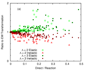
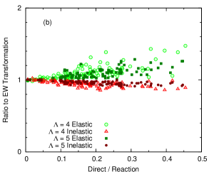
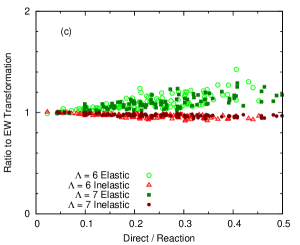
Figure 1: Ratio of calculated cross sections using randomly generated $S$-matrix, as a function of the direct reaction strength. The ratio is that of generalized transmission coefficient calculations to the EW transformation case. The top panel (a) is for a number of channels of $\Lambda=2$ and 3, the middle panel (b) is for $\Lambda=4$ and 5, and the bottom panel (c) is for $\Lambda=6$ and 7.

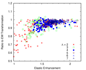
Figure 2: Ratio of calculated inelastic scattering cross section with the generalized transmission coefficient calculations to the EW transformation case, as a function of the elastic enhancement factor $W_{a}$.

III.2 Uncoupled states

To investigate the uncoupled channel in the EW transformation, we construct $S$ with $\Lambda=3$ as in

$$S=\left(\begin{array}[]{ccc}S_{aa}&S_{ba}&\\ S_{ab}&S_{bb}&\\ &&S_{cc}\\ \end{array}\right),$$ (31)

where the channel $c$ is uncoupled to the channels $a$ and $b$. The calculated cross sections with the generalized transmission coefficients are shown by the ratio to the EW transformation in Fig. 3. As opposed to the coupled inelastic scattering channel, the cross section to the uncoupled channel increases very slightly, but is almost not influenced by the channel coupling. This suggests, in the case of neutron-induced reactions on deformed nuclei, that the inelastic scattering cross sections will be enhanced mainly at the expense of the elastic channel, while the neutron capture and fission cross sections will practically not change.

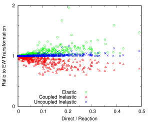
Figure 3: Ratio of the cross sections calculated with the generalized transmission coefficient calculations to the cross sections calculated with EW transformation case, for $\Lambda=3$ and the third channel is uncoupled.

III.3 Simulation for Moldauer’s estimation

Because the term of $\overline{\tilde{S}_{\alpha\alpha}\tilde{S}_{\beta\beta}^{*}}$ in Eq. (15) is a quantity in the diagonalized channel space, we can evaluate this with the GOE triple-integral of Eq. (II.1) whenever $\left\langle{S}\right\rangle$ is diagonal. We replace $\tilde{S}_{\alpha\alpha}$ by $\left\langle{S_{aa}}\right\rangle$, and apply the Monte Carlo technique to calculate $\overline{S_{aa}S_{bb}^{*}}$ by sampling the diagonal $S$-matrix, as well as the number of channels $\Lambda$ that is randomly varied from 2 to 200. We generated 500 such random $S$-matrices, and the calculated $|\overline{S_{aa}S_{bb}^{*}}|$ is shown by the symbols in Fig. 4. When there are many open channels, $\sum_{c}T_{c}\gg 1$, this term will be negligible.

Applying two different estimates for $\nu_{a}$ obtained by Moldauer Moldauer80 and at LANL Kawano14 , Eq. (19) can be evaluated very easily. Figure 5 shows the ratio of Eq. (19) to the GOE results, using two functional forms for $\nu_{a}$. Since $\overline{S_{aa}S_{bb}^{*}}$ is complex due to the factor of $\overline{S_{aa}}\overline{S_{bb}^{*}}$ in Eq. (II.1), the ratio is taken for the absolute value (the module). It can be seen clearly that the updated systematics of $\nu_{a}$ at LANL produces an excellent agreement with GOE, except for in the very small $\sum_{c}T_{c}$ region, where all statistical models tend to fail Kawano14 .

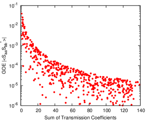
Figure 4: Calculated $|\overline{S_{aa}S_{bb}^{*}}|$ with the GOE triple-integral formula for randomly generated $S$-matrix and number of channels. The results are shown as a function of $\sum_{c}T_{c}$.

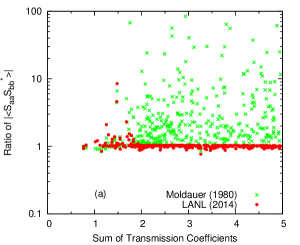
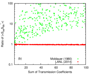
Figure 5: Comparison of Moldauer’s estimate for $|\overline{S_{aa}S_{bb}^{*}|}$ given by Eq. (17) for various $T_{a}$ values and channels, shown by the ratios to the GOE calculation. Two different estimates for the channel degree-of-freedom $\nu$, Refs. Moldauer80 and Kawano14 , are used; the top panel (a) is for smaller $\sum_{c}T_{c}$ case, and the bottom panel (b) is for larger $\sum_{c}T_{c}$ case.

III.4 Simulation for cross section

Our next step is to confirm whether Eq. (15) with the estimation for $\overline{\tilde{S}_{\alpha\alpha}\tilde{S}_{\beta\beta}^{*}}$ in Eq. (19) is a good approximation for the actual cross section calculations. To this end, we calculate the cross sections using the randomly generated non-diagonal $S$-matrix again, and compare with the reference GOE cross sections.

The calculated cross sections for the compound elastic and inelastic channels are shown by the deviation from GOE in Fig. 6, as a function of total cross section $\sigma^{\rm T}$. The standard deviation is 0.83% for the $\Lambda=2$ case, and 0.29% for $\Lambda=5$. From this comparison, we conclude that Moldauer’s model of Eq. (17) with the additional phase factor provides a very good approximation to the GOE triple-integral formula when the off-diagonal elements in the $S$-matrix exist. In reality, because the actual direct channel coupling is much weaker than our randomly generated $S$-matrix, and the number of channels tends to be larger, Eqs (15) and (19) should provide an excellent alternative procedure to calculate compound reaction cross sections, leading to almost identical cross sections as the rigorous GOE formula Nishioka89 .

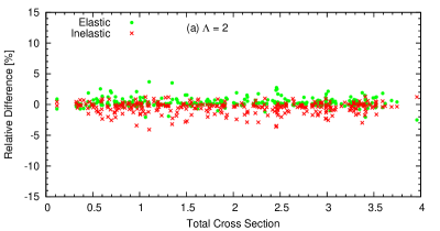
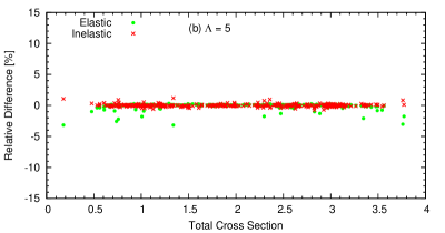
Figure 6: Compound elastic and inelastic cross sections calculated with randomly sampled $S$-matrix as well as using Moldauer’s estimate for $|\overline{\tilde{S}_{\alpha\alpha}\tilde{S}_{\beta\beta}^{*}|}$, as a function of the dimensionless total cross section. The results are shown by the deviation from the GOE results. The top panels are for the two channels case, and the bottom panels are for the five channels.

IV Coupled-channels and Hauser-Feshbach model in a realistic case

We now calculated compound cross sections for neutron induced reactions on ²³⁸U in the fast energy range with the coupled-channels Hauser-Feshbach code CoH₃, and implement the EW transformation as well as all the necessary formulae given previously. Note that the intention here is not to provide the best evaluated cross section, but to study how large the impact of the EW transformation on actual cross section calculations will be. Albeit it is redundant, we summarize here the procedure of cross section calculation including the EW transformation as a practical recipe for applications.

• For a given total spin and parity $J\Pi$, solve the coupled-channels equation. The coupled-channels $S$-matrix is converted into $P$-matrix by Eq. (10), then diagonalized by $UPU^{\dagger}$ to obtain the eigenvalues $p_{\alpha}$ and the eigenvector $U$. We also need the diagonalized $S$-matrix, $\tilde{S}=USU^{T}$.

• Calculate the transmission sum for all open channels as

  $$T=\sum_{\alpha}p_{\alpha}+\sum_{k}T_{k}(\mbox{uncoupled}).$$ (32)

• Calculate the channel cross section matrix in the transformed space

  $$\sigma_{\alpha\beta}=\frac{p_{\alpha}p_{\beta}}{T}W_{\alpha\beta},$$ (33)

  where the width fluctuation factor $W_{\alpha\beta}$ is given by Eq. (4).

• For a set of coupled levels, given a fixed set of incoming ($a$) and outgoing ($b$) channels, sum over $a$ and $b$ when $a\in$ (ground state), and $b\in$ (ground or excited state). Summation $\alpha$ and $\beta$ runs over all the diagonal space, and calculate the cross section as in Eq .(15) with Eqs. (16) and (19).

• For uncoupled levels, run $a$ over the channels that belong to the ground state. The cross section is given by Eq. (21).

We employed the dispersive coupled-channels optical potential by Soukhovitskii et al. Soukhovitskii05 , with the deformation parameters of $\beta_{2}=0.214$, $\beta_{4}=0.00931$, and $\beta_{6}=-0.0148$ taken from the Finite Range Droplet Model Moller95 . We coupled five levels in the ground state rotational band, $0^{+}$, $2^{+}$, $4^{+}$, $6^{+}$, and $8^{+}$. Although direct inelastic scattering to the vibrational bands can be observed, we consider them as uncoupled levels to simplify the calculations, otherwise a different optical model would be needed.

The photon strength function is calculated with the Giant Dipole Resonance (GDR) model with the parameters of Ullmann et al. Ullmann14 . The level density of ²³⁹U is calculated with Gilbert and Cameron’s composite formula Gilbert65 ; Kawano06 , and the level density parameter is slightly adjusted to reproduce the average resonance spacing of $D_{0}=20.26\pm 0.72$ eV Mughabghab06 . The fission barrier parameters are taken from Iwamoto’s study Iwamoto07 , and adjusted to roughly reproduce the evaluated fission cross section at 1 MeV in ENDF/B-VII ENDF7 . Note that the fission channel is not important, since we are mainly interested in the cross sections in the sub-threshold fission region.

Figure 7 shows the comparison of calculated inelastic scattering cross sections for the $2^{+}$, $4^{+}$, $6^{+}$, and $8^{+}$ states. The dashed curves are calculated with the generalized transmission coefficients as in Eq. (9). We also depict the evaluated cross sections in JENDL-4 Iwamoto07 ; JENDL4 for comparison, since these cross sections were calculated with a similar optical model with the coupled-channels Hauser-Feshbach code, CCONE Iwamoto07 , in which the generalized transmission coefficients are adopted. The solid curves are the result of EW transformation. The transformation always increases the inelastic scattering cross section to the level that has the direct component, which we already observed in Fig. 1 in the randomly generated $S$-matrix model. Because the compound formation cross section $\sigma^{\rm CN}$ remains the same, the increase in the inelastic channels reduces the enhancement in the compound elastic channel. However, the reduction in the elastic scattering cross section is not so visible, since the shape elastic scattering $\sigma_{\rm SE}$ dominates the elastic channel in this energy range.

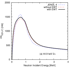
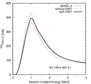
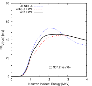
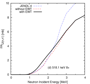
Figure 7: Calculated ²³⁸U(n,n’) reaction cross sections with the EW transformation (solid curves) compared with the modified transmission calculation (dashed curves), as well as with the evaluated cross sections in JENDL-4 (dot-dashed curves).

The calculated capture, total inelastic, and fission cross sections are shown in Fig. 8, as a ratio of the EW transformation case to the generalized transmission case. The total inelastic scattering includes both the coupled and uncoupled levels. As we already saw in Fig. 3, the generalized transmission calculation gives slightly larger cross sections for the uncoupled capture and fission channels. However, the change in these cross sections are less than 2%, while uncertainties in the calculated capture and fission cross sections are much larger in general.

The ratios approach to unity as the neutron incident energy increases, and the impact of the EW transformation disappears above a few MeV. Above that energy, the compound elastic scattering cross section can be basically ignored, because there are many open channels. Under such circumstances the Hauser-Feshbach theory is justified, and the cross sections can be calculated without the EW transformation.

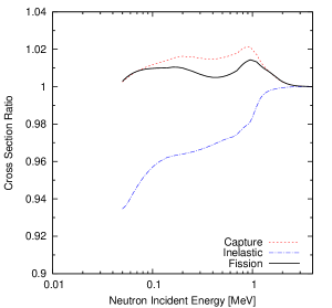
Figure 8: Ratios of calculated capture, total inelastic and fission cross sections without EW transformation to the EW cases.

V Conclusion

An exact formula for the width fluctuation corrected Hauser-Feshbach cross section, in which directly coupled channels are involved, is used to perform the statistical model calculation based on Gaussian Orthogonal Ensemble (GOE) in the diagonalized space — the so-called Engelbrecht-Weidenmüller (EW) transformation. Nishioka, Weidenmüller, and Yoshida Nishioka89 obtained an equivalent expression of the fluctuation cross section without the diagonalization procedure. Nevertheless, the latter has not been employed in practical cross section calculations, due to the complexity both in the formula itself and technical difficulties in applying actual cases. To overcome this problem, we have developed an approximated method, which produces almost identical cross sections as the theory of Nishioka et al., and is feasible to compute cross sections in realistic cases without any of the difficulties the GOE inherently possesses. The method combines Moldauer’s approximation Moldauer75b with a simple relation between the channel degree-of-freedom and the optical model transmission coefficient, recently obtained by a GOE numerical study at LANL Kawano14 .

We have confirmed the Moldauer’s approximation for the first time by our Monte Carlo approach, and found that an extra phase factor should be included when ${\rm Im}(\overline{S}_{\alpha\alpha}\overline{S}_{\beta\beta})\neq 0$. The method was applied to the description of neutron induced reactions on ²³⁸U target in the fast energy range, where the elastic and inelastic scattering, the radiative neutron capture and the fission channels are relevant. We demonstrated that the EW transformation indeed increases the calculated inelastic scattering cross sections, while modest changes were seen in the uncoupled channels, including the fission and capture cross sections. We concluded that conventional methods calculating the Hauser-Feshbach theory by adopting the generalized (direct cross section eliminated) transmission coefficients lead to underestimation of the inelastic scattering cross sections, when the direct channels are strongly coupled. This underestimation decreases as the number of open channels increases. We believe this technique should be adopted by existing Hauser-Feshbach codes, leading to more accurate predictions of the scattering cross sections on collective nuclei.

References

- (1) W. Hauser, H. Feshbach, Phys. Rev. 87, 366 (1952).
- (2) T. Tamura, Rev. Mod. Phys. 37, 679 (1965).
- (3) T. Kawano, P. Talou, J. E. Lynn, M. B. Chadwick, D. G. Madland, Phys. Rev. C 80, 024611 (2009).
- (4) M. W. Herman, R. Capote, B. V. Carlson, P. Oblozinský, M. Sin, A. Trkov, H. Wienke, V. Zerkin, Nucl. Data Sheets 108, 2655 (2007).
- (5) A. J. Koning, S. Hilaire, M. C. Duijvestijn, Proc. Int. Conf. on Nuclear Data for Science and Technology, 22 – 27 Apr., 2007, Nice, France, Ed. O. Bersillon, F. Gunsing, E. Bauge, R. Jacqmin, and S. Leray, EDP Sciences, pp.211–214 (2008).
- (6) O. Iwamoto, J. Nucl. Sci. Technol. 44, 687 (2007).
- (7) T. Kawano, computer code CoH3 [unpublished].
- (8) T. Kawano, P. Talou, M. B. Chadwick, T. Watanabe J. Nucl. Sci. Technol. 47, 462 (2010).
- (9) T. Kawano, P. Talou, H. A. Weidenmüller Phys. Rev. C 92, 044617 (2015).
- (10) M. Kawai, A. K. Kerman, K. W. McVoy, Ann. Phys. 75, 156 (1973).
- (11) G. Arbanas, C. Bertulani, D.J. Dean, A.K. Kerman, Proc. of the 2007 Int. Workshop on Compound-Nuclear Reactions and Related Topics (CNR* 2007), Tenaya Lodge at Yosemite National Park, Fish Camp, California, USA 22-26 October 2007, AIP Conference Proceedings 1005, pp.160–163 Eds. J. Escher, F.S. Dietrich, T. Kawano, I. Thompson (2008).
- (12) T. Kawano, L. Bonneau, A. Kerman, “Effects of direct reaction coupling in compound reactions,” Proc. Int. Conf. on Nuclear Data for Science and Technology, 22 – 27 Apr., 2007, Nice, France, Ed. O. Bersillon, F. Gunsing, E. Bauge, R. Jacqmin, and S. Leray, EDP Sciences, pp.147–150 (2008).
- (13) C. A. Engelbrecht, H. A. Weidenmüller, Phys. Rev. C 8, 859 (1973).
- (14) H. M. Hofmann, J. Richert, J. W. Tepel, H. A. Weidenmüller, Ann. Phys. 90, 403 (1975).
- (15) P. A. Moldauer, Phys. Rev. C 12, 744 (1975).
- (16) H. Nishioka, H.A. Weidenmüller, S. Yoshida, Ann. Phys. 193, 195 (1989).
- (17) J. J. M. Verbaarschot, H. A. Weidenmüller, M. R. Zirnbauer, Phys. Rep. 129, 367 (1985).
- (18) R. Capote, A. Trkov, M. Sin, M. Herman, A. Daskalakis, Y. Danon, Nucl. Data Sheets 118, 26 (2014).
- (19) J. Raynal, computer code ECIS [unpublished].
- (20) T. Kawano, P. Talou, Nuclear Data Sheets 118, 183 (2014).
- (21) J. J. M. Verbaarschot, Ann. Phys. 168, 368 (1986).
- (22) P. A. Moldauer, Phys. Rev. C 11, 426 (1975).
- (23) P. A. Moldauer, Phys. Rev. C 14, 764 (1976).
- (24) P. A. Moldauer, “Statistical Theory of Neutron Nuclear Reactions,” ANL/NDM-40, Argonne National Laboratory (1978).
- (25) S. Hilaire, Ch. Lagrange, A. J. Koning, Ann. Phys. 306, 209 (2003).
- (26) P. A. Moldauer, Nucl. Phys. A, 344, 185 (1980).
- (27) M. Ernebjerg, M. Herman, Proc. Int. Conf. on Nuclear Data for Science and Technology, 26 Sept. – 1 Oct., 2004, Santa Fe, USA, Ed. R.C. Haight, M.B. Chadwick, T. Kawano, and P. Talou, American Institute of Physics, AIP Conference Proceedings 769, p.1233 (2005).
- (28) G. R. Satchler, Phys. Lett. 7, 55 (1963).
- (29) T. Kawano, Eur. Phys. J. A 51,164 (2015).
- (30) E. Sh. Soukhovitskii, R. Capote, J. M. Quesada, S. Chiba, Phys. Rev. C 72, 024604 (2005).
- (31) P. Möller, J. R. Nix, W. D. Myers, W. J. Swiatecki, At. Data and Nucl. Data Tables 59, 185 (1995).
- (32) J. L. Ullmann, T. Kawano, T. A. Bredeweg, A. Couture, R. C. Haight, M. Jandel, J. M. O’Donnell, R. S. Rundberg, D. J. Vieira, J. B. Wilhelmy, J. A. Becker, A. Chyzh, C. Y. Wu, B. Baramsai, G. E. Mitchell, M. Krtička, Phys. Rev. C 89, 034603 (2014).
- (33) A. Gilbert, A. G. W. Cameron, Can. J. Phys., 43, 1446 (1965).
- (34) T. Kawano, S. Chiba, H. Koura, J. Nucl. Sci. Technol., 43, 1 (2006); T. Kawano, “updated parameters based on RIPL-3,” (unpublished, 2009).
- (35) S. F. Mughabghab, “Atlas of Neutron Resonances, Resonance Parameters and Thermal Cross Sections, Z=1–100,” Elsevier (2006).
- (36) M. B. Chadwick, M. Herman, P. Obložinský, M.E. Dunn, Y. Danon, A.C. Kahler, D.L. Smith, B. Pritychenko, G. Arbanas, R. Arcilla, R. Brewer, D.A. Brown, R. Capote, A.D. Carlson, Y.S. Cho, H. Derrien, K. Guber, G.M. Hale, S. Hoblit, S. Holloway, T.D. Johnson, T. Kawano, B.C. Kiedrowski, H. Kim, S. Kunieda, N.M. Larson, L. Leal, J.P. Lestone, R.C. Little, E.A. McCutchan, R.E. MacFarlane, M. MacInnes, C.M. Mattoon, R.D. McKnight, S.F. Mughabghab, G.P.A. Nobre, G. Palmiotti, A. Palumbo, M.T. Pigni, V.G. Pronyaev, R.O. Sayer, A.A. Sonzogni, N.C. Summers, P. Talou, I.J. Thompson, A. Trkov, R.L. Vogt, S.C. van der Marck, A. Wallner, M.C. White, D. Wiarda, P.G. Young Nuclear Data Sheets 112, 2887 (2011).
- (37) K. Shibata, O. Iwamoto, T. Nakagawa, N. Iwamoto, A. Ichihara, S. Kunieda, S. Chiba, K. Furutaka, N. Otuka, T. Ohsawa, T. Murata, H. Matsunobu, A. Zukeran, S. Kamada, J. Katakura, J. Nucl. Sci. Technol. 48, 1 (2011).