Semi-implicit anisotropic cosmic ray transport on an unstructured moving mesh

Abstract

In the interstellar medium of galaxies and the intracluster gas of galaxy clusters, the charged particles making up cosmic rays are moving almost exclusively along (but not across) magnetic field lines. The resulting anisotropic transport of cosmic rays in the form of diffusion or streaming not only affects the gas dynamics but also rearranges the magnetic fields themselves. The coupled dynamics of magnetic fields and cosmic rays can thus impact the formation and evolution of galaxies and the thermal evolution of galaxy clusters in critical ways. Numerically studying these effects requires solvers for anisotropic diffusion that are accurate, efficient, and robust, requirements that have proven difficult to satisfy in practice. Here, we present an anisotropic diffusion solver on an unstructured moving mesh that is conservative, does not violate the entropy condition, allows for semi-implicit time integration with individual timesteps, and only requires solving a single linear system of equations per timestep. We apply our new scheme to a large number of test problems and show that it works as well or better than previous implementations. Finally, we demonstrate for a numerically demanding simulation of the formation of an isolated disk galaxy that our local time-stepping scheme reproduces the results obtained with global time-stepping at a fraction of the computational cost.

1 Introduction

Energetic particles carry a significant fraction of the free energy in the Universe. Their acceleration, their interactions, and their eventual fate are integral parts of the evolution of astrophysical systems such as galaxies, galaxy clusters, and the intergalactic medium that fills the space in between. Particle accelerators for these charged, relativistic particles, called cosmic rays (CRs), are strong shocks, forming for example when a star explodes as a supernova, when a black-hole system ejects matter at relativistic velocities, or when galaxy clusters collide (Blandford & Eichler, 1987). In the interstellar medium (ISM), shocks at supernova remnants are able to accelerate a tiny fraction of $\sim 10^{-9}$ particles to relativistic energies so that the resulting population of CRs collects on average an equal share of the total energy stored in thermal particles, turbulence, and magnetic fields (Boulares & Cox, 1990).

The processes that determine the energy and spatial distribution of CRs are different from those that shape collisional gases, because they rely almost entirely on electric and magnetic fields: the CR particle mean free path due to collisional processes (which are dominated by hadronic interactions with the ambient gas at relativistic CR energies) is $\lambda_{\mathrm{had}}\sim 10\,n_{\mathrm{cm}^{-3}}^{-1}\,\mathrm{Mpc}$ and thus much larger than any relevant scale in galaxies or clusters (Pfrommer & Enßlin, 2004). The potential wells of galaxies ($1$ to $100$ eV) and galaxy clusters ($1$ to $10$ keV) would be too shallow to keep relativistic particles bound if they could move freely along straight lines. The escape time of CRs from the ISM of the Galaxy is however quite long, of order $3\times 10^{7}$ yr. Also, the observed spatial isotropy of CRs (Schlickeiser, 2002; Kulsrud, 2005) suggests the existence of a very efficient scattering mechanism that isotropises their distribution.

These scattering processes support a kind of self-organisation that, through interactions between particles and electromagnetic fields, arranges the particles and the available energy into three components: a cool or warm gas phase that carries the bulk of the mass, energetic particles with a wide range of energies, and a turbulent electromagnetic field that links the two. CRs streaming along the magnetic field excite resonant Alfvén waves through the ‘streaming instability’ (Lerche, 1967; Kulsrud & Pearce, 1969; Skilling, 1971). As a result, the CRs experience rapid pitch-angle scatterings with this wave field, which causes an isotropization of their distribution in the frame of the Alfvén waves, thereby limiting the CR bulk speed to the Alfvén velocity. In addition, CRs can diffuse relative to this wave frame, as well as across field lines by scattering off magneto-hydrodynamic (MHD) turbulence (Wiener et al., 2013).

However, interactions with Alfvén modes of the cascade are extremely inefficient due to the increasing anisotropy at small scales, with power concentrated in modes with wave-vectors transverse to the magnetic field, while CRs efficiently scatter off the parallel component (Chandran, 2000; Yan & Lazarian, 2002). Fast magnetosonic modes could potentially scatter CRs more efficiently (Yan & Lazarian, 2004; Brunetti & Lazarian, 2007), but this process is thought to be a small effect (Desiati & Zweibel, 2014) so that CRs are transported almost entirely along magnetic field lines, giving rise to strongly anisotropic CR transport.

What is the observational evidence for anisotropic CR transport? Observations of polarised radio emission from edge-on galaxies show poloidal field lines at the interface of the galactic disk and halo (e.g., Tüllmann et al., 2000), which corresponds to the location from where galactic winds are launched. This argues for a dynamical mechanism that is able to reorient the preferentially toroidal field in galactic disks by means of anisotropic CR transport along the magnetic field. If CR energy is injected into the ISM by diffusive shock acceleration at supernova remnants, the light CR components finds itself underneath the mass-carrying thermal phase of the ISM. As a consequence, CRs attempt to buoyantly rise from the disk and drive a Parker instability (Rodrigues et al., 2016). As they are dragging the magnetic field with them, this eventually results in a poloidal (‘open’) field configuration.

In recent years, different groups have started to incorporate CR transport into simulations of galaxy formation and evolution and simulations of the ISM. Simulations of the formation of isolated disk galaxies have demonstrated the presence of strong CR-driven outflows by following isotropic (Uhlig et al., 2012) or anisotropic (Ruszkowski et al., 2016) CR streaming as the active transport mechanism for CRs. It was also demonstrated that isotropic CR diffusion can drive galactic winds in isolated Milky Way-sized disk galaxies (Booth et al., 2013; Salem & Bryan, 2014). Moreover, this result still holds for a simulated galaxy that forms in a cosmological environment (Salem et al., 2014). On smaller scales, simulations of the ISM that account for anisotropic CR diffusion demonstrate the launch of strong winds from the disk (Hanasz et al., 2013; Girichidis et al., 2016).

All these simulations employ an explicit time integration scheme. This severely limits the achievable resolution since the timestep constraint of explicit schemes for CR diffusion scales quadratically with linear dimensions of a resolution element. Thus, it is desirable to develop semi-implicit or implicit time-integration schemes in order to avoid a very restrictive timestep limitation of the diffusion solver.

Moreover, Sharma & Hammett (2007) recently analysed the numerical properties of discretisation schemes for anisotropic heat conduction (which exhibit the same mathematical properties as anisotropic diffusion) and demonstrated that they generally violate the entropy condition $\Delta S\geq 0$, i.e., heat can be transported from cold to warm regions (or equivalently CRs are transported from regions of low to high abundance), unless this behaviour is not explicitly prevented by an ingenious design of the numerical scheme. Unfortunately, anisotropic diffusion schemes that do not violate the entropy condition introduce non-linearities that significantly increase the numerical complexity when one tries to combine them with an efficient implicit time integrator, although efficient semi-implicit schemes are still possible (Sharma & Hammett, 2011; Kannan et al., 2016; Hopkins, 2016).

Of particular importance for multi-scale problems such as galaxy evolution is another issue that arises for implicit time integration schemes from the coupling to the dynamics of the magnetic field. To take the dynamics of the magnetic field accurately into account in the diffusion solver, the diffusion problem for every cell (or particle) has to be integrated on a timestep smaller or equal to its MHD timestep. Thus, integrating the diffusion solver on global timesteps requires a reduction of the global timestep to the smallest MHD timestep in the simulation, rendering large, multi-scale problems to become almost impossible. To avoid this impasse, we must develop a method that allows for individual timesteps, i.e., it needs to tolerate different diffusion timesteps for each cell chosen on local conditions, while at the same time guaranteeing stability for timesteps that are much larger than those required by the stability criterion of explicit time integration of the diffusion problem. Such a scheme has been proposed by Dubois & Commerçon (2016), however, their algorithm does not ensure energy conservation and in general violates the entropy condition.

Here, we discuss a novel anisotropic diffusion scheme implemented in the moving-mesh code arepo (Springel, 2010). It is based on the flux limiting scheme by Sharma & Hammett (2007) and the semi-implicit time-integration scheme presented by Sharma & Hammett (2011), with some refinements. In particular, we generalise the scheme to unstructured meshes and extend it to allow for semi-implicit time integration with individual timesteps while still ensuring energy conservation and preserving the entropy condition. The present paper concentrates on the technical treatment of the CR diffusion problem, while a companion paper (Pfrommer et al., 2016) describes the foundations of the CR physics implemented in the code, focusing in particular on the source and sink processes. In two further companion papers, we apply our new methods to wind formation in disk galaxies (Pakmor et al., 2016b) and to the effects of individual supernova explosions in the ISM (Simpson et al., 2016).

This paper is structured as follows. We first describe our algorithm and implementation in Section 2. We then apply it to several common test problems in Section 3 and show that the implicit individual time-stepping delivers exquisite results for the problem of the formation of an isolated disk galaxy in Section 4. Finally, we summarise our results in Section 5.

2 Implementation

The part of the evolution equation for the CR energy density $\varepsilon_{\mathrm{cr}}$ that describes anisotropic diffusion is given by

$$\frac{\partial\varepsilon_{\mathrm{cr}}}{\partial t}-\bm{\nabla}\mathchoice{\mskip 3.0mu\lower 0.86108pt\hbox{\scalebox{1.5}{$\cdot$}}\mskip 3.0mu}{\mskip 3.0mu\lower 0.86108pt\hbox{\scalebox{1.5}{$\cdot$}}\mskip 3.0mu}{\lower 1.29167pt\hbox{\scalebox{1.2}{$\cdot$}}}{\lower 1.29167pt\hbox{\scalebox{1.2}{$\cdot$}}}\left[\kappa_{\varepsilon}\textbf{{b}}\left(\textbf{{b}}\mathchoice{\mskip 3.0mu\lower 0.86108pt\hbox{\scalebox{1.5}{$\cdot$}}\mskip 3.0mu}{\mskip 3.0mu\lower 0.86108pt\hbox{\scalebox{1.5}{$\cdot$}}\mskip 3.0mu}{\lower 1.29167pt\hbox{\scalebox{1.2}{$\cdot$}}}{\lower 1.29167pt\hbox{\scalebox{1.2}{$\cdot$}}}\bm{\nabla}\varepsilon_{\mathrm{cr}}\right)\right]=0,$$ (1)

where $\varepsilon_{\mathrm{cr}}$ is the CR energy density, $\kappa_{\varepsilon}$ is the kinetic energy-weighted diffusion coefficient, and $\textbf{{b}}=\textbf{{B}}/\left|\textbf{{B}}\right|$ is the direction of the magnetic field. The full evolution equation for the CR energy density includes terms to describe the acceleration, the advection, and the cooling of CRs (Pfrommer et al., 2016). Here, we concentrate only on the diffusion term; the other terms are effectively treated in an operator split fashion by the code.

After integrating the diffusion term over the volume $V_{i}$ of cell $i$, applying Gauss’ theorem to the divergence term, and dividing by the cell volume, we obtain

$$\frac{\partial\varepsilon_{\mathrm{cr},i}}{\partial t}-\frac{1}{V_{i}}\int_{\partial V_{i}}\kappa_{\varepsilon}\left(\textbf{{b}}\mathchoice{\mskip 3.0mu\lower 0.86108pt\hbox{\scalebox{1.5}{$\cdot$}}\mskip 3.0mu}{\mskip 3.0mu\lower 0.86108pt\hbox{\scalebox{1.5}{$\cdot$}}\mskip 3.0mu}{\lower 1.29167pt\hbox{\scalebox{1.2}{$\cdot$}}}{\lower 1.29167pt\hbox{\scalebox{1.2}{$\cdot$}}}\bm{\nabla}\varepsilon_{\mathrm{cr}}\right)\textbf{{b}}\mathchoice{\mskip 3.0mu\lower 0.86108pt\hbox{\scalebox{1.5}{$\cdot$}}\mskip 3.0mu}{\mskip 3.0mu\lower 0.86108pt\hbox{\scalebox{1.5}{$\cdot$}}\mskip 3.0mu}{\lower 1.29167pt\hbox{\scalebox{1.2}{$\cdot$}}}{\lower 1.29167pt\hbox{\scalebox{1.2}{$\cdot$}}}\mathrm{d}\textbf{{A}}_{i}=0.$$ (2)

Here, $\varepsilon_{\mathrm{cr},i}$ is the CR energy density in cell $i$ and $\mathrm{d}\textbf{{A}}_{i}$ points along the normal vector of the surface.

Discretization of the surface integral leads to

$$\frac{\partial\varepsilon_{\mathrm{cr},i}}{\partial t}-\frac{1}{V_{i}}\sum_{j}\kappa_{ij}\left(\textbf{{b}}_{ij}\mathchoice{\mskip 3.0mu\lower 0.86108pt\hbox{\scalebox{1.5}{$\cdot$}}\mskip 3.0mu}{\mskip 3.0mu\lower 0.86108pt\hbox{\scalebox{1.5}{$\cdot$}}\mskip 3.0mu}{\lower 1.29167pt\hbox{\scalebox{1.2}{$\cdot$}}}{\lower 1.29167pt\hbox{\scalebox{1.2}{$\cdot$}}}\bm{\nabla}\varepsilon_{\mathrm{cr},ij}\right)\textbf{{b}}_{ij}\mathchoice{\mskip 3.0mu\lower 0.86108pt\hbox{\scalebox{1.5}{$\cdot$}}\mskip 3.0mu}{\mskip 3.0mu\lower 0.86108pt\hbox{\scalebox{1.5}{$\cdot$}}\mskip 3.0mu}{\lower 1.29167pt\hbox{\scalebox{1.2}{$\cdot$}}}{\lower 1.29167pt\hbox{\scalebox{1.2}{$\cdot$}}}\textbf{{n}}_{ij}A_{ij}=0.$$ (3)

This sum runs over all interfaces $j$ of cell $i$ and depends on the diffusion coefficient $\kappa_{ij}$, the direction of the magnetic field $\textbf{{b}}_{ij}$, the gradient of the CR energy density $\bm{\nabla}\varepsilon_{\mathrm{cr},ij}$ at the interface, the normal vector $\textbf{{n}}_{ij}$ of the interface and its area $A_{ij}$. Note that for the simpler case of isotropic diffusion the equation becomes

$$\frac{\partial\varepsilon_{\mathrm{cr},i}}{\partial t}-\frac{1}{V_{i}}\sum_{j}\kappa_{ij}\left(\bm{\nabla}\varepsilon_{\mathrm{cr},ij}\mathchoice{\mskip 3.0mu\lower 0.86108pt\hbox{\scalebox{1.5}{$\cdot$}}\mskip 3.0mu}{\mskip 3.0mu\lower 0.86108pt\hbox{\scalebox{1.5}{$\cdot$}}\mskip 3.0mu}{\lower 1.29167pt\hbox{\scalebox{1.2}{$\cdot$}}}{\lower 1.29167pt\hbox{\scalebox{1.2}{$\cdot$}}}\textbf{{n}}_{ij}\right)A_{ij}=0.$$ (4)

To evaluate the sum in Eq. (3) we need an estimate of the full gradient of the CR energy density at every interface. Unfortunately, a naïve estimate of this gradient can lead to unphysical solutions, as one can easily construct situations where the energy can flow from a cell with lower energy density to a cell with higher energy density. One way to avoid this unphysical solution is to limit the gradient appropriately, as described by Sharma & Hammett (2007) for a Cartesian mesh. We follow a similar strategy for tackling this problem, but one that is generalized for an unstructured, Voronoi mesh.

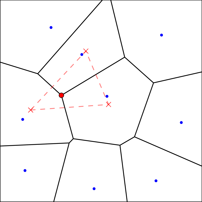
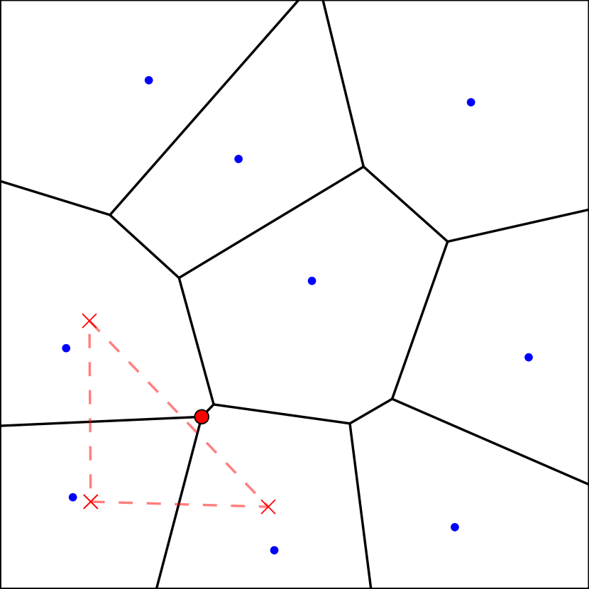
Figure 1: Visualisation of the gradient estimate at a corner of the Voronoi mesh in 2D. Blue circles show the positions of the mesh-generating points, black lines show the edges of the Voronoi cells. The red circle in each panel shows a selected corner whose gradient estimate is based on the values at the centers of mass of the three adjacent cells marked by red crosses. The left panel shows a well-behaved configuration, i.e. the corner lies within the triangle spanned by the three centers of mass. In contrast, the right panel shows an ill-behaved configuration for which the desired interpolation turns into an extrapolation because the corner lies outside the triangle.

2.1 Estimating the gradient at a corner

Similar to Günter et al. (2005) and Sharma & Hammett (2007), we build the gradient estimate at the center of an interface based on gradient estimates of its corners. Thus, we start with gradient estimates at the corners of the Voronoi mesh. In 2D, every corner of a Voronoi mesh connects three cells. The mesh-generating points of these cells create a triangle whose circumcircle center is the position of the corner. To estimate the gradient of a quantity at the corner, we use its values at the centers of mass of the three adjacent cells as sketched in Fig. 1 and perform a least squares fit on the value of the quantity and its gradient at the corner.

In 3D, the triangle becomes a tetrahedron and every corner has four adjacent cells. The residuals of the fit are given by

$$r_{i}=\phi\left(\textbf{{c}}\right)+\left(\bm{\nabla}\phi\right)\left(\textbf{{s}}_{i}-\textbf{{c}}\right)-\phi\left(\textbf{{s}}_{i}\right),$$ (5)

where $\phi\left(\textbf{{c}}\right)$ is the unknown value at the position of the corner c, $\bm{\nabla}\phi$ is the gradient at the corner, and $\phi\left(\textbf{{s}}_{i}\right)$ is the value at the center $\textbf{{s}}_{i}$ of cell $i$. We can rewrite this in the form of a matrix equation

$$\textbf{{r}}=\textbf{{X}}\textbf{{q}}-\textbf{{Y}}.$$ (6)

Here, r, q, and Y are N-vectors with $N=3$ ($N=4$), and X is a $N\times N$ square matrix in 2D (3D). They are defined as

$$(\textbf{{q}})_{0} = \phi\left(\textbf{{c}}\right)$$

$$(\textbf{{q}})_{1..N-1} = \left(\bm{\nabla}\phi\right)_{0..N-2}$$

$$(\textbf{{Y}})_{i} = \phi\left(\textbf{{s}}_{i}\right)$$

$$(\textbf{{X}})_{i,0} = 1$$

$$(\textbf{{X}})_{i,1..N-2} = \textbf{{s}}_{i,0..N-2}-\textbf{{c}}_{0..N-2}.$$

To minimize the residual we solve the normal equations and find

$$\left(\textbf{{X}}^{T}\ \textbf{{X}}\right)\textbf{{q}}=\textbf{{X}}^{T}\ \textbf{{Y}}.$$ (7)

Since X is a square matrix, there is a unique solution for q with zero residual. To solve for q we multiply with $\left(\textbf{{X}}^{T}\ \textbf{{X}}\right)^{-1}$ from the left and obtain

$$${{q}}$=\textbf{{M}}\ \textbf{{Y}},$$ (8)

with $\textbf{{M}}=\left(\textbf{{X}}^{T}\ \textbf{{X}}\right)^{-1}\ \textbf{{X}}^{T}$. Note that M only depends on the geometry of the mesh and Y only contains values at the centers of cells. Thus, we only have to compute M once in every timestep because the geometry of the mesh does not change and can obtain the value and gradient of any quantity at a corner from a simple matrix-vector multiplication. Moreover, Eq. (8) describes the linear dependence of the gradient at the corner on the values in the adjacent cells. This is needed later on for the implicit time integration.

The value of a quantity at the corner only depends on the entries in the first row of M. If the corner lies inside the triangle (tetrahedron) spanned by the centers of mass of the adjacent cells, all values in the first row of M are positive and the value of a quantity at the corner is interpolated from the values at the centers of the adjacent cells. However, as demonstrated in Fig. 1, for general mesh geometries it is possible that the corner lies outside the triangle (tetrahedron). In this case, at least one of the entries in the first row of M is negative and the interpolation becomes an extrapolation, which can in general be unstable. To deal with this we mark any corner as problematic which has an entry in the first row of $\textbf{{M}}_{0,j}<-0.01$ and treat these corners in a special way, as described in Section 2.3. One might consider aggressively setting this threshold to zero, thus not allowing for any extrapolation at the corners at all. However this turns out to increase the diffusivity of the scheme perpendicular to the magnetic field vector and does not seem to be necessary for any of our test problems.

2.2 Calculating the direction of the magnetic field at the interface

The least squares fit estimate of the gradient at the corners also allows us to compute the value of a quantity at the position of a corner. To then obtain a single value for the interface, we perform a weighted average of these values at the corners,

$$\phi_{\mathrm{face}}=\sum_{i}w_{i}\phi\left(\textbf{{c}}_{i}\right).$$ (9)

The weights are set to

$$w_{i}=\frac{A_{i}}{A_{\mathrm{face}}},$$ (10)

where $A_{\mathrm{face}}$ is the area of a face, and $A_{i}$ the area of a tetrahedron defined by the position of the corner, the center of the face, and the two midpoints of the two adjacent edges of the corners that are part of the face (see Fig. 2). In 2D, this simplifies to $w_{i}=0.5$ for both corners of an interface.

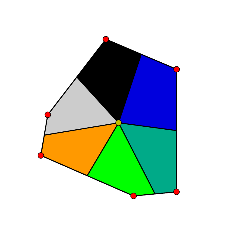
Figure 2: Sketch of the geometric weights with which the different corners contribute to the value of the magnetic field and other quantities at the center of the interface in 3D. The red circles are the corners of the interface, the yellow circle shows the position of the center of the interface, and the size of the coloured areas is proportional to the weight that is associated with the corners.

2.3 Computing the flux

To compute the flux over an interface as given by Eq. (3) we rotate the coordinate system so that one axis points along the normal vector of the interface, one axis points along the magnetic field direction in the interface, and the third axis is perpendicular to the first two, while lying in the interface. We then split the gradient of the CR energy density at the interface into two components: one along the normal direction of the interface and the other in the plane of the interface. In 3D, the latter in principle is a two-dimensional vector. However, we rotate the tangential component in the interface such that one component points along the magnetic field in the interface, and ignore the remaining component that is in the interface but perpendicular to the magnetic field vector and therefore always exactly zero. Thus we can write the split in 2D and in 3D as

$$\bm{\nabla}\varepsilon_{\mathrm{cr}}=\bm{\nabla}\varepsilon_{\mathrm{cr}\mathrm{,n}}+\bm{\nabla}\varepsilon_{\mathrm{cr}\mathrm{,t}}.$$ (11)

We then compute two separate fluxes from them, which add up to the total flux.

We can prevent unphysical fluxes from a cell with lower CR energy density to a cell with higher CR energy density by limiting the gradient on the interface (Sharma & Hammett, 2007). We use a generalized version of the van-Leer limiter (van Leer, 1984) to compute the limited gradient estimate $\bm{\nabla}\varepsilon_{\mathrm{cr}\mathrm{,t}}$ along the magnetic field direction in an interface from the unlimited gradients in the same direction $\bm{\nabla}\varepsilon^{i}_{\mathrm{cr}\mathrm{,t}}$ at corner $i$. If all values of $\bm{\nabla}\varepsilon^{i}_{\mathrm{cr}\mathrm{,t}}$ have the same sign, we calculate $\bm{\nabla}\varepsilon_{\mathrm{cr}\mathrm{,t}}$ by

$$\bm{\nabla}\varepsilon_{\mathrm{cr}\mathrm{,t}}=\frac{N}{\sum_{i}\left(\bm{\nabla}\varepsilon^{i}_{\mathrm{cr}\mathrm{,t}}\right)^{-1}}.$$ (12)

If they do not all have the same sign, we set $\bm{\nabla}\varepsilon_{\mathrm{cr}\mathrm{,t}}=0$.

The gradient estimate includes all corners of the interface except for the ones we previously marked as problematic because their gradient estimate became an extrapolation, as described in detail in Section 2.1. Knowing $\bm{\nabla}\varepsilon_{\mathrm{cr}\mathrm{,t}}$ we can directly compute its associated flux. In the rare case that all corners of an interface are flagged, we use the stricter minmod limiter instead and include all corners.

We implement two different ways to compute the gradient of the CR energy density along the normal direction of the interface. We refer to them as simple normal gradients and full normal gradients. The simple normal gradient estimate only takes the values at centers of mass of the two adjacent cells of an interface into account. From those, we compute a one-dimensional gradient along the connecting line between the two centers (L,R) and project it onto the normal vector of the interface. The gradient estimate is then given by

$$\bm{\nabla}\varepsilon_{\mathrm{cr}\mathrm{,n}}=\frac{\varepsilon_{\mathrm{CR,L}}-\varepsilon_{\mathrm{CR,R}}}{\left|\textbf{{c}}_{L}-\textbf{{c}}_{R}\right|}\left(\frac{\textbf{{c}}_{L}-\textbf{{c}}_{R}}{\left|\textbf{{c}}_{L}-\textbf{{c}}_{R}\right|}\right)\mathchoice{\mskip 3.0mu\lower 0.86108pt\hbox{\scalebox{1.5}{$\cdot$}}\mskip 3.0mu}{\mskip 3.0mu\lower 0.86108pt\hbox{\scalebox{1.5}{$\cdot$}}\mskip 3.0mu}{\lower 1.29167pt\hbox{\scalebox{1.2}{$\cdot$}}}{\lower 1.29167pt\hbox{\scalebox{1.2}{$\cdot$}}}\textbf{{n}}_{\mathrm{face}}.$$ (13)

If the centers of mass of the two cells are at the same position as their mesh-generating points, this estimate is quite accurate because the normal vector of the interface is parallel to the connecting line between the two mesh-generating points. However, in general there is a small deviation between the mesh-generating point and the center of mass of a cell. In this case, the simple normal gradient estimate slightly underestimates the true normal gradient at the interface.

For the full normal gradient estimate on an interface we again make use of the gradient estimates at its corners. We use the same averaging procedure for the normal components of the corner gradients that we use for the magnetic field values at the interface (see Eq. 9). However, here we ignore the contributions of all corners that have been flagged as problematic and replace their contribution to the total sum with the simple gradient estimate.

We do not need to limit the simple normal gradients, because they ensure the entropy condition by construction. When we use full normal gradients, we check for every interface if the direction of the normal gradient given the current CR energy densities of the surrounding cells violates the entropy condition. If that is the case, we use the simple normal gradient estimate instead for this interface.

Note that both estimates of the normal component of the gradient are linear in their dependence on the CR energy densities of the cells. However, for the full gradient estimate the normal component of the gradient for an interface usually depends on the values of a dozen cells or more. In comparison, the simple gradient estimate for an interface only depends on two cells.

2.4 Time integration

We implement two different time integration schemes for anisotropic diffusion, a purely explicit scheme and a semi-implicit scheme. For the explicit time integration, the update is done in two half-steps

$$\varepsilon_{\mathrm{cr},i}^{n+1/2}=\varepsilon_{\mathrm{cr},i}^{n} +\frac{\Delta t}{2V_{i}}\left[\sum_{j}\kappa_{ij}\left(\textbf{{b}}_{ij}\mathchoice{\mskip 3.0mu\lower 0.86108pt\hbox{\scalebox{1.5}{$\cdot$}}\mskip 3.0mu}{\mskip 3.0mu\lower 0.86108pt\hbox{\scalebox{1.5}{$\cdot$}}\mskip 3.0mu}{\lower 1.29167pt\hbox{\scalebox{1.2}{$\cdot$}}}{\lower 1.29167pt\hbox{\scalebox{1.2}{$\cdot$}}}\bm{\nabla}\varepsilon_{\mathrm{CR,t,}ij}^{n}\right)\textbf{{b}}_{ij}\mathchoice{\mskip 3.0mu\lower 0.86108pt\hbox{\scalebox{1.5}{$\cdot$}}\mskip 3.0mu}{\mskip 3.0mu\lower 0.86108pt\hbox{\scalebox{1.5}{$\cdot$}}\mskip 3.0mu}{\lower 1.29167pt\hbox{\scalebox{1.2}{$\cdot$}}}{\lower 1.29167pt\hbox{\scalebox{1.2}{$\cdot$}}}\textbf{{n}}_{ij}A_{ij}\right.$$ (14)

$$+\left.\sum_{j}\kappa_{ij}\left(\textbf{{b}}_{ij}\mathchoice{\mskip 3.0mu\lower 0.86108pt\hbox{\scalebox{1.5}{$\cdot$}}\mskip 3.0mu}{\mskip 3.0mu\lower 0.86108pt\hbox{\scalebox{1.5}{$\cdot$}}\mskip 3.0mu}{\lower 1.29167pt\hbox{\scalebox{1.2}{$\cdot$}}}{\lower 1.29167pt\hbox{\scalebox{1.2}{$\cdot$}}}\bm{\nabla}\varepsilon_{\mathrm{CR,n,}ij}^{n}\right)\textbf{{b}}_{ij}\mathchoice{\mskip 3.0mu\lower 0.86108pt\hbox{\scalebox{1.5}{$\cdot$}}\mskip 3.0mu}{\mskip 3.0mu\lower 0.86108pt\hbox{\scalebox{1.5}{$\cdot$}}\mskip 3.0mu}{\lower 1.29167pt\hbox{\scalebox{1.2}{$\cdot$}}}{\lower 1.29167pt\hbox{\scalebox{1.2}{$\cdot$}}}\textbf{{n}}_{ij}A_{ij}\right],$$

$$\varepsilon_{\mathrm{cr},i}^{n+1}=\varepsilon_{\mathrm{cr},i}^{n+1/2} +\frac{\Delta t}{2V_{i}}\left[\sum_{j}\kappa_{ij}\left(\textbf{{b}}_{ij}\mathchoice{\mskip 3.0mu\lower 0.86108pt\hbox{\scalebox{1.5}{$\cdot$}}\mskip 3.0mu}{\mskip 3.0mu\lower 0.86108pt\hbox{\scalebox{1.5}{$\cdot$}}\mskip 3.0mu}{\lower 1.29167pt\hbox{\scalebox{1.2}{$\cdot$}}}{\lower 1.29167pt\hbox{\scalebox{1.2}{$\cdot$}}}\bm{\nabla}\varepsilon_{\mathrm{CR,t,}ij}^{n+1/2}\right)\textbf{{b}}_{ij}\mathchoice{\mskip 3.0mu\lower 0.86108pt\hbox{\scalebox{1.5}{$\cdot$}}\mskip 3.0mu}{\mskip 3.0mu\lower 0.86108pt\hbox{\scalebox{1.5}{$\cdot$}}\mskip 3.0mu}{\lower 1.29167pt\hbox{\scalebox{1.2}{$\cdot$}}}{\lower 1.29167pt\hbox{\scalebox{1.2}{$\cdot$}}}\textbf{{n}}_{ij}A_{ij}\right.$$

$$+\left.\sum_{j}\kappa_{ij}\left(\textbf{{b}}_{ij}\mathchoice{\mskip 3.0mu\lower 0.86108pt\hbox{\scalebox{1.5}{$\cdot$}}\mskip 3.0mu}{\mskip 3.0mu\lower 0.86108pt\hbox{\scalebox{1.5}{$\cdot$}}\mskip 3.0mu}{\lower 1.29167pt\hbox{\scalebox{1.2}{$\cdot$}}}{\lower 1.29167pt\hbox{\scalebox{1.2}{$\cdot$}}}\bm{\nabla}\varepsilon_{\mathrm{CR,n,}ij}^{n+1/2}\right)\textbf{{b}}_{ij}\mathchoice{\mskip 3.0mu\lower 0.86108pt\hbox{\scalebox{1.5}{$\cdot$}}\mskip 3.0mu}{\mskip 3.0mu\lower 0.86108pt\hbox{\scalebox{1.5}{$\cdot$}}\mskip 3.0mu}{\lower 1.29167pt\hbox{\scalebox{1.2}{$\cdot$}}}{\lower 1.29167pt\hbox{\scalebox{1.2}{$\cdot$}}}\textbf{{n}}_{ij}A_{ij}\right].$$

The two steps are applied at the beginning and at the end of each timestep, respectively. $\varepsilon_{\mathrm{cr},i}^{n}$, $\varepsilon_{\mathrm{cr},i}^{n+1/2}$, and $\varepsilon_{\mathrm{cr},i}^{n+1}$ denote the CR energy density in cell $i$ at the beginning of the timestep, in the middle of the timestep, and at the end of the timestep, respectively.

Moreover, to improve the order of accuracy of the time integration, we first integrate the diffusion term for a half-timestep at the beginning of the timestep, before the first part of the gravity timestep. Later, we integrate it for another half-timestep at the end of the timestep, after the second part of the gravity timestep. Unfortunately, a timestep constraint

$$\Delta t_{\mathrm{diffusion}}<\frac{\Delta x^{2}}{\kappa_{\varepsilon}},$$ (15)

where $\Delta x$ is the diameter of a cell and $\kappa_{\varepsilon}$ the diffusion coefficient in a cell, is required for stability, which severely limits the applicability of the explicit time integration scheme. A common solution to guarantee stability even for large timesteps is to switch to an implicit time integration scheme. However, the limiting procedure for the gradients in the interface makes the system nonlinear and very expensive to solve in a fully implicit scheme.

2.5 Semi-implicit time integration

Fortunately, it is possible to formulate a semi-implicit scheme that is almost as stable as the fully implicit scheme, but only requires solving one linear implicit problem per timestep (Sharma & Hammett, 2011). To achieve this, we split the time integration into two parts. We first advance the CR energy of all cells with the fluxes associated with the components of the CR energy density gradients in the interfaces using an explicit forward Euler time integrator, because the nonlinearity of the tangential gradient estimate $\varepsilon_{\mathrm{CR,t},ij}^{n}$ prohibits an efficient implicit solution, as

$$\varepsilon_{\mathrm{cr},i}^{\tilde{n}}=\varepsilon_{\mathrm{cr},i}^{n}+\frac{\Delta t}{V_{i}}\sum_{j}\kappa_{ij}\left(\textbf{{b}}_{ij}\mathchoice{\mskip 3.0mu\lower 0.86108pt\hbox{\scalebox{1.5}{$\cdot$}}\mskip 3.0mu}{\mskip 3.0mu\lower 0.86108pt\hbox{\scalebox{1.5}{$\cdot$}}\mskip 3.0mu}{\lower 1.29167pt\hbox{\scalebox{1.2}{$\cdot$}}}{\lower 1.29167pt\hbox{\scalebox{1.2}{$\cdot$}}}\bm{\nabla}\varepsilon_{\mathrm{CR,t},ij}^{n}\right)\textbf{{b}}_{ij}\mathchoice{\mskip 3.0mu\lower 0.86108pt\hbox{\scalebox{1.5}{$\cdot$}}\mskip 3.0mu}{\mskip 3.0mu\lower 0.86108pt\hbox{\scalebox{1.5}{$\cdot$}}\mskip 3.0mu}{\lower 1.29167pt\hbox{\scalebox{1.2}{$\cdot$}}}{\lower 1.29167pt\hbox{\scalebox{1.2}{$\cdot$}}}\textbf{{n}}_{ij}A_{ij}.$$ (16)

In a second step, we advance the CR energy of all cells with the fluxes associated with the normal component of the CR energy density gradients at the interfaces that are linear. This is done using an implicit backward Euler scheme:

$$\varepsilon_{\mathrm{cr},i}^{n+1}=\varepsilon_{\mathrm{cr},i}^{\tilde{n}}+\frac{\Delta t}{V_{i}}\sum_{j}\kappa_{ij}\left(\textbf{{b}}_{ij}\mathchoice{\mskip 3.0mu\lower 0.86108pt\hbox{\scalebox{1.5}{$\cdot$}}\mskip 3.0mu}{\mskip 3.0mu\lower 0.86108pt\hbox{\scalebox{1.5}{$\cdot$}}\mskip 3.0mu}{\lower 1.29167pt\hbox{\scalebox{1.2}{$\cdot$}}}{\lower 1.29167pt\hbox{\scalebox{1.2}{$\cdot$}}}\bm{\nabla}\varepsilon_{\mathrm{CR,n},ij}^{n+1}\right)\textbf{{b}}_{ij}\mathchoice{\mskip 3.0mu\lower 0.86108pt\hbox{\scalebox{1.5}{$\cdot$}}\mskip 3.0mu}{\mskip 3.0mu\lower 0.86108pt\hbox{\scalebox{1.5}{$\cdot$}}\mskip 3.0mu}{\lower 1.29167pt\hbox{\scalebox{1.2}{$\cdot$}}}{\lower 1.29167pt\hbox{\scalebox{1.2}{$\cdot$}}}\textbf{{n}}_{ij}A_{ij}.$$ (17)

Since $\bm{\nabla}\varepsilon_{\mathrm{CR,n},ij}^{n+1}$ depends only linearly on the CR energy densities of a set of cells, this constitutes a system of coupled linear equations that can be solved with a matrix solver. We solve the linear system in a two-step procedure using solvers from the hypre library (Falgout & Yang, 2002). We first try to solve the system with the iterative, flexible GMRES solver (Saad & Schultz, 1986) until we either reach a residual smaller than $10^{-8}$ or exceed $200$ iterations. In the latter case, we add an algebraic multigrid preconditioner (Henson & Yang, 2002) to GMRES and iterate until the residual is smaller than $10^{-8}$. This two-step procedure is often significantly faster than using the multigrid preconditioner directly, as the setup phase of the multigrid solver can take more time than $200$ iterations of the pure GMRES solver. Note, however, that for some problems it may be more efficient to always run with the multigrid preconditioner.

Similarly to the findings of Sharma & Hammett (2011), the scheme seems to be stable for very large timesteps, but the result eventually becomes incorrect and the entropy condition can be violated. Moreover, for large diffusion coefficients and large timesteps, significant errors may occur at the timestep boundaries. In practice, this does not happen for cosmic ray diffusion as the cosmic ray diffusion coefficient is somewhat limited, but it may become an issue for certain problems of heat diffusion. If the scheme is applied in such cases, it may require additional constraints on the diffusion timestep.

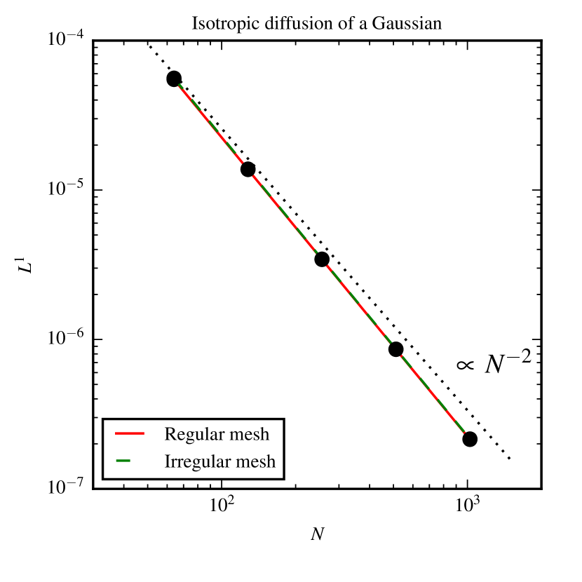
Figure 3: $L^{1}$ norm for isotropic diffusion of a 2D Gaussian profile. The red and green lines show the norm for a regular and an irregular mesh, respectively.

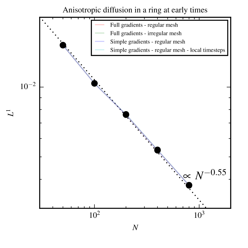
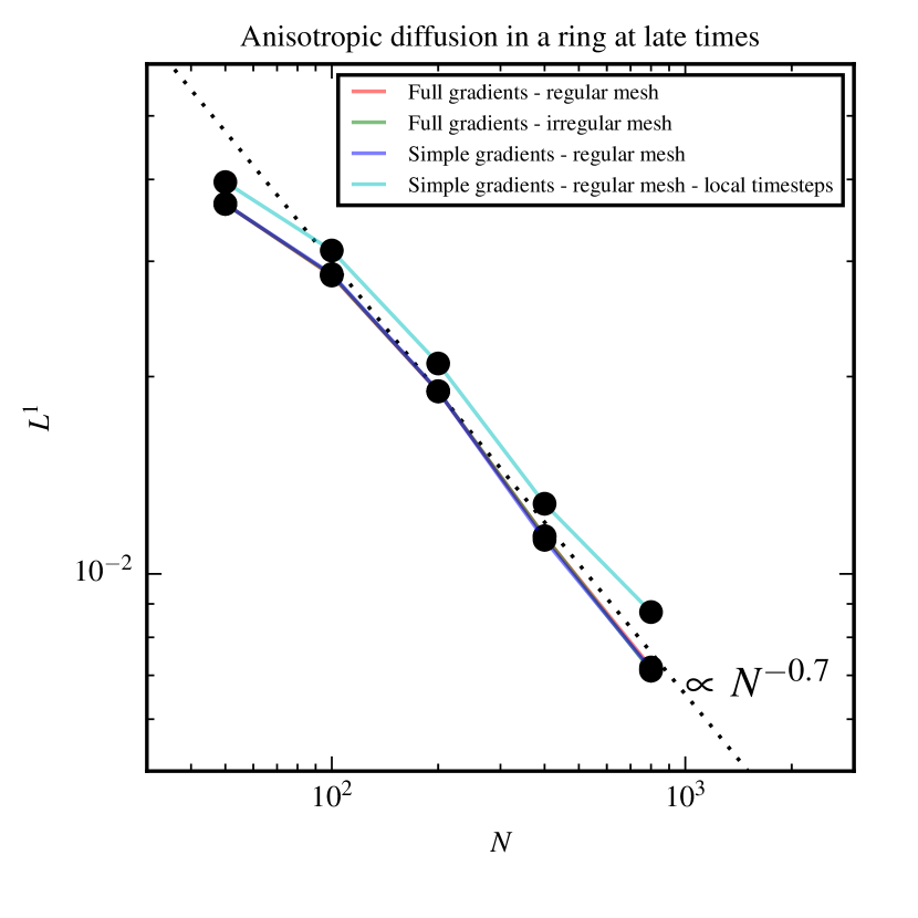
Figure 4: $L^{1}$ norm for anisotropic diffusion of an initial wedge in a circular magnetic field in 2D at times $t=10$ (top panel) and $t=200$ (bottom panel). The solid lines show runs that use different gradient estimates, different meshes, or different time integration schemes, as labelled.

For isotropic diffusion we use a Crank-Nicolson scheme in a similar fashion, i.e. we split the flux into two half-timestep fluxes. We then integrate the first flux explicitly and the second flux implicitly:

$$\varepsilon_{\mathrm{cr},i}^{\tilde{n}} =\varepsilon_{\mathrm{cr},i}^{n}+\frac{\Delta t}{2V_{i}}\sum_{j}\kappa_{ij}\left(\bm{\nabla}\varepsilon_{\mathrm{CR,n},ij}^{n}\mathchoice{\mskip 3.0mu\lower 0.86108pt\hbox{\scalebox{1.5}{$\cdot$}}\mskip 3.0mu}{\mskip 3.0mu\lower 0.86108pt\hbox{\scalebox{1.5}{$\cdot$}}\mskip 3.0mu}{\lower 1.29167pt\hbox{\scalebox{1.2}{$\cdot$}}}{\lower 1.29167pt\hbox{\scalebox{1.2}{$\cdot$}}}\textbf{{n}}_{ij}\right)A_{ij},$$ (18)

$$\varepsilon_{\mathrm{cr},i}^{n+1} =\varepsilon_{\mathrm{cr},i}^{\tilde{n}}+\frac{\Delta t}{2V_{i}}\sum_{j}\kappa_{ij}\left(\bm{\nabla}\varepsilon_{\mathrm{CR,n},ij}^{n+1}\mathchoice{\mskip 3.0mu\lower 0.86108pt\hbox{\scalebox{1.5}{$\cdot$}}\mskip 3.0mu}{\mskip 3.0mu\lower 0.86108pt\hbox{\scalebox{1.5}{$\cdot$}}\mskip 3.0mu}{\lower 1.29167pt\hbox{\scalebox{1.2}{$\cdot$}}}{\lower 1.29167pt\hbox{\scalebox{1.2}{$\cdot$}}}\textbf{{n}}_{ij}\right)A_{ij}.$$

2.6 Semi-implicit local timestepping

Even though the semi-implicit time integration scheme is stable for large timesteps, for anisotropic diffusion timesteps larger than the smallest MHD timestep the diffusion does not take into account the full dynamics of the magnetic field that generally changes on a MHD timestep. However, reducing the global diffusion timestep to the smallest MHD timestep will make problems with a deep hydrodynamical timestep hierarchy (e.g., simulations of galaxy formation) unfeasible. Therefore, we modify our semi-implicit time integration scheme such that in one timestep it only solves the diffusion problem for the active cells, as determined by the MHD timestep and for a layer of boundary cells. In this way, we are able to combine the stability of the semi-implicit time integrator with the efficiency of an individual timestepping approach.

Our approach follows the time integration scheme for individual timesteps for the hydrodynamics solver implemented in arepo (Springel, 2010; Pakmor et al., 2016a). For every timestep we adopt the following procedure:

1. We create a list of all active interfaces, i.e. interfaces with at least one adjacent active cell.

2. We then collect all cells that share at least one corner with an active interface. This includes a layer of inactive cells around the active cells.

3. We compute the CR energy density for all involved cells from their CR energy.

4. We use the semi-implicit diffusion solver to update the CR energy density for the cells in our list. Here, every involved interface uses the minimum of the timesteps of the two adjacent cells.

5. We update the CR energy in the involved cells from the new CR energy density.

The resulting semi-implicit local timestepping scheme for diffusion is fully conservative, but only requires to solve the diffusion problem on the active cells plus a one-cell boundary layer.

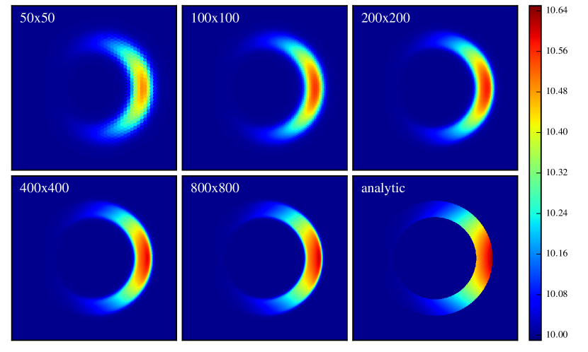
Figure 5: Anisotropic diffusion of a wedge along a circular magnetic field in 2D using full normal gradients and global timesteps. The panels show the CR energy density at time $t=10$ for different resolutions, as labelled, and the analytic solution for comparison. The minimum colormap is set to $9.98$ so that any values below the background value of $10$ would be clearly visible.

3 Test problems

To understand the accuracy and convergence properties of this scheme in its different variations we will discuss a set of idealized test problems. To construct a regular 2D mesh, we take a uniform Cartesian mesh and move the points in every second row by $0.45\,dx$ horizontally, where $dx$ is the cell size for the given resolution. Note that the resulting mesh is a regular hexagonal mesh, but its mesh-generating points are systematically offset from the centers of mass of the cells by about $1\%$ of the cell radius. We construct irregular meshes from these regular meshes by adding a random offset of up to $0.2\,dx$ in both dimensions, mimicking the typical deviation between mesh-generating points and cell centers in real problems (Vogelsberger et al., 2012). For all tests except the 2D blast wave (Sec. 3.5), we disable hydrodynamics and keep the mesh fixed. Note that the latter can amplify the overall error on irregular meshes, as the highly irregular cells stay as they are for the whole simulation time.

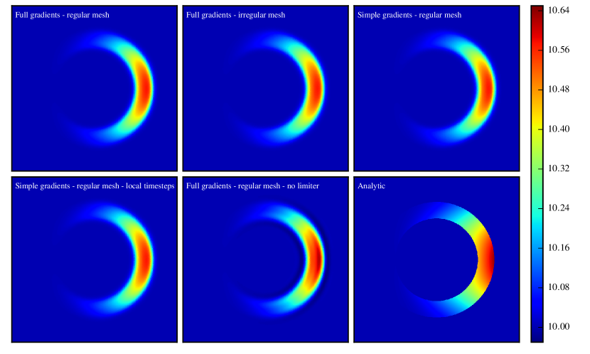
Figure 6: Anisotropic diffusion of a wedge along a circular magnetic field in 2D for a resolution of $200\times 200$ cells. The panels show the CR energy density at time $t=10$ for different methods, and the analytic solution for comparison.

3.1 Isotropic diffusion of a Gaussian profile

One of the most straightforward tests for isotropic diffusion is the evolution of a Gaussian profile over time. On a domain with extension $[-0.5,0.5]\times[-0.5,0.5]$, we set the CR energy density at the initial time $t_{0}=0.1$ to

$$\varepsilon_{\mathrm{cr}}\left(\textbf{{x}}\right)=1+\frac{10^{-2}}{2\pi D}\times e^{\frac{-r^{2}}{2D}},$$ (19)

where $r=\sqrt{\textbf{{x}}^{2}}$, $D=2\kappa_{\varepsilon}t$, and the diffusion coefficient is chosen as $\kappa=0.01$. We initialise all cells with the value of the CR energy density at their center of mass. We then advance the simulation from $t_{0}=0.1$ to $t=0.2$. At this time, the analytical solution is still given by Eq. (19). The $L^{1}$ norm measured for different resolutions on a regular and an irregular mesh is shown in Fig. 3. There is essentially no dependence of the accuracy of the solution on the structure of the mesh and the scheme always converges with second order.

3.2 Anisotropic diffusion of a wedge in a circular magnetic field

The anisotropic ring problem has become one of the standard test cases for anisotropic diffusion. We follow the setup of Parrish & Stone (2005) and Sharma & Hammett (2007). It sets the initial CR energy density on a domain of $[-1,1]^{2}$ to

$$\varepsilon_{\mathrm{cr}}\left(\textbf{{x}}\right)=\begin{cases}12&\mbox{if}\ 0.5<r<0.7\ \mathrm{and}\ \left|\phi\right|<\frac{\displaystyle\pi}{\displaystyle 12}\\ 10&\rm{else}.\end{cases}$$ (20)

Here, $r=\sqrt{\textbf{{x}}^{2}}$ is the radial coordinate and $\phi=\mathrm{atan2}\left(y,x\right)$ is the azimuthal coordinate. The magnetic field is given by

$$B_{x}\left(\textbf{{x}}\right) =-\frac{y}{r}$$ (21)

$$B_{y}\left(\textbf{{x}}\right) =+\frac{x}{r}.$$

Again, we initialise the cells with the values at their centers of mass, and use $\kappa=0.01$.

There are two regimes in which we can easily compute the analytical solution of the problem. At late times (we usually use $t=200$), diffusion in the azimuthal directions should have distributed the energy uniformly in the ring, so that $\varepsilon_{\mathrm{cr}}=10+1/6$ for $0.5<r<0.7$ and $\varepsilon_{\mathrm{cr}}=10$ everywhere else. The numerical solution at this time is sensitive to the amount of diffusion perpendicular to the magnetic field, but is insensitive to errors in the diffusion speed along magnetic field lines, as any information along the azimuth has been eliminated as a result of diffusion. Therefore, it is more demanding to compare the numerical solution to the analytical solution early on.

At early times (we use $t=10$ here), the energy that starts to diffuse from the initial wedge along magnetic field rings has not closed the ring yet. Therefore, we can at every radius treat the problem as a one-dimensional diffusion problem of a step function. The analytic solution is given by

$$\varepsilon_{\mathrm{cr}}\left(\textbf{{x}}\right)=10+\mathrm{erfc}\left[\left(\phi+\frac{\pi}{12}\right)\frac{r}{D}\right]-\mathrm{erfc}\left[\left(\phi-\frac{\pi}{12}\right)\frac{r}{D}\right],$$ (22)

with $D=\sqrt{4\kappa_{\varepsilon}t}$ for $0.5<r<0.7$ and $\varepsilon_{\mathrm{cr}}\left(\textbf{{x}}\right)=10$ everywhere else.

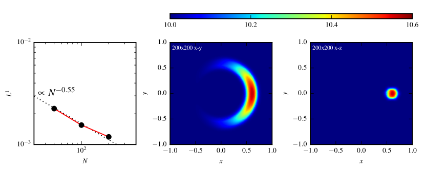
Figure 7: Anisotropic diffusion of a wedge along an azimuthal magnetic field in 3D. The left panel shows the $L^{1}$ norm at time $t=10$ for different resolutions. The center and right panels show slices of the CR energy density at $t=10$ in the $x-y$ and the $x-z$ plane, respectively.

The $L^{1}$ norms for different resolutions and different configurations of the anisotropic diffusion solver are shown in Fig. 4. The convergence rate at early times is identical for all four runs, independent of the regularity of the mesh, the use of simple or full normal gradient estimates, and the use of local or global timesteps. At late times, the only visible difference is that the error is larger for the run with local timesteps, but still converges at about the same rate as the other runs. The convergence rates at $t=10$ ($L^{1}\propto N^{-0.55}$) and $t=200$ ($L^{1}\propto N^{-0.7}$) are comparable to or slightly better than previous results (see, e.g. Parrish & Stone, 2005; Sharma & Hammett, 2007; Kannan et al., 2016). In all runs the minimum CR energy density is $10$, demonstrating that the limiting is sufficient to prevent violation of the entropy condition in this problem. Note also that the convergence rate at $t=200$ is significantly better than the convergence rate at $t=10$, because the errors of the diffusion problem along the magnetic field lines are eliminated because of the memory loss due to diffusion at $t=200$. Moreover, the convergence rate is significantly worse than first order ($L^{1}\propto N^{-1}$).

Therefore, computing a reference solution at higher resolution and comparing to this instead of the analytical solution (as done in Hopkins 2016) will significantly overestimate the convergence rate and is dangerous because it ultimately does not show that the scheme converges to the correct solution.

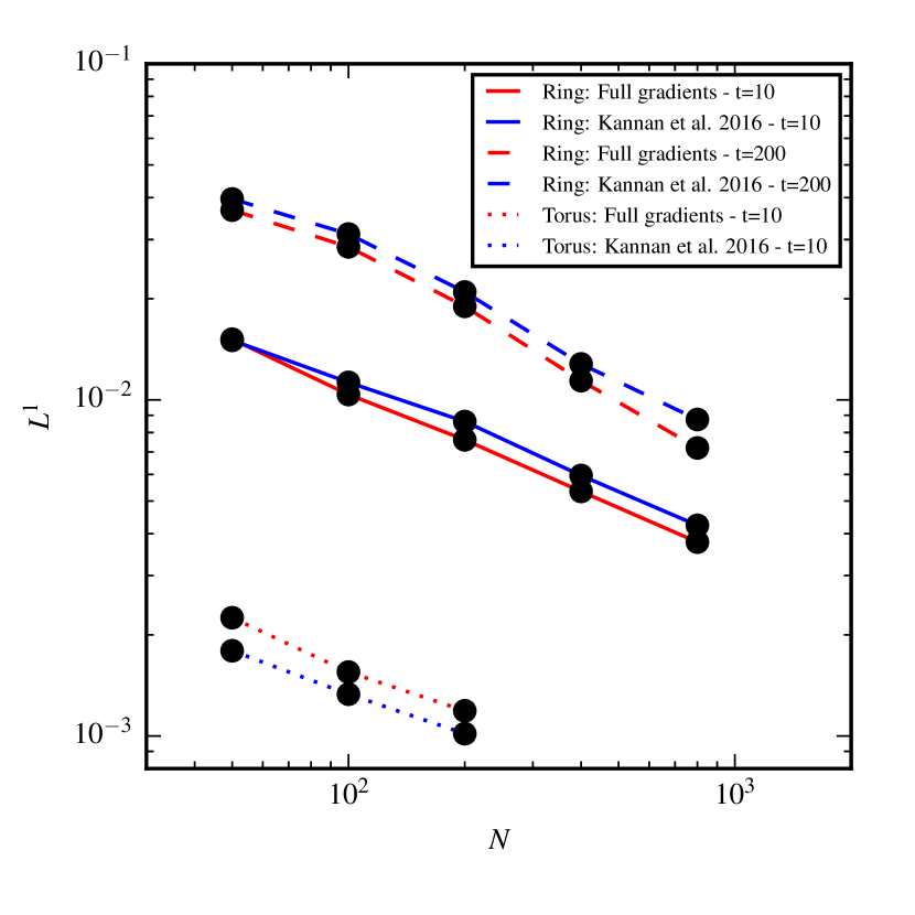
Figure 8: $L^{1}$ norm for anisotropic diffusion of an initial wedge in a circular magnetic field in 2D (ring) and 3D (torus). Solid and dashed lines show the $L^{1}$ norm for the 2D ring problem at $t=10$ and $t=200$, respectively. The dashed lines show the $L^{1}$ norm for the 3D torus problem at $t=10$. The red lines correspond to runs that use the full normal gradient estimate, the blue lines represent runs that use the implementation in Kannan et al. (2016). All runs use global timesteps.

Figure 5 shows the CR energy density for the run with full normal gradients and global timesteps on a regular mesh at $t=10$ for different resolutions. The main improvements with resolution are a reduction of diffusion in the radial direction and therefore a tighter ring, and a less peaked distribution of the CR energy density at the inner and outer boundaries of the ring. It can be nicely seen that there are no minima below the background CR energy density. Figure 6 shows the result at $t=10$ with a resolution of $200\times 200$ cells for different configurations of the anisotropic diffusion solver. As expected from the very similar $L^{1}$ norms, there is essentially no difference in the solutions. For the mesh setup we use here, there are no problematic corners for the full normal gradients. In general 3D simulations, the fraction of problematic corners can increase up to $20\%$. It is interesting to note that deactivating the limiter will lead to a measurable reduction of the order or a few percent of the CR energy density below the background value at the borders of the ring.

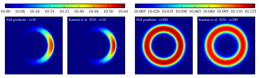
Figure 9: Anisotropic diffusion of an initial wedge in a circular magnetic field in 2D for a resolution of $200\times 200$ cells. The pair of panels on the left shows the CR energy density at $t=10$, the pair of panels on the right at $t=200$. The left panel of each pair shows a simulation that uses the full normal gradient estimate, the right panel of each pair shows a run that uses the implementation in Kannan et al. (2016). All simulations employ global timesteps.

Although we have shown that our scheme works well in 2D, a 3D test is also necessary, because the estimate of the gradient is significantly more complex in 3D. To this end, we generalise the anisotropic ring problem to 3D. Our initial wedge is now defined on the domain $[-0.5,0.5]^{3}$ by

$$\varepsilon_{\mathrm{cr}}\left(\textbf{{x}}\right)=\begin{cases}12&\!\!\mbox{if}\ \left[(0.6-r)^{2}+z^{2}-10^{-2}<0\right]\land\left(\left|\phi\right|<\frac{\pi}{12}\right),\\ 10&\!\!\rm{else}.\end{cases}$$ (23)

The $z$-component of the magnetic field is set to zero. The simulations are run on an irregular 3D mesh, starting from a hexagonal close-packed mesh and then randomly displacing mesh-generating points in the same way as done in 2D. The analytical solution at $t=10$ can again be computed by splitting the problem into 1D problems in azimuth.

The $L^{1}$ norm at $t=10$ and slices of the $x-y$ plane and the $x-z$ plane through the center are shown in Fig. 7. The convergence rate is essentially identical to the 2D problem. While the slice through the $x-y$ plane looks very similar to the 2D simulations, the slice through the $x-z$ plane shows that numerical diffusion in the radial and vertical directions is approximately of equal size.

3.3 Comparing the anisotropic diffusion solver with the method of Kannan et al. (2016)

While developing the scheme presented in this paper, our collaboration worked in parallel on a fundamentally different approach to anisotropic diffusion on unstructured meshes, which has recently been discussed in detail in Kannan et al. (2016). Here we briefly compare the two algorithms on the 2D ring and the 3D torus problems on a slightly disturbed mesh. The two main differences between the methods are that the scheme presented in Kannan et al. (2016) operates on the positions of the mesh-generating points in contrast to the scheme presented here that uses the centers of mass of the cells, and the size of the stencil needed differs when the time integration is generalised to individual timesteps.

In the scheme presented here, we need to include only the direct neighbours of active cells to compute the fluxes over all active interfaces which allows for the straightforward extension to local timesteps described above. In contrast, for the scheme presented in Kannan et al. (2016), we need to include a second layer of cells around active cells. However, this obviously does not make a difference for time integrations schemes that only work on global timesteps.

The $L^{1}$ norm at $t=10$ and $t=200$ for the 2D ring problem and the $L^{1}$ norm at $t=10$ for the 3D torus problem for both schemes are shown in Fig. 8. Both schemes converge essentially at the same rate, only the normalisation is slightly smaller in 2D and slightly larger in 3D for the method presented in this paper. The results for the 2D ring problem for the simulations with both schemes for a resolution of $200\times 200$ cells at $t=10$ and $t=200$ are shown in Fig. 9. While they are overall very similar, the errors in the two schemes are slightly different. At $t=10$, the maximum value is slightly lower in our scheme compared to the scheme presented in Kannan et al. (2016). At the same time, the solution for the method presented in Kannan et al. (2016) is more radially peaked towards the center of the ring. At $t=200$, the solutions are again very similar with a slightly higher peak value for the scheme presented here, which translates into a slightly smaller amount of numerical diffusion in the radial direction. We conclude that both schemes perform almost identically well and the differences are only in the details.

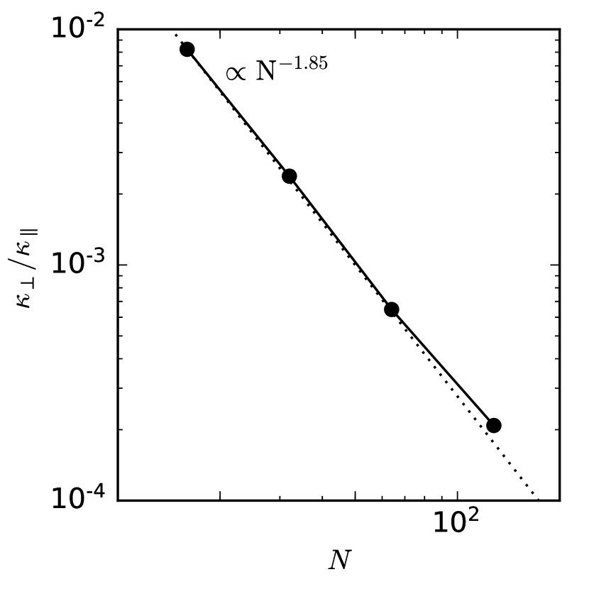
Figure 10: Ratio of the perpendicular numerical diffusion coefficient to the parallel diffusion coefficient for the Sovinec test problem as a function of resolution.

3.4 Measuring the perpendicular numerical diffusion coefficient with the Sovinec test

It is possible to directly measure the effective perpendicular diffusion coefficient that is entirely numerical in our simulations (Sovinec et al., 2004). We again use the same regular mesh we used for the 2D ring problem on a domain of $[-0.5,0.5]^{2}$, deactivate hydrodynamics, and keep the mesh fixed. We initialise the CR energy density with zero and the purely azimuthal magnetic field is given by

$$B_{x}\left(\textbf{{x}}\right) =+\cos{(x\pi)}\sin{(y\pi)},$$ (24)

$$B_{y}\left(\textbf{{x}}\right) =-\sin{(x\pi)}\cos{(y\pi)}.$$

CR energy is injected at a constant rate following the source term

$$\left.\frac{\partial\varepsilon_{\mathrm{cr}}\left(x,y\right)}{\partial t}\right|_{\mathrm{src}}=2\pi^{2}\cos{(x\pi)}\cos{(y\pi)}.$$ (25)

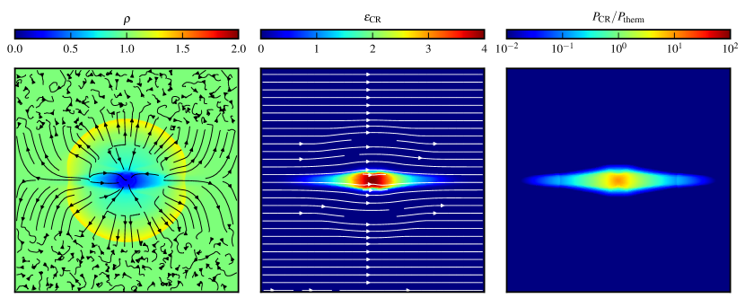
Figure 11: Slices of a 2D CR-driven blast wave with anisotropic CR diffusion. The left panel shows the gas density with velocity streamlines. The middle panel shows the CR energy density with magnetic field lines. The right panel shows the ratio between CR and thermal pressure. The simulation has been run with $512\times 512$ cells.

We employ a parallel diffusion coefficient of $\kappa_{\parallel}=1$ and a perpendicular diffusion coefficient of $\kappa_{\perp}=0$. We use outflow boundary conditions and fix the value of the CR energy density outside the computational domain to zero. Without numerical diffusion in the radial direction the CR energy in the computational domain should increase to infinity. However, because there is non-negligible numerical diffusion in the radial direction the CR energy density in the computational domain will eventually reach an equilibrium when the radial gradient is steep enough such that the radial diffusion out of the box balances the injection by the source term. Once equilibrium is reached, the effective numerical diffusion coefficient in the radial direction is directly given by the inverse of the CR energy density in the center of the computational domain (Sovinec et al., 2004),

$$\kappa_{\perp,\mathrm{num}}=\varepsilon_{\mathrm{cr}}\left(0,0\right)^{-1}.$$ (26)

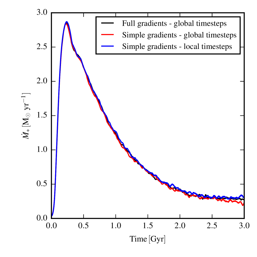
Figure 12: Time evolution of the star formation rate for the isolated disk for different configurations of the anisotropic diffusion solver.

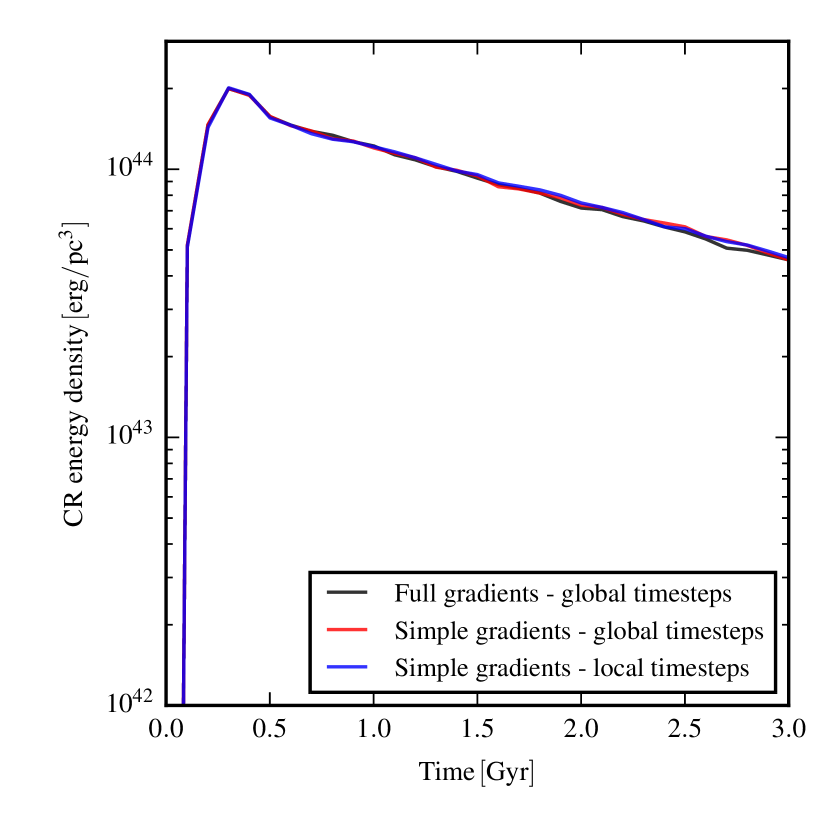
Figure 13: Time evolution of average CR energy density in a cylinder with a radius of $10$ kpc and a height of $1$ kpc, centered on the disk for different configurations of the anisotropic diffusion solver.

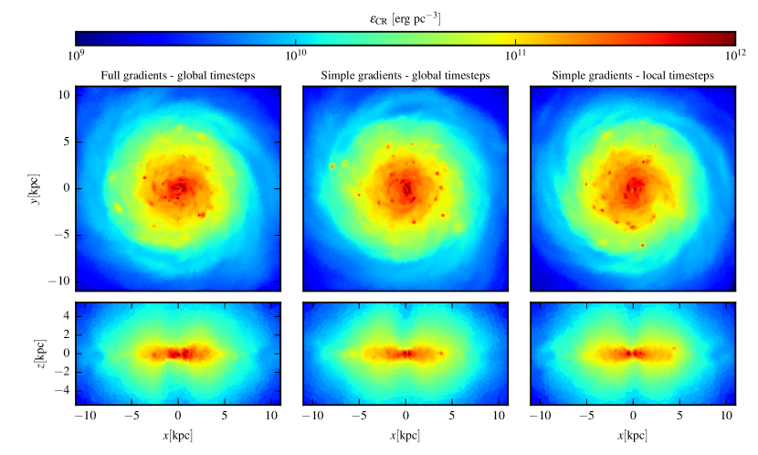
Figure 14: Slices of the CR energy density at time $t=1.5$ Gyrs. The columns show simulations with different configurations of the anisotropic diffusion solver. Top and bottom rows show face-on and edge-on slices through the center of the disk, respectively.

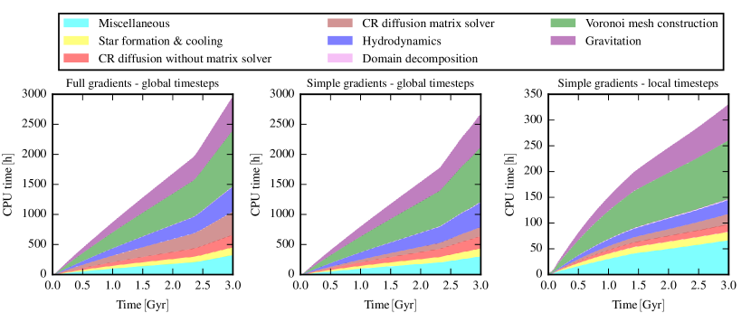
Figure 15: CPU time needed to run the isolated disk simulations to $t=3$ Gyrs for different configurations of the anisotropic diffusion solver. Note the different scale on the CPU time axis in the panel on the right-hand side.

The ratio $\kappa_{\perp,\mathrm{num}}/\kappa_{\parallel}$ for different resolutions is shown in Fig. 10. The effective perpendicular diffusion coefficient decreases almost with second order. Moreover, even for a resolution of only $16^{2}$ cells it is already smaller than $10^{-2}$ and decreases rapidly. This result is comparable or even slightly better than previous implementations of anisotropic diffusion (Parrish & Stone, 2005; Sharma & Hammett, 2007; Kannan et al., 2016). Therefore, we conclude that our implementation is able to guarantee a negligible amount of perpendicular numerical diffusion in practical problems.

3.5 2D blast wave with anisotropic diffusion

To test the anisotropic diffusion solver fully coupled with ideal MHD, we simulate a CR driven point explosion in 2D. We start with a regular mesh on a domain $[-0.5,0.5]^{2}$ with a homogeneous density of $\rho=1$, a homogeneous specific thermal energy of $u=2.5$, and a uniform magnetic field along the $x$-axis of $B_{x}=1$. We model the CRs with a constant $\gamma_{\mathrm{cr}}=4/3$ (Pfrommer et al., 2016) and set the initial CR energy to $\varepsilon_{\mathrm{cr}}=100$ for $r<0.02$ and to zero at larger radii. We set $\gamma_{\mathrm{gas}}=5/3$ and the kinetic energy-weighted anisotropic CR diffusion coefficient to $\kappa_{\varepsilon}=0.1$. We employ the new second order hydro scheme in arepo (Pakmor et al., 2016a) and use its standard ideal MHD implementation (Pakmor et al., 2011; Pakmor & Springel, 2013).

Figure 11 shows the simulation at $t=0.1$. The central injection of CR energy initially drives a spherical shock wave that is modified as CRs are able to escape along the magnetic field lines along the $x$-axis. There is no diffusion of CRs in the $y$-direction, therefore the shock wave in this direction behaves essentially like in a Sedov solution without diffusion. In particular, the gas in front of the shock is unperturbed. Close to the center the magnetic field lines are somewhat advected in the $y$-direction because of adiabatic expansion, but the $x$-component of the magnetic field still dominates. In contrast, CRs are able to diffuse freely in the $x$-direction, which leads to an enhancement of CRs ahead of the shock that already preconditions the velocity field ahead of the shock.

As in the pure diffusion test problems, there is essentially no diffusion of CRs perpendicular to the magnetic field lines, and the broadening of the CR energy density in the $y$-direction in the center is purely a result of advection due to adiabatic expansion.

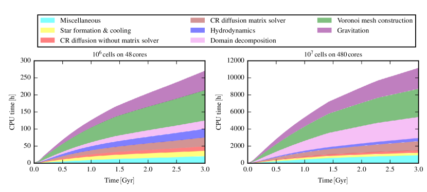
Figure 16: CPU time needed to run the isolated disk simulations to $t=3$ Gyrs for different resolutions and number of CPUs.

4 Anisotropic CR diffusion in isolated disk galaxies

One of the most interesting applications of anisotropic CR diffusion is the field of galaxy evolution, in particular as a driving mechanism for galactic winds (Uhlig et al., 2012; Booth et al., 2013; Salem & Bryan, 2014; Salem et al., 2014; Ruszkowski et al., 2016). Here we concentrate on testing our methodology by looking for differences caused by different configurations of the anisotropic diffusion solver in simulations of the formation and evolution of an isolated disk galaxy. For a detailed analysis of the physical implications of these simulations we refer to Pakmor et al. (2016b).

Our setup is close to one previously used in Pakmor & Springel (2013). A static background dark matter halo that follows a spherical NFW-profile (Navarro et al., 1996) with a concentration of $7.2$ and a total mass of $10^{11}\,\mathrm{M_{\odot}}$ is filled with gas in hydrostatic equilibrium (yielding a baryon fraction of $0.17$ in the halo) and made to rotate around the $z$-axis with a spin parameter of $\lambda=0.05$. We also add a uniform magnetic seed field along the $x$-axis with a strength of $10^{-10}\mathrm{G}$. We discretise the gas into $10^{6}$ cells of equal mass with a mass of $2\times 10^{4}\,\mathrm{M_{\odot}}$ and use the standard configuration for refinement and mesh regularization (Vogelsberger et al., 2012; Pakmor et al., 2016a). The interstellar medium is modelled by an effective equation of state (Springel & Hernquist, 2003). Star formation is handled probabilistically with a star formation rate that only depends on the local gas density (Springel & Hernquist, 2003).

We model the CRs in a two-fluid approximation with a constant adiabatic index of $4/3$ (Pfrommer et al., 2016). We initially set the CR energy density in all cells to zero, and whenever a star particle is created we inject $10^{48}$ erg of CR energy per solar mass of formed stars immediately into the neighbouring cells. We employ a kinetic energy-weighted diffusion coefficient for anisotropic CR diffusion of $\kappa_{\varepsilon}=10^{28}\mathrm{cm^{2}\,s^{-1}}$ and model CR cooling as described in Pfrommer et al. (2016).

In Figs. 12 and 13, we show the time evolution of the total star formation rate and the average CR energy density in a cylinder of radius $10$ kpc and height $1$ kpc centered on the disk, for different configurations of the anisotropic diffusion solver in otherwise identical runs. Both quantities are sensitive probes of the amount of CR diffusion out of the disk. Neither the change from the full normal gradient estimate to the simple normal gradient estimate, nor using local timesteps instead of global timesteps for the integration of the anisotropic diffusion problem have any impact on the results beyond the intrinsic noise induced by the probabilistic description of star formation.

This result is reinforced by Fig. 14, which shows slices of the CR energy density through the disk at $t=15$ Gyrs for three different configurations of the anisotropic diffusion solver. While there are differences in detail as the CR energy is injected in different places in the disk in the different runs, the overall CR energy distribution is very similar. The use of a constant diffusion coefficient quickly smoothes out any discontinuities in $\varepsilon_{\mathrm{cr}}$ as soon as anisotropic diffusion along the azimuthal magnetic field is efficient.

However, the different configurations of the anisotropic diffusion solver lead to very different runtimes for the same problem as shown in Fig. 15, even though the result is essentially identical as discussed above. In the most conservative configuration that employs global timesteps and the full normal gradient estimate, the CR diffusion solver takes about $20\%$ of the total runtime. Replacing the full normal gradient estimate with the simple normal gradient estimate reduces the fraction of the runtime used by the CR diffusion to about $13\%$. While these numbers clearly depend on the problem and more importantly on the resolution (the fraction of the total runtime used by the CR diffusion solver generally increases with resolution, as it scales worse than the gravity and hydrodynamics solvers), there is a significant speedup associated with using the simple normal gradient estimate.

A much larger speedup is achieved when changing from global to individual local timesteps, because the number of cells that requires a small timestep is often negligible compared to the total number of cells. As shown in Fig. 15, the total runtime drops by about a factor of $10$ while the fraction of the total runtime spent in the CR diffusion solver is only $10\%$. This clearly demonstrates again the importance of being able to use individual local timesteps to efficiently run simulations of galaxy formation. In fact, this is extremely critical for being able to simulate the formation and evolution of galaxies in the full cosmological framework at high resolution.

For all configurations, about half of the computational time of the diffusion problem is spent in the matrix solver. We expect this part of the calculation to be comparable in cost to similar solvers on Cartesian meshes (see, e.g. Parrish & Stone, 2005; Sharma & Hammett, 2007). The remaining parts of the diffusion solver are dominated by the computation of the coefficients for the gradient estimates and these calculations will be more expensive on our unstructured mesh. However, owing to the large speed-up obtained from using local timesteps, the diffusion solver only uses a small fraction of the overall runtime.

The weak scaling of the isolated galaxy simulation done with Arepo, including the semi-implicit diffusion solver, is explored in Fig. 16 with local timesteps and the full normal gradient estimate configuration for the diffusion solver. The run with $10^{7}$ cells requires about $40$ times more CPU time compared to the run with $10^{6}$ cells. The factor of $40$ is a result of a factor of $10$ for the increased number of resolution elements; a factor of $\sqrt[3]{10}\approx 2.2$ from the reduction in the timestep from smaller cell sizes; and a factor $\leq 2$ owing to the larger peak densities reached in the center of the galaxy. Interestingly, the CPU fraction spent in the diffusion solver is very similar for both runs, i.e. the weak scaling of the diffusion solver is comparable to the other parts of the code that dominate the runtime (gravity and mesh construction). The domain decomposition is the only part of the code that significantly increases its fraction of the total CPU time. However, this inefficiency could be alleviated by reducing the frequency of domain decompositions, which has not been attempted here. The good scaling of the diffusion solver suggests that it can be readily applied to large cosmological simulations in its current form.

5 Summary

We presented the formulation and implementation of a new numerical approach for treating the isotropic and anisotropic diffusion problem on unstructured, Voronoi meshes as used in the hydrodynamical AREPO code. The main features of our solver are:

• It is fully conservative.

• It does not violate the entropy condition $\Delta S>0$ in any significant way.

• It provides a semi-implicit time integration scheme with individual timesteps that only requires the solution of a single linear system of equations per timestep.

• Its convergence rate for isotropic diffusion is fully second order.

• For anisotropic diffusion, it has a comparable or slightly better convergence rate compared to previous implementations on structured and unstructured meshes.

The combination of these properties allows us to efficiently use the anisotropic diffusion solver in simulations of structure formation as well as galaxy formation and evolution without the need to make any compromises in terms of accuracy, conservation of energy, or violations of the entropy condition. The new method is thus enabling realistic treatments of cosmic ray physics in (computationally expensive) studies of galaxy formation, which is a particularly timely problem due to the relevance of cosmic rays for feedback processes. We demonstrate this in first science applications of our new methodology (Pakmor et al., 2016b; Simpson et al., 2016), and expect that our new approach will be very useful in future work that aims for a comprehensive modelling of galaxy formation physics.

References

- Blandford & Eichler (1987) Blandford R., Eichler D., 1987, Phys. Rep., 154, 1
- Booth et al. (2013) Booth C. M., Agertz O., Kravtsov A. V., Gnedin N. Y., 2013, ApJ, 777, L16
- Boulares & Cox (1990) Boulares A., Cox D. P., 1990, ApJ, 365, 544
- Brunetti & Lazarian (2007) Brunetti G., Lazarian A., 2007, MNRAS, 378, 245
- Chandran (2000) Chandran B. D. G., 2000, Physical Review Letters, 85, 4656
- Desiati & Zweibel (2014) Desiati P., Zweibel E. G., 2014, ApJ, 791, 51
- Dubois & Commerçon (2016) Dubois Y., Commerçon B., 2016, A&A, 585, A138
- Falgout & Yang (2002) Falgout R. D., Yang U. M., 2002, in Proceedings of the International Conference on Computational Science-Part III. ICCS ’02. Springer-Verlag, London, UK, UK, pp 632–641, http://dl.acm.org/citation.cfm?id=645459.653635
- Girichidis et al. (2016) Girichidis P., et al., 2016, ApJ, 816, L19
- Günter et al. (2005) Günter S., Yu Q., Krüger J., Lackner K., 2005, Journal of Computational Physics, 209, 354
- Hanasz et al. (2013) Hanasz M., Lesch H., Naab T., Gawryszczak A., Kowalik K., Wóltański D., 2013, ApJ, 777, L38
- Henson & Yang (2002) Henson V. E., Yang U. M., 2002, Applied Numerical Mathematics, 41, 155
- Hopkins (2016) Hopkins P. F., 2016, preprint, (arXiv:1602.07703)
- Kannan et al. (2016) Kannan R., Springel V., Pakmor R., Marinacci F., Vogelsberger M., 2016, MNRAS, 458, 410
- Kulsrud (2005) Kulsrud R. M., 2005, Plasma physics for astrophysics
- Kulsrud & Pearce (1969) Kulsrud R., Pearce W. P., 1969, ApJ, 156, 445
- Lerche (1967) Lerche I., 1967, ApJ, 147, 689
- Navarro et al. (1996) Navarro J. F., Frenk C. S., White S. D. M., 1996, ApJ, 462, 563
- Pakmor & Springel (2013) Pakmor R., Springel V., 2013, MNRAS, 432, 176
- Pakmor et al. (2011) Pakmor R., Bauer A., Springel V., 2011, MNRAS, 418, 1392
- Pakmor et al. (2016a) Pakmor R., Springel V., Bauer A., Mocz P., Munoz D. J., Ohlmann S. T., Schaal K., Zhu C., 2016a, MNRAS, 455, 1134
- Pakmor et al. (2016b) Pakmor R., Pfrommer C., Simpson C. M., Springel V., 2016b, ApJ, 824, L30
- Parrish & Stone (2005) Parrish I. J., Stone J. M., 2005, ApJ, 633, 334
- Pfrommer & Enßlin (2004) Pfrommer C., Enßlin T. A., 2004, A&A, 413, 17
- Pfrommer et al. (2016) Pfrommer C., Pakmor R., Schaal K., Simpson C. M., Springel V., 2016, preprint, (arXiv:1604.07399)
- Rodrigues et al. (2016) Rodrigues L. F. S., Sarson G. R., Shukurov A., Bushby P. J., Fletcher A., 2016, ApJ, 816, 2
- Ruszkowski et al. (2016) Ruszkowski M., Yang H.-Y. K., Zweibel E., 2016, preprint, (arXiv:1602.04856)
- Saad & Schultz (1986) Saad Y., Schultz M. H., 1986, SIAM Journal on Scientific and Statistical Computing, 7, 856
- Salem & Bryan (2014) Salem M., Bryan G. L., 2014, MNRAS, 437, 3312
- Salem et al. (2014) Salem M., Bryan G. L., Hummels C., 2014, ApJ, 797, L18
- Schlickeiser (2002) Schlickeiser R., 2002, Cosmic ray astrophysics. Springer., http://esoads.eso.org/cgi-bin/nph-bib_query?bibcode=2002cra..book.....S&db_key=AST
- Sharma & Hammett (2007) Sharma P., Hammett G. W., 2007, Journal of Computational Physics, 227, 123
- Sharma & Hammett (2011) Sharma P., Hammett G. W., 2011, Journal of Computational Physics, 230, 4899
- Simpson et al. (2016) Simpson C. M., Pakmor R., Marinacci F., Pfrommer C., Springel V., Glover S. C. O., Clark P. C., Smith R. J., 2016, preprint, (arXiv:1606.02324)
- Skilling (1971) Skilling J., 1971, ApJ, 170, 265
- Sovinec et al. (2004) Sovinec C. R., et al., 2004, Journal of Computational Physics, 195, 355
- Springel (2010) Springel V., 2010, MNRAS, 401, 791
- Springel & Hernquist (2003) Springel V., Hernquist L., 2003, MNRAS, 339, 289
- Tüllmann et al. (2000) Tüllmann R., Dettmar R.-J., Soida M., Urbanik M., Rossa J., 2000, A&A, 364, L36
- Uhlig et al. (2012) Uhlig M., Pfrommer C., Sharma M., Nath B. B., Enßlin T. A., Springel V., 2012, MNRAS, 423, 2374
- Vogelsberger et al. (2012) Vogelsberger M., Sijacki D., Kereš D., Springel V., Hernquist L., 2012, MNRAS, 425, 3024
- Wiener et al. (2013) Wiener J., Oh S. P., Guo F., 2013, MNRAS, 434, 2209
- Yan & Lazarian (2002) Yan H., Lazarian A., 2002, Physical Review Letters, 89, 1102
- Yan & Lazarian (2004) Yan H., Lazarian A., 2004, ApJ, 614, 757
- van Leer (1984) van Leer B., 1984, SIAM Journal on Scientific and Statistical Computing, 5, 1