CMB Lensing Bispectrum from Nonlinear Growth of the Large Scale Structure

Abstract

We discuss detectability of the nonlinear growth of the large-scale structure in the cosmic microwave background (CMB) lensing. The lensing signals involved in the CMB fluctuations have been measured from multiple CMB experiments, such as Atacama Cosmology Telescope (ACT), Planck, POLARBEAR, and South Pole Telescope (SPT). The reconstructed CMB lensing signals are useful to constrain cosmology via their angular power spectrum, while detectability and cosmological application of their bispectrum induced by the nonlinear evolution are not well studied. Extending the analytic estimate of the galaxy lensing bispectrum presented by Takada and Jain (2004) to the CMB case, we show that even near term CMB experiments such as Advanced ACT, Simons Array and SPT3G could detect the CMB lensing bispectrum induced by the nonlinear growth of the large-scale structure. In the case of the CMB Stage-IV, we find that the lensing bispectrum is detectable at $\gtrsim 50\sigma$ statistical significance. This precisely measured lensing bispectrum has rich cosmological information, and could be used to constrain cosmology, e.g., the sum of the neutrino masses and the dark-energy properties.

I Introduction

The cosmic microwave background (CMB) temperature and polarization anisotropies are distorted by gravitational weak lensing on arcminute scales. From the past several years, the lensing signals involved in observed CMB anisotropies have been detected from multiple CMB experiments, such as Atacama Cosmology Telescope (ACT) Das et al. (2011, 2014), Planck Planck Collaboration (2014); Planck Collaboration (2015a), POLARBEAR POLARBEAR Collaboration (2014), and South Pole Telescope (SPT) van Engelen et al. (2012); Story et al. (2015). The reconstructed lensing signals have also been used to cross-correlate with galaxies/quasars (e.g., Smith et al. (2007); Hirata et al. (2008); Bleem et al. (2012); Sherwin et al. (2012); Geach et al. (2013)) and cosmic infrared background (e.g., Planck Collaboration (2014); Holder et al. (2013); Hanson et al. (2013)).

Precisely measured lensing power spectra are already being used to constrain, e.g., the dark energy Sherwin et al. (2011); van Engelen et al. (2012); Planck Collaboration (2014), the sum of the neutrino masses Battye and Moss (2014), the non-Gaussianity of the primordial density perturbation Giannantonio and Percival (2014), a specific model of the cosmic string network Namikawa et al. (2013a), and a model of the dark-matter dark-energy interaction Wilkinson et al. (2014). Future CMB experiments are expected to quantify the sum of the neutrino masses (e.g., Namikawa et al. (2010); Abazajian et al. (2015); Wu et al. (2014); Allison et al. (2015) and references therein), and provide even tighter constraints on the dark energy, primordial non-Gaussianity, cosmic strings, and other fundamental physics. The ongoing and future CMB experiments such as Advanced ACT Calabrese et al. (2014), Simons Array Arnold et al. (2014), SPT3G Benson et al. (2014), and Stage-IV Abazajian et al. (2015) will significantly improve their sensitivity to CMB polarization at few arcminute scales, and realize very precise measurements of CMB lensing signals.

So far, multiple studies have focused on cosmological applications of reconstructed lensing signals using their angular power spectrum (two-point correlation). On the other hand, the possibility of detecting the bispectrum (three-point correlation) of the lensing signals has not been studied. In general, Gaussian fluctuations $\delta$ do not produce bispectrum, but fluctuations including the non-Gaussian part ($\delta+\delta^{2}+\cdots$) give rise to the nonzero bispectrum, such as $\langle\delta\delta\delta^{2}\rangle$ or $\langle\delta^{2}\delta^{2}\delta^{2}\rangle$. Since the nonlinear growth of the large-scale structure (LSS) produces the bispectrum of the lensing signals, measurements of the lensing bispectrum provide additional cosmological information involved in the nonlinear clustering. However, compared to other lensing measurements such as galaxy weak lensing, the nonlinear evolution of the density fluctuations does not significantly affect the lensing of the CMB. The effect of the nonlinear growth on the lensing power spectrum is only important at $\ell\gtrsim 1000$ Lewis and Challinor (2006). The weakness of the nonlinear effect comes from the fact that the gravitational potential which causes the CMB lensing is at relatively high-redshifts ($z\sim\mathcal{O}(1)$) Lewis and Challinor (2006) where the gravitational potential would be described with linear perturbation theory at even small scales. In addition, the lensing potential is a line-of-sight integral over the dark matter structures, and is a sum of the gravitational potential at different redshifts. This summation along the line-of-sight Gaussianizes the lensing potential by the central limit theorem Hirata and Seljak (2003a), and the lensing bispectrum becomes small.

In past and ongoing CMB experiments which cannot extract small-scale lensing signals, the nonlinear effect does not significantly bias the cosmological parameter estimations. However, future CMB experiments such as CMB Stage-IV (S4) will realize very deep polarization measurement up to few arcminute scales, and precision of the lensing reconstruction will be improved significantly. In upcoming and future CMB experiments, the nonlinear growth of the LSS will be no longer negligible in the CMB analysis, and cause bias in several ways. Challinor and Lewis Challinor and Lewis (2005) showed that B-mode polarization generated by lensing has $\sim 10$% of the nonlinear contributions even at large scale $\ell<100$. Boehm et al. Boehm et al. (2016) discuss how the presence of the lensing bispectrum biases the lensing reconstruction in S4, finding that there is a non-negligible contribution from the bispectrum in the power spectrum estimate.

In this paper, we consider for the first time the nonlinear effect as a cosmological signal rather than a source of the bias, and discuss the detectability and cosmological application of the lensing bispectrum in CMB Stage-III (S3) and S4 experiments. We extend Takada and Jain (2004) Takada and Jain (2004) (hereafter TJ04) to the case with the CMB lensing to compute the lensing bispectrum and its signal to noise. We then discuss the cosmological application of the lensing bispectrum.

This paper is organized as follows. In Sec. II, we summarize our analytic method to compute the lensing bispectrum. In Sec. III, we show the expected signal to noise of the lensing bispectrum from near term and future CMB experiments. We also show the impact of the inclusion of the lensing bispectrum in the cosmological parameter constraints. Section IV is devoted to a summary.

Throughout this paper, for the fiducial model, we assume the spatially flat $\Lambda$CDM cosmology with two massive ($m_{\nu,1}=0.05$ eV and $m_{\nu,2}=0.01$ eV mass eigenstates) and one massless neutrinos. We use a set of cosmological parameters consistent with the latest Planck results Planck Collaboration (2015b); the baryon and matter density, $\Omega_{\rm b}h^{2}=0.0223$ and $\Omega_{\rm m}h^{2}=0.119$, the dark-energy density $\Omega_{\Lambda}=0.689$, the amplitude of the primordial scalar power spectrum, $A_{\rm s}=2.13\times 10^{-9}$, and its spectral index at $k=0.05$ Mpc^-1, $n_{\rm s}=0.965$, and the reionization optical depth $\tau=0.0630$. We employ CAMB Lewis et al. (2000) to compute the linear matter power spectrum at $z=0$ and lensing power spectrum. The linear matter power spectrum at $z=0$ is then used to evaluate those at each redshift $z$. We employ the fitting formula given by Refs. Smith et al. (2003); Takahashi et al. (2012) to compute the nonlinear matter power spectrum from the linear matter power spectrum.

II CMB Lensing Bispectrum

Here we summarize the bispectrum of the CMB lensing signals. Our method to compute the CMB lensing bispectrum is based on TJ04.

The distortion effect of lensing on the primary CMB anisotropies is expressed by a remapping (e.g. Lewis and Challinor (2006)). This introduces statistical anisotropy into the observed CMB, in the form of a correlation between the CMB anisotropies and their gradient Hu and Okamoto (2002). With a large number of observed CMB modes, this correlation is used to estimate the lensing signals involved in observed CMB anisotropies Zaldarriaga and Seljak (1999); Hu and Okamoto (2002); Hirata and Seljak (2003b); Hanson and Lewis (2009). The power spectrum of the lensing signals is in turn studied by taking the power spectrum of these lensing estimates Hu and Okamoto (2002); Namikawa et al. (2013b).

The reconstructed lensing signals are also used to study other statistics such as the bispectrum. The bispectrum of the CMB lensing-mass (convergence) fields is defined as

$$\langle\kappa_{\ell_{1}m_{1}}\kappa_{\ell_{2}m_{2}}\kappa_{\ell_{3}m_{3}}\rangle=\begin{pmatrix}\ell_{1}&\ell_{2}&\ell_{3}\\ m_{1}&m_{2}&m_{3}\end{pmatrix}B^{\kappa}_{\ell_{1}\ell_{2}\ell_{3}}\,,$$ (1)

where $\kappa_{\ell m}$ is the spherical harmonic coefficients of the lensing-mass fields, and $\langle\cdots\rangle$ denotes the ensemble average. The multipoles satisfy the triangle condition, $|\ell_{i}-\ell_{j}|\leq\ell_{k}\leq\ell_{i}+\ell_{j}$.

Note that, in the flat sky, with the Dirac delta function $\delta_{\rm D}$, the bispectrum is given by

$$\langle\kappa_{\bm{\ell}_{1}}\kappa_{\bm{\ell}_{2}}\kappa_{\bm{\ell}_{3}}\rangle=(2\pi)^{2}\delta_{\rm D}(\bm{\ell}_{1}+\bm{\ell}_{2}+\bm{\ell}_{3})B^{\kappa}(\bm{\ell}_{1},\bm{\ell}_{2},\bm{\ell}_{3})\,,$$ (2)

where $\kappa_{\bm{\ell}}$ is the two-dimensional Fourier mode of the lensing-mass fields. The full-sky bispectrum is then approximately related to the flat-sky bispectrum as Takada and Jain (2004)

$$B^{\kappa}_{\ell_{1}\ell_{2}\ell_{3}}\simeq\begin{pmatrix}\ell_{1}&\ell_{2}&\ell_{3}\\ 0&0&0\end{pmatrix}$$

$$\qquad\times\sqrt{\frac{(2\ell_{1}+1)(2\ell_{2}+1)(2\ell_{3}+1)}{4\pi}}B^{\kappa}(\bm{\ell}_{1},\bm{\ell}_{2},\bm{\ell}_{3})\,.$$ (3)

Denoting $L=(\ell_{1}+\ell_{2}+\ell_{3})/2$, an approximate form of the Wigner 3j symbol is given by Takada and Jain (2004)

$$\begin{pmatrix}\ell_{1}&\ell_{2}&\ell_{3}\\ 0&0&0\end{pmatrix}\simeq(-1)^{L}\sqrt{\frac{\hskip 1.00006pt{\rm e}}{2\pi}}(L+1)^{-1/4}$$

$$\qquad\times\prod_{i=1}^{3}(L-\ell_{i}+1)^{-1/4}\left(\frac{L-\ell_{i}+1/2}{L-\ell_{i}+1}\right)^{L-\ell_{i}+1/4}\,.$$ (4)

In our calculation, we evaluate the full-sky bispectrum from the flat-sky bispectrum given by Eqs. (3) and (4).

The lensing-mass field is the line-of-sight integral over the gravitational potential of the LSS, and is directly related to the matter inhomogeneities. The flat-sky lensing bispectrum is expressed in terms of the three-dimensional matter bispectrum as

$$B^{\kappa}(\bm{\ell}_{1},\bm{\ell}_{2},\bm{\ell}_{3})={\int_{0}^{\chi_{*}}\!\!\,{\rm d}\chi\,\,}\frac{W^{3}(\chi)}{\chi^{4}}B^{\rm m}(\bm{k}_{1},\bm{k}_{2},\bm{k}_{3},\chi)\,,$$ (5)

where $\bm{k}_{i}=\bm{\ell}_{i}/\chi$, and the lensing kernel is given by

$$W(\chi)=\frac{3\Omega_{\rm m,0}H_{0}^{2}}{2a(\chi)}\frac{\chi(\chi_{*}-\chi)}{\chi_{*}}\,.$$ (6)

The quantities, $\chi$, $\Omega_{\rm m,0}$, $a$, and $H_{0}$, denote the comoving distance, matter energy density, scale factor, and current expansion rate of the Universe. $\chi^{*}$ is the comoving distance to the last scattering surface of CMB photons. Compared to the galaxy lensing, the above lensing kernel is sensitive to the structure at relatively high redshifts [$z\sim\mathcal{O}(1)$] Lewis and Challinor (2006). In addition, since $\ell=k\chi$, for a given multipole $\ell$, CMB lensing signals pick up the density fluctuations at larger scales compared to the galaxy lensing. The lensing signals are therefore less sensitive to the nonlinear growth of the LSS at the late time of the Universe.

The matter bispectrum is induced by the nonlinear clustering in the matter density fluctuations. The thorough calculation of the nonlinear clustering, however, requires an expensive numerical simulations. To clarify the feasibility of the lensing bispectrum in cosmology, TJ04 computed the matter bispectrum using a fitting formula for the matter bispectrum. We follow TJ04 and use the best available fitting formula for the matter bispectrum which is recently developed by Ref. Gil-Marin et al. (2012) and is an extension of the formula in Ref. Scoccimarro and Couchman (2001). In this formula, the matter bispectrum is given by

$$B^{\rm m}(\bm{k}_{1},\bm{k}_{2},\bm{k}_{3},\chi) =2F_{2}(\bm{k}_{1},\bm{k}_{2},z)P_{\rm m}(k_{1},z)P_{\rm m}(k_{2},z)$$

$$+2\,{\rm perms.}\,,$$ (7)

where $P_{\rm m}(k,z)$ is the nonlinear matter power spectrum and, with $\bm{k}_{1}\cdot\bm{k}_{2}=k_{1}k_{2}\cos\theta$, the “effective” F2 kernel is defined as Scoccimarro and Couchman (2001)

$$F_{2}(\bm{k}_{1},\bm{k}_{2},z)=\frac{5}{7}a(k_{1},z)a(k_{2},z)$$

$$\qquad+\frac{k_{1}^{2}+k_{2}^{2}}{2k_{1}k_{2}}b(k_{1},z)b(k_{2},z)\cos\theta$$

$$\qquad+\frac{2}{7}c(k_{1},z)c(k_{2},z)\cos^{2}\theta\,.$$ (8)

The factors $a(k,z)$, $b(k,z)$ and $c(k,z)$ are defined by Scoccimarro and Couchman (2001)

$$a(k,z) =\frac{1+\sigma_{8}^{a_{6}}(z)\sqrt{0.7Q(n_{\rm eff})}(qa_{1})^{n_{\rm eff}+a_{2}}}{1+(qa_{1})^{n_{\rm eff}+a_{2}}}$$ (9)

$$b(k,z) =\frac{1+0.2a_{3}(n_{\rm eff}+3)(qa_{7})^{n_{\rm eff}+3+a_{8}}}{1+(qa_{7})^{n_{\rm eff}+3.5+a_{8}}}$$ (10)

$$c(k,z) =\frac{1+[4.5a_{4}/(1.5+(n_{\rm eff}+3)^{4})](qa_{5})^{n_{\rm eff}+3+a_{9}}}{1+(qa_{5})^{n_{\rm eff}+3.5+a_{9}}}\,,$$ (11)

with $Q(x)=(4-2^{x})/(1+2^{x+1})$. The quantity, $\sigma_{8}(z)$ is the variance of the matter density fluctuations smoothed by $8$Mpc $h^{-1}$ at redshift $z$. $n_{\rm eff}\equiv d\ln P_{\rm m}^{\rm lin}(k)/dk$ is the effective spectral index of the power spectrum, with $P_{\rm m}^{\rm lin}(k)$ being the linear matter power spectrum. We define $q=k/k_{\rm NL}$ with the nonlinear scale $k_{\rm NL}$ satisfying $4\pi k^{3}_{\rm NL}P_{\rm m}^{\rm lin}(k_{\rm NL})=1$. The coefficients of the fitting formula $a_{i}$ ($i=1,2,\dots,9$) are obtained by fitting to the simulations in Ref. Gil-Marin et al. (2012), and their best fit parameters are $a_{1}=0.484$, $a_{2}=3.740$, $a_{3}=-0.849$, $a_{4}=0.392$, $a_{5}=1.013$, $a_{6}=-0.575$, $a_{7}=0.128$, $a_{8}=-0.722$, and $a_{9}=-0.926$.

At $k\ll k_{\rm NL}$ ($q\ll 1$), the effective F2 kernel recovers the second order (tree-level) prediction of Eulerian perturbation theory in an Einstein de-Sitter universe. The tree-level bispectrum is computed with $P_{\rm m}^{\rm lin}$ in Eq. (7), and $a=b=c=1$ in Eq. (8).

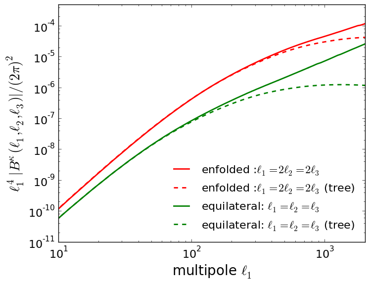
Figure 1: The lensing bispectra with the enfolded ($\ell_{1}=2\ell_{2}=2\ell_{3}$; red) and equilateral ($\ell_{1}=\ell_{2}=\ell_{3}$; green) triangular configurations in the multipole space. The dashed lines (denoted by “tree”) show the bispectrum from the tree-level prediction.

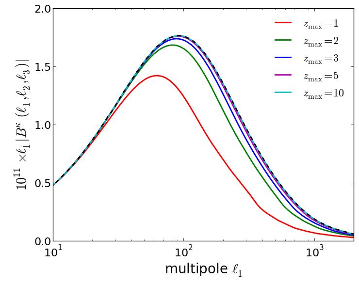
Figure 2: The contribution to the enfolded ($\ell_{1}=2\ell_{2}=2\ell_{3}$) lensing bispectrum from the gravitational potential of the LSS between $z=0$ and $z_{\rm max}$. The black dashed line shows the full lensing bispectrum. The maximum redshift is varied from $z_{\rm max}=1$ to $10$. For illustrative purposes, we multiply $10^{11}\ell_{1}$ to the lensing bispectrum.

Figure 1 shows the CMB lensing bispectrum computed from Eq. (5). We show the following two cases: the enfolded ($\ell_{1}=2\ell_{2}=2\ell_{3}$) and, for comparison with TJ04, the equilateral ($\ell_{1}=\ell_{2}=\ell_{3}$) triangular configurations. We also plot the bispectra from the tree level prediction. As we discussed later, the enfolded bispectrum provides the most part of the signal to noise. The tree-level bispectrum starts to deviate from the full nonlinear bispectrum at $\ell\sim\mathcal{O}(100)$. The enfolded bispectrum has no significant corrections from the full nonlinear effect even at $\ell\sim 1000$. On the other hand, in the case of the galaxy weak lensing, the full nonlinear contribution is important even at large scales $\ell\sim\mathcal{O}(10)$ Takada and Jain (2004), and the tree-level contribution is several orders of magnitude smaller than the full nonlinear contribution at $\ell=1000$. This fact indicates that, compared to the galaxy lensing bispectrum, the CMB lensing bispectrum is much less sensitive to the nonlinear clustering beyond the tree level. Note that the amplitude of the enfolded bispectrum is larger than that of the equilateral bispectrum. This is because the matter bispectrum at smaller scales (equivalent to low redshifts for a given multipole) which produces most of the lensing signals has large amplitudes in the enfolded configuration Jeong and Komatsu (2009); Schmittfull et al. (2013).

Figure 2 shows the contributions from $z=0$ to $z_{\rm max}$ to the enfolded lensing bispectrum. The lensing bispectrum is mostly generated from lower redshifts $z\leq 3$. The contributions from higher redshifts $z\geq 5$ are negligible in the lensing bispectrum. We also check that the equilateral case has also similar $z_{\rm max}$ dependence.

III Cosmological Forecasts

We next show the expected signal to noise of the lensing bispectrum from the near future CMB experiments.

III.1 Detectability of the lensing bispectrum

Table 1: Experimental specifications for CMB experiments considered in this paper: the noise level in the polarization map ($\Delta_{\rm P}$) in unit of $\mu$K-arcmin, the beam size of FWHM ($\theta$) in unit of arcmin, and fractional sky coverage $f_{\rm sky}$.

	$\Delta_{\rm P}$ [$\mu$K-arcmin]	$\theta$ [arcmin]	$f_{\rm sky}$
S3-wide	6	1	0.5
S3-deep	3	1	0.05
S4	1	3	0.5

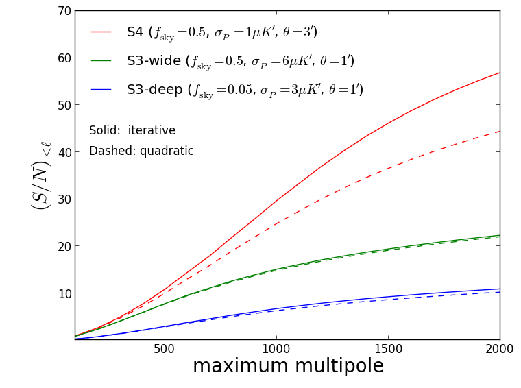
Figure 3: Expected cumulative signal to noise ratios of the CMB lensing bispectrum with the S3-wide (such as Advanced ACT and Simons Array), the S3-deep (such as SPT3G) and the CMB Stage-IV. The dashed lines show the cases with the noise spectra computed from the quadratic estimator of Ref. Hu and Okamoto (2002).

We estimate the detectability of the lensing bispectrum as Takada and Jain (2004)

$$\left(\frac{S}{N}\right)^{2}_{\leq\ell} =f_{\rm sky}\sum^{\ell}_{\ell_{1}\leq\ell_{2}\leq\ell_{3}}\frac{(B^{\kappa}_{\ell_{1}\ell_{2}\ell_{3}})^{2}}{\Delta_{\ell_{1}\ell_{2}\ell_{3}}\mathcal{C}_{\ell_{1}}\mathcal{C}_{\ell_{2}}\mathcal{C}_{\ell_{3}}}\,,$$ (12)

where $\mathcal{C}_{\ell}$ is the sum of the signal and noise power spectrum in the CMB lensing reconstruction. We define $\Delta_{\ell_{1}\ell_{2}\ell_{3}}=1$ if all $\ell_{i}$ are different, $\Delta_{\ell_{1}\ell_{2}\ell_{3}}=2$ if two of $\ell_{i}$ are equal, and $\Delta_{\ell_{1}\ell_{2}\ell_{3}}=6$ if all of $\ell_{i}$ are equal, respectively. The Gaussian covariance of the lensing bispectrum is assumed in the above equation. The noise power spectrum of the lensing signals, $N^{\phi}_{\ell}$, is computed based on the iterative estimator developed in Refs. Hirata and Seljak (2003a); Smith et al. (2012).

To compute the noise power spectrum of the lensing signals, $N^{\phi}_{\ell}$, in Eq. (12), we assume a white noise with a Gaussian beam. We employ the formula of the noise power spectrum in Ref. Knox (1999) which is characterized by the following two parameters; the noise level $\Delta_{\rm P}$ in unit of $\mu$K-arcmin, and beam size of FWHM $\theta$ in unit of arcmin. The summary of the experimental specifications are given in Table. 1. We denote “S3-wide” as a wide Stage-III class experiment such as Advanced ACT and Simons Array, and “S3-deep” as a deep Stage-III class experiment such as SPT3G. We choose $\Delta_{\rm P}=6\mu$K-arcmin and $\theta=1$ arcmin for the S3-wide, $\Delta_{\rm P}=3\mu$K-arcmin and $\theta=1$ arcmin for the S3-deep, and $\Delta_{\rm P}=1\mu$K-arcmin and $\theta=3$ arcmin or the S4. For the S3-wide and S4 experiments, we assume the fractional survey area as $f_{\rm sky}=0.5$, while we choose $f_{\rm sky}=0.05$ for S3-deep. The CMB multipoles up to $\ell=4000$ are used to estimate the noise power spectrum.

Figure 3 shows the signal-to-noise ratio of the S3-wide, S3-deep and S4 experiments. Even the Stage-III experiments would detect the CMB lensing bispectrum. In the case of S4, the lensing bispectrum will be detected with high statistical significance ($\gtrsim 50\sigma$). Note that, for S3-wide and S3-deep, the signal-to-noise ratio is almost unchanged even if we use the quadratic estimator developed in Ref. Hu and Okamoto (2002). On the other hand, the signal-to-noise ratio with the quadratic estimator decreases by $\sim 20$% for the S4 experiment.

We check that the most dominant contribution to the signal-to-noise ratio comes from the enfolded bispectrum. As shown in Fig. 1, the tree-level terms significantly contribute to the enfolded configuration even at $\ell\sim 2000$. This fact indicates that terms beyond the tree level are not so significant unless we include the lensing signals only at $\ell\lesssim 2000$.

III.2 Cosmological Parameter Constraints

Table 2: Expected $1\sigma$ constraints on the beyond-$\Lambda$CDM parameters (the dark-energy equation-of-state $w$ and the sum of neutrino masses $\sum m_{\nu}$), using the lensing power spectrum (2pt), the lensing bispectrum (3pt), and both the lensing power spectrum and bispectrum (2pt+3pt). The prior information from the primary CMB anisotropies is included in all cases. The noise spectra are computed assuming the CMB Stage-IV. We also show the improvements by adding the lensing bispectrum to the lensing power spectrum.

	2pt	3pt	2pt+3pt	Improvement (%)
$w$	0.16	0.21	0.12	33%
$\sum m_{\nu}$ [meV]	74	68	55	35%

A precisely measured bispectrum would be useful to explore various issues in cosmology. As an example of cosmological applications, we here discuss improvement on cosmological parameter constraints if the lensing bispectrum is further included in the analysis.

We compute expected constraints on cosmological parameters based on the Fisher matrix approach. Following TJ04, the Fisher information matrix of the lensing bispectrum is given by Takada and Jain (2004)

$$F_{ij}=f_{\rm sky}\sum_{\ell_{1}\leq\ell_{2}\leq\ell_{3}}\frac{B^{\kappa}_{\ell_{1}\ell_{2}\ell_{3},i}B^{\kappa}_{\ell_{1}\ell_{2}\ell_{3},j}}{\Delta_{\ell_{1}\ell_{2}\ell_{3}}\mathcal{C}_{\ell_{1}}\mathcal{C}_{\ell_{2}}\mathcal{C}_{\ell_{3}}}\,,$$ (13)

where $B^{\kappa}_{\ell_{1}\ell_{2}\ell_{3},i}$ is the derivative of the lensing bispectrum with respect to the $i$th cosmological parameter. We choose the maximum multipole of the summation of Eq. (13) as $\ell=2000$. In addition to the Fisher matrix of the lensing bispectrum, the Fisher matrix from the primary CMB anisotropies and lensing power spectrum is added in our analysis, and we ignore the cross covariance between the power spectrum and bispectrum of the lensing signals. We marginalize the six $\Lambda$CDM cosmological parameters ($\ln\Omega_{\rm b}h^{2}$, $\ln\Omega_{\rm m}h^{2}$, $\Omega_{\Lambda}$, $\ln A_{\rm s}$, $n_{\rm s}$, $\tau$), the dark-energy equation-of-state $w$, and the sum of the neutrino masses $\sum m_{\nu}$. The instrumental noise power spectrum is computed assuming S4. The derivatives are computed based on the symmetric difference quotient.

Table 2 shows the expected $1\sigma$ constraints on $w$ and $\sum m_{\nu}$ using the lensing power spectrum (2pt), the lensing bispectrum (3pt), and both the lensing power spectrum and bispectrum (2pt+3pt). In all cases, we compute the Fisher matrix by adding the prior information matrix from the CMB temperature and E-mode polarization following e.g. Eqs. (4.4) and (4.5) of Hannestad et al. (2006). Note that the constraints from the lensing power spectrum are consistent with other previous works Allison et al. (2015); Wu et al. (2014) but for a different scenario of the massive neutrinos. Comparing with the constraints from the lensing power spectrum (2pt), the inclusion of the lensing bispectrum (2pt+3pt) improves the constraint on the dark-energy equation-of-state $w$ and the sum of neutrino masses $\sum m_{\nu}$ by $33$% and $35$%, respectively. We find that the constraints on $w$ and $\sum m_{\nu}$ from the lensing bispectrum (3pt) are comparable to those from the lensing power spectrum (2pt). Note that the dark-energy density, $\Omega_{\Lambda}$, is also improved by $\sim 20$%. These results indicate that the lensing bispectrum measured by the S4 experiment could provide additional information on the dark energy and the neutrino masses, and also be used for other cosmological purposes.

IV Summary

We discussed the detectability of the CMB lensing bispectrum and its cosmological application in the near future CMB experiments such as Advanced ACT, Simons Array, SPT3G, and S4. We found that the lensing bispectrum is detectable even from the near term CMB experiments. In the case of S4, the lensing bispectrum would be detected with high statistical significance ($\gtrsim 50\sigma$). We then showed that the inclusion of the lensing bispectrum measurement further improves the constraints on the dark-energy parameters ($w$ and $\Omega_{\Lambda}$) and the sum of neutrino masses.

We have focused on the lensing bispectrum obtained from the CMB experiments. The cross bispectrum between other cosmological observables such as the galaxy clustering, cosmic shear, and cosmic infrared background may be also detectable in ongoing and future experiments, and is important to be investigated.

We have made several simple assumptions in our estimation to compute analytically. Although we assume the Gaussian covariance of the bispectrum to estimate the signal to noise, the non-Gaussian covariance may degrade the sensitivity to the lensing bispectrum, and therefore cosmology Sefusatti et al. (2006). In the Fisher matrix, we also ignored the cross covariance between the power spectrum and bispectrum which comes from the non-Gaussianity of the lensing signals and could degrade the cosmological constraints. From these respects, the expected signal to noise and constraints obtained in this paper are considered as their upper limits, though the non-Gaussianity of the lensing signals is expected to be much less significant compared to the case with the galaxy lensing shown in TJ04. The precision of the fitting formula Gil-Marin et al. (2012) could also affect the resultant signal to noise ratio and parameter constraints. The fitting formula should be therefore tested against a wide range of cosmological parameters for a robust forecast and a realistic cosmological analysis. Even in the absence of the nonlinear gravitational potential, the post-Born correction generates a bispectrum in the observed lensing signals, and could bias in estimating the nonlinear growth Pratten and Lewis (2016). The validity of our assumptions is worth investigating, and will be addressed in our future work. Albeit simple, our results definitely show that the nonlinear evolution will be no longer negligible in ongoing and near future CMB experiments, and will have fruitful cosmological information comparable to that from the lensing power spectrum.

At the time of writing this paper, Boehm et al. Boehm et al. (2016) explore the bias in the lensing reconstruction induced by the lensing bispectrum, finding that there is an additional non-negligible bias in estimating the lensing power spectrum in the case of S4. Their result also implies that, in the era of S4, the effect of the nonlinear growth should be properly taken into account even in the CMB lensing analysis.