Axial compression of a thin elastic cylinder: bounds on the minimum energy scaling law

Abstract.

We consider the axial compression of a thin elastic cylinder placed about a hard cylindrical core. Treating the core as an obstacle, we prove upper and lower bounds on the minimum energy of the cylinder that depend on its relative thickness and the magnitude of axial compression. We focus exclusively on the setting where the radius of the core is greater than or equal to the natural radius of the cylinder. We consider two cases: the “large mandrel” case, where the radius of the core exceeds that of the cylinder, and the “neutral mandrel” case, where the radii of the core and cylinder are the same. In the large mandrel case, our upper and lower bounds match in their scaling with respect to thickness, compression, and the magnitude of pre-strain induced by the core. We construct three types of axisymmetric wrinkling patterns whose energy scales as the minimum in different parameter regimes, corresponding to the presence of many wrinkles, few wrinkles, or no wrinkles at all. In the neutral mandrel case, our upper and lower bounds match in a certain regime in which the compression is small as compared to the thickness; in this regime, the minimum energy scales as that of the unbuckled configuration. We achieve these results for both the von Kármán-Donnell model and a geometrically nonlinear model of elasticity.

1. Introduction

In many controlled experiments involving the axial compression of thin elastic cylinders, one observes complex folding patterns (see, e.g., [9, 15, 23, 25]). It is natural to wonder if such patterns are required to minimize elastic energy, or if they are instead due to loading history. Before we can begin to answer these questions, we need to understand the minimum energy and in particular its dependence on external parameters. This paper offers progress towards this goal.

Since the work of Horton and Durham [15], it is a common experimental practice to place the elastic cylinder about a hard inner core that stabilizes its deformation during loading. In this paper, we consider the minimum energy of a compressed thin elastic cylinder fit about a hard cylindrical core (which we also refer to as the “mandrel”). We prove upper and lower bounds on the minimum energy which quantify its dependence on the thickness of the cylinder, $h$, and the amount of axial compression, $\lambda$. Ultimately, our goal is to identify the first term in the asymptotic expansion of the minimum energy about $h,\lambda=0$. A more modest goal, closer to what we achieve, is to prove upper and lower bounds that match in scaling but not necessarily in pre-factor, e.g.,

$$Ch^{\alpha}\lambda^{\beta}\leq\min\,E\leq C^{\prime}h^{\alpha}\lambda^{\beta}.$$

When our bounds match, which they do in some cases, we will have identified the minimum energy scaling law along with test functions that achieve this scaling.

There is a growing mathematical literature on minimum energy scaling laws for thin elastic sheets. Some recent studies have considered problems in which the direction of wrinkling is known in advance. This could be due to the presence of a tensile boundary condition [3], or a tensile body force such as gravity pulling on a heavy curtain [4]. Such a tensile force acts as a stabilizing mechanism, in that it pulls the wrinkles taut and sets their direction. Then, the question is typically: how should the wavelength of the wrinkles change throughout the sheet, in order to achieve (nearly) minimal energy? Other works concern problems in which the direction, or even the presence, of wrinkling is unknown a priori. These include works on blistering patterns [5, 17]; delamination [1]; herringbone patterns [19]; and crumpling and folding of paper [6, 27]. In these papers, an important point is the construction of energetically favorable crumpling or folding patterns which accommodate biaxial compressive loads.

In our view, the cylinder-mandrel problem belongs to either category, as a function of whether the cylinder is fit snugly onto the mandrel or not. Our analysis addresses the following two cases: the “large mandrel” case, in which the natural radius of the cylinder is smaller than that of the core, and the “neutral mandrel” case, in which the radii of the cylinder and the core are the same. In the first case, the mandrel pre-strains the cylinder along its hoops and, in the presence of axial compression, this drives the formation of axisymmetric wrinkles. In this setting, we prove upper and lower bounds on the minimum energy that match in their scaling. The neutral mandrel case is different, as there is no pre-strain to set the direction of wrinkling. In this case, our best upper and lower bounds do not match (so that at least one of them is suboptimal). Nevertheless, our lower bound is among the few examples thus far of ansatz-free lower bounds in problems involving confinement with the possibility of crumpling. The cylinder-mandrel problem is similar in spirit to that of [19]: in some sense, the obstacle in our analysis plays the role of their elastic substrate. A key difference, however, is that in this paper the cost of deviating from the mandrel is felt internally by the elastic cylinder, whereas in [19] the cost of deviating from the substrate is included as separate bulk effect. In this sense, our discussion is also similar to that in [1], where the delaminated set is unknown.

These problems belong to a larger class in which the emergence of “microstructure” is modeled using a nonconvex variational problem regularized by higher order terms (see, e.g., [8, 18, 26]). While we would like to understand energy minimizers, and eventually local minimizers, a natural first step is to understand how the value of the minimum energy depends on the problem’s external parameters. Proving upper bounds is conceptually straightforward, as it involves evaluating the energy of suitable test functions; proving lower bounds is more difficult, as the argument must be ansatz-free.

The presence of the inner obstacle in the cylinder-mandrel setup has a stabilizing effect. This has been exploited in experiments which explore both the incipient buckling load [15], as well as buckled states deep into the bifurcation diagram [25]. In practice, there is a gap between the cylinder and the core (we call this the “small mandrel” case). In the recent experimental work [25], the authors explore the effect of this gap size on the resulting buckling patterns. The character of the observed patterns depends strongly on the size of the gap between the cylinder and the core: in some cases the resulting structures resemble origami folding patterns (e.g., the Yoshimura pattern), while in other cases they resemble delamination patterns (e.g., the “telephone-cord” patterns discussed in [20]).

The effect of imposing a cylindrical geometry on confined thin elastic sheets has also been explored in the literature. In the experimental work [24], Roman and Pocheau consider the axial compression of a sheet trapped between two cylindrical obstacles. The authors explore the effect of the size of the gap between the obstacles on the compression-driven deformation of the sheet. When the gap is large, the sheet exhibits crumples and folds; as the gap shrinks, the sheet “uncrumples” in a striking fashion. At the smallest reported gap sizes, the sheet appears to be (almost) axially symmetric. This raises the question of whether the deformations from [25] would also become axially symmetric if the size of the gap between the cylinder and mandrel were reduced to zero. In the large mandrel case of the present paper, we prove that axially symmetric wrinkling patterns achieve the minimum energy scaling law. Our upper bounds in the neutral mandrel case also use axisymmetric wrinkling patterns, but we wonder if optimal deformations must be axisymmetric there.

In the recent paper [21], Paulsen et al. consider the axial compression of a thin elastic sheet bonded to a cylindrical substrate. The substrate acts as a Winkler foundation, and sets the effective shape in the vanishing thickness limit. The effective cylindrical geometry, in turn, gives rise to an additional geometric stiffness which adds to the inherent stiffness of the substrate. The authors also consider the effect of applying tension along the wrinkles; the result is a local prediction for the optimal wavelength of wrinkles in the sheet via the “Far-From-Threshold” approach [7].

The cylinder-mandrel problem offers a similar opportunity to discuss the competition between stiffness of geometrical and physical origin. In particular, in the neutral mandrel case, our lower bounds quantify the additional stability afforded by the cylindrical obstacle. While a flat sheet placed along a planar obstacle is immediately unstable to compressive uniaxial loads, the same is not true in the presence of cylindrical obstacles: superimposing wrinkles onto a curved shape costs additional stretching energy. In the large mandrel case, our upper and lower bounds balance the pre-strain induced stiffness against the bending resistance. Since the resulting bounds match up to prefactor, our prediction for the wavelength of wrinkling is optimal in its scaling.

The present paper is not a study of the buckling load of a thin elastic cylinder under axial compression, though this is an interesting problem in its own right. This is the subject of the recent papers by Grabovsky and Harutyunyan [11, 12], which give a rigorous derivation of Koiter’s formula for the buckling load from a fully nonlinear model of elasticity. These papers also discuss the sensitivity of buckling to imperfections; in the context of the von Kármán-Donnell equations, this is discussed in [13]. (See also [14, 16] for related work.) The existence of a large family of buckling modes associated with the incipient buckling load of a thin cylinder is consistent with the development of geometric complexity when buckling first occurs. One might imagine that the complexity seen experimentally reflects the initial and perhaps subsequent bifurcations. Nevertheless, it still makes sense to ask whether this complexity is required for, or even consistent with, achievement of minimal energy. We cannot begin to answer this question without first understanding the energy scaling law.

In this paper, we prove upper and lower bounds on the minimum energy in the cylinder-mandrel problem. Our upper bounds are ansatz-driven, and we achieve them by constructing competitive test functions. In contrast, our lower bounds are ansatz-free. Given enough compression, low-energy test functions must buckle. Buckling in the presence of the mandrel requires “outwards” displacement, and this leads to tensile hoop stresses which cost elastic energy at leading order. Thus, the mandrel drives buckling patterns to refine their length scales to minimize elastic energy; this is compensated for by bending effects, which prefer larger length scales overall. Through the use of various Gagliardo-Nirenberg interpolation inequalities, we deduce lower bounds by balancing these effects. In the large mandrel case, this argument proves the minimum energy scaling law. In the neutral mandrel case, the optimal such argument leads to matching bounds only when the compression is small as compared to the thickness. For a more detailed discussion of these ideas, we refer the reader to Section 1.3, following the statements of the main results.

1.1. The elastic energies

We now describe the energy functionals that will be discussed in this paper. Each is a model for the elastic energy per thickness of a unit cylinder. Throughout this paper, we let $\theta\in I_{\theta}=[0,2\pi]$ be the reference coordinate along the “hoops” of the cylinder and $z\in I_{z}=[-\frac{1}{2},\frac{1}{2}]$ be the reference coordinate along the generators. The reference domain is $\Omega=I_{\theta}\times I_{z}$.

1.1.1. The von Kármán-Donnell model

The first model we consider is a geometrically linear model of elasticity, which we refer to as the von Kármán-Donnell (vKD) model. Let $\phi:\Omega\to\mathbb{R}^{3}$ be a displacement field, given in cylindrical coordinates by $\phi=(\phi_{\rho},\phi_{\theta},\phi_{z})$. Treating the “in-cylinder” displacements, $\phi_{\theta},\phi_{z}$, as “in-plane” displacements, the elastic strain tensor is given in the vKD model by

(1.1) $$\epsilon=e(\phi_{\theta},\phi_{z})+\frac{1}{2}D\phi_{\rho}\otimes D\phi_{\rho}+\phi_{\rho}e_{\theta}\otimes e_{\theta}.$$

Assuming a trivial Hooke’s law, the elastic energy per thickness is given in this model by

(1.2) $$E_{h}^{vKD}(\phi)=\int_{\Omega}\,\lvert\epsilon\rvert^{2}+h^{2}\lvert D^{2}\phi_{\rho}\rvert^{2}\,d\theta dz.$$

Here, the symmetric linear strain tensor $e=e\left(\phi_{\theta},\phi_{z}\right)$ is given in $\left(\theta,z\right)$-coordinates by $e_{ij}=\left(\partial_{i}\phi_{j}+\partial_{j}\phi_{i}\right)/2$, $i,j\in\left\{\theta,z\right\}$, and the vectors $\left\{e_{\theta},e_{z}\right\}$ are the reference coordinate basis vectors. The first term in (1.2) is known as the “membrane term”, the second is the “bending term”, and the parameter $h$ is the (non-dimensionalized) thickness of the sheet. The primary interest in this functional as a model of elasticity is in the “thin” regime, $h\ll 1$.

We note here that, as in [13, 14, 16], we choose to call this the von Kármán-Donnell model of elasticity. In doing so, we invite comparison with the well-known Föppl-von Kármán model for the elastic energy of a thin plate. In the Föppl-von Kármán model, the elastic strain tensor is given by

$$\epsilon=e(u_{x},u_{y})+\frac{1}{2}Dw\otimes Dw,$$

where $u=(u_{x},u_{y})$ and $w$ are the “in-plane” and “out-of-plane” displacements respectively. The elastic energy per thickness is then given by the direct analog of (1.2). The key difference between this model and the vKD model described above is the presence of the last term in (1.1). This term is of geometrical origin: it arises as $\phi_{\rho}$ describes the radial, or “out-of-cylinder”, displacement in the present work.

To model axial confinement of the elastic cylinder in the presence of the mandrel, we consider the minimization of $E_{h}^{vKD}$ over the admissible set

(1.3) $$\begin{split}A_{\lambda,\varrho,m}^{vKD}=&\{\phi:\Omega\to\mathbb{R}^{3}\ :\ \phi_{\rho}\in H_{\text{per}}^{2}(\Omega),\ \phi_{\theta}\in H_{\text{per}}^{1}(\Omega),\ \phi_{z}+\lambda z\in H_{\text{per}}^{1}(\Omega)\}\\ &\quad\cap\{\phi_{\rho}\geq\varrho-1,\ \max_{\begin{subarray}{c}i\in\left\{\theta,z\right\},\,j\in\{\rho,\theta,z\}\end{subarray}}\lvert\lvert\partial_{i}\phi_{j}\rvert\rvert_{L^{\infty}(\Omega)}\leq m\}.\end{split}$$

The parameter $\lambda\in(0,1)$ is the relative axial confinement of the cylinder. The parameter $\varrho\in(0,\infty)$ is the radius of the mandrel, which we treat as an obstacle. The parameter $m\in(0,\infty]$ gives an a priori bound on the “slope” of the displacement, $D\phi$. (As we will show, minimization of $E_{h}^{vKD}$ under axial confinement prefers unbounded slopes as $h\to 0$. We introduce the hypothesis $m<\infty$ in order to systematically discuss sequences of test functions which do not feature exploding slopes.) The assumption of periodicity in the $z$-direction is for simplicity and does not change the essential features of the problem.

1.1.2. A nonlinear model of elasticity

The vKD model described in the previous section fails to be physically valid when the “slope” of the displacement, $D\phi$, is too large. In this paper, we also consider the following nonlinear model for the elastic energy per thickness:

(1.4) $$E_{h}^{NL}(\Phi)=\int_{\Omega}\,\lvert D\Phi^{T}D\Phi-\text{id}\rvert^{2}+h^{2}\lvert D^{2}\Phi\rvert^{2}\,d\theta dz$$

where $\Phi:\Omega\to\mathbb{R}^{3}$ is the deformation of the cylinder. This is related to the displacement, $\phi$, through the formulas

$$\Phi_{\rho}=1+\phi_{\rho},\quad\Phi_{\theta}=\theta+\phi_{\theta},\ \text{and}\quad\Phi_{z}=z+\phi_{z}.$$

The functional $E_{h}^{NL}$ is a widely-used replacement for the fully nonlinear elastic energy of a thin sheet (see, e.g., [2, 6]). We note two simplifications from a fully nonlinear model: the energy is written as the sum of a membrane term and a bending term; and where a difference of second fundamental forms between that of the deformed and that of the undeformed configurations would usually appear, it has been replaced by the full matrix of second partial derivatives of the deformation, $D^{2}\Phi$.

In parallel with the vKD model, we consider the minimization of $E_{h}^{NL}$ over the admissible set

(1.5) $$\begin{split}A_{\lambda,\varrho,m}^{NL}=&\{\Phi:\Omega\to\mathbb{R}^{3}\ :\ \Phi_{\rho}\in H_{\text{per}}^{2}(\Omega),\ \Phi_{\theta}-\theta\in H_{\text{per}}^{2}(\Omega),\ \Phi_{z}-(1-\lambda)z\in H_{\text{per}}^{2}(\Omega)\}\\ &\quad\cap\{\Phi_{\rho}\geq\varrho,\ \max_{\begin{subarray}{c}i\in\left\{\theta,z\right\},\,j\in\{\rho,\theta,z\}\end{subarray}}\lvert\lvert\partial_{i}\Phi_{j}\rvert\rvert_{L^{\infty}(\Omega)}\leq m,\ \partial_{z}\Phi_{z}\geq 0\ \text{Leb-a.e.}\}.\end{split}$$

As above, $\lambda\in(0,1)$ is the relative axial confinement, $\varrho\in(0,\infty)$ is the radius of the mandrel, and $m\in(0,\infty]$ is an $L^{\infty}$-a priori bound on $D\Phi$. The final hypothesis, on the sign of $\partial_{z}\Phi_{z}$, has no analog in (1.3), and deserves some additional discussion.

One might imagine that the cylinder should fold over itself to accommodate axial compression. Indeed, if $z\to\Phi_{z}$ need not be invertible, one can construct test functions that have significantly lower energy than given in Theorem 1.3 or Theorem 1.9. (In the notation of these results, such test functions can be made to have excess energy no larger than $C(\varrho_{0})\max\{[(\varrho^{2}-1)\vee h^{2}]^{1/3}h^{4/3},h^{3/2}\}$ whenever $\varrho\in[1,\varrho_{0}]$ and $h,\lambda\in(0,\frac{1}{2}]$.) In order to avoid this, and to facilitate a direct comparison with the geometrically linear setting, we introduce the hypothesis that $\partial_{z}\Phi_{z}\geq 0$ in the definition of (1.5). We remark that such a hypothesis can be relaxed; as discussed in Remark 3.10, one only needs to prevent $\partial_{z}\Phi_{z}$ from approaching the well at $-1$ in order to obtain our results.

1.2. Statement of results

We prove quantitative bounds on the minimum energy of $E_{h}^{vKD}$ and $E_{h}^{NL}$ in two cases: the “large mandrel case”, where $\varrho>1$, and the neutral mandrel case, where $\varrho=1$. The small mandrel case, where $\varrho<1$, is close to the poorly understood question of the energy scaling law of a crumpled sheet of paper, which is still a matter of conjecture (despite significant recent progress offered in [6]).

1.2.1. The large mandrel case

We begin with the case where $\varrho>1$. In this setting, our methods prove the minimum energy scaling law. We state the results first for the vKD model. Define

(1.6) $$\mathcal{E}_{b}^{vKD}(\varrho)=\left|\Omega\right|\left(\varrho-1\right)^{2}$$

and let $c_{0}(\lambda,h,m)=\min\{\lambda^{1/2}h^{1/4},m^{1/2}h^{1/2}\}$.

Theorem 1.1.

Let $h,\lambda\in(0,\frac{1}{2}]$, $\varrho\in[1,\infty)$, and $m\in[2,\infty)$. Then we have that

$$\min_{A_{\lambda,\varrho,m}^{vKD}}E_{h}^{vKD}-\mathcal{E}_{b}^{vKD}\sim_{m}\min\left\{\lambda^{2},\max\left\{(\varrho-1)^{4/7}h^{6/7}\lambda^{5/7},(\varrho-1)^{2/3}h^{2/3}\lambda\right\}\right\}$$

whenever $\varrho-1\geq c_{0}(\lambda,h,m)$. In the case that $m=\infty$, we have that

$$\min_{A_{\lambda,\varrho,\infty}^{vKD}}E_{h}^{vKD}-\mathcal{E}_{b}^{vKD}\sim\min\left\{\lambda^{2},(\varrho-1)^{4/7}h^{6/7}\lambda^{5/7}\right\}$$

whenever $\varrho-1\geq c_{0}(\lambda,h,\infty)$.

Remark 1.2.

Note that the scaling law $(\varrho-1)^{2/3}h^{2/3}\lambda$ disappears from the result when one does not assume an a priori $L^{\infty}$-bound on $D\phi$. Indeed, this assumption changes the character of minimizing sequences. A consequence of our methods is a quantification of the blow-up rate of $\lvert\lvert D\phi\rvert\rvert_{L^{\infty}}$ as $h\to 0$. For instance, if we fix $\varrho\in(1,\infty)$ and $\lambda\in(0,\frac{1}{2}]$, then the minimizers $\{\phi_{h}\}$ of $E_{h}^{vKD}$ over $A_{\lambda,\varrho,\infty}^{vKD}$ satisfy $\lvert\lvert D\phi_{h}\rvert\rvert_{L^{\infty}}\gtrsim_{\varrho,\lambda}h^{-2/7}$ as $h\to 0$. The interested reader is directed to Section 3.1.2 for a precise statement of the full result. In any case, we are led by this observation to include the parameter $m$ in the definition of the admissible set, $A_{\lambda,\varrho,m}^{vKD}$, in order to prevent the non-physical explosion of slope that is energetically preferred in the large mandrel vKD problem.

Proof.

Theorem 1.1 follows from Proposition 2.1 and Proposition 3.1, once we note that

$$\lambda h\leq\max\{h^{6/7}\lambda^{5/7}(\varrho-1)^{4/7},m^{-1/3}(\varrho-1)^{2/3}\lambda h^{2/3}\}\iff\min\{\lambda^{1/2}h^{1/4},m^{1/2}h^{1/2}\}\leq\varrho-1.$$

∎

This theorem shows that there are three types of patterns (three “phases”) which achieve the minimum energy scaling law, and that there are two types of patterns if $m=\infty$. As we will see in the proof of the upper bounds, these patterns consist of axisymmetric wrinkles. Roughly speaking, the phases correspond to the absence of wrinkles, the presence of one or a few wrinkles, or the presence of many wrinkles. The distinction between “few” and “many” is made clear in Section 2 (see Lemma 2.4 and Lemma 2.3). See Figure 1.1 on page 1.1 for a depiction of these wrinkling patterns.

(a)

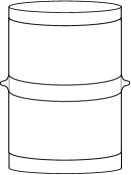
(b)

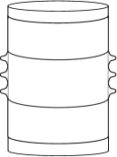
(c)

Figure 1.1. This figure depicts the three types of axisymmetric wrinkling patterns that achieve the minimum energy scaling laws from Theorem 1.1. In each, a thin elastic cylinder of unit radius and thickness $h$ is compressed axially by amount $\lambda$, and lies entirely outside of an inner cylindrical mandrel of radius $\varrho>1$. Pattern A shows the trivial wrinkling pattern, i.e., the unbuckled configuration, which achieves an excess energy scaling as $\lambda^{2}$. Pattern B is made up of one wrinkle, and achieves an excess energy scaling as $(\varrho-1)^{4/7}h^{6/7}\lambda^{5/7}$. Pattern C features many wrinkles, and achieves an excess energy scaling as $(\varrho-1)^{2/3}h^{2/3}\lambda$. In this pattern, the number of wrinkles scales as $(\varrho-1)^{1/3}h^{-2/3}\lambda$. A similar discussion applies for Theorem 1.3, where $\varrho-1$ is replaced by $(\varrho^{2}-1)\vee h^{2}$.

A similar result can be proved for the nonlinear energy. Define

(1.7) $$\mathcal{E}_{b}^{NL}(\varrho,h)=\left|\Omega\right|\left(\varrho^{2}-1\right)^{2}+\left|\Omega\right|\varrho^{2}h^{2}$$

and recall the definition of $c_{0}$ given immediately before the statement of Theorem 1.1 above.

Theorem 1.3.

Let $\varrho_{0}\in[1,\infty)$, and let $h,\lambda\in(0,\frac{1}{2}]$, $\varrho\in[1,\varrho_{0}]$, and $m\in[1,\infty)$. Then we have that

$$\min_{A_{\lambda,\varrho,m}^{NL}}E_{h}^{NL}-\mathcal{E}_{b}^{NL}\sim_{\varrho_{0},m}\min\left\{\lambda^{2},\max\left\{[(\varrho^{2}-1)\vee h^{2}]^{4/7}h^{6/7}\lambda^{5/7},[(\varrho^{2}-1)\vee h^{2}]^{2/3}h^{2/3}\lambda\right\}\right\}$$

whenever $(\varrho^{2}-1)\vee h^{2}\geq c_{0}(\lambda,h,1)$.

Remark 1.4.

In contrast with Theorem 1.1, we do not address the case $m=\infty$ in this result. As the reader will observe, our proof of the lower bound part of Theorem 1.3 rests on the assumption that $m<\infty$. However, in the proof of the upper bound part, the successful test functions belong to $A_{\lambda,\varrho,1}^{NL}$ uniformly in $h$. It does not appear to us that one can improve the scaling of these upper bounds by considering test functions with exploding slopes. This should be contrasted with the blow-up estimates discussed for the vKD model in Remark 1.2.

Proof.

Theorem 1.3 follows from Proposition 2.7 and Proposition 3.6 once we observe that

$$\lambda h\leq\max\{h^{6/7}\lambda^{5/7}[(\varrho^{2}-1)\vee h^{2}]^{4/7},[(\varrho^{2}-1)\vee h^{2}]^{2/3}\lambda h^{2/3}\}\iff\min\{\lambda^{1/2}h^{1/4},h^{1/2}\}\leq(\varrho^{2}-1)\vee h^{2}.$$

∎

1.2.2. The neutral mandrel case

Next we turn to the borderline case between the large and small mandrel cases, given by $\varrho=1$. In this case, our methods prove upper and lower bounds on the minimum energy which fail to match in general, though they do match in a regime in which the thickness, $h$, is large as compared to the compression, $\lambda$.

We begin with the results for the vKD model.

Theorem 1.5.

Let $h,\lambda\in(0,\frac{1}{2}]$ and $m\in[2,\infty)$. Then we have that

$$\min\left\{\max\{h\lambda^{3/2},(h\lambda)^{12/11}\},\lambda^{2}\right\}\lesssim_{m}\min_{A_{\lambda,1,m}^{vKD}}E_{h}^{vKD}\lesssim\min\left\{h\lambda,\lambda^{2}\right\}.$$

In the case that $m=\infty$, we have that

$$\min\left\{\max\{(h\lambda)^{12/11}\},\lambda^{2}\right\}\lesssim\min_{A_{\lambda,1,\infty}^{vKD}}E_{h}^{vKD}\lesssim\min\left\{h\lambda,\lambda^{2}\right\}.$$

Remark 1.6.

Although the lower bound in this result changes when $m=\infty$, in this case it does not imply a blow-up rate for $\lvert\lvert D\phi\rvert\rvert_{L^{\infty}}$ as $h\to 0$. Indeed, as discussed in Remark 2.6, minimizing sequences need not have exploding slopes in the neutral mandrel case.

Proof.

Taking $\varrho=1$ in Proposition 2.1 proves the upper bound part of Theorem 1.5. To prove the lower bound part, we first observe that if we define

(1.8) $$FS_{h}(\phi)=\int_{\Omega}\,\lvert\epsilon_{\theta\theta}\rvert^{2}+\lvert\epsilon_{zz}\rvert^{2}+h^{2}\lvert D^{2}\phi_{\rho}\rvert^{2}\,d\theta dz,$$

then

$$E_{h}^{vKD}(\phi)\geq FS_{h}(\phi)\quad\forall\,\phi\in A_{\lambda,\varrho,m}^{vKD}.$$

Proposition 4.1 identifies the minimum energy scaling law of $FS_{h}$ over $A_{\lambda,1,m}^{vKD}$, and this proves the result. ∎

As the reader will note, the argument in the proof above uses only the $\theta\theta$- and $zz$-components of the membrane term. As far as scaling is concerned, the lower bounds given in Theorem 1.5 are the optimal bounds that can be proved by such a method. This is discussed in more detail in Section 4.1; the essential point is that our lower bounds arise as the minimum energy scaling law of what we call the free-shear functional, defined in (1.8) above.

The upper and lower bounds from Theorem 1.5 match in a certain regime of the form $h\geq\lambda^{\alpha}$.

Corollary 1.7.

Let $h,\lambda\in(0,\frac{1}{2}]$ and $m\in[2,\infty)$. If $h\geq\lambda^{5/6}$, we have that

$$\min_{A_{\lambda,1,m}^{vKD}}E_{h}^{vKD}\sim_{m}\lambda^{2}.$$

The same result holds in the case that $m=\infty$.

Remark 1.8.

We note here a possible connection between our analysis and that of [11, 12], which derives Koiter’s formula for the incipient buckling load of a (perfect) thin cylinder via an analysis of the fully nonlinear model. Although our focus is not on buckling as such, Corollary 1.7 proves that, in the regime $\lambda\leq h^{6/5}$, the minimum energy scales as that of the unbuckled deformation. In comparison, the buckling load of a thin elastic cylinder scales linearly with $h$. If the effect of the neutral mandrel is to improve local to global stability, then perhaps the upper bound from Theorem 1.5 is optimal in its scaling.

Proof.

Corollary 1.7 follows from Theorem 1.5, after observing that, since $\lambda\leq 1$,

$$h\geq\lambda^{5/6}\iff\max\{h\lambda^{3/2},(h\lambda)^{12/11}\}\geq\lambda^{2}.$$

∎

Now we state the corresponding results for the nonlinear energy.

Theorem 1.9.

Let $h,\lambda\in(0,\frac{1}{2}]$ and $m\in[1,\infty)$. Then we have that

$$\min\left\{\max\left\{h\lambda^{3/2},(h\lambda)^{12/11}\right\},\lambda^{2}\right\}\lesssim_{m}\min_{A_{\lambda,1,m}^{NL}}E_{h}^{NL}-\mathcal{E}_{b}^{NL}(1,h)\lesssim_{\varrho_{0}}\min\left\{\lambda h,\lambda^{2}\right\}.$$

Remark 1.10.

As discussed in Remark 1.4, the lower bound in the case that $m=\infty$ is not addressed for the nonlinear model by our methods.

Proof.

Taking $\varrho=\varrho_{0}=1$ in Proposition 2.7 gives the upper bound part, once we observe that

$$\lambda\leq 1\implies\lambda h\geq\min\{h^{2}\lambda^{5/7},\lambda^{2}\}.$$

The lower bound part follows from Proposition 4.12.∎

Corollary 1.11.

Let $h,\lambda\in(0,\frac{1}{2}]$ and $m\in[1,\infty)$. If $h\geq\lambda^{5/6}$, then we have that

$$\min_{A_{\lambda,1,\infty}^{NL}}E_{h}^{NL}-\mathcal{E}_{b}^{NL}(1,h)\sim_{m}\lambda^{2}$$

Proof.

Arguing as in the proof of Corollary 1.7, we see that the result follows from Theorem 1.9. ∎

1.3. Discussion of the proofs

We turn now to a discussion of the mathematical ideas behind the proofs of these results. To fix ideas, we focus exclusively in this section on the nonlinear model, given in (1.4). For added clarity, we consider only the case where $h\to 0$ while $\lambda\in(0,\frac{1}{2}]$, $\varrho\in[1,\infty)$, and $m\in[1,\infty)$ are held fixed. Under these additional assumptions, Theorem 1.3 and Theorem 1.9 imply the following results:

• If $\varrho>1$, there are constants $c,C$ depending only on $\lambda,\varrho,m$ such that

  (1.9) $$ch^{2/3}\leq\min_{A_{\lambda,\varrho,m}^{NL}}E_{h}^{NL}-\mathcal{E}_{b}^{NL}\leq Ch^{2/3}\quad\text{as}\ h\to 0.$$

• If $\varrho=1$, there are constants $c,C$ depending only on $\lambda,m$ such that

  (1.10) $$ch\leq\min_{A_{\lambda,1,m}^{NL}}E_{h}^{NL}-\mathcal{E}_{b}^{NL}\leq Ch\quad\text{as}\ h\to 0.$$

1.3.1. The bulk energy

We see from (1.7) that $\mathcal{E}_{b}^{NL}$ is of the form

$$\mathcal{E}_{b}^{NL}=b_{m}(\varrho)+b_{\kappa}(\varrho)h^{2}.$$

The first factor, $b_{m}$, is the “bulk membrane energy” that remains in the limit $h\to 0$. The second factor, $b_{\kappa}h^{2}$, is the “bulk bending energy” and appears in $\mathcal{E}_{b}^{NL}$ due to our choice of bending term.

The bulk membrane energy can be found by solving the relaxed problem:

(1.11) $$b_{m}=\min_{\Phi\in A_{\lambda,\varrho,m}^{NL}}\int_{\Omega}QW(D\Phi)\,dx.$$

Here, $QW$ is the quasiconvexification of $W(F)=\left|F^{T}F-\text{id}\right|^{2}$. It follows from the results of [22] that

$$QW(F)=(\lambda_{1}^{2}-1)_{+}^{2}+(\lambda_{2}^{2}-1)_{+}^{2}$$

where $\{\lambda_{i}\}_{i=1,2}$ are the singular values of $F$.

Regardless of whether we consider the large, neutral, or small mandrel cases, the deformation

$$\Phi_{\text{eff}}(\theta,z)=(1+(\varrho-1)_{+},\theta,(1-\lambda)z)$$

is a minimizer of (1.11). The effective (first Piola–Kirchhoff) stress field is given by

(1.12) $$\sigma_{\text{eff}}=DQW(D\Phi_{\text{eff}})=4\varrho(\varrho^{2}-1)_{+}E_{\theta}\otimes e_{\theta},$$

and the bulk membrane energy satisfies

$$b_{m}=|\Omega|(\varrho^{2}-1)_{+}^{2}.$$

We note here that in the large mandrel case, where $\varrho>1$, both $\sigma_{\text{eff}}$ and $b_{m}$ are non-zero, whereas for the small or neutral mandrels these both vanish. As will become clear, the appearance of different power laws for the scaling of the excess energy in (1.9) and (1.10) is due precisely to the vanishing or non-vanishing of $\sigma_{\text{eff}}$.

1.3.2. Upper bounds

To achieve the upper bounds from (1.9) and (1.10), one must construct a good test function and estimate its elastic energy. The particular test functions that we use are of the form

(1.13) $$\Phi(\theta,z)=(\varrho+w(z),\theta,(1-\lambda)z+u(z)).$$

We refer to such constructions as “axisymmetric wrinkling patterns” (see Figure 1.1 on page 1.1). By construction, the metric tensor $g=D\Phi^{T}D\Phi$ satisfies $g_{\theta z}=0$ and by choosing $u,w$ suitably we can ensure that $g_{zz}=0$ as well.

In Section 2, we estimate the elastic energy of (1.13). The result is that the excess energy is bounded above by a multiple of

$$\int_{I_{z}}(\varrho^{2}-1)_{+}|w|+|w|^{2}+h^{2}|w^{\prime\prime}|^{2}\,dz,$$

where $\lvert\lvert w^{\prime}\rvert\rvert_{L^{2}}\geq c(\lambda)$. Minimizing over all such $w$ leads to the desired upper bounds. Evidently, both the character of the optimal $w$ and the scaling in $h$ of the resulting upper bound depend crucially on whether $\varrho>1$.

1.3.3. Ansatz-free lower bounds

The proofs of the lower bounds from (1.9) and (1.10) require an ansatz-free argument. We start by establishing the following claims:

1. With enough axial confinement, low-energy configurations must buckle;

2. Buckling in the presence of the mandrel induces excess hoop stress, and costs energy.

The first claim is quantified in Corollary 3.12, with the result being that low-energy configurations must satisfy

(1.14) $$\lvert\lvert D\Phi_{\rho}\rvert\rvert_{L^{2}}\geq c(\lambda).$$

The second claim is quantified in Lemma 3.8; this result implies in particular that the excess energy is bounded below by a multiple of

(1.15) $$(\varrho^{2}-1)_{+}\lvert\lvert\Phi_{\varrho}-\varrho\rvert\rvert_{L^{1}(\Omega)}+\lvert\lvert\Phi_{\rho}-\varrho\rvert\rvert_{L_{z}^{2}L_{\theta}^{1}}^{2}.$$

The anisotropic norm appearing here is characteristic of our neutral mandrel analysis. It arises because we consider the stretching of each $\theta$-hoop individually in this case, a choice that may be sub-optimal in general as it ignores the cost of shear.

Finally, we prove in Lemma 3.13 that, for low-energy configurations, the excess energy is bounded below by a multiple of

(1.16) $$h^{2}\lvert\lvert D^{2}\Phi_{\rho}\rvert\rvert_{L^{2}(\Omega)}^{2}.$$

While such a bound comes for free when we consider $E_{h}^{vKD}$, it requires some extra work for $E_{h}^{NL}$, due to the nonlinearities in the bending term.

Combining (1.14), (1.15), and (1.16) with various Gagliardo-Nirenberg interpolation inequalities (see Section 5), we conclude the desired lower bounds.

1.3.4. The role of $\sigma_{\text{eff}}$ in lower bounds

As described above, the vanishing of the effective applied stress, $\sigma_{\text{eff}}$, affects both the scaling law of the excess energy as well as the character of low energy sequences. We wish now to present a short argument for the first part of (1.15). While this argument is not strictly necessary for the proof of the main results, we believe that it helps to clarify the role of $\sigma_{\text{eff}}$ in the lower bounds.

It turns out that

$$E_{h}^{NL}(\Phi)-\mathcal{E}_{b}^{NL}\geq\int_{\Omega}W(D\Phi)-b_{m},$$

i.e., the excess energy can be split into its membrane and bending parts (see Lemma 3.7). Since $QW\leq W$, we have that

$$\int_{\Omega}W(D\Phi)-b_{m}\geq\int_{\Omega}QW(D\Phi)-QW(D\Phi_{eff}).$$

If $\sigma_{\text{eff}}\neq 0$, then to first order

(1.17) $$QW(D\Phi)-QW(D\Phi_{eff})=\left\langle\sigma_{\text{eff}},D(\Phi-\Phi_{\text{eff}})\right\rangle+h.o.t.,$$

and in fact we have that

$$QW(D\Phi)-QW(D\Phi_{\text{eff}})\geq\left\langle\sigma_{\text{eff}},D(\Phi-\Phi_{\text{eff}})\right\rangle$$

since $QW$ is convex (this also follows from [22]). Integrating by parts with the formula (1.12), and using that $\Phi_{\rho}\geq\varrho$, we conclude that

$$\int_{\Omega}\left\langle\sigma_{\text{eff}},D(\Phi-\Phi_{\text{eff}})\right\rangle=\int_{\Omega}|\sigma_{\text{eff}}||\Phi_{\rho}-\varrho|.$$

Hence,

$$E_{h}^{NL}(\Phi)-\mathcal{E}_{b}^{NL}\geq|\sigma_{\text{eff}}|\lvert\lvert\Phi_{\rho}-\varrho\rvert\rvert_{L^{1}(\Omega)}\quad\forall\,\Phi\in A_{\lambda,\varrho,\infty}^{NL}.$$

While this argument succeeds in proving the first part of (1.15), it fails to prove the second part since, essentially, the expansion (1.17) fails to capture the leading order behavior of $QW$ in the neutral mandrel case. Nevertheless, one can prove the full power of (1.15) assuming only that the cylinder is at least as large as the mandrel, i.e., $\varrho\geq 1$. The argument we give in Section 3.2 establishes both parts at once, using only familiar calculus and Sobolev-type inequalities along with the basic definitions.

1.4. Outline

In Section 2, we give the proofs of the upper bound parts of Theorem 1.1, Theorem 1.3, Theorem 1.5, and Theorem 1.9. In Section 3 we prove the lower bounds in the large mandrel case, i.e., the lower bound parts of Theorem 1.1 and Theorem 1.3. In Section 4, we consider the analysis of lower bounds in the neutral mandrel case. There, we prove the lower bound parts of Theorem 1.5 and Theorem 1.9, as well as the energy scaling law for the free-shear functional. We end with a short appendix in Section 5 which contains the various interpolation inequalities that we use.

1.5. Notation

The notation $X\lesssim Y$ means that there exists a positive numerical constant $C$ such that $X\leq CY$, and the notation $X\lesssim_{a}Y$ means that there exists a positive constant $C^{\prime}$ depending only on $a$ such that $X\leq C^{\prime}(a)Y$. The notation $X\sim Y$ means that $X\lesssim Y$ and $Y\lesssim X$, and similarly for $X\sim_{a}Y$.

When the meaning is clear, we sometimes abbreviate function spaces on $\Omega$ by dropping the dependence on the domain, e.g., $H^{k}=H^{k}(\Omega)$. The space $H_{\text{per}}^{k}=H_{\text{per}}^{k}(\Omega)$ is the space of periodic Sobolev functions on $\Omega$ of order $k$ and integrability $2$. We employ the following notation regarding mixed $L^{p}$-norms:

$$\lvert\lvert f\rvert\rvert_{L_{x_{1}}^{p_{1}}L_{x_{2}}^{p_{2}}}=\left(\int\left(\int|f(x_{1},x_{2})|^{p_{2}}\,dx_{2}\right)^{\frac{p_{1}}{p_{2}}}\,dx_{1}\right)^{\frac{1}{p_{1}}}$$

and

$$\lvert\lvert f\rvert\rvert_{L_{x_{1}}^{p}}(x_{2})=\left(\int|f(x_{1},x_{2})|^{p}\,dx_{1}\right)^{\frac{1}{p}}.$$

We refer to the unit basis vectors for the reference $\theta,z$-coordinates on $\Omega$ as $\{e_{i}\}_{i\in\{\theta,z\}}$, and the unit frame of coordinate vectors for the cylindrical $\rho,\theta,z$-coordinates on $\mathbb{R}^{3}$ as $\{E_{i}\}_{i\in\{\rho,\theta,z\}}$. Note that $E_{\rho}=E_{\rho}(x)$ and $E_{\theta}=E_{\theta}(x)$ depend on $x\in\mathbb{R}^{3}$ through its $\theta$-coordinate, $x_{\theta}$; our convention is that $E_{\rho}$ points in the direction of increasing radial coordinate, $\rho$, and $E_{\theta}$ in the direction of increasing azimuthal coordinate, $\theta$, so that in particular $x=x_{\rho}E_{\rho}(x)+x_{z}E_{z}$. We will sometimes perform Lebesgue averages of a function $f:\Omega\to\mathbb{R}$ over the reference $\theta$-coordinate. We denote this by

$$\overline{f}(z)=\frac{1}{\left|I_{\theta}\right|}\int_{I_{\theta}}f(\theta,z)\,d\theta.$$

The notation $\left|A\right|$ denotes the Euclidean volume of the (Lebesgue measurable) set $A$. The set $\mathcal{B}(U)$ denotes the set of Lebesgue measurable subsets $A\subset U$.

1.6. Acknowledgements

We would like to thank our advisor R. V. Kohn for his constant support. We would like to thank S. Conti for many inspirational discussions during an intermediate phase of this project, and in particular for his insight into the analysis of the free-shear functional. We would like to thank the University of Bonn for its hospitality during our visit in April and May of 2015. This research was conducted while the author was supported by a National Science Foundation Graduate Research Fellowship DGE-0813964, and National Science Foundation grants OISE-0967140 and DMS-1311833.

2. Elastic energy of axisymmetric wrinkling patterns

We begin our analysis of the compressed cylinder by estimating the elastic energy of various axisymmetric wrinkling patterns. This amounts to considering test functions that depend only on the $z$-coordinate. The results in this section constitute the upper bound parts of Theorem 1.1, Theorem 1.3, Theorem 1.5, and Theorem 1.9. We consider the vKD model in Section 2.1 and the nonlinear model in Section 2.2.

2.1. vKD model

Recall the definitions of $E_{h}^{vKD}$, $A_{\lambda,\varrho,m}^{vKD}$, and $\mathcal{E}_{b}^{vKD}$, given in (1.2), (1.3), and (1.6) respectively. In this section, we prove the following upper bound.

Proposition 2.1.

We have that

$$\min_{A_{\lambda,\varrho,m}^{vKD}}E_{h}^{vKD}-\mathcal{E}_{b}^{vKD}\lesssim\min\left\{\lambda^{2},\max\left\{\lambda h,h^{6/7}\lambda^{5/7}(\varrho-1)^{4/7},m^{-1/3}(\varrho-1)^{2/3}\lambda h^{2/3}\right\}\right\}$$

whenever $h,\lambda\in(0,\frac{1}{2}]$, $\varrho\in[1,\infty)$, and $m\in[2,\infty]$.

Proof.

The upper bound of $\lambda^{2}$ is achieved by the unbuckled configuration, $\phi=(\varrho-1,0,-\lambda z)$. To prove the remainder of the upper bound, note first that it suffices to achieve it for $(h,\lambda,\varrho,m)\in(0,h_{0}]\times(0,\frac{1}{2}]\times[1,\infty)\times[2,\infty]$ for some $h_{0}\in(0,\frac{1}{2}]$. We apply Lemma 2.3, Lemma 2.4, and Lemma 2.5 to deduce the required upper bound in the stated parameter range with $h_{0}=\frac{1}{2^{4}}$. ∎

In the remainder of this section, we will assume that

$$h\in(0,\frac{1}{2^{4}}],\ \lambda\in(0,\frac{1}{2}],\ \varrho\in[1,\infty),\ \text{and}\ m\in[2,\infty]$$

unless otherwise explicitly stated.

We begin by defining a two-scale axisymmetric wrinkling pattern. We will refer to the parameters $n\in\mathbb{N}$ and $\delta\in(0,1]$, which are the number of wrinkles and their relative extent. We refer the reader to Figure 2.1 on page 2.1 for a schematic of this construction.

Fix $f\in C^{\infty}(\mathbb{R})$ such that

• $f$ is non-negative and one-periodic

• $\text{supp}\,f\cap[-\frac{1}{2},\frac{1}{2}]\subset(-\frac{1}{2},\frac{1}{2})$

• $\lvert\lvert f^{\prime}\rvert\rvert_{L^{\infty}}\leq 2$

• $\lvert\lvert f^{\prime}\rvert\rvert_{L^{2}(B_{1/2})}^{2}=1$,

and define $f_{\delta,n}\in C^{\infty}(\mathbb{R})$ by

$$f_{\delta,n}(t)=\frac{\sqrt{\delta}}{n}f(\frac{n}{\delta}\{t\})\mathbbm{1}_{\{t\}\in B_{\delta/2}}.$$

Define $w_{\delta,n,\lambda},u_{\delta,n,\lambda}:\Omega\to\mathbb{R}$ by

$$w_{\delta,n,\lambda}(\theta,z)=\sqrt{2\lambda}f_{\delta,n}(z)\quad\text{and}\quad u_{\delta,n,\lambda}(\theta,z)=\int_{-\frac{1}{2}\leq z^{\prime}\leq z}\lambda-\frac{1}{2}(\partial_{z}w_{\delta,n,\lambda}(\theta,z^{\prime}))^{2}\,dz^{\prime}.$$

Finally, define $\phi_{\delta,n,\lambda,\varrho}:\Omega\to\mathbb{R}^{3}$ by

$$\phi_{\delta,n,\lambda,\varrho}=(w_{\delta,n,\lambda}+\varrho-1,0,-\lambda z+u_{\delta,n,\lambda}),$$

in cylindrical coordinates.

Figure 2.1. This schematic depicts the axisymmetric wrinkle construction used in the proof of the upper bounds. The pattern features $n$ wrinkles in the $e_{z}$-direction with volume fraction $\delta$. The optimal choice of $\delta,n$ depends on the axial compression, $\lambda$, the thickness, $h$, the mandrel’s radius, $\varrho$, and the a priori $L^{\infty}$ slope bound, $m$.

Now, we estimate the elastic energy of this construction in the vKD model. Define

$$m_{1}(\lambda,\delta)=2\max\left\{\sqrt{\frac{2\lambda}{\delta}},\frac{2\lambda}{\delta}\right\}.$$

Lemma 2.2.

We have that $\phi_{\delta,n,\lambda,\varrho}\in A_{\lambda,\varrho,m_{1}}^{vKD}$. Furthermore,

$$E_{h}^{vKD}(\phi_{\delta,n,\lambda,\varrho})-\mathcal{E}_{b}^{vKD}\lesssim\max\left\{(\varrho-1)\frac{\lambda^{1/2}\delta^{3/2}}{n},\frac{\lambda\delta^{2}}{n^{2}},h^{2}\frac{\lambda n^{2}}{\delta^{2}}\right\}.$$

Proof.

Abbreviate $\phi_{\delta,n,\lambda,\varrho}$ by $\phi$, $w_{\delta,n,\lambda}$ by $w$, and $u_{\delta,n,\lambda}$ by $u$. We claim that $\phi_{\rho}\in H_{\text{per}}^{2}$, $\phi_{\theta}\in H_{\text{per}}^{1}$, and $\phi_{z}+\lambda z\in H_{\text{per}}^{1}$. To see this, observe that

$$\int_{I_{z}}\frac{1}{2}|\partial_{z}w_{\delta,n,\lambda}|^{2}dz=\lambda\int_{B_{\delta/2}}|f^{\prime}_{\delta,n}|^{2}dt=\lambda\int_{B_{1/2}}|f^{\prime}|^{2}dt=\lambda$$

for all $\theta\in I_{\theta}$, so that $u\in H_{\text{per}}^{1}$. That $w\in H_{\text{per}}^{2}$ follows from its definition. Observe also that $\phi_{\rho}\geq\varrho-1$, since $w\geq 0$.

Now we check the slope bounds. By construction, we have that

$$\epsilon_{zz}=\partial_{z}\phi_{z}+\frac{1}{2}(\partial_{z}\phi_{\rho})^{2}=0$$

and that

$$\partial_{z}\phi_{\rho}=\partial_{z}w=\sqrt{2\lambda}f^{\prime}_{\delta,n}.$$

Hence,

$$\lvert\lvert\partial_{z}\phi_{\rho}\rvert\rvert_{L^{\infty}}\leq\sqrt{2\lambda}\lvert\lvert f_{\delta,n}^{\prime}\rvert\rvert_{L^{\infty}}\leq 2\sqrt{\frac{2\lambda}{\delta}}$$

and

$$\lvert\lvert\partial_{z}\phi_{z}\rvert\rvert_{L^{\infty}}\leq\lambda\lvert\lvert f^{\prime}_{\delta,n}\rvert\rvert_{L^{\infty}}^{2}\leq\frac{4\lambda}{\delta}.$$

It follows that

$$\max_{\begin{subarray}{c}i\in\left\{\theta,z\right\},\,j\in\{\rho,\theta,z\}\end{subarray}}\lvert\lvert\partial_{i}\phi_{j}\rvert\rvert_{L^{\infty}}\leq m_{1}(\lambda,\delta),$$

and therefore that $\phi\in A_{\lambda,\varrho,m_{1}}^{vKD}$.

Now we bound the elastic energy of this construction. Since $\epsilon_{zz}=\epsilon_{\theta z}=0$ and $w$ depends only on $z$, we see that

$$E_{h}^{vKD}(\phi)=\int_{\Omega}\,\lvert w+\varrho-1\rvert^{2}+h^{2}\lvert\partial_{z}^{2}w\rvert^{2}\,d\theta dz$$

and hence that

$$E_{h}^{vKD}(\phi)-\mathcal{E}_{b}^{vKD}\lesssim\max\left\{(\varrho-1)_{+}\lvert\lvert w\rvert\rvert_{L^{1}(\Omega)},\lvert\lvert w\rvert\rvert_{L^{2}(\Omega)}^{2},h^{2}\lvert\lvert\partial_{z}^{2}w\rvert\rvert_{L^{2}(\Omega)}^{2}\right\}.$$

Now we conclude the desired result from the elementary bounds

$$\lvert\lvert w\rvert\rvert_{L^{1}(\Omega)}\lesssim\frac{\lambda^{1/2}\delta^{3/2}}{n},\quad\lvert\lvert w\rvert\rvert_{L^{2}(\Omega)}^{2}\lesssim\frac{\lambda\delta^{2}}{n^{2}},\ \text{and}\quad\lvert\lvert\partial_{z}^{2}w\rvert\rvert_{L^{2}(\Omega)}^{2}\lesssim\frac{\lambda n^{2}}{\delta^{2}}.$$

∎

We make three choices of the parameters $n,\delta$ in what follows. First, we consider a construction which features many wrinkles as $h\to 0$.

Lemma 2.3.

Assume that $m<\infty$ and that

$$m^{-1/3}(\varrho-1)^{2/3}\lambda h^{2/3}\geq\max\{\lambda h,h^{6/7}\lambda^{5/7}(\varrho-1)^{4/7}\}.$$

Let $n\in\mathbb{N}$ and $\delta\in(0,1]$ satisfy

$$n\in\left[(\varrho-1)^{1/3}\lambda h^{-2/3}m^{-7/6},2(\varrho-1)^{1/3}\lambda h^{-2/3}m^{-7/6}\right]\quad\text{and}\quad\delta=4\lambda m^{-1}.$$

Then, $\phi_{\delta,n,\lambda,\varrho}\in A_{\lambda,\varrho,m}^{vKD}$ and

$$E_{h}^{vKD}(\phi_{\delta,n,\lambda,\varrho})-\mathcal{E}_{b}^{vKD}\lesssim\frac{(\varrho-1)^{2/3}h^{2/3}\lambda}{m^{1/3}}.$$

Proof.

Rearranging the inequality $m^{-1/3}(\varrho-1)^{2/3}\lambda h^{2/3}\geq h^{6/7}\lambda^{5/7}(\varrho-1)^{4/7}$, we find that $(\varrho-1)^{1/3}\lambda h^{-2/3}m^{-7/6}\geq 1$ so that there exists such an $n\in\mathbb{N}$. Also, with our choice of $\delta$ we have that $m_{1}(\delta,\lambda)=m.$ We note that indeed $\delta\leq 1$ since $\lambda\leq\frac{1}{2}$ and $m\geq 2$.

It follows from Lemma 2.2 that $\phi_{\delta,n,\lambda,\varrho}\in A_{\lambda,\varrho,m}^{vKD}$, and that

$$E_{h}^{vKD}(\phi_{\delta,n,\lambda,\varrho})-\mathcal{E}_{b}^{vKD}\lesssim\max\left\{(\varrho-1)^{2/3}h^{2/3}m^{7/6}\delta^{3/2}\frac{1}{\lambda^{1/2}},\frac{\delta^{2}h^{4/3}m^{7/3}}{(\varrho-1)^{2/3}\lambda},h^{2/3}\frac{\lambda^{3}(\varrho-1)^{2/3}}{\delta^{2}m^{7/3}}\right\}.$$

Using that $\delta\sim\frac{\lambda}{m}$, we have that

$$E_{h}^{vKD}(\phi_{\delta,n,\lambda,\varrho})-\mathcal{E}_{b}^{vKD}\lesssim\max\left\{\frac{(\varrho-1)^{2/3}h^{2/3}\lambda}{m^{1/3}},\lambda m^{1/3}\frac{h^{4/3}}{(\varrho-1)^{2/3}}\right\}.$$

Since

$$\frac{(\varrho-1)^{2/3}h^{2/3}\lambda}{m^{1/3}}\geq\lambda m^{1/3}\frac{h^{4/3}}{(\varrho-1)^{2/3}}\iff(\varrho-1)^{2/3}\geq m^{1/3}h^{1/3},$$

the result follows. ∎

Next, we consider a construction consisting of one wrinkle.

Lemma 2.4.

Assume that

$$h^{6/7}\lambda^{5/7}(\varrho-1)^{4/7}\geq\max\{\lambda h,m^{-1/3}(\varrho-1)^{2/3}\lambda h^{2/3}\}.$$

Let $n=1$ and let $\delta\in(0,1]$ be given by

$$\delta=4\lambda^{1/7}(\varrho-1)^{-2/7}h^{4/7}.$$

Then, $\phi_{\delta,n,\lambda,\varrho}\in A_{\lambda,\varrho,m}^{vKD}$ and

$$E_{h}^{vKD}(\phi_{\delta,n,\lambda,\varrho})-\mathcal{E}_{b}^{vKD}\lesssim h^{6/7}\lambda^{5/7}(\varrho-1)^{4/7}.$$

Proof.

First, we check that $\delta\leq 1$. Note that $4\lambda^{1/7}h^{4/7}(\varrho-1)^{-2/7}\leq 1$ if and only if $\lambda h^{4}\leq(\varrho-1)^{2}\frac{1}{2^{14}}$. By assumption, we have that $\lambda h\leq h^{6/7}\lambda^{5/7}(\varrho-1)^{4/7}$ so that $\lambda h^{1/2}\leq(\varrho-1)^{2}$. Since $h\leq\frac{1}{2^{4}}$, it follows that $h^{4}\leq\frac{1}{2^{14}}h^{1/2}$ and hence that $\lambda h^{4}\leq\frac{1}{2^{14}}(\varrho-1)^{2}$ as required.

Now we check the slope bounds. We have that

$$m_{1}(\lambda,\delta)=\max\left\{\sqrt{2}\lambda^{3/7}(\varrho-1)^{1/7}h^{-2/7},\lambda^{6/7}(\varrho-1)^{2/7}h^{-4/7}\right\}.$$

By assumption, $m^{-1/3}(\varrho-1)^{2/3}\lambda h^{2/3}\leq h^{6/7}\lambda^{5/7}(\varrho-1)^{4/7}$ so that $(\varrho-1)^{2/7}\lambda^{6/7}h^{-4/7}\leq m$. Since $m\geq 2$, we have that $m^{2}\geq 2m$ so that $2(\varrho-1)^{2/7}\lambda^{6/7}h^{-4/7}\leq 2m\leq m^{2}$ and hence $\sqrt{2}(\varrho-1)^{1/7}\lambda^{3/7}h^{-2/7}\leq m$. It follows that $m_{1}(\lambda,\delta)\leq m$.

Using Lemma 2.2, we conclude that $\phi_{\delta,n,\lambda,\varrho}\in A_{\lambda,\varrho,m}^{vKD}$ and that

$$E_{h}^{vKD}(\phi)-\mathcal{E}_{b}^{vKD}\lesssim\max\left\{(\varrho-1)^{4/7}\lambda^{5/7}h^{6/7},\lambda^{9/7}(\varrho-1)^{-4/7}h^{8/7}\right\}.$$

Since

$$(\varrho-1)^{4/7}\lambda^{5/7}h^{6/7}\geq\lambda^{9/7}(\varrho-1)^{-4/7}h^{8/7}\iff(\varrho-1)^{2}\geq\lambda h^{1/2}$$

we conclude the desired result. ∎

The previous two results fail to cover the neutral mandrel case, where $\varrho=1$. Our next result includes this case.

Lemma 2.5.

Assume that

$$\lambda h\geq\max\{m^{-1/3}(\varrho-1)^{2/3}\lambda h^{2/3},h^{6/7}\lambda^{5/7}(\varrho-1)^{4/7}\}.$$

If $\lambda\leq mh^{1/2}$, then upon taking $n=1$ and $\delta=4h^{1/2}\in(0,1]$ we find that $\phi_{\delta,n,\lambda,\varrho}\in A_{\lambda,\varrho,m}^{vKD}$ and that

$$E_{h}^{vKD}(\phi_{\delta,n,\lambda,\varrho})-\mathcal{E}_{b}^{vKD}\lesssim\lambda h.$$

If $\lambda>mh^{1/2}$, then upon taking $n\in\mathbb{N}$ and $\delta\in(0,1]$ which satisfy

$$n\in[\lambda h^{-1/2}m^{-1},2\lambda h^{-1/2}m^{-1}]\quad\text{and}\quad\delta=4\lambda m^{-1},$$

we find that $\phi_{\delta,n,\lambda,\varrho}\in A_{\lambda,\varrho,m}^{vKD}$ and that

$$E_{h}^{vKD}(\phi_{\delta,n,\lambda,\varrho})-\mathcal{E}_{b}^{vKD}\lesssim\lambda h.$$

Remark 2.6.

We note here that if $\varrho-1$ is small enough, then the scaling law of $\lambda h$ can be achieved by a construction with uniformly bounded slopes. Indeed, if one takes $n\sim h^{-1/2}$ and $\delta=1$, then the resulting $\phi_{\delta,n,\lambda,\varrho}$ belongs to $A_{\lambda,\varrho,m}^{vKD}$ for all $\lambda\in[0,\frac{1}{2}]$ and $m\in[2,\infty]$, and the excess energy is bounded by a multiple of $\lambda h$ whenever $\varrho-1\leq\lambda^{1/2}h^{1/2}$.

Proof.

We prove this in two parts. Assume first that $\lambda\leq mh^{1/2}$. Then let $n=1$ and $\delta=4h^{1/2}$. Note that $\delta\in(0,1]$ if and only if $h\leq\frac{1}{2^{4}}$. Also,

$$m_{1}(\lambda,\delta)=\max\left\{2\sqrt{\frac{2\lambda}{4h^{1/2}}},\frac{4\lambda}{4h^{1/2}}\right\}=\max\left\{\sqrt{\frac{2\lambda}{h^{1/2}}},\frac{\lambda}{h^{1/2}}\right\}.$$

Since $m\geq 2$, $2m\leq m^{2}$. Thus, $\lambda\leq mh^{1/2}\implies 2\lambda\leq 2mh^{1/2}\leq m^{2}h^{1/2}$ so that $(2\lambda h^{-1/2})^{1/2}\leq m$. Thus, $m_{1}(\lambda,\delta)\leq m$. By Lemma 2.2, we have that $\phi_{\delta,n,\lambda,\varrho}\in A_{\lambda,\varrho,m}^{vKD}$ and that

$$E_{h}^{vKD}(\phi_{\delta,n,\lambda,\varrho})-\mathcal{E}_{b}^{vKD}\lesssim\max\left\{(\varrho-1)\lambda^{1/2}h^{3/4},\lambda h\right\}.$$

Note that $(\varrho-1)\lambda^{1/2}h^{3/4}\leq\lambda h$ is a rearrangement of $\lambda h\geq h^{6/7}\lambda^{5/7}(\varrho-1)^{4/7}$. Thus,

$$E_{h}^{vKD}(\phi_{\delta,n,\lambda,\varrho})-\mathcal{E}_{b}^{vKD}\lesssim\lambda h.$$

Now assume that $\lambda>mh^{1/2}$. Let $n\in\mathbb{N}$ and $\delta\in(0,1]$ satisfy

$$n\in[\lambda h^{-1/2}m^{-1},2\lambda h^{-1/2}m^{-1}]\quad\text{and}\quad\delta=4\lambda m^{-1}.$$

Note that $\lambda h^{-1/2}m^{-1}>1$ is a rearrangement of $\lambda>h^{1/2}m$, so that such an $n$ exists. Also, note that $\delta\leq 1$ since $m\geq 2$ and $\lambda\leq\frac{1}{2}$, and that $m_{1}(\delta,\lambda)=m$. Hence by Lemma 2.2, we have that $\phi_{\delta,n,\lambda,\varrho}\in A_{\lambda,\varrho,m}^{vKD}$ and that

$$E_{h}^{vKD}(\phi_{\delta,n,\lambda,\varrho})-\mathcal{E}_{b}^{vKD}\lesssim\max\left\{(\varrho-1)\frac{\lambda h^{1/2}}{m^{1/2}},\lambda h\right\}.$$

Since $(\varrho-1)\frac{\lambda h^{1/2}}{m^{1/2}}\leq\lambda h$ is a rearrangement of $\lambda h\geq m^{-1/3}(\varrho-1)^{2/3}\lambda h^{2/3}$, we conclude that

$$E_{h}^{vKD}(\phi_{\delta,n,\lambda,\varrho})-\mathcal{E}_{b}^{vKD}\lesssim\lambda h.$$

∎

2.2. Nonlinear model

Recall the definitions of $E_{h}^{NL}$, $A_{\lambda,\varrho,m}^{NL}$, and $\mathcal{E}_{b}^{NL}$, given in (1.4), (1.5), and (1.7). In this section, we prove the following upper bound.

Proposition 2.7.

Let $\varrho_{0}\in[1,\infty)$. Then we have that

$$\min_{A_{\lambda,\varrho,m}^{NL}}E_{h}^{NL}-\mathcal{E}_{b}^{NL}\lesssim_{\varrho_{0}}\min\left\{\lambda^{2},\max\left\{\lambda h,h^{6/7}\lambda^{5/7}[(\varrho^{2}-1)\vee h^{2}]^{4/7},[(\varrho^{2}-1)\vee h^{2}]^{2/3}\lambda h^{2/3}\right\}\right\}$$

whenever $h,\lambda\in(0,\frac{1}{2}]$, $\varrho\in[1,\varrho_{0}]$, and $m\in[1,\infty]$.

Proof.

Note that since $A_{\lambda,\varrho,m}^{NL}\subset A_{\lambda,\varrho,m^{\prime}}^{NL}$ if $m\leq m^{\prime}$, we only need to prove the claim for the case of $m=1$. The upper bound of $\lambda^{2}$ is achieved by the unbuckled configuration, $\Phi=(\varrho,\theta,(1-\lambda)z)$. To prove the remainder of the upper bound, note first that it suffices to achieve it for $(h,\lambda,\varrho)\in(0,h_{0}]\times(0,\frac{1}{2}]\times[1,\varrho_{0}]$ for some $h_{0}\in(0,\frac{1}{2}]$. We apply Lemma 2.9, Lemma 2.10, and Lemma 2.11 to deduce the required upper bound in the stated parameter range with $h_{0}=\frac{1}{4}$. Note that the dependence of the constants in these lemmas on $f$ can be dropped, since $f$ is fixed in the subsequent paragraphs. ∎

In the remainder of this section, we fix $\varrho_{0}\in[1,\infty)$ as in the claim. Furthermore, we assume that

$$h\in(0,\frac{1}{4}],\ \lambda\in(0,\frac{1}{2}],\ \text{and}\quad\varrho\in[1,\varrho_{0}]$$

unless otherwise explicitly stated.

As in the analysis of the vKD model, we define a two-scale axisymmetric wrinkling pattern. We refer to $n\in\mathbb{N}$ and $\delta\in(0,1]$, which represent the number of wrinkles and their relative extent respectively. Again, we refer the reader to Figure 2.1 on page 2.1 for a schematic of this construction.

We start by fixing $f\in C^{\infty}(\mathbb{R})$ such that

• $f$ is non-negative and one-periodic

• $\text{supp}\,f\cap[-\frac{1}{2},\frac{1}{2}]\subset(-\frac{1}{2},\frac{1}{2})$

• $\lvert\lvert f^{\prime}\rvert\rvert_{L^{\infty}}<1$

• $\int_{-\frac{1}{2}}^{\frac{1}{2}}\sqrt{1-f^{\prime 2}}\,dt=\frac{1}{2}$.

Define $f_{\delta,n}\in C^{\infty}(\mathbb{R})$ by

$$f_{\delta,n}(t)=\frac{\delta}{n}f(\frac{n}{\delta}\{t\})\mathbbm{1}_{\{t\}\in B_{\delta/2}}.$$

Let $S_{f}:[0,1]\to\mathbb{R}$ be defined by

$$S_{f}(q)=1-\int_{-\frac{1}{2}}^{\frac{1}{2}}\sqrt{1-q^{2}f^{\prime 2}}\,dt,$$

and observe that $S_{f}$ is a bijection of $[0,1]\leftrightarrow[0,\frac{1}{2}]$. Hence, if $\delta\in[2\lambda,1]$, we can define $w_{\delta,n,\lambda},u_{\delta,n,\lambda}:\Omega\to\mathbb{R}$ by

$$w_{\delta,n,\lambda}(\theta,z)=S_{f}^{-1}\left(\frac{\lambda}{\delta}\right)f_{\delta,n}(z)\quad\text{and}\quad u_{\delta,n,\lambda}(\theta,z)=\int_{-\frac{1}{2}\leq z^{\prime}\leq z}\sqrt{1-(\partial_{z}w_{\delta,n,\lambda}(\theta,z^{\prime}))^{2}}-(1-\lambda)\,dz^{\prime}.$$

Finally, we define $\Phi_{\delta,n,\lambda,\varrho}:\Omega\to\mathbb{R}^{3}$ by

$$\Phi_{\delta,n,\lambda,\varrho}=(w_{\delta,n,\lambda}+\varrho,\theta,(1-\lambda)z+u_{\delta,n,\lambda}),$$

in cylindrical coordinates.

We now estimate the elastic energy of this wrinkling pattern.

Lemma 2.8.

Let $\delta\in[2\lambda,1]$. Then we have that $\Phi_{\delta,n,\lambda,\varrho}\in A_{\lambda,\varrho,1}^{NL}$. Furthermore,

$$E_{h}^{NL}(\Phi_{\delta,n,\lambda,\varrho})-\mathcal{E}_{b}^{NL}\lesssim_{\varrho_{0},f}\max\left\{\left[(\varrho^{2}-1)\vee h^{2}\right]\frac{\lambda^{1/2}\delta^{3/2}}{n},\frac{\lambda\delta^{2}}{n^{2}},h^{2}\frac{\lambda n^{2}}{\delta^{2}}\right\}.$$

Proof.

Abbreviate $\Phi_{\delta,n,\lambda,\varrho}$ by $\Phi$, $w_{\delta,n,\lambda}$ by $w$, and $u_{\delta,n,\lambda}$ by $u$. By its definition, $\Phi_{\rho}\in H_{\text{per}}^{2}$, $\Phi_{\theta}-\theta\in H_{\text{per}}^{2}$, and $\Phi_{z}-(1-\lambda)z\in H_{\text{per}}^{2}$. To see these, note that $w,u\in H_{\text{per}}^{2}$. Indeed, we have that

$$\int_{-\frac{1}{2}}^{\frac{1}{2}}\sqrt{1-(\partial_{z}w(\theta,z))^{2}}\,dz =\int_{[-\frac{1}{2},\frac{1}{2}]\backslash B_{\delta/2}}1\,dt+\int_{B_{\delta/2}}\sqrt{1-\left(S_{f}^{-1}\left(\frac{\lambda}{\delta}\right)f_{\delta,n}^{\prime}(t)\right)^{2}}\,dt$$

$$=2(\frac{1}{2}-\frac{\delta}{2})+\delta\int_{-\frac{1}{2}}^{\frac{1}{2}}\sqrt{1-(S_{f}^{-1}\left(\frac{\lambda}{\delta}\right))^{2}\left(f^{\prime}(t)\right)^{2}}\,dt$$

$$=1-\delta S_{f}\circ S_{f}^{-1}(\frac{\lambda}{\delta})=1-\lambda$$

for each $\theta\in I_{\theta}$. Also, we have that $\Phi_{\rho}\geq\varrho$, since $w\geq 0$, and that

$$\partial_{z}\Phi_{z}=1-\lambda+\partial_{z}u=\sqrt{1-(\partial_{z}w)^{2}}\geq 0.$$

Now we check the slope bounds. Note that

$$\partial_{z}\Phi_{\rho}=\partial_{z}w=S_{f}^{-1}\left(\frac{\lambda}{\delta}\right)f_{\delta,n}^{\prime}(z)$$

so that

$$\lvert\lvert\partial_{z}\Phi_{\rho}\rvert\rvert_{L^{\infty}}\leq\left|S_{f}^{-1}\left(\frac{\lambda}{\delta}\right)\right|\lvert\lvert f_{\delta,n}^{\prime}\rvert\rvert_{L^{\infty}}\leq\lvert\lvert f^{\prime}\rvert\rvert_{L^{\infty}}<1.$$

Also, by the above, we have that

$$\partial_{z}\Phi_{z}=\sqrt{1-(\partial_{z}w)^{2}}\in[0,1].$$

Hence,

$$\max_{\begin{subarray}{c}i\in\left\{\theta,z\right\},\,j\in\{\rho,\theta,z\}\end{subarray}}\lvert\lvert\partial_{i}\Phi_{j}\rvert\rvert_{L^{\infty}}\leq 1$$

and it follows that $\Phi\in A_{\lambda,\varrho,1}^{NL}$.

Now we bound the energy of this construction. Since $g_{zz}=1$, $g_{\theta z}=0$, and $u,w$ are functions of $z$ alone, we have that

$$E_{h}^{NL}(\Phi)=\int_{\Omega}\,\left|(\varrho+w)^{2}-1\right|^{2}+h^{2}(\left|\varrho+w\right|^{2}+|\partial_{z}^{2}w|^{2}+2|\partial_{z}w|^{2}+|\partial_{z}^{2}u|^{2})\,d\theta dz.$$

Hence,

$$E_{h}^{NL}(\Phi)-\mathcal{E}_{b}^{NL}\lesssim_{\varrho_{0}} \max\{\left[(\varrho^{2}-1)\vee h^{2}\right]\lvert\lvert w\rvert\rvert_{L^{1}(\Omega)},\lvert\lvert w\rvert\rvert_{L^{2}(\Omega)}^{2},$$

$$\qquad h^{2}\left(\lvert\lvert\partial_{z}^{2}w\rvert\rvert_{L^{2}(\Omega)}^{2}\vee\lvert\lvert\partial_{z}w\rvert\rvert_{L^{2}(\Omega)}^{2}\vee\lvert\lvert\partial_{z}^{2}u\rvert\rvert_{L^{2}(\Omega)}^{2}\right)\}.$$

(Here we used that $\lvert\lvert w\rvert\rvert_{L^{\infty}}\leq 1$, which follows from its definition and our choice of $f$.) By definition, we have that

$$\partial_{z}^{2}u=-\frac{\partial_{z}w\partial_{z}^{2}w}{\sqrt{1-(\partial_{z}w)^{2}}}$$

so that

$$\lvert\lvert\partial_{z}u\rvert\rvert_{L^{2}(\Omega)}\lesssim_{f}\lvert\lvert\partial_{z}^{2}w\rvert\rvert_{L^{2}(\Omega)}.$$

Also, we have that

$$\lvert\lvert w\rvert\rvert_{L^{1}(\Omega)}\lesssim S_{f}^{-1}(\frac{\lambda}{\delta})\frac{\delta^{2}}{n},\quad\lvert\lvert w\rvert\rvert_{L^{2}(\Omega)}^{2}\lesssim\left(S_{f}^{-1}(\frac{\lambda}{\delta})\right)^{2}\frac{\delta^{3}}{n^{2}},$$

$$\lvert\lvert\partial_{z}w\rvert\rvert_{L^{2}(\Omega)}^{2}\lesssim\left(S_{f}^{-1}(\frac{\lambda}{\delta})\right)^{2}\delta,\ \text{and}\quad\lvert\lvert\partial_{z}^{2}w\rvert\rvert_{L^{2}(\Omega)}^{2}\lesssim\left(S_{f}^{-1}(\frac{\lambda}{\delta})\right)^{2}\frac{n^{2}}{\delta}.$$

Since

$$\frac{q^{2}}{2}\lvert\lvert f^{\prime}\rvert\rvert_{L^{2}([-\frac{1}{2},\frac{1}{2}])}^{2}\leq S_{f}(q)$$

it follows that

$$S_{f}^{-1}(\frac{\lambda}{\delta})\lesssim_{f}\left(\frac{\lambda}{\delta}\right)^{1/2}.$$

Combining the above, we conclude that

$$E_{h}^{NL}(\Phi)-\mathcal{E}_{b}^{NL}\lesssim_{\varrho_{0},f}\max\left\{\left[(\varrho^{2}-1)\vee h^{2}\right]\frac{\lambda^{1/2}\delta^{3/2}}{n},\frac{\lambda\delta^{2}}{n^{2}},h^{2}\left(\frac{\lambda n^{2}}{\delta^{2}}\vee\lambda\right)\right\}$$

and the result immediately follows. ∎

Next, we choose $n,\delta$ which are optimal for our construction in various regimes. Our first choice exhibits many wrinkles, and is the nonlinear analog of Lemma 2.3.

Lemma 2.9.

Assume that

$$[(\varrho^{2}-1)\vee h^{2}]^{2/3}\lambda h^{2/3}\geq\max\{\lambda h,h^{6/7}\lambda^{5/7}[(\varrho^{2}-1)\vee h^{2}]^{4/7}\}.$$

Let $n\in\mathbb{N}$ and $\delta\in(0,1]$ satisfy

$$n\in\left[[(\varrho^{2}-1)\vee h^{2}]^{1/3}\lambda h^{-2/3},2[(\varrho^{2}-1)\vee h^{2}]^{1/3}\lambda h^{-2/3}\right]\quad\text{and}\quad\delta=2\lambda.$$

Then, $\Phi_{\delta,n,\lambda,\varrho}\in A_{\lambda,\varrho,1}^{NL}$ and

$$E_{h}^{NL}(\Phi_{\delta,n,\lambda,\varrho})-\mathcal{E}_{b}^{NL}\lesssim_{\varrho_{0},f}[(\varrho^{2}-1)\vee h^{2}]^{2/3}\lambda h^{2/3}.$$

Proof.

Rearranging the inequality $[(\varrho^{2}-1)\vee h^{2}]^{2/3}\lambda h^{2/3}\geq h^{6/7}\lambda^{5/7}[(\varrho^{2}-1)\vee h^{2}]^{4/7}$, we find that $[(\varrho^{2}-1)\vee h^{2}]^{1/3}\lambda h^{-2/3}\geq 1$ so that there exists such an $n\in\mathbb{N}$. Also, with our choice of $\delta$ we have that $\delta\in[2\lambda,1]$. It follows immediately from Lemma 2.8 that $\Phi_{\delta,n,\lambda,\varrho}\in A_{\lambda,\varrho,1}^{NL}$. Finally, the bound on the energy follows from Lemma 2.8 as in the proof of Lemma 2.3, where $\varrho-1$ is replaced by $(\varrho^{2}-1)\vee h^{2}$ and $m$ is replaced by the number $1$. ∎

Next, we consider a pattern consisting of one wrinkle.

Lemma 2.10.

Assume that

$$h^{6/7}\lambda^{5/7}[(\varrho^{2}-1)\vee h^{2}]^{4/7}\geq\max\{\lambda h,[(\varrho^{2}-1)\vee h^{2}]^{2/3}\lambda h^{2/3}\}.$$

Let $n=1$ and let $\delta\in[2\lambda,1]$ be given by

$$\delta=2\lambda^{1/7}[(\varrho^{2}-1)\vee h^{2}]^{-2/7}h^{4/7}.$$

Then, $\Phi_{\delta,n,\lambda,\varrho}\in A_{\lambda,\varrho,1}^{NL}$ and

$$E_{h}^{NL}(\Phi_{\delta,n,\lambda,\varrho})-\mathcal{E}_{b}^{NL}\lesssim_{\varrho_{0},f}h^{6/7}\lambda^{5/7}[(\varrho^{2}-1)\vee h^{2}]^{4/7}.$$

Proof.

First, we check that $\delta\in[2\lambda,1]$. For the upper bound, note that $2\lambda^{1/7}[(\varrho^{2}-1)\vee h^{2}]^{-2/7}h^{4/7}\leq 1$ if and only if $\lambda h^{4}\leq\frac{1}{2^{7}}[(\varrho^{2}-1)\vee h^{2}]^{2}$. By assumption, we have that $\lambda h\leq h^{6/7}\lambda^{5/7}[(\varrho^{2}-1)\vee h^{2}]^{4/7}$ so that $\lambda h^{1/2}\leq[(\varrho^{2}-1)\vee h^{2}]^{2}$. Since $h\leq\frac{1}{4}$, it follows that $h^{4}\leq\frac{1}{2^{7}}h^{1/2}$ and hence that $\lambda h^{4}\leq\frac{1}{2^{7}}[(\varrho^{2}-1)\vee h^{2}]^{2}$ as required. For the lower bound, we note that $2\lambda^{1/7}[(\varrho^{2}-1)\vee h^{2}]^{-2/7}h^{4/7}\geq 2\lambda$ if and only if $h^{4}\geq\lambda^{6}[(\varrho^{2}-1)\vee h^{2}]^{2}$. As this is a rearrangement of $[(\varrho^{2}-1)\vee h^{2}]^{2/3}\lambda h^{2/3}\leq h^{6/7}\lambda^{5/7}[(\varrho^{2}-1)\vee h^{2}]^{4/7}$, we conclude the lower bound.

It follows from Lemma 2.8 that $\Phi_{\delta,n,\lambda,\varrho}\in A_{\lambda,\varrho,1}^{NL}$. The bound on the energy also follows from Lemma 2.8, as in the proof of Lemma 2.4 but where $\varrho-1$ is replaced by $(\varrho^{2}-1)\vee h^{2}$. ∎

Finally, we discuss the neutral mandrel case, where $\varrho=1$.

Lemma 2.11.

Assume that

$$\lambda h\geq\max\{[(\varrho^{2}-1)\vee h^{2}]^{2/3}\lambda h^{2/3},h^{6/7}\lambda^{5/7}[(\varrho^{2}-1)\vee h^{2}]^{4/7}\}.$$

If $\lambda\leq h^{1/2}$, then upon taking $n=1$ and $\delta=2h^{1/2}\in[2\lambda,1]$ we find that $\Phi_{\delta,n,\lambda,\varrho}\in A_{\lambda,\varrho,1}^{NL}$ and that

$$E_{h}^{NL}(\Phi_{\delta,n,\lambda,\varrho})-\mathcal{E}_{b}^{NL}\lesssim_{\varrho_{0},f}\lambda h.$$

If $\lambda>h^{1/2}$, then upon taking $n\in\mathbb{N}$ and $\delta\in[2\lambda,1]$ which satisfy

$$n\in[\lambda h^{-1/2},2\lambda h^{-1/2}]\quad\text{and}\quad\delta=2\lambda,$$

we find that $\Phi_{\delta,n,\lambda,\varrho}\in A_{\lambda,\varrho,1}^{NL}$ and that

$$E_{h}^{NL}(\Phi_{\delta,n,\lambda,\varrho})-\mathcal{E}_{b}^{NL}\lesssim_{\varrho_{0},f}\lambda h.$$

Proof.

We prove this in two parts. Assume first that $\lambda\leq h^{1/2}$. Then let $n=1$ and $\delta=2h^{1/2}$. Note that $\delta\in[2\lambda,1]$ if and only if $h\leq\frac{1}{4}$ and $h^{1/2}\geq\lambda$. It follows from Lemma 2.8 that $\Phi_{\delta,n,\lambda,\varrho}\in A_{\lambda,\varrho,1}^{NL}$, and the bound on the energy follows from Lemma 2.8 as in the proof of Lemma 2.5, where $\varrho-1$ is replaced by $(\varrho^{2}-1)\vee h^{2}$.

Now assume that $\lambda>h^{1/2}$. Let $n\in\mathbb{N}$ and $\delta\in[2\lambda,1]$ which satisfy

$$n\in[\lambda h^{-1/2},2\lambda h^{-1/2}]\quad\text{and}\quad\delta=2\lambda.$$

Note that $\lambda h^{-1/2}>1$ is a rearrangement of $\lambda>h^{1/2}$, so that such an $n$ exists. It follows immediately from Lemma 2.8 that $\Phi_{\delta,n,\lambda,\varrho}\in A_{\lambda,\varrho,1}^{NL}$. The bound on the energy follows from Lemma 2.8 as in the proof of Lemma 2.5, where $\varrho-1$ is replaced by $(\varrho^{2}-1)\vee h^{2}$ and $m$ is replaced by the number $1$. ∎

3. Ansatz-free lower bounds in the large mandrel case

We turn now to prove the ansatz-free lower bounds from Theorem 1.1 and Theorem 1.3. The key idea behind their proof is that buckling in the presence of the mandrel requires “outwards” displacement, i.e., displacement in the direction of increasing $\rho$, and that this results in the presence of non-trivial tensile hoop stresses. This observation leads to lower bounds on $E_{h}^{vKD}$ in Section 3.1 and on $E_{h}^{NL}$ in Section 3.2. These bounds are optimal in certain regimes of the form $\varrho-1\geq c_{m}(\lambda,h)>0$ (for the precise statement, we refer the reader to Section 1.2.1 in the introduction).

3.1. vKD model

Recall the definitions of $E_{h}^{vKD}$, $A_{\lambda,\varrho,m}^{vKD}$, and $\mathcal{E}_{b}^{vKD}$ from (1.2), (1.3), and (1.6). In Section 3.1.1, we prove the following lower bound.

Proposition 3.1.

We have that

$$\min\left\{\max\left\{m^{-2/3}(\varrho-1)^{2/3}h^{2/3}\lambda,\lambda^{5/7}(\varrho-1)^{4/7}h^{6/7}\right\},\lambda^{2}\right\}\lesssim\min_{A_{\lambda,\varrho,m}^{vKD}}E_{h}^{vKD}-\mathcal{E}_{b}^{vKD}$$

whenever $h,\lambda\in(0,\infty)$, $\varrho\in[1,\infty)$, and $m\in(0,\infty]$.

Proof.

This follows from Corollary 3.3 and Corollary 3.4, which combine to prove the equivalent statement that

$$\min_{A_{\lambda,\varrho,m}^{vKD}}E_{h}^{vKD}-\mathcal{E}_{b}^{vKD}\gtrsim\max\left\{\min\{m^{-2/3}(\varrho-1)^{2/3}h^{2/3}\lambda,\lambda^{2}\},\min\{\lambda^{5/7}(\varrho-1)^{4/7}h^{6/7},\lambda^{2}\}\right\}.$$

∎

In Section 3.1.2, we prove an estimate on the blow-up rate of $D\phi$ as $h\to 0$ for the minimizers of the $m=\infty$ problem.

3.1.1. Proof of the ansatz-free lower bound

We begin by controlling various features of the radial displacement, $\phi_{\rho}$. Given $\phi\in A_{\lambda,\varrho,m}^{vKD}$ we call

$$\Delta^{vKD}=E_{h}^{vKD}(\phi)-\mathcal{E}_{b}^{vKD},$$

which is the excess elastic energy in the vKD model.

Lemma 3.2.

Let $\phi\in A_{\lambda,\varrho,\infty}^{vKD}$. Then we have that

$$\Delta^{vKD}\geq\max\left\{(\varrho-1)\lvert\lvert\phi_{\rho}-(\varrho-1)\rvert\rvert_{L^{1}(\Omega)},h^{2}\lvert\lvert D^{2}\phi_{\rho}\rvert\rvert_{L^{2}(\Omega)}^{2},\lvert\lvert\frac{1}{2}\lvert\lvert\partial_{z}\phi_{\rho}\rvert\rvert_{L_{z}^{2}}^{2}-\lambda\rvert\rvert_{L_{\theta}^{2}}^{2}\right\}.$$

Proof.

Make the substitution

$$\phi=(w+\varrho-1,u_{\theta},u_{z}-\lambda z),$$

given in cylindrical coordinates. By definition, the vKD strain tensor, $\epsilon$, satisfies

$$\epsilon_{\theta\theta}=\partial_{\theta}u_{\theta}+\frac{1}{2}(\partial_{\theta}w)^{2}+w+(\varrho-1)\quad\text{and}\quad\epsilon_{zz}=\partial_{z}u_{z}-\lambda+\frac{1}{2}(\partial_{z}w)^{2}.$$

Since $u_{\theta}\in H_{\text{per}}^{1}$, we have that

$$E_{h}^{vKD}(\phi) \geq\int_{\Omega}\lvert\epsilon_{\theta\theta}\rvert^{2}+\lvert\epsilon_{zz}\rvert^{2}+h^{2}\lvert D^{2}w\rvert^{2}$$

$$\geq\int_{\Omega}(\varrho-1)^{2}+2(\varrho-1)(\partial_{\theta}u_{\theta}+\frac{1}{2}(\partial_{\theta}w)^{2}+w)+\lvert\epsilon_{zz}\rvert^{2}+h^{2}\lvert D^{2}w\rvert^{2}$$

$$\geq\mathcal{E}_{b}^{vKD}+\int_{\Omega}2(\varrho-1)w+\lvert\epsilon_{zz}\rvert^{2}+h^{2}\lvert D^{2}w\rvert^{2}.$$

Since $w$ is non-negative, we conclude that

$$\Delta^{vKD}\geq\max\left\{2(\varrho-1)\lvert\lvert w\rvert\rvert_{L^{1}(\Omega)},\lvert\lvert\epsilon_{zz}\rvert\rvert_{L^{2}(\Omega)}^{2},h^{2}\lvert\lvert D^{2}w\rvert\rvert_{L^{2}(\Omega)}^{2}\right\}.$$

By applying Jensen’s inequality and using that $u_{z}\in H_{\text{per}}^{1}$, it follows that

$$\lvert\lvert\epsilon_{zz}\rvert\rvert_{L^{2}(\Omega)}^{2}\geq\frac{1}{\lvert I_{z}\rvert}\int_{I_{\theta}}\lvert\int_{I_{z}}\epsilon_{zz}\,dz\rvert^{2}\,d\theta=\frac{1}{\lvert I_{z}\rvert}\lvert\lvert\frac{1}{2}\lvert\lvert\partial_{z}w\rvert\rvert_{L_{z}^{2}}^{2}-\lambda\rvert\rvert_{L_{\theta}^{2}}^{2}.$$

Since $\lvert I_{z}\rvert=1$, the result follows. ∎

Now, we will apply the Gagliardo-Nirenberg interpolation inequalities from Section 5 to deduce the desired lower bounds.

Corollary 3.3.

If $\phi\in A_{\lambda,\varrho,m}^{vKD}$, then

$$\Delta^{vKD}\gtrsim\min\{m^{-2/3}(\varrho-1)^{2/3}h^{2/3}\lambda,\lambda^{2}\}.$$

In fact, if $\phi\in A_{\lambda,\varrho,\infty}^{vKD}$, then

$$\Delta^{vKD}\gtrsim\min\{\lvert\lvert D\phi_{\rho}\rvert\rvert_{L^{\infty}}^{-2/3}(\varrho-1)^{2/3}h^{2/3}\lambda,\lambda^{2}\}.$$

Proof.

Observe that by Lemma 3.2 and an application of Hölder’s inequality, we have that

$$(\Delta^{vKD})^{1/2}\geq\lvert I_{z}\rvert^{-1/2}|I_{\theta}|^{-1/2}\lvert\lvert\frac{1}{2}\lvert\lvert\partial_{z}\phi_{\rho}\rvert\rvert_{L_{z}^{2}}^{2}-\lambda\rvert\rvert_{L_{\theta}^{1}}.$$

Hence, by the triangle inequality,

$$\frac{1}{2}\lvert\lvert\partial_{z}\phi_{\rho}\rvert\rvert_{L^{2}(\Omega)}^{2}+|\Omega|^{1/2}(\Delta^{vKD})^{1/2}\geq\lambda|I_{\theta}|.$$

Now we perform a case analysis. If $\phi$ satisfies $\lvert\lvert\partial_{z}\phi_{\rho}\rvert\rvert_{L^{2}(\Omega)}^{2}\leq\lambda|I_{\theta}|$, then we conclude by the above that $\Delta^{vKD}\gtrsim\lambda^{2}$.

If, on the other hand, $\phi$ satisfies $\lvert\lvert\partial_{z}\phi_{\rho}\rvert\rvert_{L^{2}(\Omega)}^{2}>\lambda|I_{\theta}|$, then we can combine the interpolation inequality from Lemma 5.2 (applied to $f=\phi_{\rho}-(\varrho-1)$) with Lemma 3.2 to conclude that

$$\lambda\lesssim\lvert\lvert D\phi_{\rho}\rvert\rvert_{L^{\infty}(\Omega)}^{2/3}\left(\frac{1}{\varrho-1}\Delta^{vKD}\right)^{2/3}\left(\frac{1}{h^{2}}\Delta^{vKD}\right)^{1/3}\lesssim m^{2/3}(\varrho-1)^{-2/3}h^{-2/3}\Delta^{vKD}.$$

These observations combine to prove the desired result.∎

Corollary 3.4.

If $\phi\in A_{\lambda,\varrho,m}^{vKD}$, then

$$\Delta^{vKD}\gtrsim\min\{\lambda^{5/7}(\varrho-1)^{4/7}h^{6/7},\lambda^{2}\}.$$

Proof.

Evidently, it suffices to prove that

$$\Delta^{vKD}\leq|I_{\theta}|\lambda^{2}\implies\Delta^{vKD}\gtrsim\lambda^{5/7}(\varrho-1)^{4/7}h^{6/7}.$$

Assume that $\Delta^{vKD}\leq|I_{\theta}|\lambda^{2}$, and define the set

$$Z=\left\{\theta\in I_{\theta}\ :\ \lvert\frac{1}{2}\lvert\lvert\partial_{z}\phi_{\rho}\rvert\rvert_{L_{z}^{2}}^{2}-\lambda\rvert\geq\sqrt{2}\lambda\right\}.$$

We claim that $|I_{\theta}\backslash Z|\geq\frac{1}{2}|I_{\theta}|$. Indeed, by Chebyshev’s inequality and Lemma 3.2, we have that

$$2\lambda^{2}\lvert Z\rvert\leq\lvert\lvert\frac{1}{2}\lvert\lvert\partial_{z}\phi_{\rho}\rvert\rvert_{L_{z}^{2}}^{2}-\lambda\rvert\rvert_{L_{\theta}^{2}}^{2}\leq|I_{\theta}|\lambda^{2}$$

so that $|Z|\leq\frac{1}{2}|I_{\theta}|$ as desired. It follows that

$$\lambda^{5/7}\lvert I_{\theta}\rvert\lesssim\int_{I_{\theta}\backslash Z}\lvert\lvert\partial_{z}\phi_{\rho}\rvert\rvert_{L_{z}^{2}}^{10/7}\,d\theta\leq\int_{I_{\theta}}\lvert\lvert\partial_{z}\phi_{\rho}\rvert\rvert_{L_{z}^{2}}^{10/7}\,d\theta.$$

Applying the first interpolation inequality from Lemma 5.1 to $f=\phi_{\rho}-(\varrho-1)$, we conclude that

$$\lambda^{5/7}\lvert I_{\theta}\rvert\lesssim\int_{I_{\theta}}\lvert\lvert f\rvert\rvert_{L_{z}^{1}}^{4/7}\lvert\lvert\partial_{z}^{2}f\rvert\rvert_{L_{z}^{2}}^{6/7}\,d\theta\leq\lvert\lvert\phi_{\rho}-(\varrho-1)\rvert\rvert_{L^{1}(\Omega)}^{4/7}\lvert\lvert D^{2}\phi_{\rho}\rvert\rvert_{L^{2}(\Omega)}^{6/7}.$$

Note that we used Hölder’s inequality in the second step. Finally, Lemma 3.2 proves that

$$\lambda^{5/7}\lesssim\left(\frac{1}{\varrho-1}\Delta^{vKD}\right)^{4/7}\left(\frac{1}{h^{2}}\Delta^{vKD}\right)^{3/7}=(\varrho-1)^{-4/7}h^{-6/7}\Delta^{vKD}$$

and the lower bound follows. ∎

3.1.2. Blow-up rate of $D\phi$ as $h\to 0$

We can now make Remark 1.2 precise, regarding the claim that $E_{h}^{vKD}$ prefers exploding slopes in the limit $h\to 0$. The following result can be seen to justify the introduction of the parameter $m$ in the definition of the admissible set, $A_{\lambda,\varrho,m}^{vKD}$.

Corollary 3.5.

Let $\left\{(h_{\alpha},\lambda_{\alpha},\varrho_{\alpha})\right\}_{\alpha\in\mathbb{R}_{+}}$ be such that $h_{\alpha},\lambda_{\alpha}\in(0,\frac{1}{2}]$ and $\varrho_{\alpha}\geq 1+\lambda_{\alpha}^{1/2}h_{\alpha}^{1/4}$. Assume that $h_{\alpha}\ll(\varrho_{\alpha}-1)^{-2/3}\lambda_{\alpha}^{3/2}$ as $\alpha\to\infty$, and let $\{\phi^{\alpha}\}_{\alpha\in\mathbb{R}_{+}}$ satisfy

$$\phi^{\alpha}\in A_{\lambda_{\alpha},\varrho_{\alpha},\infty}^{vKD}\quad\text{and}\quad E_{h_{\alpha}}^{vKD}(\phi^{\alpha})=\min_{A_{\lambda_{\alpha},\varrho_{\alpha},\infty}^{vKD}}E_{h_{\alpha}}^{vKD}.$$

Then we have that

$$(\varrho_{\alpha}-1)^{1/7}h_{\alpha}^{-2/7}\lambda_{\alpha}^{3/7}\lesssim\lvert\lvert D\phi_{\rho}^{\alpha}\rvert\rvert_{L^{\infty}}\quad\text{as}\ \alpha\to\infty.$$

Proof.

For ease of notation, we omit the index $\alpha$ in what follows. By Proposition 2.1 we have that

$$E_{h}^{vKD}(\phi)-\mathcal{E}_{b}^{vKD}\lesssim h^{6/7}\lambda^{5/7}(\varrho-1)^{4/7}.$$

Hence, by Corollary 3.3, it follows that

$$\lambda^{2}\lesssim h^{6/7}\lambda^{5/7}(\varrho-1)^{4/7}\quad\text{or}\quad\lvert\lvert D\phi_{\rho}\rvert\rvert_{L^{\infty}}^{-2/3}(\varrho-1)^{2/3}h^{2/3}\lambda\lesssim h^{6/7}\lambda^{5/7}(\varrho-1)^{4/7}.$$

Rearranging, we have that

$$h\gtrsim(\varrho-1)^{-2/3}\lambda^{3/2}\quad\text{or}\quad(\varrho-1)^{1/7}h^{-2/7}\lambda^{3/7}\lesssim\lvert\lvert D\phi_{\rho}\rvert\rvert_{L^{\infty}}.$$

By assumption the first inequality does not hold, and the result follows. ∎

3.2. Nonlinear model

Recall the definitions of $E_{h}^{NL}$, $A_{\lambda,\varrho,m}^{NL}$, and $\mathcal{E}_{b}^{NL}$ given in (1.4), (1.5), and (1.7). In this section, we prove the following lower bound.

Proposition 3.6.

Let $\varrho_{0}\in[1,\infty)$. Then we have that

$$\min\left\{\max\left\{\left[(\varrho^{2}-1)\vee h^{2}\right]^{2/3}h^{2/3}\lambda,\lambda^{5/7}[(\varrho^{2}-1)\vee h^{2}]^{4/7}h^{6/7}\right\},\lambda^{2}\right\}\lesssim_{m,\varrho_{0}}\min_{A_{\lambda,\varrho,m}^{NL}}E_{h}^{NL}-\mathcal{E}_{b}^{NL}$$

whenever $h,\lambda\in(0,1]$, $\varrho\in[1,\varrho_{0}]$, and $m\in(0,\infty)$.

The reader may notice that, although it is certainly more involved, the following argument shares the same overall structure as the one given for the vKD model in Section 3.1. For more on this, we refer to the discussion in Section 1.3.

In the remainder of this section, we assume that

$$0<h,\lambda\leq 1,\quad 1\leq\varrho\leq\varrho_{0}<\infty,\ \text{and}\quad 0<m<\infty.$$

Given $\Phi\in A_{\lambda,\varrho,m}^{NL}$ we call

(3.1) $$\Delta^{NL}=E_{h}^{NL}(\Phi)-\mathcal{E}_{b}^{NL},$$

which is the excess elastic energy in the nonlinear model. Observe we may assume that

$$\Phi\ \text{satisfies}\ \Delta^{NL}\leq 1,$$

since otherwise the desired bound is clear. As the reader will note, this assumption simplifies the discussion throughout.

We will make frequent use of the following identities concerning the components of the metric tensor, $g=D\Phi^{T}D\Phi$, in $(\theta,z)$-coordinates:

(3.2) $$\begin{split}g_{\theta\theta}&=\left(\partial_{\theta}\Phi_{\rho}\right)^{2}+\Phi_{\rho}^{2}\left(\partial_{\theta}\Phi_{\theta}\right)^{2}+\left(\partial_{\theta}\Phi_{z}\right)^{2}\\ g_{zz}&=\left(\partial_{z}\Phi_{\rho}\right)^{2}+\Phi_{\rho}^{2}\left(\partial_{z}\Phi_{\theta}\right)^{2}+\left(\partial_{z}\Phi_{z}\right)^{2}\\ g_{\theta z}&=\partial_{\theta}\Phi_{\rho}\partial_{z}\Phi_{\rho}+\Phi_{\rho}^{2}\partial_{\theta}\Phi_{\theta}\partial_{z}\Phi_{\theta}+\partial_{\theta}\Phi_{z}\partial_{z}\Phi_{z}\end{split}$$

We will also make use of the following identities concerning the components of $D^{2}\Phi$ in $(\theta,z)$-coordinates:

(3.3) $$\begin{split}\partial_{\theta}^{2}\Phi&=(\partial_{\theta}^{2}\Phi_{\rho}-\Phi_{\rho}(\partial_{\theta}\Phi_{\theta})^{2})E_{\rho}(\Phi)+(2\partial_{\theta}\Phi_{\rho}\partial_{\theta}\Phi_{\theta}+\Phi_{\rho}\partial_{\theta}^{2}\Phi_{\theta})E_{\theta}(\Phi)+\partial_{\theta}^{2}\Phi_{z}E_{z}\\ \partial_{z}^{2}\Phi&=(\partial_{z}^{2}\Phi_{\rho}-\Phi_{\rho}(\partial_{z}\Phi_{\theta})^{2})E_{\rho}(\Phi)+(2\partial_{z}\Phi_{\rho}\partial_{z}\Phi_{\theta}+\Phi_{\rho}\partial_{z}^{2}\Phi_{\theta})E_{\theta}(\Phi)+\partial_{z}^{2}\Phi_{z}E_{z}\\ \partial_{\theta z}\Phi&=(\partial_{\theta z}\Phi_{\rho}-\Phi_{\rho}\partial_{\theta}\Phi_{\theta}\partial_{z}\Phi_{\theta})E_{\rho}(\Phi)+(\partial_{\theta}\Phi_{\rho}\partial_{z}\Phi_{\theta}+\partial_{\theta}\Phi_{\theta}\partial_{z}\Phi_{\rho}+\Phi_{\rho}\partial_{\theta z}\Phi_{\theta})E_{\theta}(\Phi)+\partial_{\theta z}\Phi_{z}E_{z}\end{split}$$

Here, $\{E_{i}\}_{i\in\{\rho,\theta,z\}}$ denotes the unit frame of coordinate vectors for the cylindrical $\rho,\theta,z$-coordinates on $\mathbb{R}^{3}$ (as defined in Section 1.5).

3.2.1. Controlling the radial deformation

We begin by proving that the excess energy controls the membrane and bending terms individually.

Lemma 3.7.

If $\Phi\in A_{\lambda,\varrho,\infty}^{NL}$, then

$$\Delta^{NL} \geq\max\left\{\int_{\Omega}\lvert g_{\theta\theta}-1\rvert^{2}-(\varrho^{2}-1)^{2},\lvert\lvert g_{\theta z}\rvert\rvert_{L^{2}(\Omega)}^{2},\lvert\lvert g_{zz}-1\rvert\rvert_{L^{2}(\Omega)}^{2}\right\}$$

$$\Delta^{NL} \geq h^{2}\max\left\{\int_{\Omega}\lvert\partial_{\theta}^{2}\Phi\rvert^{2}-\varrho^{2},\lvert\lvert\partial_{\theta z}\Phi\rvert\rvert_{L^{2}(\Omega)}^{2},\lvert\lvert\partial_{z}^{2}\Phi\rvert\rvert_{L^{2}(\Omega)}^{2}\right\}.$$

Proof.

By the definition of $\Delta^{NL}$ in (3.1), it suffices to prove the following two inequalities to conclude the result:

$$\int_{\Omega}\lvert g_{\theta\theta}-1\rvert^{2}-(\varrho^{2}-1)^{2}\geq 0\quad\text{and}\quad\int_{\Omega}\lvert\partial_{\theta}^{2}\Phi\rvert^{2}-\varrho^{2}\geq 0.$$

To see the first inequality, we begin by noting that

(3.4) $$(g_{\theta\theta}-1)^{2}-(\varrho^{2}-1)^{2}=2(\varrho^{2}-1)(g_{\theta\theta}-\varrho^{2})+(g_{\theta\theta}-\varrho^{2})^{2}$$

and

(3.5) $$g_{\theta\theta}-\varrho^{2}=(\partial_{\theta}\Phi_{\rho})^{2}+\Phi_{\rho}^{2}(\partial_{\theta}\Phi_{\theta})^{2}+(\partial_{\theta}\Phi_{z})^{2}-\varrho^{2}$$

by (3.2). It follows that

(3.6) $$(g_{\theta\theta}-1)^{2}-(\varrho^{2}-1)^{2}\geq 2(\varrho^{2}-1)(\Phi_{\rho}^{2}(\partial_{\theta}\Phi_{\theta})^{2}-\varrho^{2}+(\partial_{\theta}\Phi_{\rho})^{2}+(\partial_{\theta}\Phi_{z})^{2}).$$

Using the hypothesis that $\Phi_{\rho}\geq\varrho$ and applying Jensen’s inequality, we see that

(3.7) $$\int_{\Omega}\Phi_{\rho}^{2}(\partial_{\theta}\Phi_{\theta})^{2}-\varrho^{2}\geq\frac{\varrho^{2}}{\left|\Omega\right|}\left(\left(\int_{\Omega}\partial_{\theta}\Phi_{\theta}\right)^{2}-\left|\Omega\right|^{2}\right)=\frac{\varrho^{2}}{\left|\Omega\right|}\left(\left|\Omega\right|^{2}-\left|\Omega\right|^{2}\right)=0.$$

Since $\varrho\geq 1$, the first inequality follows.

To see the second inequality, note that by (3.3) we have that

$$\lvert\partial_{\theta}^{2}\Phi\rvert\geq\lvert\partial_{\theta}^{2}\Phi_{\rho}-\Phi_{\rho}(\partial_{\theta}\Phi_{\theta})^{2}\rvert.$$

Hence, by Jensen’s inequality and since $\Phi_{\rho}\in H_{\text{per}}^{2}$, it follows that

$$\int_{\Omega}\lvert\partial_{\theta}^{2}\Phi\rvert^{2}-\varrho^{2}\geq\frac{1}{\lvert\Omega\rvert}\left(\int_{\Omega}\partial_{\theta}^{2}\Phi_{\rho}-\Phi_{\rho}(\partial_{\theta}\Phi_{\theta})^{2}\right)^{2}-\lvert\Omega\rvert\varrho^{2}=\frac{1}{\lvert\Omega\rvert}\left(\int_{\Omega}\Phi_{\rho}(\partial_{\theta}\Phi_{\theta})^{2}\right)^{2}-\lvert\Omega\rvert\varrho^{2}.$$

Using that $\Phi_{\rho}\geq\varrho$ and applying Jensen’s inequality again, we conclude that

$$\int_{\Omega}\lvert\partial_{\theta}^{2}\Phi\rvert^{2}-\varrho^{2}\geq\frac{\varrho^{2}}{|\Omega|}\left(\left(\int_{\Omega}(\partial_{\theta}\Phi_{\theta})^{2}\right)^{2}-\lvert\Omega\rvert^{2}\right)\geq\frac{\varrho^{2}}{|\Omega|}\left(|\Omega|^{2}-|\Omega|^{2}\right)=0$$

as desired. ∎

Next, we establish control on the radial component of the deformation, $\Phi_{\rho}$. As we will require the uniform-in-mandrel estimates from this result to complete the proof of Proposition 3.6, we record these alongside the large mandrel estimates now.

Lemma 3.8.

Let $\Phi\in A_{\lambda,\varrho,\infty}^{NL}$. Then we have that

$$\Delta^{NL} \gtrsim(\varrho^{2}-1)\max\{\lvert\lvert\Phi_{\rho}-\varrho\rvert\rvert_{L^{1}(\Omega)},\lvert\lvert\partial_{\theta}\Phi_{\rho}\rvert\rvert_{L^{2}(\Omega)}^{2},\lvert\lvert\partial_{\theta}\Phi_{\theta}-1\rvert\rvert_{L^{2}(\Omega)}^{2},\lvert\lvert\partial_{\theta}\Phi_{z}\rvert\rvert_{L^{2}(\Omega)}^{2}\}$$

$$(\Delta^{NL})^{1/2} \gtrsim\max\left\{\lvert\lvert\Phi_{\rho}-\varrho\rvert\rvert_{L_{z}^{2}L_{\theta}^{1}},\lvert\lvert\partial_{\theta}\Phi_{\rho}\rvert\rvert_{L_{z}^{4}L_{\theta}^{2}}^{2},\lvert\lvert\partial_{\theta}\Phi_{\theta}-1\rvert\rvert_{L_{z}^{4}L_{\theta}^{2}}^{2},\lvert\lvert\partial_{\theta}\Phi_{z}\rvert\rvert_{L_{z}^{4}L_{\theta}^{2}}^{2}\right\}.$$

Proof.

We begin by proving the first estimate. Recall Lemma 3.7 and equations (3.6) and (3.7). Altogether, these imply that

(3.8) $$\Delta^{NL}\geq 2(\varrho^{2}-1)\max\left\{\int_{\Omega}\Phi_{\rho}^{2}(\partial_{\theta}\Phi_{\theta})^{2}-\varrho^{2},\lvert\lvert\partial_{\theta}\Phi_{\rho}\rvert\rvert_{L^{2}(\Omega)}^{2},\lvert\lvert\partial_{\theta}\Phi_{z}\rvert\rvert_{L^{2}(\Omega)}^{2}\right\}.$$

Introduce the displacements $\phi_{\rho}=\Phi_{\rho}-\varrho$ and $\phi_{\theta}=\Phi_{\theta}-\theta$. In these variables,

(3.9) $$\Phi_{\rho}^{2}(\partial_{\theta}\Phi_{\theta})^{2}-\varrho^{2}\geq\varrho^{2}\left(2\partial_{\theta}\phi_{\theta}+(\partial_{\theta}\phi_{\theta})^{2}\right)+2\varrho\phi_{\rho}(\partial_{\theta}\phi_{\theta}+1)^{2}.$$

Since the second term is non-negative, and since $\phi_{\theta}\in H_{\text{per}}^{2}$ and $\varrho\geq 1$, we conclude from (3.9) that

(3.10) $$I:=\int_{\Omega}\Phi_{\rho}^{2}(\partial_{\theta}\Phi_{\theta})^{2}-\varrho^{2}\geq\int_{\Omega}\varrho^{2}\left(2\partial_{\theta}\phi_{\theta}+(\partial_{\theta}\phi_{\theta})^{2}\right)\geq\lvert\lvert\partial_{\theta}\phi_{\theta}\rvert\rvert_{L^{2}(\Omega)}^{2}.$$

In a similar manner, we can conclude from (3.9) that

$$I\geq\int_{\Omega}2\varrho\phi_{\rho}(\partial_{\theta}\phi_{\theta}+1)^{2}\geq\int_{\Omega}\phi_{\rho}(2\partial_{\theta}\phi_{\theta}+1)$$

and, since $\phi_{\rho}\geq 0$, that

$$I+\left|\int_{\Omega}\phi_{\rho}\partial_{\theta}\phi_{\theta}\right|\gtrsim\lvert\lvert\phi_{\rho}\rvert\rvert_{L^{1}(\Omega)}.$$

Recall the notation $\overline{f}$ for the $\theta$-average of a function $f$, introduced in Section 1.5. Integrating by parts and applying Poincare’s inequality, we see that

$$\lvert\int_{\Omega}\phi_{\rho}\partial_{\theta}\phi_{\theta}\rvert =\lvert\int_{\Omega}\partial_{\theta}\phi_{\rho}(\phi_{\theta}-\overline{\phi_{\theta}})\rvert\leq\lvert\lvert\partial_{\theta}\phi_{\rho}\rvert\rvert_{L^{2}(\Omega)}\lvert\lvert\phi_{\theta}-\overline{\phi_{\theta}}\rvert\rvert_{L^{2}(\Omega)}$$

$$\lesssim\lvert\lvert\partial_{\theta}\phi_{\rho}\rvert\rvert_{L^{2}(\Omega)}\lvert\lvert\partial_{\theta}\phi_{\theta}\rvert\rvert_{L^{2}(\Omega)}.$$

Hence,

(3.11) $$I+\lvert\lvert\partial_{\theta}\phi_{\rho}\rvert\rvert_{L^{2}(\Omega)}\lvert\lvert\partial_{\theta}\phi_{\theta}\rvert\rvert_{L^{2}(\Omega)}\gtrsim\lvert\lvert\phi_{\rho}\rvert\rvert_{L^{1}(\Omega)}.$$

Combining (3.8), (3.10), and (3.11) gives the required bound.

We turn now to prove the second estimate. First, we observe that by (3.5) and (3.7),

$$\int_{\Omega}g_{\theta\theta}-\varrho^{2}\geq\int_{\Omega}\Phi_{\rho}^{2}(\partial_{\theta}\Phi_{\theta})^{2}-\varrho^{2}\geq 0.$$

Hence, by Lemma 3.7, (3.4), and since $\varrho\geq 1$, we have that

$$\Delta^{NL}\geq\int_{\Omega}|g_{\theta\theta}-1|^{2}-(\varrho^{2}-1)^{2}\geq\int_{\Omega}(g_{\theta\theta}-\varrho^{2})^{2}.$$

Applying Jensen’s inequality along the slices $\{z\}\times I_{\theta}$, we find that

(3.12) $$(\Delta^{NL})^{1/2}\gtrsim\lvert\lvert\overline{g_{\theta\theta}-\varrho^{2}}\rvert\rvert_{L_{z}^{2}}.$$

Now we estimate the integrand in the line above. It follows from (3.5) that

$$\overline{g_{\theta\theta}-\varrho^{2}}\geq\max\left\{\overline{\Phi_{\rho}^{2}(\partial_{\theta}\Phi_{\theta})^{2}-\varrho^{2}},\lvert\lvert\partial_{\theta}\Phi_{\rho}\rvert\rvert_{L_{\theta}^{2}}^{2},\lvert\lvert\partial_{\theta}\Phi_{z}\rvert\rvert_{L_{\theta}^{2}}^{2}\right\}$$

for a.e. $z\in I_{z}$. Here we used that

$$II=\overline{\Phi_{\rho}^{2}(\partial_{\theta}\Phi_{\theta})^{2}-\varrho^{2}}\geq 0$$

for a.e. $z\in I_{z}$, which follows from Jensen’s inequality (as in the proof of (3.7)).

Now, we apply the same reasoning to $II$ as for $I$ above. The analog of (3.10) is that

$$II\geq\lvert\lvert\partial_{\theta}\phi_{\theta}\rvert\rvert_{L_{\theta}^{2}}^{2}\quad a.e.,$$

and this is implied by (3.9). The analog of (3.11) is that

$$II+\lvert\lvert\partial_{\theta}\phi_{\rho}\rvert\rvert_{L_{\theta}^{2}}\lvert\lvert\partial_{\theta}\phi_{\theta}\rvert\rvert_{L_{\theta}^{2}}\gtrsim\lvert\lvert\phi_{\rho}\rvert\rvert_{L_{\theta}^{1}}\quad a.e.$$

This also follows from (3.9), by an integration by parts argument and Poincare’s inequality. It follows that

$$\overline{g_{\theta\theta}-\varrho^{2}}\gtrsim\max\left\{\lvert\lvert\phi_{\rho}\rvert\rvert_{L_{\theta}^{1}},\lvert\lvert\partial_{\theta}\phi_{\theta}\rvert\rvert_{L_{\theta}^{2}}^{2},\lvert\lvert\partial_{\theta}\Phi_{\rho}\rvert\rvert_{L_{\theta}^{2}}^{2},\lvert\lvert\partial_{\theta}\Phi_{z}\rvert\rvert_{L_{\theta}^{2}}^{2}\right\}\quad a.e.$$

Combining this with (3.12) proves the required bound. ∎

Now, we turn to quantify the observation that if $\lambda$ is large enough, the cylinder should buckle.

Lemma 3.9.

Let $\Phi\in A_{\lambda,1,\infty}^{NL}$. Then we have that

$$\lambda\lvert A\rvert\lesssim\max\{\int_{A}\lvert\lvert\partial_{z}\Phi_{\rho}\rvert\rvert_{L_{z}^{2}}^{2}\,d\theta,(\Delta^{NL})^{1/2},\lvert\lvert\Phi_{\rho}\partial_{z}\Phi_{\theta}\rvert\rvert_{L^{2}(\Omega)}^{2}\}$$

for all $A\in\mathcal{B}(I_{\theta})$.

Remark 3.10.

It is precisely in the proof of this lemma where the hypothesis on the sign of $\partial_{z}\Phi_{z}$ from the definition of $A_{\lambda,\varrho,m}^{NL}$ is used. We note that this can be relaxed, the crucial hypothesis being that $\partial_{z}\Phi_{z}$ “stays away” from the well at $-1$. Indeed, the lemma would remain true if the statement that $\partial_{z}\Phi_{z}\geq 0$ from (1.5) were replaced with the statement that there exists a constant $c>0$ such that $|\partial_{z}\Phi_{z}+1|\geq c>1$.

Proof.

Since $\Phi\in A_{\lambda,1,\infty}^{NL}$, we have that

$$\int_{I_{z}}\partial_{z}\Phi_{z}-1\,dz=1-\lambda-1=-\lambda$$

for a.e. $\theta\in I_{\theta}$. Since we have assumed that $\partial_{z}\Phi_{z}\geq 0$ a.e., it follows that

$$\lambda\leq\int_{I_{z}}|\partial_{z}\Phi_{z}-1||1+\partial_{z}\Phi_{z}|\,dz=\lvert\lvert(\partial_{z}\Phi_{z})^{2}-1\rvert\rvert_{L_{z}^{1}}$$

for a.e. $\theta\in I_{\theta}$. By the identity for $g_{zz}$ in (3.2), we see that

$$\lambda\leq\lvert\lvert g_{zz}-1\rvert\rvert_{L_{z}^{1}}+\lvert\lvert\partial_{z}\Phi_{\rho}\rvert\rvert_{L_{z}^{2}}^{2}+\lvert\lvert\Phi_{\rho}\partial_{z}\Phi_{\theta}\rvert\rvert_{L_{z}^{2}}^{2}.$$

Now the result follows from Lemma 3.7 by an application of Hölder’s inequality. ∎

Now we control the cross-term, $\Phi_{\rho}\partial_{z}\Phi_{\theta}$.

Lemma 3.11.

Let $\Phi\in A_{\lambda,\varrho,m}^{NL}.$ Then we have that

$$\lvert\lvert\Phi_{\rho}\partial_{z}\Phi_{\theta}\rvert\rvert_{L^{2}(\Omega)}\lesssim_{\varrho_{0},m}(\Delta^{NL})^{1/4}.$$

Proof.

Since $\Phi_{\rho}\geq 1$, we have that

$$\lvert\Phi_{\rho}\partial_{z}\Phi_{\theta}\rvert\leq\lvert\Phi_{\rho}\partial_{z}\Phi_{\theta}\partial_{\theta}\Phi_{\theta}\rvert+\lvert\Phi_{\rho}\partial_{z}\Phi_{\theta}(\partial_{\theta}\Phi_{\theta}-1)\rvert\leq\Phi_{\rho}^{2}\lvert\partial_{z}\Phi_{\theta}\partial_{\theta}\Phi_{\theta}\rvert+\lvert\Phi_{\rho}\rvert\lvert\partial_{z}\Phi_{\theta}\rvert\lvert\partial_{\theta}\Phi_{\theta}-1\rvert.$$

From the definition of $g_{\theta z}$ in (3.2), we see that

$$\Phi_{\rho}^{2}\lvert\partial_{z}\Phi_{\theta}\partial_{\theta}\Phi_{\theta}\rvert\leq\lvert g_{\theta z}\rvert+\lvert\partial_{\theta}\Phi_{\rho}\rvert\lvert\partial_{z}\Phi_{\rho}\rvert+\lvert\partial_{\theta}\Phi_{z}\rvert\lvert\partial_{z}\Phi_{z}\rvert.$$

Using a Lipschitz bound along with Lemma 3.8 and Hölder’s inequality, we see that

$$\lvert\lvert\Phi_{\rho}\rvert\rvert_{L^{\infty}(\Omega)} \lesssim\lvert\lvert\Phi_{\rho}\rvert\rvert_{L^{1}(\Omega)}+\lvert\lvert D\Phi_{\rho}\rvert\rvert_{L^{\infty}(\Omega)}\leq\varrho|\Omega|+\lvert\lvert\Phi_{\rho}-\varrho\rvert\rvert_{L^{1}(\Omega)}+\lvert\lvert D\Phi_{\rho}\rvert\rvert_{L^{\infty}(\Omega)}$$

$$\lesssim\varrho+(\Delta^{NL})^{1/2}+\lvert\lvert D\Phi_{\rho}\rvert\rvert_{L^{\infty}(\Omega)}.$$

Combining the above with the definition of $A_{\lambda,\varrho,m}^{NL}$ and the hypotheses that $\varrho\leq\varrho_{0}$ and $\Delta^{NL}\leq 1$ gives that

$$\lvert\Phi_{\rho}\partial_{z}\Phi_{\theta}\rvert\lesssim_{\varrho_{0},m}\max\{\lvert g_{\theta z}\rvert,\lvert\partial_{\theta}\Phi_{\rho}\rvert,\lvert\partial_{\theta}\Phi_{z}\rvert,\lvert\partial_{\theta}\Phi_{\theta}-1\rvert\}.$$

It follows that

$$\lvert\lvert\Phi_{\rho}\partial_{z}\Phi_{\theta}\rvert\rvert_{L^{2}(\Omega)}\lesssim_{\varrho_{0},m}\max\{\lvert\lvert g_{\theta z}\rvert\rvert_{L^{2}(\Omega)},\lvert\lvert\partial_{\theta}\Phi_{\rho}\rvert\rvert_{L^{2}(\Omega)},\lvert\lvert\partial_{\theta}\Phi_{\theta}-1\rvert\rvert_{L^{2}(\Omega)},\lvert\lvert\partial_{\theta}\Phi_{z}\rvert\rvert_{L^{2}(\Omega)}\}.$$

Thus, after applying Lemma 3.7, Lemma 3.8, and using Hölder’s inequality, we find that

$$\lvert\lvert\Phi_{\rho}\partial_{z}\Phi_{\theta}\rvert\rvert_{L^{2}(\Omega)}\lesssim_{\varrho_{0},m}\max\{(\Delta^{NL})^{1/2},(\Delta^{NL})^{1/4}\}=(\Delta^{NL})^{1/4}$$

as desired. ∎

Combining Lemma 3.9 and Lemma 3.11 gives the following result.

Corollary 3.12.

Let $\Phi\in A_{\lambda,\varrho,m}^{NL}$. Then we have that

$$\lambda\lvert A\rvert\lesssim_{\varrho_{0},m}\max\{\int_{A}\lvert\lvert\partial_{z}\Phi_{\rho}\rvert\rvert_{L_{z}^{2}}^{2}\,d\theta,(\Delta^{NL})^{1/2}\}$$

for all $A\in\mathcal{B}(I_{\theta})$.

Finally, we consider the bending term.

Lemma 3.13.

Let $\Phi\in A_{\lambda,\varrho,m}^{NL}$. Then we have that

$$\max\left\{\frac{1}{h^{2}}\Delta^{NL},(\Delta^{NL})^{1/2}\right\}\gtrsim_{\varrho_{0}m}\max\left\{\lvert\lvert D^{2}\Phi_{\rho}\rvert\rvert_{L^{2}(\Omega)}^{2},\lvert\lvert\Phi_{\rho}-\varrho\rvert\rvert_{L^{1}(\Omega)}\right\}.$$

Proof.

First, we consider the $\theta z$- and $zz$-components of $D^{2}\Phi_{\rho}$. From (3.3), it follows that

$$\lvert\partial_{\theta z}\Phi\rvert \geq\lvert\partial_{\theta z}\Phi_{\rho}-\Phi_{\rho}\partial_{\theta}\Phi_{\theta}\partial_{z}\Phi_{\theta}\rvert$$

$$\lvert\partial_{z}^{2}\Phi\rvert \geq\lvert\partial_{z}^{2}\Phi_{\rho}-\Phi_{\rho}\left(\partial_{z}\Phi_{\theta}\right)^{2}\rvert$$

so that

$$\lvert\lvert\partial_{\theta z}\Phi_{\rho}\rvert\rvert_{L^{2}(\Omega)} \leq\lvert\lvert\partial_{\theta z}\Phi\rvert\rvert_{L^{2}(\Omega)}+\lvert\lvert\Phi_{\rho}\partial_{\theta}\Phi_{\theta}\partial_{z}\Phi_{\theta}\rvert\rvert_{L^{2}(\Omega)}$$

$$\lvert\lvert\partial_{z}^{2}\Phi_{\rho}\rvert\rvert_{L^{2}(\Omega)} \leq\lvert\lvert\partial_{z}^{2}\Phi\rvert\rvert_{L^{2}(\Omega)}+\lvert\lvert\Phi_{\rho}\left(\partial_{z}\Phi_{\theta}\right)^{2}\rvert\rvert_{L^{2}(\Omega)}.$$

Using Lemma 3.11, we can bound the error terms in the same manner:

$$\lvert\lvert\Phi_{\rho}\partial_{\theta}\Phi_{\theta}\partial_{z}\Phi_{\theta}\rvert\rvert_{L^{2}(\Omega)} \leq\lvert\lvert\Phi_{\rho}\partial_{z}\Phi_{\theta}\rvert\rvert_{L^{2}(\Omega)}\lvert\lvert\partial_{\theta}\Phi_{\theta}\rvert\rvert_{L^{\infty}(\Omega)}\lesssim_{\varrho_{0},m}(\Delta^{NL})^{1/4}$$

$$\lvert\lvert\Phi_{\rho}\left(\partial_{z}\Phi_{\theta}\right)^{2}\rvert\rvert_{L^{2}(\Omega)} \leq\lvert\lvert\Phi_{\rho}\partial_{z}\Phi_{\theta}\rvert\rvert_{L^{2}(\Omega)}\lvert\lvert\partial_{z}\Phi_{\theta}\rvert\rvert_{L^{\infty}(\Omega)}\lesssim_{\varrho_{0},m}(\Delta^{NL})^{1/4}.$$

Combining this with Lemma 3.7, we find that

$$\lvert\lvert\partial_{\theta z}\Phi_{\rho}\rvert\rvert_{L^{2}(\Omega)}\vee\lvert\lvert\partial_{z}^{2}\Phi_{\rho}\rvert\rvert_{L^{2}(\Omega)}\lesssim_{\varrho_{0},m}(\frac{1}{h^{2}}\Delta^{NL})^{1/2}\vee(\Delta^{NL})^{1/4}.$$

This completes the $\theta z$- and $zz$-components of the result.

Now we consider the $\theta\theta$-component of $D^{2}\Phi$, which requires a more careful estimate. We begin by using (3.3) to write that

(3.13) $$\lvert\partial_{\theta}^{2}\Phi\rvert^{2}-\varrho^{2}\geq\lvert\partial_{\theta}^{2}\Phi_{\rho}-\Phi_{\rho}\left(\partial_{\theta}\Phi_{\theta}\right)^{2}\rvert^{2}+\lvert 2\partial_{\theta}\Phi_{\rho}\partial_{\theta}\Phi_{\theta}+\Phi_{\rho}\partial_{\theta}^{2}\Phi_{\theta}\rvert^{2}-\varrho^{2}=\lvert\partial_{\theta}^{2}\Phi_{\rho}\rvert^{2}+I+II$$

where

$$I =\lvert\Phi_{\rho}\left(\partial_{\theta}\Phi_{\theta}\right)^{2}\rvert^{2}-\varrho^{2}$$

$$II =\lvert\Phi_{\rho}\partial_{\theta}^{2}\Phi_{\theta}\rvert^{2}+4\lvert\partial_{\theta}\Phi_{\rho}\partial_{\theta}\Phi_{\theta}\rvert^{2}+4\partial_{\theta}\Phi_{\rho}\partial_{\theta}\Phi_{\theta}\Phi_{\rho}\partial_{\theta}^{2}\Phi_{\theta}-2\Phi_{\rho}\partial_{\theta}^{2}\Phi_{\rho}\left(\partial_{\theta}\Phi_{\theta}\right)^{2}.$$

First, we discuss $I$. Introducing the displacement $\phi_{\rho}=\Phi_{\rho}-\varrho$, which is non-negative, we have that

$$I=(\phi_{\rho}+\varrho)^{2}\left(\partial_{\theta}\Phi_{\theta}\right)^{4}-\varrho^{2}\geq\varrho^{2}((\partial_{\theta}\Phi_{\theta})^{4}-1)+2\varrho|\phi_{\rho}|(\partial_{\theta}\Phi_{\theta})^{4}.$$

By Jensen’s inequality and since $\varrho\geq 1$,

$$\int_{\Omega}I\geq 2\varrho\int_{\Omega}|\phi_{\rho}|(\partial_{\theta}\Phi_{\theta})^{4}\geq\lvert\lvert\phi_{\rho}(\partial_{\theta}\Phi_{\theta})^{4}\rvert\rvert_{L^{1}(\Omega)}.$$

In particular, this shows that $\int_{\Omega}I\geq 0$. Continuing, we have that

$$\lvert\lvert\phi_{\rho}\rvert\rvert_{L^{1}(\Omega)} \leq\lvert\lvert\phi_{\rho}((\partial_{\theta}\Phi_{\theta})^{4}-1)\rvert\rvert_{L^{1}(\Omega)}+\int_{\Omega}I$$

$$\leq\lvert\lvert\phi_{\rho}\rvert\rvert_{L^{2}(\Omega)}\lvert\lvert(\partial_{\theta}\Phi_{\theta})^{4}-1)\rvert\rvert_{L^{2}(\Omega)}+\int_{\Omega}I\lesssim_{m}\lvert\lvert\phi_{\rho}\rvert\rvert_{L^{2}(\Omega)}\lvert\lvert\partial_{\theta}\Phi_{\theta}-1\rvert\rvert_{L^{2}(\Omega)}+\int_{\Omega}I$$

$$\lesssim(\lvert\lvert\partial_{\theta}\phi_{\rho}\rvert\rvert_{L^{2}(\Omega)}\vee\lvert\lvert\phi_{\rho}\rvert\rvert_{L_{z}^{2}L_{\theta}^{1}})\lvert\lvert\partial_{\theta}\Phi_{\theta}-1\rvert\rvert_{L^{2}(\Omega)}+\int_{\Omega}I$$

where in the last step we used Poincare’s inequality. So by Lemma 3.8, Hölder’s inequality, and our assumption that $\Delta^{NL}\leq 1$, it follows that

(3.14) $$\lvert\lvert\phi_{\rho}\rvert\rvert_{L^{1}(\Omega)}\lesssim_{m}(\Delta^{NL})^{1/2}\vee\left|\int_{\Omega}I\right|.$$

Next, we discuss $II$. An integration by parts argument shows that

$$\int_{\Omega}\Phi_{\rho}\partial_{\theta}^{2}\Phi_{\rho}\left(\partial_{\theta}\Phi_{\theta}\right)^{2}=-\int_{\Omega}\left(\partial_{\theta}\Phi_{\rho}\partial_{\theta}\Phi_{\theta}\right)^{2}+2\Phi_{\rho}\partial_{\theta}\Phi_{\rho}\partial_{\theta}\Phi_{\theta}\partial_{\theta}^{2}\Phi_{\theta},$$

so that by an elementary Young’s inequality we have that

$$\int_{\Omega}II=\int_{\Omega}\lvert\Phi_{\rho}\partial_{\theta}^{2}\Phi_{\theta}\rvert^{2}+6\lvert\partial_{\theta}\Phi_{\rho}\partial_{\theta}\Phi_{\theta}\rvert^{2}+8\partial_{\theta}\Phi_{\rho}\partial_{\theta}\Phi_{\theta}\Phi_{\rho}\partial_{\theta}^{2}\Phi_{\theta}\geq-10\int_{\Omega}\lvert\partial_{\theta}\Phi_{\rho}\partial_{\theta}\Phi_{\theta}\rvert^{2}.$$

Hence, by Hölder’s inequality and Lemma 3.8, it follows that

$$\int_{\Omega}II\gtrsim_{m}-\lvert\lvert\partial_{\theta}\Phi_{\rho}\rvert\rvert_{L_{z}^{4}L_{\theta}^{2}}^{2}\gtrsim-(\Delta^{NL})^{1/2}.$$

Now we combine the estimates. Using Lemma 3.7 along with (3.13) and the fact that $\int_{\Omega}\,I\geq 0$, we have that

$$\frac{1}{h^{2}}\Delta^{NL}\geq\int_{\Omega}\lvert\partial_{\theta}^{2}\Phi\rvert^{2}-\varrho^{2}\geq\lvert\lvert\partial_{\theta}^{2}\Phi_{\rho}\rvert\rvert_{L^{2}(\Omega)}^{2}+\left|\int_{\Omega}I\right|+\int_{\Omega}II$$

and hence that

(3.15) $$\left|\int_{\Omega}I\right|+\lvert\lvert\partial_{\theta}^{2}\Phi_{\rho}\rvert\rvert_{L^{2}(\Omega)}^{2}\leq\frac{1}{h^{2}}\Delta^{NL}-\int_{\Omega}II\lesssim_{m}(\frac{1}{h^{2}}\Delta^{NL})\vee(\Delta^{NL})^{1/2}.$$

Combining (3.14) and (3.15) gives the desired result. ∎

3.2.2. Proof of the ansatz-free lower bound

We now combine the above estimates with the Gagliardo-Nirenberg interpolation inequalities from Section 5 to prove the desired lower bound. At this stage, the argument is more-or-less parallel to the one given for the vKD model in Section 3.1.

Proof of Proposition 3.6.

Introduce the radial displacement, $\phi_{\rho}=\Phi_{\rho}-\varrho$. As a result of Lemma 3.8, Corollary 3.12, and Lemma 3.13, we have the following estimates:

$$\Delta^{NL}\gtrsim(\varrho^{2}-1)\lvert\lvert\phi_{\rho}\rvert\rvert_{L^{1}(\Omega)},$$

$$\max\left\{\frac{1}{h^{2}}\Delta^{NL},(\Delta^{NL})^{1/2}\right\}\gtrsim_{\varrho_{0},m}\max\left\{\lvert\lvert D^{2}\phi_{\rho}\rvert\rvert_{L^{2}(\Omega)}^{2},\lvert\lvert\phi_{\rho}\rvert\rvert_{L^{1}(\Omega)}\right\},$$

and

$$\max\{\int_{A}\lvert\lvert\partial_{z}\phi_{\rho}\rvert\rvert_{L_{z}^{2}}^{2}\,d\theta,(\Delta^{NL})^{1/2}\}\gtrsim_{\varrho_{0},m}\lambda\lvert A\rvert\quad\forall\,A\in\mathcal{B}(I_{\theta}).$$

We now conclude the proof by a case analysis.

First, consider the case that $\frac{1}{h^{2}}\Delta^{NL}\leq(\Delta^{NL})^{1/2}$. In this case, we conclude by Poincare’s inequality (since $\phi_{\rho}\in H_{\text{per}}^{2}$) that

$$(\Delta^{NL})^{1/2}\gtrsim_{\varrho_{0},m}\lvert\lvert D^{2}\phi_{\rho}\rvert\rvert_{L^{2}(\Omega)}^{2}\gtrsim\lvert\lvert\partial_{z}\phi_{\rho}\rvert\rvert_{L^{2}(\Omega)}^{2}$$

and hence that

$$\Delta^{NL}\gtrsim_{\varrho_{0},m}\lambda^{2}$$

upon taking $A=I_{\theta}$.

In the opposite case, we have the lower bound

$$\Delta^{NL}\gtrsim_{\varrho_{0},m}\max\left\{\left[(\varrho^{2}-1)\vee h^{2}\right]\lvert\lvert\phi_{\rho}\rvert\rvert_{L^{1}(\Omega)},h^{2}\lvert\lvert D^{2}\phi_{\rho}\rvert\rvert_{L^{2}(\Omega)}^{2}\right\}.$$

Now, we give two separate arguments that combine to give the desired result. First, we apply the interpolation inequality from Lemma 5.2 to $\phi_{\rho}$ to conclude that

$$\lvert\lvert D\phi_{\rho}\rvert\rvert_{L^{2}(\Omega)}^{2} \lesssim_{\varrho_{0},m}\lvert\lvert D\phi_{\rho}\rvert\rvert_{L^{\infty}(\Omega)}^{2/3}\left(\frac{1}{(\varrho^{2}-1)\vee h^{2}}\Delta^{NL}\right)^{2/3}\left(\frac{1}{h^{2}}\Delta^{NL}\right)^{1/3}$$

$$\lesssim_{\varrho_{0},m}\left[(\varrho^{2}-1)\vee h^{2}\right]^{-2/3}h^{-2/3}\Delta^{NL}.$$

Taking $A=I_{\theta}$ gives that

$$\max\{\lvert\lvert\partial_{z}\phi_{\rho}\rvert\rvert_{L^{2}(\Omega)}^{2},(\Delta^{NL})^{1/2}\}\gtrsim_{\varrho_{0},m}\lambda$$

so that

$$\max\left\{\left[(\varrho^{2}-1)\vee h^{2}\right]^{-2/3}h^{-2/3}\Delta^{NL},(\Delta^{NL})^{1/2}\right\}\gtrsim_{\varrho_{0},m}\lambda.$$

Therefore, we conclude by this argument that

$$\Delta^{NL}\gtrsim_{\varrho_{0},m}\min\left\{\lambda^{2},h^{2/3}\left[(\varrho^{2}-1)\vee h^{2}\right]^{2/3}\lambda\right\}.$$

For the second argument, we begin by defining the sets

$$Z_{\epsilon}=\left\{\theta\in I_{\theta}\ :\ \lvert\lvert\partial_{z}\phi_{\rho}\rvert\rvert_{L_{z}^{2}}^{2}\geq\epsilon\lambda\right\}$$

for $\epsilon\in\mathbb{R}_{+}$. Choosing $A=I_{\theta}\backslash Z_{\epsilon}$ gives that

$$\max\{\epsilon\lambda\lvert I_{\theta}\backslash Z_{\epsilon}\rvert,(\Delta^{NL})^{1/2}\}\geq c_{1}(\varrho_{0},m)\lambda\lvert I_{\theta}\backslash Z_{\epsilon}\rvert.$$

In particular, taking $\epsilon=c_{1}/2$, we conclude that

$$\Delta^{NL}\geq c_{1}^{2}\lvert I_{\theta}\backslash Z_{c_{1}/2}\rvert^{2}\lambda^{2}.$$

Now if $\lvert I_{\theta}\backslash Z_{c_{1}/2}\rvert\geq\frac{1}{2}\lvert I_{\theta}\rvert$, we conclude that

$$\Delta^{NL}\geq\frac{c_{1}^{2}}{4}\lvert I_{\theta}\rvert^{2}\lambda^{2}.$$

Otherwise, we are in the case where $\lvert Z_{c_{1}/2}\rvert>\frac{1}{2}\lvert I_{\theta}\rvert$.

In this final case, we have that

$$\lambda^{5/7}\lesssim_{\varrho_{0},m}\frac{1}{2}\lvert I_{\theta}\rvert(\frac{c_{1}}{2}\lambda)^{5/7}\leq\int_{Z_{c_{1}/2}}\lvert\lvert\partial_{z}\phi_{\rho}\rvert\rvert_{L_{z}^{2}}^{10/7}\,d\theta\leq\int_{I_{\theta}}\lvert\lvert\partial_{z}\phi_{\rho}\rvert\rvert_{L_{z}^{2}}^{10/7}\,d\theta.$$

Applying the first interpolation inequality in Lemma 5.1 to $\phi_{\rho}$, we get that

$$\lambda^{5/7} \lesssim_{\varrho_{0},m}\int_{I_{\theta}}\left(\lvert\lvert\phi_{\rho}\rvert\rvert_{L_{z}^{1}}^{2/5}\lvert\lvert\partial_{z}^{2}\phi_{\rho}\rvert\rvert_{L_{z}^{2}}^{3/5}\right)^{10/7}\,d\theta=\int_{I_{\theta}}\lvert\lvert\phi_{\rho}\rvert\rvert_{L_{z}^{1}}^{4/7}\lvert\lvert\partial_{z}^{2}\phi_{\rho}\rvert\rvert_{L_{z}^{2}}^{6/7}\,d\theta$$

$$\leq\lvert\lvert\phi_{\rho}\rvert\rvert_{L^{1}(\Omega)}^{4/7}\lvert\lvert\partial_{z}^{2}\phi_{\rho}\rvert\rvert_{L^{2}(\Omega)}^{6/7}$$

after an application of Hölder’s inequality. It follows that

$$\lambda^{5/7}\lesssim_{\varrho,m}\left(\frac{1}{(\varrho^{2}-1)\vee h^{2}}\Delta^{NL}\right)^{4/7}\left(\frac{1}{h^{2}}\Delta^{NL}\right)^{3/7}=\left[(\varrho^{2}-1)\vee h^{2}\right]^{-4/7}h^{-6/7}\Delta^{NL}$$

and so we conclude the second result:

$$\Delta^{NL}\gtrsim_{\varrho_{0},m}\min\left\{\lambda^{2},\lambda^{5/7}[(\varrho^{2}-1)\vee h^{2}]^{4/7}h^{6/7}\right\}.$$

In conclusion, we have proved that

$$\Delta^{NL}\gtrsim_{\varrho_{0},m}\min\left\{\lambda^{2},\min\left\{\lambda^{2},h^{2/3}\left[(\varrho^{2}-1)\vee h^{2}\right]^{2/3}\lambda\right\}\vee\min\left\{\lambda^{2},\lambda^{5/7}[(\varrho^{2}-1)\vee h^{2}]^{4/7}h^{6/7}\right\}\right\},$$

which is simply a restatement of the desired result.

∎

4. Ansatz-free lower bounds in the neutral mandrel case

In this section, we prove the lower bounds from Theorem 1.5 and Theorem 1.9. We begin with the vKD model in Section 4.1. There, we introduce the free-shear functional from (1.8) as a bounding device and prove its minimum energy scaling law. Then, we turn to the nonlinear model in Section 4.2.

4.1. vKD model

In the neutral mandrel case, where $\varrho=1$, the estimates proved in Section 3.1 do not lead to useful lower bounds on $E_{h}^{vKD}$. Nevertheless, buckling in the presence of the mandrel continues to induce tensile hoop stresses when $\varrho=1$, and this can still be used to prove non-trivial lower bounds. We emphasize here that it is not clear at first the degree of success that we should expect from this approach: indeed, the magnitude of the hoop stresses induced by the mandrel vanish as $h\to 0$ in the neutral mandrel case. This is in stark contrast with the large mandrel case, where the effective hoop streses are of order one and the excess hoop stresses set the minimum energy scaling law. For more on this, we refer the reader to the discussion in Section 1.3.

Let us briefly recall from Section 1.2.2 our approach to Theorem 1.5: introducing the free-shear functional,

$$FS_{h}(\phi)=\int_{\Omega}\,\lvert\epsilon_{\theta\theta}\rvert^{2}+\lvert\epsilon_{zz}\rvert^{2}+h^{2}\lvert D^{2}\phi_{\rho}\rvert^{2}\,d\theta dz,$$

we observe that

$$E_{h}^{vKD}(\phi)\geq FS_{h}(\phi)\quad\forall\,\phi\in A_{\lambda,\varrho,m}^{vKD}$$

since in the definition of $FS_{h}$ we have simply neglected the cost of shear in the membrane term. Thus, lower bounds on the minimum of $FS_{h}$ give lower bounds on the minimum of $E_{h}^{vKD}$. In the present section, we give the optimal argument along these lines. To do so, we answer the following question: what is the minimum energy scaling law of the free-shear functional?

Let $A_{\lambda,m}=A_{\lambda,1,m}^{vKD}$.

Proposition 4.1.

Let $h,\lambda\in(0,\frac{1}{2}]$ and $m\in[2,\infty)$. Then we have that

$$\min_{A_{\lambda,m}}\,FS_{h}\sim_{m}\min\left\{\max\{h\lambda^{3/2},(h\lambda)^{12/11}\},\lambda^{2}\right\}$$

In the case that $m=\infty$, we have that

$$\min_{A_{\lambda,\infty}}\,FS_{h}\sim\min\left\{(h\lambda)^{12/11},\lambda^{2}\right\}.$$

Remark 4.2.

As in the analysis of the large mandrel case, we can quantify the blow-up rate of $\lvert\lvert D\phi\rvert\rvert_{L^{\infty}}$ for the free-shear functional as $h\to 0$. See Section 4.1.3 for the precise statement of this result.

Proof.

The asserted lower bounds follow from Corollary 4.4 and Corollary 4.5. The upper bound of $\lambda^{2}$ is achieved by the unbuckled configuration, $\phi=(0,0,-\lambda z)$. To prove the remainder of the upper bound, note first that it suffices to achieve it for $(h,\lambda,m)\in(0,h_{0}]\times(0,\frac{1}{2}]\times[2,\infty)$ for some $h_{0}\in(0,\frac{1}{2}]$. So, we take $h_{0}=\frac{1}{2^{10}}$ and apply Lemma 4.7, Lemma 4.8, and Lemma 4.9 to get that

$$\min_{A_{\lambda,m}}\,FS_{h}\lesssim\min\left\{\lambda^{2},\max\left\{m^{-1/2}h\lambda^{3/2},(h\lambda)^{12/11},h^{6/5}\lambda\right\}\right\}$$

in the stated parameter range. Since

$$\min\left\{\lambda^{2},\max\left\{(h\lambda)^{12/11},h^{6/5}\lambda\right\}\right\}=\min\left\{\lambda^{2},(h\lambda)^{12/11}\right\}$$

the result follows. ∎

This result shows that the free-shear functional prefers three types of low-energy patterns if $m<\infty$, and two if $m=\infty$. See Figure 4.1 on page 4.1 for a schematic of these patterns.

4.1.1. Lower bounds on the free-shear functional

Here, we prove the lower bound from Proposition 4.1. Our first result is the free-shear version of Lemma 3.2.

Lemma 4.3.

Let $\phi\in A_{\lambda,\infty}$. Then we have that

$$FS_{h}(\phi)\gtrsim\max\left\{\lvert\lvert\phi_{\rho}\rvert\rvert_{L_{z}^{2}L_{\theta}^{1}}^{2},\lvert\lvert\partial_{\theta}\phi_{\rho}\rvert\rvert_{L_{z}^{4}L_{\theta}^{2}}^{4},h^{2}\lvert\lvert D^{2}\phi_{\rho}\rvert\rvert_{L^{2}(\Omega)}^{2},\lvert\lvert\frac{1}{2}\lvert\lvert\partial_{z}\phi_{\rho}\rvert\rvert_{L_{z}^{2}}^{2}-\lambda\rvert\rvert_{L_{\theta}^{2}}^{2}\right\}.$$

Proof.

By the definition of $FS_{h}$ in (1.8), we have that

$$FS_{h}(\phi)=\int_{\Omega}\,\lvert\partial_{\theta}\phi_{\theta}+\frac{1}{2}(\partial_{\theta}\phi_{\rho})^{2}+\phi_{\rho}\rvert^{2}+\lvert\partial_{z}\phi_{z}+\frac{1}{2}(\partial_{z}\phi_{\rho})^{2}\rvert^{2}+h^{2}\lvert D^{2}\phi_{\rho}\rvert^{2}\,d\theta dz.$$

Applying Jensen’s inequality in the $\theta$-direction and using that $\phi_{\theta}\in H_{\text{per}}^{1}$ and that $\phi_{\rho}\geq 0$ we see that

$$\lvert\lvert\partial_{\theta}\phi_{\theta}+\frac{1}{2}(\partial_{\theta}\phi_{\rho})^{2}+\phi_{\rho}\rvert\rvert_{L^{2}(\Omega)}\gtrsim\lvert\lvert\int_{I_{\theta}}\partial_{\theta}\phi_{\theta}+\frac{1}{2}(\partial_{\theta}\phi_{\rho})^{2}+\phi_{\rho}\,d\theta\rvert\rvert_{L_{z}^{2}}\gtrsim\lvert\lvert\partial_{\theta}\phi_{\rho}\rvert\rvert_{L_{z}^{4}L_{\theta}^{2}}^{2}\vee\lvert\lvert\phi_{\rho}\rvert\rvert_{L_{z}^{2}L_{\theta}^{1}}.$$

Applying Jensen’s inequality in the $z$-direction and using that $\phi_{z}+\lambda z\in H_{\text{per}}^{1}$ we see that

$$\lvert\lvert\partial_{z}\phi_{z}+\frac{1}{2}(\partial_{z}\phi_{\rho})^{2}\rvert\rvert_{L^{2}(\Omega)}\gtrsim\lvert\lvert\int_{I_{z}}\partial_{z}\phi_{z}+\frac{1}{2}(\partial_{z}\phi_{\rho})^{2}\,dz\rvert\rvert_{L_{\theta}^{2}}=\lvert\lvert\frac{1}{2}\lvert\lvert\partial_{z}\phi_{\rho}\rvert\rvert_{L_{z}^{2}}^{2}-\lambda\rvert\rvert_{L_{\theta}^{2}}.$$

The result now follows. ∎

Now, we apply the Gagliardo-Nirenberg interpolation inequalities from Section 5 to deduce the desired lower bounds.

Corollary 4.4.

If $\phi\in A_{\lambda,m}$, then

$$FS_{h}(\phi)\gtrsim\min\{m^{-1}h\lambda^{3/2},\lambda^{2}\}$$

whenever $h,\lambda\in(0,\infty)$ and $m\in(0,\infty]$.

In fact, if $\phi\in A_{\lambda,\infty}$, then

$$FS_{h}(\phi)\gtrsim\min\{\lvert\lvert D\phi_{\rho}\rvert\rvert_{L^{\infty}(\Omega)}^{-1}h\lambda^{3/2},\lambda^{2}\}.$$

Proof.

Observe that by Lemma 4.3 and Hölder’s inequality, we have that

$$c_{1}\left(FS_{h}(\phi)\right)^{1/2}\geq\lvert\lvert\frac{1}{2}\lvert\lvert\partial_{z}\phi_{\rho}\rvert\rvert_{L_{z}^{2}}^{2}-\lambda\rvert\rvert_{L_{\theta}^{1}}$$

for some numerical constant $c_{1}$. Hence, by the triangle inequality,

$$\frac{1}{2}\lvert\lvert\partial_{z}\phi_{\rho}\rvert\rvert_{L^{2}(\Omega)}^{2}+c_{1}(FS_{h}(\phi))^{1/2}\geq\lambda|I_{\theta}|.$$

Now we perform a case analysis. If $\phi$ satisfies $\lvert\lvert\partial_{z}\phi_{\rho}\rvert\rvert_{L^{2}(\Omega)}^{2}\leq\lambda|I_{\theta}|$, then we conclude by the above that $FS_{h}(\phi)\gtrsim\lambda^{2}$.

On the other hand, suppose that $\phi$ satisfies $\lvert\lvert\partial_{z}\phi_{\rho}\rvert\rvert_{L^{2}(\Omega)}^{2}>\lambda|I_{\theta}|$. Then, observe that by Lemma 4.3 and Hölder’s inequality,

$$FS_{h}(\phi)\gtrsim\max\left\{\lvert\lvert\phi_{\rho}\rvert\rvert_{L^{1}(\Omega)}^{2},h^{2}\lvert\lvert D^{2}\phi_{\rho}\rvert\rvert_{L^{2}(\Omega)}^{2}\right\}.$$

Combining this with the interpolation inequality from Lemma 5.2, we conclude that

$$\lambda^{1/2}\lesssim\lvert\lvert D\phi_{\rho}\rvert\rvert_{L^{2}(\Omega)}\lesssim\lvert\lvert D\phi_{\rho}\rvert\rvert_{L^{\infty}(\Omega)}^{1/3}\lvert\lvert\phi_{\rho}\rvert\rvert_{L^{1}(\Omega)}^{1/3}\lvert\lvert D^{2}\phi_{\rho}\rvert\rvert_{L^{2}(\Omega)}^{1/3}\lesssim m^{1/3}h^{-1/3}(FS_{h}(\phi))^{1/3}$$

and the result follows.∎

Corollary 4.5.

If $\phi\in A_{\lambda,m}$, then

$$FS_{h}(\phi)\gtrsim\min\left\{(h\lambda)^{12/11},\lambda^{2}\right\}$$

whenever $h,\lambda\in(0,1]$ and $m\in(0,\infty]$.

Proof.

As in the proof of Corollary 4.4, it suffices to prove that

$$\lvert\lvert\partial_{z}\phi_{\rho}\rvert\rvert_{L^{2}(\Omega)}^{2}\gtrsim\lambda\implies FS_{h}(\phi)\gtrsim(h\lambda)^{12/11}.$$

Combining the third interpolation inequality from Lemma 5.1 with the anisotropic interpolation inequality from Lemma 5.3, we find that

$$\lvert\lvert D\phi_{\rho}\rvert\rvert_{L^{2}(\Omega)} \lesssim\lvert\lvert\phi_{\rho}\rvert\rvert_{L^{2}(\Omega)}^{1/2}\lvert\lvert D^{2}\phi_{\rho}\rvert\rvert_{L^{2}(\Omega)}^{1/2}\lesssim(\lvert\lvert\partial_{\theta}\phi_{\rho}\rvert\rvert_{L_{z}^{4}L_{\theta}^{2}}^{1/3}\lvert\lvert\phi_{\rho}\rvert\rvert_{L_{z}^{2}L_{\theta}^{1}}^{2/3}+\lvert\lvert\phi_{\rho}\rvert\rvert_{L_{z}^{2}L_{\theta}^{1}})^{1/2}\lvert\lvert D^{2}\phi_{\rho}\rvert\rvert_{L_{\theta z}^{2}}^{1/2}$$

$$\lesssim\max\left\{\lvert\lvert\partial_{\theta}\phi_{\rho}\rvert\rvert_{L_{z}^{4}L_{\theta}^{2}}^{1/6}\lvert\lvert\phi_{\rho}\rvert\rvert_{L_{z}^{2}L_{\theta}^{1}}^{1/3}\lvert\lvert D^{2}\phi_{\rho}\rvert\rvert_{L_{\theta z}^{2}}^{1/2},\lvert\lvert\phi_{\rho}\rvert\rvert_{L_{z}^{2}L_{\theta}^{1}}^{1/2}\lvert\lvert D^{2}\phi_{\rho}\rvert\rvert_{L_{\theta z}^{2}}^{1/2}\right\}.$$

Hence, by Lemma 4.3, we conclude that

$$h\lambda\lesssim\max\left\{FS_{h}^{11/12},FS_{h}\right\}.$$

It follows immediately that

$$FS_{h}\gtrsim\min\left\{(h\lambda)^{12/11},h\lambda\right\}=(h\lambda)^{12/11}$$

as desired. ∎

4.1.2. Upper bounds on the free-shear functional

In this section, we prove the upper bound from Proposition 4.1. Since this upper bound matches the lower bounds from the previous section, our analysis of the free-shear functional is optimal as far as scaling laws are concerned. In the remainder of this section, we will assume that

$$h\in(0,\frac{1}{2^{10}}],\ \lambda\in(0,\frac{1}{2}],\ \text{and}\ m\in[2,\infty)$$

unless otherwise explicitly stated.

We begin by defining a two-scale wrinkling pattern along a to-be-chosen direction. We refer to the parameters $n,k\in\mathbb{N}$ and $\delta\in(0,1]$, which are the number of wrinkles, the number of times each wrinkle wraps about the cylinder, and the relative extent of the wrinkles. See Figure 4.1 on page 4.1 for a schematic of this construction.

To define the construction, we fix $f\in C^{\infty}(\mathbb{R})$ such that

• $f$ is non-negative and one-periodic

• $\text{supp}\,f\cap[-\frac{1}{2},\frac{1}{2}]\subset(-\frac{1}{2},\frac{1}{2})$

• $\lvert\lvert f^{\prime}\rvert\rvert_{L^{\infty}}\leq 2$

• $\lvert\lvert f^{\prime}\rvert\rvert_{L^{2}(B_{1/2})}^{2}=1$.

Define $f_{\delta,n}\in C^{\infty}(\mathbb{R})$ by

$$f_{\delta,n}(t)=\frac{\sqrt{\delta}}{n}f(\frac{n}{\delta}\{t\})\mathbbm{1}_{\{t\}\in B_{\delta/2}}$$

and $w_{\delta,n,k,\lambda}:\Omega\to\mathbb{R}$ by

$$w_{\delta,n,k,\lambda}(\theta,z)=\frac{\sqrt{2\lambda}}{k}f_{\delta,n}(\frac{\theta}{2\pi}+kz).$$

Recall that we write $\overline{f}$ to denote the $\theta$-average of $f$, as given in Section 1.5. Define $u^{\delta,n,k,\lambda}=(u_{\theta}^{\delta,n,k,\lambda},u_{z}^{\delta,n,k,\lambda}):\Omega\to\mathbb{R}^{2}$ by

$$u_{\theta}^{\delta,n,k,\lambda}(\theta,z) =\int_{0\leq\theta^{\prime}\leq\theta}\left[\left(\overline{\frac{1}{2}(\partial_{\theta}w)^{2}+w}\right)(z)-\frac{1}{2}(\partial_{\theta}w(\theta^{\prime},z))^{2}-w(\theta^{\prime},z)\right]\,d\theta^{\prime}$$

$$u_{z}^{\delta,n,k,\lambda}(\theta,z) =\int_{-\frac{1}{2}\leq z^{\prime}\leq z}\left[\lambda-\frac{1}{2}(\partial_{z}w(\theta,z^{\prime}))^{2}\right]\,dz^{\prime}$$

where $w=w_{\delta,n,k,\lambda}$. Finally, define $\phi_{\delta,n,k,\lambda}:\Omega\to\mathbb{R}^{3}$ by

$$\phi_{\delta,n,k,\lambda}=(w_{\delta,n,k,\lambda},u_{\theta}^{\delta,n,k,\lambda},-\lambda z+u_{z}^{\delta,n,k,\lambda}),$$

in cylindrical coordinates.

Figure 4.1. This schematic depicts the free-shear construction. The pattern features $n$ wrinkles which wrap $k$ times about the cylinder, with total volume fraction $\delta$. The optimal choice of $n,k\delta$ depends on the axial compression, $\lambda$, the thickness, $h$, and the a priori $L^{\infty}$ slope bound, $m$.

Now, we estimate the energy of this construction. Let

$$m_{2}(\delta,n,k,\lambda)=2\max\left\{\sqrt{\frac{2\lambda}{\delta}},\frac{2\lambda}{\delta},\frac{2\lambda}{\pi k\delta}+\frac{2\pi\sqrt{2\lambda\delta}}{n}\right\}.$$

Lemma 4.6.

We have that $\phi_{\delta,n,k,\lambda}\in A_{\lambda,m_{2}}$. Furthermore,

$$FS_{h}(\phi_{\delta,n,k,\lambda})\lesssim\max\left\{\frac{\lambda\delta^{3}}{k^{2}n^{2}},\frac{\lambda^{2}}{k^{4}},h^{2}\frac{\lambda k^{2}n^{2}}{\delta^{2}}\right\}.$$

Proof.

Abbreviate $\phi_{\delta,n,k,\lambda}$ by $\phi$, $w_{\delta,n,k,\lambda}$ by $w$, and $u^{\delta,n,k,\lambda}$ by $u$. By its definition, $\phi_{\rho}\in H_{\text{per}}^{2}$, $\phi_{\theta}\in H_{\text{per}}^{1}$, and $\phi_{z}+\lambda z\in H_{\text{per}}^{1}$. In particular, we note that

$$\int_{-\frac{1}{2}\leq z^{\prime}\leq\frac{1}{2}}\frac{1}{2}|\partial_{z}w(\theta,z^{\prime})|^{2}dz=\lambda\int_{B_{\delta/2}}|f^{\prime}_{\delta,n}|^{2}dt=\lambda\int_{B_{1/2}}|f^{\prime}|^{2}dt=\lambda$$

for all $\theta\in I_{\theta}$, so that $u_{z}^{\delta,n,k,\lambda}\in H_{\text{per}}^{1}$. Also, we have that $w\geq 0$ so that $\phi_{\rho}\geq 0$.

Now we obtain the slope bounds. Since

$$\epsilon_{\theta\theta} =\partial_{\theta}\phi_{\theta}+\frac{1}{2}(\partial_{\theta}\phi_{\rho})^{2}+\phi_{\rho}=\overline{\frac{1}{2}(\partial_{\theta}\phi_{\rho})^{2}+\phi_{\rho}}$$

$$\epsilon_{zz} =\partial_{z}\phi_{z}+\frac{1}{2}(\partial_{z}\phi_{\rho})^{2}=0$$

and

$$\partial_{\theta}\phi_{\rho}(\theta,z) =\partial_{\theta}w(\theta,z)=\frac{1}{2\pi}\frac{\sqrt{2\lambda}}{k}f^{\prime}_{\delta,n}(\frac{\theta}{2\pi}+kz)$$

$$\partial_{z}\phi_{\rho}(\theta,z) =\partial_{z}w(\theta,z)=\sqrt{2\lambda}f^{\prime}_{\delta,n}(\frac{\theta}{2\pi}+kz),$$

we find that

$$\lvert\lvert\partial_{\theta}\phi_{\rho}\rvert\rvert_{L^{\infty}(\Omega)} \leq\frac{1}{2\pi}\frac{\sqrt{2\lambda}}{k}\lvert\lvert f_{\delta,n}^{\prime}\rvert\rvert_{L^{\infty}}\leq\frac{1}{\pi k}\sqrt{\frac{2\lambda}{\delta}}$$

$$\lvert\lvert\partial_{z}\phi_{\rho}\rvert\rvert_{L^{\infty}(\Omega)} \leq\sqrt{2\lambda}\lvert\lvert f_{\delta,n}^{\prime}\rvert\rvert_{L^{\infty}}\leq 2\sqrt{\frac{2\lambda}{\delta}}$$

$$\lvert\lvert\partial_{z}\phi_{z}\rvert\rvert_{L^{\infty}(\Omega)} \leq\lambda\lvert\lvert f^{\prime}_{\delta,n}\rvert\rvert_{L^{\infty}}^{2}\leq\frac{4\lambda}{\delta},$$

and that

$$\lvert\lvert\partial_{\theta}\phi_{\theta}\rvert\rvert_{L^{\infty}(\Omega)} \leq\lvert\lvert\overline{\frac{1}{2}(\partial_{\theta}\phi_{\rho})^{2}+\phi_{\rho}}-\frac{1}{2}(\partial_{\theta}\phi_{\rho})^{2}-\phi_{\rho}\rvert\rvert_{L^{\infty}(\Omega)}\leq 2\lvert\lvert\frac{1}{2}(\partial_{\theta}\phi_{\rho})^{2}+\phi_{\rho}\rvert\rvert_{L^{\infty}(\Omega)}$$

$$\leq 2(\frac{1}{4\pi^{2}}\frac{\lambda}{k^{2}}\lvert\lvert f^{\prime}_{\delta,n}\rvert\rvert_{L^{\infty}}^{2}+\frac{\sqrt{2\lambda}}{k}\lvert\lvert f_{\delta,n}\rvert\rvert_{L^{\infty}})\leq 2\left(\frac{\lambda}{\pi^{2}k^{2}\delta}+\frac{\sqrt{2\lambda\delta}}{kn}\right).$$

Here, we used that $\lvert\lvert f\rvert\rvert_{L^{\infty}}\leq 1$, which follows from its definition.

Now we deal with the shear terms. We have that

$$\partial_{\theta}\phi_{z}(\theta,z) =\partial_{\theta}u_{z}(\theta,z)=-\int_{-\frac{1}{2}\leq z^{\prime}\leq z}\partial_{z}w\partial_{\theta z}w(\theta,z^{\prime})\,dz^{\prime}$$

$$\partial_{z}\phi_{\theta}(\theta,z) =\partial_{z}u_{\theta}(\theta,z)=\int_{0\leq\theta^{\prime}\leq\theta}\left[\overline{\partial_{\theta}w\partial_{z\theta}w+\partial_{z}w}(z)-\partial_{\theta}w\partial_{z\theta}w(\theta^{\prime},z)-\partial_{z}w(\theta^{\prime},z)\right]\,d\theta^{\prime}.$$

Since

$$\partial_{\theta z}w(\theta,z)=\frac{\sqrt{2\lambda}}{2\pi}f^{\prime\prime}_{\delta,n}(\frac{\theta}{2\pi}+kz),$$

we see that

$$\partial_{\theta}\phi_{z}(\theta,z) =-\int_{-\frac{1}{2}\leq z^{\prime}\leq z}\frac{2\lambda}{2\pi}f^{\prime}_{\delta,n}f^{\prime\prime}_{\delta,n}(\frac{\theta}{2\pi}+kz^{\prime})\,dz^{\prime}=-\int_{-\frac{1}{2}\leq t\leq z}\frac{\lambda}{2\pi}\frac{1}{k}\frac{d}{dt}\left[\left(f^{\prime}_{\delta,n}\right)^{2}(\frac{\theta}{2\pi}+kt)\right]\,dt$$

$$=\frac{1}{2\pi}\frac{\lambda}{k}\left(\left(f^{\prime}_{\delta,n}\right)^{2}(\frac{\theta}{2\pi}-\frac{k}{2})-\left(f^{\prime}_{\delta,n}\right)^{2}(\frac{\theta}{2\pi}+kz)\right)$$

so that

$$\lvert\lvert\partial_{\theta}\phi_{z}\rvert\rvert_{L^{\infty}(\Omega)}\leq 2\frac{1}{2\pi}\frac{\lambda}{k}\lvert\lvert f^{\prime}_{\delta,n}\rvert\rvert_{L^{\infty}}^{2}\leq\frac{4\lambda}{\pi k\delta}.$$

Similarly, we have that

$$\int_{0\leq\theta^{\prime}\leq\theta}\left[\partial_{\theta}w\partial_{z\theta}w(\theta^{\prime},z)+\partial_{z}w(\theta^{\prime},z)\right]\,d\theta^{\prime}$$

$$\qquad=\int_{0\leq\theta^{\prime}\leq\theta}\left[\frac{2\lambda}{(2\pi)^{2}}\frac{1}{k}f^{\prime}_{\delta,n}f^{\prime\prime}_{\delta,n}(\frac{\theta^{\prime}}{2\pi}+kz)+\sqrt{2\lambda}f^{\prime}_{\delta,n}(\frac{\theta^{\prime}}{2\pi}+kz)\right]\,d\theta^{\prime}$$

$$\qquad=\int_{0\leq t\leq\theta}\frac{1}{2\pi}\frac{\lambda}{k}\frac{d}{dt}\left[\left(f^{\prime}_{\delta,n}\right)^{2}(\frac{t}{2\pi}+kz)\right]+2\pi\sqrt{2\lambda}\frac{d}{dt}\left[f{}_{\delta,n}(\frac{t}{2\pi}+kz)\right]\,dt$$

$$\qquad=\frac{1}{2\pi}\frac{\lambda}{k}\left(\left(f^{\prime}_{\delta,n}(\frac{\theta}{2\pi}+kz)\right)^{2}-\left(f^{\prime}_{\delta,n}(kz)\right)^{2}\right)+2\pi\sqrt{2\lambda}\left(f{}_{\delta,n}(\frac{\theta}{2\pi}+kz)-f{}_{\delta,n}(kz)\right).$$

Hence,

$$\partial_{z}\phi_{\theta}(\theta,z)=-\frac{1}{2\pi}\frac{\lambda}{k}\left(\left(f^{\prime}_{\delta,n}(\frac{\theta}{2\pi}+kz)\right)^{2}-\left(f^{\prime}_{\delta,n}(kz)\right)^{2}\right)-2\pi\sqrt{2\lambda}\left(f{}_{\delta,n}(\frac{\theta}{2\pi}+kz)-f{}_{\delta,n}(kz)\right)$$

so that

$$\lvert\lvert\partial_{z}\phi_{\theta}\rvert\rvert_{L^{\infty}(\Omega)}\leq 2\left(\frac{1}{2\pi}\frac{\lambda}{k}\lvert\lvert f^{\prime}_{\delta,n}\rvert\rvert_{L^{\infty}}^{2}+2\pi\sqrt{2\lambda}\lvert\lvert f_{\delta,n}\rvert\rvert_{L^{\infty}}\right)\leq 2\left(\frac{2\lambda}{\pi k\delta}+\frac{2\pi\sqrt{2\lambda\delta}}{n}\right).$$

Combining the above, we have shown that

$$\max_{\begin{subarray}{c}i\in\left\{\theta,z\right\},\,j\in\{\rho,\theta,z\}\end{subarray}}\lvert\lvert\partial_{i}\phi_{j}\rvert\rvert_{L^{\infty}(\Omega)}\leq 2\max\left\{\sqrt{\frac{2\lambda}{\delta}},\frac{2\lambda}{\delta},\frac{2\lambda}{\pi k\delta}+\frac{2\pi\sqrt{2\lambda\delta}}{n}\right\}=m_{2}$$

and it follows that $\phi\in A_{\lambda,m_{2}}$.

Now we bound the free-shear energy of this construction. Since $\epsilon_{\theta\theta}=\overline{\epsilon_{\theta\theta}}$ and $\epsilon_{zz}=0$, we have that

$$FS_{h}(\phi)=\int_{\Omega}\,\lvert\overline{\frac{1}{2}(\partial_{\theta}w)^{2}+w}\rvert^{2}+h^{2}\lvert D^{2}w\rvert^{2}\,d\theta dz$$

so that

$$FS_{h}(\phi)\lesssim\max\left\{\lvert\lvert w\rvert\rvert_{L_{z}^{2}L_{\theta}^{1}}^{2},\lvert\lvert\partial_{\theta}w\rvert\rvert_{L_{z}^{4}L_{\theta}^{2}}^{4},h^{2}\lvert\lvert D^{2}w\rvert\rvert_{L^{2}(\Omega)}^{2}\right\}.$$

Since

$$\lvert\lvert w\rvert\rvert_{L_{z}^{2}L_{\theta}^{1}}^{2}\lesssim\frac{\lambda\delta^{3}}{k^{2}n^{2}},\quad\lvert\lvert\partial_{\theta}w\rvert\rvert_{L_{z}^{4}L_{\theta}^{2}}^{4}\lesssim\frac{\lambda^{2}}{k^{4}},\ \text{and}\quad\lvert\lvert D^{2}w\rvert\rvert_{L^{2}(\Omega)}^{2}\lesssim\frac{\lambda k^{2}n^{2}}{\delta^{2}},$$

it follows that

$$FS_{h}(\phi)\lesssim\max\left\{\frac{\lambda\delta^{3}}{k^{2}n^{2}},\frac{\lambda^{2}}{k^{4}},h^{2}\frac{\lambda k^{2}n^{2}}{\delta^{2}}\right\}.$$

∎

Next, we choose $n,k,\delta$ to optimize this bound. Note that each of the following three choices is optimal in a different parameter regime. First, we consider a construction made of up many wrinkles, each of which wraps many times about the cylinder.

Lemma 4.7.

Assume that

$$m^{-1/2}h\lambda^{3/2}\geq\max\{h^{6/5}\lambda,(h\lambda)^{12/11}\}.$$

Let $n,k\in\mathbb{N}$ and $\delta\in(0,1]$ satisfy

$$n \in\left[7\lambda^{9/8}h^{-1/4}m^{-11/8},8\lambda^{9/8}h^{-1/4}m^{-11/8}\right]$$

$$k \in\left[7h^{-1/4}\lambda^{1/8}m^{1/8},8h^{-1/4}\lambda^{1/8}m^{1/8}\right]$$

$$\delta =4\lambda m^{-1}.$$

Then, $\phi_{\delta,n,k,\lambda}\in A_{\lambda,m}$ and

$$FS_{h}(\phi_{\delta,n,k,\lambda})\lesssim\frac{1}{m^{1/2}}h\lambda^{3/2}.$$

Proof.

Rearranging the inequality $m^{-1/2}h\lambda^{3/2}\geq(h\lambda)^{12/11}$, we find that $\lambda^{9/8}h^{-1/4}m^{-11/8}\geq 1$ so that there exists such an $n\in\mathbb{N}$. Rearranging the inequality $m^{-1/2}h\lambda^{3/2}\geq h^{6/5}\lambda$, we find that $\lambda^{5/8}\geq h^{1/4}m^{5/8}$. Since $m\geq 1$ and $\lambda\leq 1$, it follows that $\lambda^{1/8}m^{1/8}h^{-1/4}\geq 1$. Hence, there exists such a $k\in\mathbb{N}$. Also, we have that $\delta\leq 1$, since $\lambda\leq\frac{1}{2}$ and $m\geq 2$. Now we check the slope bound. We claim that $m_{2}(\delta,n,k,\lambda)=m.$ Indeed, we have that

$$m_{2}=2\max\left\{\sqrt{\frac{m}{2}},\frac{m}{2},\frac{1}{2\pi}\frac{m}{k}+2\pi\frac{2\sqrt{2}\lambda}{nm^{1/2}}\right\}=2\max\left\{\frac{m}{2},\frac{1}{2\pi}\frac{m}{k}+2\pi\frac{2\sqrt{2}\lambda}{nm^{1/2}}\right\},$$

and using that $m\geq 2$, $\lambda\leq\frac{1}{2}$, and $n,k\geq 7$ we see that

$$\frac{1}{2\pi}\frac{m}{k}+2\pi\frac{2\sqrt{2}\lambda}{nm^{1/2}}\leq\frac{m}{2}$$

so that $m_{2}\leq m$ as required.

It follows from Lemma 4.6 that $\phi_{\delta,n,k,\lambda}\in A_{\lambda,m}$, and that

$$FS_{h}(\phi_{\delta,n,k,\lambda})\lesssim\max\left\{\frac{hm^{5/2}\delta^{3}}{\lambda^{3/2}},\frac{1}{m^{1/2}}h\lambda^{3/2},\frac{h\lambda^{7/2}}{m^{5/2}\delta^{2}}\right\}.$$

Using that $\delta\sim\frac{\lambda}{m}$, we have that

$$FS_{h}(\phi_{\delta,n,k,\lambda})\lesssim\frac{1}{m^{1/2}}h\lambda^{3/2}.$$

∎

We now consider a construction made up of a few wrinkles, each of which wraps many times about the cylinder.

Lemma 4.8.

Assume that

$$(h\lambda)^{12/11}\geq\max\{h^{6/5}\lambda,m^{-1/2}h\lambda^{3/2}\}.$$

Let $n,k\in\mathbb{N}$ and $\delta\in(0,1]$ satisfy

$$n=12,\quad k\in\left[12h^{-3/11}\lambda^{5/22},13h^{-3/11}\lambda^{5/22}\right],\ \text{and}\quad\delta=4(h\lambda)^{2/11}.$$

Then, $\phi_{\delta,n,k,\lambda}\in A_{\lambda,m}$ and

$$FS_{h}(\phi_{\delta,n,k,\lambda})\lesssim(h\lambda)^{12/11}.$$

Proof.

Rearranging the inequality $(h\lambda)^{12/11}\geq h^{6/5}\lambda$, we find that $h^{-3/11}\lambda^{5/22}\geq 1$ so that there exists such a $k\in\mathbb{N}$. Also we note that $\delta\leq 1$ since $\lambda\leq\frac{1}{2}$ and $h\leq\frac{1}{2^{10}}$. Now we check the slope bound. We have that

$$m_{2}=2\max\left\{\sqrt{\frac{\lambda^{9/11}}{2h{}^{2/11}}},\frac{\lambda^{9/11}}{2h{}^{2/11}},\frac{1}{\pi k}\frac{\lambda^{9/11}}{2h{}^{2/11}}+2\pi\frac{2\sqrt{2}h^{1/11}\lambda^{13/22}}{n}\right\}.$$

Rearranging the inequality $(h\lambda)^{12/11}\geq m^{-1/2}h\lambda^{3/2}$, we find that $m\geq\lambda^{9/11}h^{-2/11}$ so that

$$m_{2}\leq 2\max\left\{\sqrt{\frac{m}{2}},\frac{m}{2},\frac{1}{2\pi}\frac{m}{k}+2\pi\frac{2\sqrt{2}}{n}h^{1/11}\lambda^{13/22}\right\}=2\max\left\{\frac{m}{2},\frac{1}{2\pi}\frac{m}{k}+2\pi\frac{2\sqrt{2}}{n}h^{1/11}\lambda^{13/22}\right\}.$$

Using that $h^{-3/11}\lambda^{5/22}\geq 1$ we see that

$$m_{2}\leq 2\max\left\{\frac{m}{2},\frac{1}{2\pi}\frac{m}{k}+2\pi\frac{2\sqrt{2}}{n}\lambda^{2/3}\right\}.$$

Since $m\geq 2$ , $\lambda\leq\frac{1}{2}$, and $n,k\geq 12$ we find that

$$\frac{1}{2\pi}\frac{m}{k}+2\pi\frac{2\sqrt{2}}{n}\lambda^{2/3}\leq\frac{m}{2}$$

so that $m_{2}\leq m$ as required.

It follows from Lemma 4.6 that $\phi_{\delta,n,k,\lambda}\in A_{\lambda,m}$, and that

$$FS_{h}(\phi_{\delta,n,k,\lambda})\lesssim(h\lambda)^{12/11}.$$

∎

Finally, we consider a construction made up of a few wrinkles, each of which wraps a few times about the cylinder.

Lemma 4.9.

Assume that

$$h^{6/5}\lambda\geq\max\{m^{-1/2}h\lambda^{3/2},(h\lambda)^{12/11}\}.$$

Let $n,k\in\mathbb{N}$ and $\delta\in(0,1]$ satisfy

$$n=2,\quad k=2,\ \text{and}\quad\delta=4h^{2/5}.$$

Then, $\phi_{\delta,n,k,\lambda}\in A_{\lambda,m}$ and

$$FS_{h}(\phi_{\delta,n,k,\lambda})\lesssim h^{6/5}\lambda.$$

Remark 4.10.

Although this choice of $n,k,\delta$ is sometimes optimal with respect to the wrinkling construction considered in this section, it is suboptimal at the level of the free-shear functional. More precisely, in the regime of this result, one can achieve significantly less free-shear energy by not wrinkling at all. Indeed, the scaling law of $h^{6/5}\lambda$ is not present in the statement of Proposition 4.1.

Proof.

Note that $\delta\leq 1$ since $h\leq\frac{1}{2^{5}}$. Now we check the slope bound. We have that

$$m_{2}=2\max\left\{\sqrt{\frac{\lambda}{2h^{2/5}}},\frac{\lambda}{2h^{2/5}},\frac{1}{2\pi}\frac{1}{k}\frac{\lambda}{h^{2/5}}+2\pi\frac{2\sqrt{2}\lambda^{1/2}h^{1/5}}{n}\right\}.$$

Rearranging the inequality $h^{6/5}\lambda\geq m^{-1/2}h\lambda^{3/2}$, we find that $m\geq\lambda h^{-2/5}$ so that

$$m_{2}\leq 2\max\left\{\sqrt{\frac{m}{2}},\frac{m}{2},\frac{1}{2\pi}\frac{m}{k}+2\pi\frac{2\sqrt{2}}{n}\lambda^{1/2}h^{1/5}\right\}=2\max\left\{\frac{m}{2},\frac{1}{2\pi}\frac{m}{k}+2\pi\frac{2\sqrt{2}}{n}\lambda^{1/2}h^{1/5}\right\}.$$

Rearranging the inequality $h^{6/5}\lambda\geq(h\lambda)^{12/11}$ we find that $\lambda\leq h^{6/5}$, and hence that

$$m_{2}\leq 2\max\left\{\frac{m}{2},\frac{1}{2\pi}\frac{m}{k}+2\pi\frac{2\sqrt{2}}{n}h^{4/5}\right\}.$$

Using that $h\leq\frac{1}{2^{5}}$, $m\geq 2$, and $n,k\geq 2$ we see that

$$\frac{1}{2\pi}\frac{m}{k}+2\pi\frac{2\sqrt{2}}{n}h^{4/5}\leq\frac{m}{2}$$

so that $m_{2}\leq m$ as required.

It follows from Lemma 4.6 that $\phi_{\delta,n,k,\lambda}\in A_{\lambda,m}$, and that

$$FS_{h}(\phi_{\delta,n,k,\lambda})\lesssim\max\left\{\lambda h^{6/5},\lambda^{2}\right\}=\lambda h^{6/5}.$$

∎

4.1.3. Blow-up rate of $D\phi$ as $h\to 0$ for the free-shear functional

We can now make Remark 4.2 precise.

Corollary 4.11.

Let $\left\{(h_{\alpha},\lambda_{\alpha})\right\}_{\alpha\in\mathbb{R}_{+}}$ be such that $h_{\alpha},\lambda_{\alpha}\in(0,\frac{1}{2}]$. Assume that $h_{\alpha}\ll\lambda_{\alpha}^{5/6}$ as $\alpha\to\infty$, and let $\{\phi^{\alpha}\}_{\alpha\in\mathbb{R}_{+}}$ satisfy

$$\phi^{\alpha}\in A_{\lambda_{\alpha},\infty}\quad\text{and}\quad FS_{h_{\alpha}}(\phi^{\alpha})=\min_{A_{\lambda_{\alpha},\infty}}FS_{h_{\alpha}}.$$

Then we have that

$$h_{\alpha}^{-1/11}\lambda_{\alpha}^{9/22}\lesssim\lvert\lvert D\phi_{\rho}^{\alpha}\rvert\rvert_{L^{\infty}(\Omega)}\quad\text{as}\ \alpha\to\infty.$$

Proof.

For ease of notation, we omit the index $\alpha$ in what follows. By Proposition 4.1 we have that

$$FS_{h}(\phi)\lesssim(h\lambda)^{12/11}.$$

Hence, by Corollary 4.4, it follows that

$$\lambda^{2}\lesssim(h\lambda)^{12/11}\quad\text{or}\quad\lvert\lvert D\phi_{\rho}\rvert\rvert_{L^{\infty}(\Omega)}^{-1}h\lambda^{3/2}\lesssim(h\lambda)^{12/11}.$$

Rearranging, we have that

$$\lambda^{5/6}\lesssim h\quad\text{or}\quad h^{-1/11}\lambda^{9/22}\lesssim\lvert\lvert D\phi_{\rho}\rvert\rvert_{L^{\infty}(\Omega)}.$$

By assumption the first inequality does not hold, so the result follows. ∎

4.2. Nonlinear model

By combining the interpolation inequalities used in the analysis of the free-shear functional above and the uniform-in-mandrel lower bounds from Section 3.2, we obtain the following lower bound in the neutral mandrel case.

Proposition 4.12.

We have that

$$\min_{A_{\lambda,1,m}^{NL}}\,E_{h}^{NL}-\mathcal{E}_{b}^{NL}(1,h)\gtrsim_{m}\min\left\{\max\{m^{-1}h\lambda^{3/2},(h\lambda)^{12/11}\},\lambda^{2}\right\}$$

whenever $h,\lambda\in(0,1]$ and $m\in(0,\infty)$.

Proof.

Let $\Phi\in A_{\lambda,1,m}^{NL}$ and introduce the radial displacement $\phi_{\rho}=\Phi_{\rho}-1$. Recall the definition of the excess energy given in (3.1). Applying Lemma 3.8, Corollary 3.12, and Lemma 3.13 in the case $\varrho=\varrho_{0}=1$, we obtain the following estimates:

$$\Delta^{NL}\gtrsim\lvert\lvert\phi_{\rho}\rvert\rvert_{L_{z}^{2}L_{\theta}^{1}}^{2}\vee\lvert\lvert\partial_{\theta}\phi_{\rho}\rvert\rvert_{L_{z}^{4}L_{\theta}^{2}}^{4},$$

$$\max\left\{\frac{1}{h^{2}}\Delta^{NL},(\Delta^{NL})^{1/2}\right\}\gtrsim_{m}\lvert\lvert D^{2}\phi_{\rho}\rvert\rvert_{L^{2}(\Omega)}^{2},$$

and

$$\max\{\lvert\lvert\partial_{z}\phi_{\rho}\rvert\rvert_{L^{2}(\Omega)}^{2},(\Delta^{NL})^{1/2}\}\gtrsim_{m}\lambda.$$

As in the proof of Proposition 3.6, we see that either $\Delta^{NL}\gtrsim_{m}\lambda^{2}$ or else

$$\Delta^{NL}\gtrsim_{m}\max\left\{\lvert\lvert\phi_{\rho}\rvert\rvert_{L_{z}^{2}L_{\theta}^{1}}^{2},\lvert\lvert\partial_{\theta}\phi_{\rho}\rvert\rvert_{L_{z}^{4}L_{\theta}^{2}}^{4},h^{2}\lvert\lvert D^{2}\phi_{\rho}\rvert\rvert_{L^{2}(\Omega)}^{2}\right\}$$

and

$$\lvert\lvert\partial_{z}\phi_{\rho}\rvert\rvert_{L^{2}(\Omega)}^{2}\gtrsim_{m}\lambda.$$

Now the result follows from the interpolation inequalities in Section 5, just as in the proofs of Corollary 4.4 and Corollary 4.5. ∎

5. Appendix

In this appendix, we collect the interpolation inequalities that were used in Section 3 and Section 4. We call $I=[-\frac{1}{2},\frac{1}{2}]$ and $Q=[-\frac{1}{2},\frac{1}{2}]^{2}$.

5.1. Isotropic interpolation inequalities

The following periodic Gagliardo-Nirenberg inequalities are standard. They can, for example, be easily deduced from their non-periodic analogs (see, e.g., [10] for the non-periodic case).

Lemma 5.1.

We have that

$$\lvert\lvert f\rvert\rvert_{L^{1}(I)}^{2/5}\lvert\lvert f^{\prime\prime}\rvert\rvert_{L^{2}(I)}^{3/5}\gtrsim\lvert\lvert f^{\prime}\rvert\rvert_{L^{2}(I)}$$

for all $f\in H_{\text{per}}^{2}(I)$, and that

$$\lvert\lvert f\rvert\rvert_{L^{1}(Q)}^{1/2}\lvert\lvert D^{2}f\rvert\rvert_{L^{2}(Q)}^{1/2} \gtrsim\lvert\lvert Df\rvert\rvert_{L^{4/3}(Q)}$$

$$\lvert\lvert f\rvert\rvert_{L^{2}(Q)}^{1/2}\lvert\lvert D^{2}f\rvert\rvert_{L^{2}(Q)}^{1/2} \gtrsim\lvert\lvert Df\rvert\rvert_{L^{2}(Q)}$$

for all $f\in H_{\text{per}}^{2}(Q)$.

Combing Hölder’s inequality with the second inequality above, we deduce the following result.

Lemma 5.2.

We have that

$$\lvert\lvert Df\rvert\rvert_{L^{\infty}(Q)}^{1/3}\lvert\lvert f\rvert\rvert_{L^{1}(Q)}^{1/3}\lvert\lvert D^{2}f\rvert\rvert_{L^{2}(Q)}^{1/3}\gtrsim\lvert\lvert Df\rvert\rvert_{L^{2}(Q)}$$

for all $f\in H_{\text{per}}^{2}(Q)$.

5.2. An anisotropic interpolation inequality

The next lemma was used to interpolate between the mixed norms appearing in the discussion of the neutral mandrel case (see Section 4). Here, we refer to a point $x\in Q$ by its coordinates, i.e., $x=(x_{1},x_{2})$ where $x_{i}\in I$, $i=1,2$. Recall the notation for mixed $L^{p}$-norms given in Section 1.5.

Lemma 5.3.

We have that

$$\lvert\lvert f\rvert\rvert_{L_{x_{2}}^{2}L_{x_{1}}^{1}}+\lvert\lvert\partial_{x_{1}}f\rvert\rvert_{L_{x_{2}}^{4}L_{x_{1}}^{2}}^{1/3}\lvert\lvert f\rvert\rvert_{L_{x_{2}}^{2}L_{x_{1}}^{1}}^{2/3}\gtrsim\lvert\lvert f\rvert\rvert_{L^{2}(Q)}$$

for all $f\in W^{1,4}(Q)$.

Proof.

By a standard one-dimensional Gagliardo-Nirenberg interpolation inequality, we have that

$$\lvert\lvert f\rvert\rvert_{L_{x_{1}}^{2}}\lesssim\lvert\lvert\partial_{x_{1}}f\rvert\rvert_{L_{x_{1}}^{2}}^{1/3}\lvert\lvert f\rvert\rvert_{L_{x_{1}}^{1}}^{2/3}+\lvert\lvert f\rvert\rvert_{L_{x_{1}}^{1}}$$

for a.e. $x_{2}\in I$. After integrating and applying Hölder’s inequality, it follows that

$$\lvert\lvert f\rvert\rvert_{L_{x_{2}}^{2}L_{x_{1}}^{2}}\lesssim\lvert\lvert\lvert\lvert\partial_{x_{1}}f\rvert\rvert_{L_{x_{1}}^{2}}^{1/3}\lvert\lvert f\rvert\rvert_{L_{x_{1}}^{1}}^{2/3}\rvert\rvert_{L_{x_{2}}^{2}}+\lvert\lvert f\rvert\rvert_{L_{x_{2}}^{2}L_{x_{1}}^{1}}\lesssim\lvert\lvert\partial_{x_{1}}f\rvert\rvert_{L_{x_{2}}^{4}L_{x_{1}}^{2}}^{1/3}\lvert\lvert f\rvert\rvert_{L_{x_{2}}^{2}L_{x_{1}}^{1}}^{2/3}+\lvert\lvert f\rvert\rvert_{L_{x_{2}}^{2}L_{x_{1}}^{1}}.$$

∎

References

- [1] J. Bedrossian and R. V. Kohn, Blister patterns and energy minimization in compressed thin films on compliant substrates, Comm. Pure Appl. Math. 68 (2015), no. 3, 472–510.
- [2] P. Bella and R. V. Kohn, Metric-induced wrinkling of a thin elastic sheet, J. Nonlinear Sci. 24 (2014), no. 6, 1147–1176.
- [3] by same author, Wrinkles as the result of compressive stresses in an annular thin film, Comm. Pure Appl. Math. 67 (2014), no. 5, 693–747.
- [4] by same author, The coarsening of folds in hanging drapes, ArXiv e-prints (2015).
- [5] H. Ben Belgacem, S. Conti, A. DeSimone, and S. Müller, Rigorous bounds for the Föppl-von Kármán theory of isotropically compressed plates, J. Nonlinear Sci. 10 (2000), no. 6, 661–683.
- [6] S. Conti and F. Maggi, Confining thin elastic sheets and folding paper, Arch. Ration. Mech. Anal. 187 (2008), no. 1, 1–48.
- [7] B. Davidovitch, R. D. Schroll, D. Vella, M. Adda-Bedia, and E. A. Cerda, Prototypical model for tensional wrinkling in thin sheets, Proc. Natl. Acad. Sci. 108 (2011), no. 45, 18227–18232.
- [8] A. DeSimone, R. V. Kohn, S. Müller, and F. Otto, Recent analytical developments in micromagnetics, The Science of Hysteresis II: Physical Modeling, Micromagnetics, and Magnetization Dynamics (Giorgio Bertotti and Isaak D. Mayergoyz, eds.), Elsevier, 2006, pp. 269–381.
- [9] L. H. Donnell, A new theory for the buckling of thin cylinders under axial compression and bending, Trans. Am. Soc. Mech. Eng. 56 (1934), no. 11, 795–806.
- [10] A. Friedman, Partial differential equations, Holt, Rinehart and Winston, New York, 1969.
- [11] Y. Grabovsky and D. Harutyunyan, Rigorous derivation of the formula for the buckling load in axially compressed circular cylindrical shells, J. Elasticity 120 (2015), no. 2, 249–276.
- [12] by same author, Scaling instability in buckling of axially compressed cylindrical shells, J. Nonlinear Sci. 26 (2016), no. 1, 83–119.
- [13] J. Horák, G. J. Lord, and M. A. Peletier, Cylinder buckling: the mountain pass as an organizing center, SIAM J. Appl. Math. 66 (2006), no. 5, 1793–1824.
- [14] by same author, Numerical variational methods applied to cylinder buckling, SIAM J. Sci. Comput. 30 (2008), no. 3, 1362–1386.
- [15] W. H. Horton and S. C. Durham, Imperfections, a main contributor to scatter in experimental values of buckling load, Int. J. Solids Struct. 1 (1965), no. 1, 59–62.
- [16] G. W. Hunt, G. J. Lord, and M. A. Peletier, Cylindrical shell buckling: a characterization of localization and periodicity, Discrete Contin. Dyn. Syst. Ser. B 3 (2003), no. 4, 505–518, Nonlinear differential equations, mechanics and bifurcation (Durham, NC, 2002).
- [17] W. Jin and P. Sternberg, Energy estimates for the von Kármán model of thin-film blistering, J. Math. Phys. 42 (2001), no. 1, 192–199.
- [18] R. V. Kohn and S. Müller, Surface energy and microstructure in coherent phase transitions, Comm. Pure Appl. Math. 47 (1994), no. 4, 405–435.
- [19] R. V. Kohn and H.-M. Nguyen, Analysis of a compressed thin film bonded to a compliant substrate: the energy scaling law, J. Nonlinear Sci. 23 (2013), no. 3, 343–362.
- [20] M. W. Moon, H. M. Jensen, J. W. Hutchinson, K. H. Oh, and A. G. Evans, The characterization of telephone cord buckling of compressed thin films on substrates, J. Mech. Phys. Solids. 50 (2002), no. 11, 2355–2377.
- [21] J. D. Paulsen, E. Hohlfeld, H. King, J. Huang, Z. Qiu, T. P. Russell, N. Menon, D. Vella, and B. Davidovitch, Curvature-induced stiffness and the spatial variation of wavelength in wrinkled sheets, Proc. Natl. Acad. Sci. 113 (2016), no. 5, 1144–1149.
- [22] A. C. Pipkin, Relaxed energy densities for large deformations of membranes, IMA J. Appl. Math. 52 (1994), no. 3, 297–308.
- [23] A. V. Pogorelov, Bendings of surfaces and stability of shells, Translations of Mathematical Monographs, vol. 72, American Mathematical Society, Providence, RI, 1988, Translated from the Russian by J. R. Schulenberger.
- [24] B. Roman and A. Pocheau, Stress defocusing in anisotropic compaction of thin sheets, Phys. Rev. Lett. 108 (2012), 074301.
- [25] K. A. Seffen and S. V. Stott, Surface texturing through cylinder buckling, J. Appl. Mech. 81 (2014), no. 6, 061001.
- [26] S. Serfaty, Vortices in the Ginzburg-Landau model of superconductivity, International Congress of Mathematicians. Vol. III, Eur. Math. Soc., Zürich, 2006, pp. 267–290.
- [27] S. C. Venkataramani, Lower bounds for the energy in a crumpled elastic sheet—a minimal ridge, Nonlinearity 17 (2004), no. 1, 301–312.