Ballistic Josephson junctions in the presence of generic spin dependent fields

Abstract

Ballistic Josephson junctions are studied in the presence of a spin-splitting field and spin-orbit coupling. A generic expression for the quasi-classical Green’s function is obtained and with its help we analyze several aspects of the proximity effect between a spin-textured normal metal (N) and singlet superconductors (S). In particular, we show that the density of states may show a zero-energy peak which is a generic consequence of the spin-dependent couplings in heterostructures. In addition we also obtain the spin current and the induced magnetic moment in a SNS structure and discuss possible coherent manipulation of the magnetization which results from the coupling between the superconducting phase and the spin degree of freedom. Our theory predicts a spin accumulation at the S/N interfaces, and transverse spin currents flowing perpendicular to the junction interfaces. Some of these findings can be understood in the light of a non-Abelian electrostatics.

I Introduction

There are great hopes that a low dissipative spintronics might emerge from the combination of superconducting and magnetic materials (Eschrig, 2011; Linder and Robinson, 2015; Eschrig, 2015). In addition, the intrinsic coherence associated with superconducting transport might well lead to important discoveries, ranging from technological applications in the fields of quantum circuitry (Xiang et al., 2012) and quantum computation (Nayak et al., 2008; Alicea and Stern, 2014), to fundamental perspectives in the understanding of the interactions between superconductivity and magnetism (Casalbuoni and Nardulli, 2004; Buzdin, 2005; Bergeret et al., 2005a).

Superconducting spintronics applications mainly lie in the possibility to generate spin-polarized Cooper pairs, the so-called triplet correlations, in heterostructures combining ferromagnets (F) and superconductors (S) (Bergeret et al., 2005a), which have been explored intensively in the last years (Robinson et al., 2010; Khaire et al., 2010; Anwar et al., 2010, 2012; Visani et al., 2012; Khaydukov et al., 2014; Singh et al., 2015; Kalcheim et al., 2015).

Also promising for coherent spintronics applications are recent proposals for coupling of charge and spin degrees of freedom by combining superconductors and materials with strong spin-orbit (SO) interactions (Wakamura et al., 2014, 2015). Of particular interest are the possibilities to generate phase dependent spin currents (Mal’shukov and Chu, 2008; Mal’shukov et al., 2010; Alidoust and Halterman, 2015a, b; Konschelle et al., 2015), to manipulate the magnetization dynamics coherently (Konschelle and Buzdin, 2009; Kulagina and Linder, 2014), and to exploit magneto-electric effects in S/N/S structures (Konschelle et al., 2015; Bergeret and Tokatly, 2015) for creating supercurrents polarizing the junctions.

A quantitative description of spin-dependent transport in superconducting systems necessarily implies an accurate description of the proximity effect between the magnetic and superconducting elements (Buzdin, 2005; Bergeret et al., 2005a). This is accounted for in the so-called quasi-classical formalism, based on the Eilenberger equation (Eilenberger, 1968; Larkin and Ovchinnikov, 1969).

The quasi-classical approach has been recently generalized to describe the coupling between the spin and charge degrees of freedom in superconducting heterostructures with intrinsic SO coupling (Bergeret and Tokatly, 2014; Konschelle, 2014; Konschelle et al., 2015; Bergeret and Tokatly, 2013). In particular, the dominant phenomenologies of a ballistic S/N/S Josephson junction with a generic intrinsic spin dependent field are described by only two parameters: a phase $\Phi$ and a unit vector $\boldsymbol{\mathfrak{n}}$ (Konschelle et al., 2016). Within the quasi-classical approach the unit vector $\boldsymbol{\mathfrak{n}}$ describes the local spin quantization axis about which the classical spin precesses at a constant latitude while propagating through the junction along the Andreev-modes trajectories, whereas the angle $\Phi$ measures the mismatch of the precession angle after a quasiparticle completes the semiclassical loop (Andreev loop) in the normal metal.

In the present work we use the formalism developed in Ref. (Konschelle et al., 2016) to study the spin and charge observables of a ballistic Josephson S/N/S junction with arbitrary spin dependent fields. From the general Eilenberger equation, that takes into account charge and spin degrees of freedom on equal footing (section II), we obtain a generic expressions for the quasi-classic Green’s function all over the coherent structure (section III). From its knowledge we analyze spin and charge current-phase relations in sections IV-VI, provide several examples of non-trivial $\Phi$ and $\boldsymbol{\mathfrak{n}}$ quantities, and discuss their connection with charge and spin observables.

We show that the phase $\Phi$ completely encrypts the effect of the spin fields on the charge observables, namely the charge current-phase relation and the density of state for a generic magnetic interaction IV. In particular we demonstrate the presence of a peak at zero-energy in the density of state, which is a generic consequence of a non trivial magnetic angle $\Phi$. As examples we analyze the current-phase relation for an anti-ferromagnetic ordering, a monodomain ferromagnet with spin-orbit interaction (section V), and a Bloch domain-wall (section VII).

Spin observables not only depends on the angle $\Phi$ but also on the vector $\boldsymbol{\mathfrak{n}}$, as shown in section VI. We discuss different cases when either Dresselhaus and/or Rashba spin-orbit interactions are present in the junction. We show that the spin current disappears when either the exchange or the spin-orbit interaction vanishes, whereas the spin polarization survives the absence of a spin-orbit coupling. In this later case we predict a reversal of this extra contribution with respect to the temperature and length for specific values of the superconducting phase difference $\varphi$ and magnetic angle $\Phi$ in section IV.

We finally demonstrate that all spin observables can be expressed in terms of the SU(2) electric field (sections VI and VII) and its covariant derivatives. In particular the spin polarization and spin currents obey a non-Abelian generalization of the Maxwell equations in electrostatics. In leading order of the spin fields we recognize two intriguing effects, namely the accumulation of the spin polarization at the interfaces between the spin textured region and the superconducting banks, which we call the spin capacitor effect, and the generation of a transverse spin current along the superconducting interfaces, due to some displacement spin currents. All our predictions can be measured using state-of-the-art experimental techniques and can be seen as precursors of the actively searched topological effects in superconducting heterostructures.

II The Model

In this study we consider a Josephson junction made of two $s$-wave superconductors S connected by a normal region N of length $L$. The phase difference between the S electrodes is $\varphi$. The normal metal hosts spin dependent fields, both spin-orbit or spin-splitting ones.

The total Hamiltonian of the system reads

$$H=H_{0}+W_{\text{BCS}}$$ (1)

with

$$H_{0}=\int d\boldsymbol{r}\left[\Psi^{\dagger}\left(\dfrac{\boldsymbol{p}^{2}}{2m}-\mu-\boldsymbol{h\cdot\sigma}-\dfrac{A_{i}^{a}p_{i}\sigma^{a}}{2m}\right)\Psi\right]$$ (2)

being the one body Hamiltonian. Here $\Psi(\bm{r})$ and $\Psi^{\dagger}(\bm{r})$ are the spinor field operators, $\mu$ is the chemical potential, $m$ is the effective mass, $\boldsymbol{h\cdot\sigma}$ is the spin-splitting (exchange or Zeeman) field, and $A_{i}^{a}p_{i}\sigma^{a}/2$ describes the spin-orbit coupling which is assumed to be linear in momentum $\bm{p}$. Throughout this paper the sum over repeated indices is implied and the lower (upper) indices denote spatial (spin) coordinates. The matrices $\sigma^{1,2,3}$ are Pauli matrices spanning the spin algebra. A particular case of $A_{x}^{y}=-A_{y}^{x}=\alpha$, in Eq.~(2) corresponds to the Rashba spin-orbit coupling, whereas $A_{x}^{x}=-A_{y}^{y}=\beta$ is the Dresselhaus spin-orbit coupling.

The superconducting correlations are described by the usual BCS interaction term $W_{{\rm BCS}}$ in the S electrodes,

$$W_{\text{BCS}}=\int d\boldsymbol{r}\left[\dfrac{V}{2}\left(\Psi\mathbf{i}\sigma^{2}\Psi\right)^{\dagger}\left(\Psi\mathbf{i}\sigma^{2}\Psi\right)\right]\;,$$ (3)

which we treat in the standard BCS mean field approximation. Notice that we assume that the spin-dependent fields are zero in the S electrodes.

As long as the spin-orbit coupling is linear in momentum one can write the one body Hamiltonian (2) as follows

$$H_{0}=\int d\boldsymbol{r}\left[\Psi^{\dagger}\left(\dfrac{\left(\boldsymbol{p}-\boldsymbol{A}\right)^{2}}{2m}-\tilde{\mu}-A_{0}\right)\Psi\right]\quad.$$ (4)

Passing from (2) to (4) imposes shifting the chemical potential $\mu\rightarrow\tilde{\mu}=\mu-\left(A_{i}^{a}\right)^{2}/8m$, without any physical consequence. Now the $2\text{$\times$\ 2}$ vector-valued matrix $\boldsymbol{A}\equiv A_{i}^{a}\sigma^{a}/2$ can be interpreted as a non-Abelian SU(2) gauge potential in the space sector, and the quantity $A_{0}\equiv\boldsymbol{h\cdot\sigma}$ can be viewed as a gauge potential in the time sector (Fröhlich and Studer, 1992, 1993; Berche and Medina, 2013; Tokatly, 2008). The understanding of the spin-splitting and spin-orbit effects in terms of the gauge potential is appealing, since it allows a straightforward perturbation scheme to be implemented, with the strong requirement that any order must be gauge covariant. Then the strategy is to promote the model to be gauge invariant (note that $W_{\text{BCS}}$ is invariant with respect to any spin rotation since it describes $s$-wave pairing and hence it is already $\text{SU}\left(2\right)$ gauge invariant), and to obtain a set of gauge invariant observables that one can calculate with any accuracy using a covariant perturbation scheme.

To describe superconducting heterostructures it is convenient to employ the so-called quasi-classic method valid when any characteristic length scale $\xi$ involved in the problem is much larger than the Fermi wavelength $1/p_{F}$ (Serene and Rainer, 1983; Rammer and Smith, 1986; Langenberg and Larkin, 1986; Wilhelm et al., 1999; Kopnin, 2001). In the lowest order in $\xi p_{F}$ the resulting kinetic-like equation is the so called Eilenberger equation for the quasi-classical Green’s function $\check{g}(\bm{r})$. In the presence of non-Abelian gauge-potentials the Eilenberger equation reads (Konschelle et al., 2015; Bergeret and Tokatly, 2014; Konschelle, 2014) (we set $\hbar=1$)

$$\mathbf{i}\left(\boldsymbol{v\cdot\mathfrak{D}}\right)\check{g}+\left[\tau_{3}\left(\omega+A_{0}\right)+\check{\Delta},\check{g}\right]=0\;,$$ (5)

where $\mathfrak{D}_{i}\check{g}=\partial_{i}\check{g}-\mathbf{i}\left[A_{i},\check{g}\right]$ is the covariant derivative and

$$\check{\Delta}\left(x\right)=\left(\begin{array}[]{cc}0&\Delta\left(x\right)\\ -\Delta^{\ast}\left(x\right)&0\end{array}\right)$$ (6)

as the mean-field anomalous self energy in the Nambu space. The superconducting order parameter $\Delta\left(x\right)$ is proportional to the unit matrix in the spin space. In the equilibrium situation considered here, the quasi-classical Green’s function depends on the direction of the Fermi velocity $\bm{v}$ ($\left|\bm{v}\right|=v_{F}$) and on the frequency $\omega$, and has the following general form

$$\check{g}\left(x\right)=\left(\begin{array}[]{cc}g&f\\ \mathcal{T}f\mathcal{T}^{-1}&-\mathcal{T}g\mathcal{T}^{-1}\end{array}\right)\;,$$ (7)

where $g$ and $f$ are matrices in the spin space, and $\mathcal{T}=\mathcal{K}\mathbf{i}\sigma_{2}$ represents the time-reversal operation with $\mathcal{K}$ being the operation of complex-conjugation supplemented with reversal of $\bm{v}$ and the real part of $\omega$, so that $\mathcal{T}^{2}=-1$. It is worth noting that the structure of Eq.(7) verifies a particle-hole symmetry $\left\{\mathcal{P},\check{g}\right\}=0$ with $\mathcal{P}=\mathcal{K}\tau_{2}\sigma_{2}$, where the $\tau$’s are Pauli matrices in the particle-hole (or Nambu) space.

One could include in Eq.(5) a collision term due to scattering at impurities, however here we only consider the pure ballistic limit. In addition, one can also consider higher order terms in $\xi p_{F}$ and include in Eq. (5) the effect of a non-Abelian Lorentz force due to the SU(2) magnetic field (see (Konschelle et al., 2015; Bergeret and Tokatly, 2014; Konschelle, 2014)). These terms are responsible for the spin Hall effect and the anomalous Josephson phase $\varphi_{0}$ (Bergeret and Tokatly, 2015; Konschelle et al., 2015). Below we disregard these effects and study the physics governed by the Eilenberger equation at the level of the leading quasi-classical order. In this approximation the spin-orbit field $\bm{A}$ leads to the spin precession via the commutator part of the covariant derivative in Eq.(5).

Our goal is to calculate the physical observables, namely, the charge current

$$j_{i}\left(\boldsymbol{x}\right)=-\mathbf{i}\dfrac{\pi}{2}eN_{0}k_{B}T\sum_{n=-\infty}^{\infty}\operatorname{Tr}\left\langle v_{i}\tau_{3}\check{g}\left(\mathbf{i}\omega_{n}\right)\right\rangle\;,$$ (8)

the spin current

$$\mathfrak{J}_{i}^{a}\left(\boldsymbol{x}\right)=-\mathbf{i}\dfrac{\pi}{2}N_{0}k_{B}T\sum_{n=-\infty}^{\infty}\operatorname{Tr}\left\langle v_{i}\sigma^{a}\check{g}\left(\mathbf{i}\omega_{n}\right)\right\rangle\;,$$ (9)

and the electronic spin density

$$S^{a}\left(\boldsymbol{x}\right)=-\mathbf{i}\dfrac{\pi}{2}N_{0}k_{B}T\sum_{n=-\infty}^{\infty}\operatorname{Tr}\left\langle\sigma^{a}\tau_{3}\check{g}\left(\mathbf{i}\omega_{n}\right)\right\rangle\;.$$ (10)

in the junction. Here $\omega_{n}=2\pi k_{B}T\left(n+1/2\right)$ are the Matsubara frequencies and $\left\langle\cdots\right\rangle$ represents the  angular averaging over the Fermi surface and $N_{0}$ is the density of states at the Fermi level, in any dimension. It is important to emphasize that $S$ calculated from the quasi-classical Green’s function denotes the change of the spin polarization due to the electrons at the Fermi level and not the total magnetic moment. The total magnetization is obtained by adding to $S$ the Pauli paramagnetic contribution $\sim N_{0}h$ (Bergeret et al., 2004a).

As defined in (8), the charge current is conserved $\boldsymbol{\nabla\cdot j}=0$ whereas the spin observables are covariantly conserved $\mathfrak{D}_{t}S+\mathfrak{D}_{i}\mathfrak{J}_{i}=0$, provided the gap-parameter is obtained self-consistently $\Delta=-\mathbf{i}\pi\hbar VN_{0}k_{B}T\sum_{n}\left\langle f\right\rangle$. In the following and for simplicity we disregard the difficulty of dealing with the self-consistent condition and assume that the weak-link does not alter $\Delta$. This assumption works well for short junctions, however for long junctions, the self-consistency condition should not be ignored, since phase-slips may arise (Martin-Rodero et al., 1993; Sols and Ferrer, 1994; Levy Yeyati et al., 1995; Riedel et al., 1996). In such a case we assume that the superconducting gap in the electrodes is induced by the proximity effect from a large superconductor. This describes for example a lateral junction made by a 2D electron gas with 3D superconducting electrodes deposited on top of the 2D-system. In such a case the self-consistency can be avoided and the rigidity of $\Delta$ is justified.

III General Solution Of the Eilenberger Equation

We now solve the Eilenberger equation (5) for a Josephson junction consisting of a normal metal bridge of length $L$ with magnetic interaction sandwiched between two superconducting electrodes phase-shifted by $\varphi$. We assume that the dimensions perpendicular to the junction axis are much larger than $L$, then the problem is quasi-1D: $d\check{g}=\left(\boldsymbol{v\cdot\nabla}\right)\check{g}ds$, which transforms (5) to the simple rotation equation

$$\mathbf{i}\dfrac{d\check{g}}{ds}+\left[\tau_{3}\omega+\tau_{3}A_{0}+\boldsymbol{v\cdot A}+\check{\Delta},\check{g}\left(s\right)\right]=0$$ (11)

where $\check{g}\left(s\right)$ is a short-hand notation for $\check{g}\left(x\left(s\right),y\left(s\right),\cdots\right)$. For any Fermi surface, one can choose for instance $s=x/v_{x}$, with the $x$-axis along the junction. Using the Ansatz (Schopohl and Maki, 1995; Schopohl, 1998)

$$\check{g}\left(s\right)=\check{u}\left(s,s_{0}\right)\check{g}\left(s_{0}\right)\check{u}\left(s_{0},s\right)+\check{g}_{\infty}$$ (12)

with $\check{g}\left(s_{0}\right)$ and $\check{g}_{\infty}$ some constant matrices, the transport equation (11) reduces to the equation for the propagator $\check{u}\left(s,s_{0}\right)$

$$\mathbf{i}\dfrac{d\check{u}\left(s,s_{0}\right)}{ds}+\left(\tau_{3}\omega+\tau_{3}A_{0}+\boldsymbol{v\cdot A}+\check{\Delta}\right)\check{u}\left(s,s_{0}\right)=0$$ (13)

with boundary condition $\check{u}\left(s_{0},s_{0}\right)=1$ and $\check{u}\left(s_{2},s_{0}\right)=\check{u}\left(s_{2},s_{1}\right)\check{u}\left(s_{1},s_{0}\right)$, in addition to the relation

$$\left[\tau_{3}\omega+\tau_{3}A_{0}+\boldsymbol{v\cdot A}+\check{\Delta},\check{g}_{\infty}\right]=0$$ (14)

Note that this last commutator-equation can only be verified when $A_{0}$, $\boldsymbol{A}$ and $\Delta$ are $s$-independent, in order for $\check{g}_{\infty}$ to be $s$-independent. So this equation must be verified only for large $s$, or equivalently for bulk systems.

In the following we assume that in the superconducting electrodes $A_{0}=\boldsymbol{v\cdot A}=0$ and that $\Delta$ is constant, while in the normal region $\Delta=0$. In this case Eq.(13) can be easily integrated.

If the superconducting electrodes are located at $s\leq s_{L}$ and $s\geq s_{R}$, and the phase difference between them is $\varphi$, the general solution in superconducting regions can be written in the form

$$\check{g}\left(s\leq s_{L}\right) =e^{\mathbf{i}\tau_{3}\frac{\varphi}{4}}\mathbf{S}_{L}\left[g_{1}\tau_{+}-\tau_{3}\right]\mathbf{S}_{L}^{-1}e^{-\mathbf{i}\tau_{3}\frac{\varphi}{4}}$$

$$\check{g}\left(s\geq s_{R}\right) =e^{-\mathbf{i}\tau_{3}\frac{\varphi}{4}}\mathbf{S}_{R}\left[g_{2}\tau_{-}-\tau_{3}\right]\mathbf{S}_{R}^{-1}e^{\mathbf{i}\tau_{3}\frac{\varphi}{4}}$$ (15)

with

$$\mathbf{S}_{L,R}\left(s\right)=\dfrac{e^{\mathbf{i}\eta/2}-\mathbf{i}\tau_{1}e^{-\mathbf{i}\eta/2}}{\sqrt{2\cos\eta}}e^{\Delta\left(s-s_{L,R}\right)\tau_{3}\cos\eta}$$ (16)

and $\sin\eta=\omega/\Delta$. $g_{1,2}$ are some constant matrices in the spin-space to be determined by boundary conditions. The matrices $\tau_{\pm}$ select the physically acceptable evanescent waves in (15), whereas the matrix $\mathbf{S}_{L}\left(-\tau_{3}\right)\mathbf{S}_{L}^{-1}=\mathbf{S}_{R}\left(-\tau_{3}\right)\mathbf{S}_{R}^{-1}$ represents the bulk solution of the superconductors, far away from the interfaces where the evanescent waves $e^{\pm\Delta\left(s-s_{L,R}\right)\cos\eta}$ disappear. We note that $\check{g}^{2}=1$ at any $s$ in (15).

The expression (15) is for the positive velocity only. The negative velocity counterpart is found by the substitution $e^{\Delta\left(s-s_{L,R}\right)\tau_{3}\cos\eta}\rightarrow e^{-\Delta\left(s-s_{L,R}\right)\tau_{3}\cos\eta}$ and $\tau_{+}\leftrightarrow\tau_{-}$ in (15) in order to select the evanescent waves decaying from the interfaces towards the bulk superconductors.

The solution in the normal region is simpler. Since there is no gap there Eq.(13) takes the form

$$\left[\mathbf{i}\dfrac{d}{ds}+\tau_{3}\omega+\tau_{3}A_{0}+\boldsymbol{v\cdot A}\right]\check{u}_{N}\left(s,s_{0}\right)=0\;,$$ (17)

and can be integrated as

$$\check{u}_{N}=e^{\mathbf{i}\tau_{3}\omega s}\left(\begin{array}[]{cc}u&0\\ 0&\bar{u}\end{array}\right)\;;\;\bar{u}=\mathcal{T}u\mathcal{T}^{-1}$$ (18)

because $A_{0}$ and $\boldsymbol{v\cdot A}$ are matrices in the spin-space only, and thus they commute with $\tau_{3}$. The remaining spin propagator $u\left(s,s_{0}\right)$ satisfies the equation

$$\left[\mathbf{i}\dfrac{d}{ds}+A_{0}+\boldsymbol{v\cdot A}\right]u\left(s,s_{0}\right)=0$$ (19)

where the gauge potentials $A_{0}$ and $\bm{A}$ as well as the velocity $\bm{v}$ can be $s$-dependent. One of the interests of this study is to establish a generic current-phase relations without any specific assumption about the configuration of the spin-dependent fields and the shape of the Fermi surface. Equation (19) can be solved by applying any usual perturbation scheme, see e.g. (Blanes et al., 2009). In the most general case, $u\left(s_{2},s_{1}\right)$ verifies $u\left(s,s\right)=1$, $u\left(s_{1},s_{2}\right)=u\left(s_{2},s_{1}\right)^{\dagger}$, and can be represented as follows

$$u\left(s_{2},s_{1}\right)=\operatorname{Pexp}\left\{\mathbf{i}\int_{s_{1}}^{s_{2}}ds\left[A_{0}\left(s\right)+\boldsymbol{v\cdot A}\left(s\right)\right]\right\}$$ (20)

where $\operatorname{Pexp}$ stands for the path-ordered exponential along the path connecting points $s_{1}$ to $s_{2}$. The operator $u\left(s_{2},s_{1}\right)$ ($\bar{u}\left(s_{2},s_{1}\right)$) propagates the electron (hole) component of the full Green’s function $\check{g}_{N}\left(s_{2}\right)=\check{u}_{N}\left(s_{2},s_{1}\right)\check{g}_{N}\left(s_{1}\right)\check{u}_{N}\left(s_{1},s_{2}\right)$ from the point $s_{1}$ to the point $s_{2}$, both inside the normal region.

We now proceed to construct the quasi-classical Green’s function in the whole space from $s\rightarrow-\infty$ to $s\rightarrow+\infty$ by matching the solutions (15) in the S-electrodes with the solution in the N-region,

$$\check{g}\left(s_{L}\leq s\leq s_{R}\right)=\check{u}_{N}\left(s,s_{0}\right)\check{g}\left(s_{0}\right)\check{u}_{N}\left(s_{0},s\right)\quad,$$ (21)

where $\check{u}_{N}$ is defined in (18) and $s_{0}\in\left[s_{L},s_{R}\right]$ is an arbitrary origin of coordinates.

Assuming perfectly transparent interfaces at $s_{L,R}=s\left(x=\mp L/2\right)$, we impose the continuity of the matrix $\check{g}$ (cf. Eqs. (21) and (15))

$$e^{\mathbf{i}\tau_{3}\frac{\varphi}{4}}\mathbf{S}_{L}\left(s_{L}\right)\left[g_{1}\tau_{+}-\tau_{3}\right]\mathbf{S}_{L}^{-1}\left(s_{L}\right)e^{-\mathbf{i}\tau_{3}\frac{\varphi}{4}}\\ =\check{u}_{N}\left(s_{L},s_{0}\right)\check{g}\left(s_{0}\right)\check{u}_{N}\left(s_{0},s_{L}\right)$$ (22)

$$e^{-\mathbf{i}\tau_{3}\frac{\varphi}{4}}\mathbf{S}_{R}\left(s_{R}\right)\left[g_{2}\tau_{-}-\tau_{3}\right]\mathbf{S}_{R}^{-1}\left(s_{R}\right)e^{\mathbf{i}\tau_{3}\frac{\varphi}{4}}\\ =\check{u}_{N}\left(s_{R},s_{0}\right)\check{g}\left(s_{0}\right)\check{u}_{N}\left(s_{0},s_{R}\right)$$ (23)

These equations should uniquely determine the constant matrices $\check{g}\left(s_{0}\right)$, $g_{1}$ and $g_{2}$. By eliminating $\check{g}\left(s_{0}\right)$ we get

$$\mathbf{Q}\left[g_{1}\tau_{+}-\tau_{3}\right]=\left[g_{2}\tau_{-}-\tau_{3}\right]\mathbf{Q}$$ (24)

$$\mathbf{Q}=\dfrac{e^{\mathbf{i}\eta/2}+\mathbf{i}\tau_{1}e^{-\mathbf{i}\eta/2}}{\sqrt{2\cos\eta}}e^{\mathbf{i}\tau_{3}\varphi/4}\times\\ \check{u}\left(s_{R},s_{L}\right)e^{\mathbf{i}\tau_{3}\varphi/4}\dfrac{e^{\mathbf{i}\eta/2}-\mathbf{i}\tau_{1}e^{-\mathbf{i}\eta/2}}{\sqrt{2\cos\eta}}$$ (25)

Equation (24), being a matrix relation, corresponds to a system of four equations for two $2\times 2$ matrices, $g_{1}$ and $g_{2}$. However, there are only two linearly independent equations that allows for uniquely determining $g_{1}$ and $g_{2}$. Once $g_{1}$ and $g_{2}$ are obtained, one calculates $\check{g}\left(s_{0}\right)$ from Eq.(23). Finally, using Eqs.(15) and (17), and setting $s=x/v_{x}$, we find $\check{g}(x)$ in the whole space (details of this calculation can be found in Appendix A).

To calculate the physical observables, Eqs.(8)-(10), we need only the electron component $g(x)$ of full Green’s function in Eq.(7). In the N-region at $x_{L}<x<x_{R}$ the function $g\left(x\right)$ takes the form (see Appendix A)

$$g\left(x\right)=\dfrac{W^{-1}\left(x\right)-W\left(x\right)-2\mathbf{i}\sin 2\chi}{2\cos 2\chi+\operatorname{Tr}\left\{W\right\}}$$ (26)

$$\chi=\frac{\omega L}{\left|v_{x}\right|}+\operatorname{sgn}\left(v_{x}\right)\dfrac{\varphi}{2}+\arcsin\dfrac{\omega}{\Delta}$$ (27)

where we defined the operator

$$W\left(x\right)\equiv u\left(x,x_{L}\right)\bar{u}\left(x_{L},x_{R}\right)u\left(x_{R},x\right)$$ (28)

Physically the operator $W\left(x\right)$ describes the propagation of an electron from the point $x$ to the right interface $x_{R}$, where it is reflected as a hole towards the left interface $x_{L}$, and finally converted back to an electron and returns to the initial point $x$. Its inverse $W^{-1}\left(x\right)$ corresponds to the opposite propagation: electron originally moving from $x$ to $x_{L}$ is converted to a hole there and goes back to $x_{R}$, where the hole is converted to an electron again and return back to $x$ from the opposite side. Therefore we see that $W$ and $W^{-1}$ represent the two possible loops made by the particles trajectories in the junction, according to the usual picture of Andreev modes (Kulik, 1970).

It is interesting to note that the operator of Eq.(28) can be interpreted as a kind of Wilson loop operator describing a SU(2) holonomy in the effective $\mathbb{R}\times\mathbb{Z}_{2}$ parameter space spanned by the coordinate $x$ and the electron-hole index. The operator $W\left(x\right)$ Eq.(28) which mixes the particle $u$ and anti-particle $\bar{u}$ propagators has been recently introduced in the context of semiclassical quantization of spinning Bogoliubov quasiparticles (Konschelle et al., 2016). Here we follow the notation of Ref.(Konschelle et al., 2016) and call $W(x)$ the Andreev-Wilson loop operators.

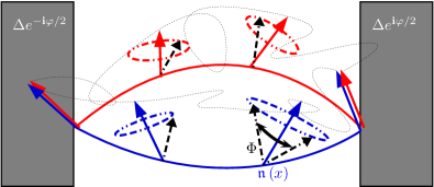
Figure 1: Sketch of the Josephson junction, with $\varphi$ the phase-difference between the two superconducting electrodes (in grey). The white part corresponds to the normal region, with a spin texture giving rise to the Andreev-Wilson loop $W\left(x\right)$ at point $x$, see Eq.(28). The electron spin precesses at a constant latitude around the local vector $\boldsymbol{\mathfrak{n}}$ when travelling along the junction ($\boldsymbol{\mathfrak{n}}$ evolves according to the equation (41)). Blue and red colors refer to a precession axis for electrons and holes, respectively. After completing the loop, the spin rotates an angle $\Phi$ between the initial and final states.

Since $u$ is a SU(2) rotation matrix, so is the operator $W\left(x\right)$ obtained by a combination of rotations. One can thus parameterize the Andreev-Wilson loop operator by a unit vector $\boldsymbol{\mathfrak{n}}$ and an angle $\Phi$ as follows

$$W\left(x\right)=e^{\mathbf{i}\left(\boldsymbol{\mathfrak{n}\cdot\sigma}\right)\Phi}=\cos\Phi+\mathbf{i}\left(\boldsymbol{\mathfrak{n}\cdot\sigma}\right)\sin\Phi\,.$$ (29)

The parameters $\boldsymbol{\mathfrak{n}}$ and $\Phi$ are related to the spin fields $A_{0}$ and $\bm{A}$ via the path-ordered representation, Eq.(20), of the propagators $u$ and $\bar{u}$ in Eq.(28). Importantly, $\boldsymbol{\mathfrak{n}}$ and $\Phi$ encode all physical effects of spin interactions (Zeeman and spin orbit) as the latter enter the Green’s function $g(x)$ only via the Andreev-Wilson loop operator.

By taking a trace of Eqs.(28) and (29) we find that the quantity

$$2\cos\Phi =\operatorname{Tr}\left\{W\left(x\right)\right\}=\operatorname{Tr}\left\{\bar{u}\left(x_{L},x_{R}\right)u\left(x_{R},x_{L}\right)\right\}$$ (30)

appearing in the denominator of (26) is position independent. Therefore the angle $\Phi$ is a $x$-independent global parameter and only $\mathfrak{n}$ may depend on the position $x$ in (29). The unit vector $\boldsymbol{\mathfrak{n}}\left(x\right)$ determines the local spin quantization axis. Semiclassically it can be viewed as an axis about which the spin precesses at a constant latitude. The angle $\Phi$ records the phase accumulated by the electron wave function after one cycle along the Andreev loop (see Fig. 1). This is nothing but the holonomy associated to the equation (19) for $u$ along the Andreev loop. The physical significance of the Andreev-Wilson loop operator is illustrated on Fig.1. When an electron travels from the left to the right electrode inside the normal region, its spin precesses at a constant latitude about a position dependent axis $\boldsymbol{\mathfrak{n}}\left(x\right)$. At the right interface it is converted into a hole according to the scheme of Andreev reflection (Andreev, 1964). The spin of the resulting hole, moving from the right to the left electrode, precesses about the time-reversal conjugate of $\boldsymbol{\mathfrak{n}}$. At the left interface another Andreev reflection transforms the hole back to an electron-like particle with the spin precessing again about the direction of $\boldsymbol{\mathfrak{n}}$. When returning to its original position, the electron spinor accumulates an extra “magnetic” phase $\Phi$ according to the Andreev-Wilson loop operator $W\left(x\right)$ in (29). The phase $\Phi$ is nothing but the angle between the initial and final directions of the electron spin (Konschelle et al., 2016).

By substituting $W(x)$ of Eq.(29) into Eq.(26) and using the trigonometric identity

$$\tan\left(a+b\right)+\tan\left(a-b\right)=\dfrac{2\sin 2a}{\cos 2a+\cos 2b}$$ (31)

we find the following explicit representation for the quasi-classical Green’s function in the normal region $x_{L}\leq x\leq x_{R}$

$$g\left(x\right)=-\dfrac{\mathbf{i}}{2}\sum_{\beta=\pm}\left(1+\beta\boldsymbol{\mathfrak{n}}\left(x\right)\boldsymbol{\cdot\sigma}\right)T_{+\beta}\left(\omega\right)\Theta\left(v_{x}\right)\\ -\dfrac{\mathbf{i}}{2}\sum_{\beta=\pm}\left(1-\beta\boldsymbol{\mathfrak{n}}\left(x\right)\boldsymbol{\cdot\sigma}\right)T_{-\beta}\left(\omega\right)\Theta\left(-v_{x}\right)$$ (32)

$$T_{\alpha\beta}\left(\omega\right)=\tan\left(\frac{\omega L}{\left|v_{x}\right|}+\arcsin\dfrac{\omega}{\Delta}+\alpha\dfrac{\varphi}{2}+\beta\dfrac{\Phi}{2}\right)$$ (33)

The function $T_{\alpha\beta}(\omega)$ in (32) is a constant in space, and represents the spectrum of the electronic states above and below the energy gap. Above the gap, one has to analytically continue the function $\arcsin\left(\omega/\Delta\right)$ such that $g\rightarrow 1$ when $\omega\rightarrow\infty$. This spectral function contains the phase shift $\Phi$ due to the spin precession when the electron and hole propagate along an Andreev loop in the normal region. In addition, the complete spin structure of the Green function appears as the Pauli matrix $\boldsymbol{\mathfrak{n}\cdot\sigma}$ which can be position dependent, as we will explore in section VI.

The electron Green’s function in the superconductors reads

$$g\left(x\geq x_{R}\right)=\dfrac{-\mathbf{i}\omega}{\sqrt{\Delta^{2}-\omega^{2}}}\left(1-e^{-2\frac{x-x_{R}}{|v_{x}|}\sqrt{\Delta^{2}-\omega^{2}}}\right)\\ +e^{-2\frac{x-x_{R}}{|v_{x}|}\sqrt{\Delta^{2}-\omega^{2}}}g\left(x_{R}\right)$$ (34)

$$g\left(x\leq x_{L}\right)=\dfrac{-\mathbf{i}\omega}{\sqrt{\Delta^{2}-\omega^{2}}}\left(1-e^{2\frac{x-x_{L}}{|v_{x}|}\sqrt{\Delta^{2}-\omega^{2}}}\right)\\ +e^{2\frac{x-x_{L}}{|v_{x}|}\sqrt{\Delta^{2}-\omega^{2}}}g\left(x_{L}\right)$$ (35)

with $g\left(x_{L,R}\right)$ given by Eq.(32). As expected physically the spin dependent component of the solution decays exponentially from the S/N interfaces with characteristic length $\hbar v_{F}/\sqrt{\Delta^{2}-\omega^{2}}$ at a given energy, so that $g(x)$ converges to the bulk solution $g_{\infty}=-\mathbf{i}\omega/\sqrt{\Delta^{2}-\omega^{2}}$ when $x\rightarrow\pm\infty$.

Given the electronic Green’s function we can compute the observables (8)-(10). In the normal region one obtains the following final results

$$j_{x}=-e\dfrac{\pi}{2}N_{0}k_{B}T\sum_{n=0}^{\infty}\sum_{\alpha,\beta=\pm}\left\langle\left|v_{x}\right|\alpha T_{\alpha\beta}\left(\mathbf{i}\omega_{n}\right)\right\rangle$$ (36)

$$S^{a}\left(x\right)=-\dfrac{\pi}{2}N_{0}k_{B}T\\ \times\sum_{n=0}^{\infty}\sum_{\alpha,\beta=\pm}\left\langle\operatorname{sgn}\left(v_{x}\right)\mathfrak{n}^{a}\left(x\right)\beta T_{\alpha\beta}\left(\mathbf{i}\omega_{n}\right)\right\rangle$$ (37)

$$\mathfrak{J}_{i}^{a}\left(x\right)=-\dfrac{\pi}{2}N_{0}k_{B}T\\ \times\sum_{n=0}^{\infty}\sum_{\alpha,\beta=\pm}\left\langle v_{i}\operatorname{sgn}\left(v_{x}\right)\mathfrak{n}^{a}\left(x\right)\beta T_{\alpha\beta}\left(\mathbf{i}\omega_{n}\right)\right\rangle$$ (38)

where $T_{\alpha\beta}\left(\omega\right)$ in Eq.(33) is analytically continued to imaginary axis and evaluated at the Matsubara frequencies.

The expressions (36)-(38) represent the central result of the present paper. They are valid for any length, temperature and spin dependent interaction encoded in the definitions of $\Phi$ and $\boldsymbol{\mathfrak{n}}$ in (29). They are also independent of the explicit form of the Fermi surface, which is hidden in the angular averaging $\left\langle\cdots\right\rangle$. In a general case these expressions can only be evaluated numerically. Notice that for a ballistic S/N/S junction, when there is no magnetic interaction in N one simply has $u=\bar{u}=1$ and thus $\Phi=0$, $\boldsymbol{\mathfrak{n}}=\boldsymbol{0}$ and Eq. (36) gives the well known current-phase relation

$$j_{x}^{\text{SNS}}=-eN_{0}k_{B}T\sum_{n=0}^{\infty}\sum_{\alpha=\pm}\times\\ \left\langle\left|v_{x}\right|\alpha\tan\left(\dfrac{\mathbf{i}\omega_{n}L}{\left|v_{x}\right|}+\arcsin\dfrac{\mathbf{i}\omega_{n}}{\Delta}+\alpha\dfrac{\varphi}{2}\right)\right\rangle$$ (39)

which has been studied intensively in the literature, see e.g. (Nazarov, 1994, 1999) and references therein. A finite spin-orbit coupling in the S/N/S does not change the current-phase relation since it will lead to the symmetry $u=\bar{u}$ and hence $W=1$, which implies $\Phi=0$, see (29).

From the equation of motion (19) for the $u$’s and the definition (28) for $W$ one has

$$\mathbf{i}\dfrac{dW}{ds}+\left[A_{0}+\boldsymbol{v\cdot A},W\right]=0$$ (40)

$$\dfrac{d\boldsymbol{\mathfrak{n}}^{a}}{ds}+2\varepsilon^{abc}\left(A_{0}^{b}+v_{i}A_{i}^{b}\right)\boldsymbol{\mathfrak{n}}^{c}=0$$ (41)

where we have used (29) for the second expression. One sees from these equations that the spin quantities (37) and (38) are covariantly conserved $\mathfrak{D}_{0}S+\mathfrak{D}_{i}\mathfrak{J}_{i}=0$ because $\left[A_{0}+\boldsymbol{v\cdot A},\boldsymbol{\mathfrak{n}\cdot\sigma}\right]^{a}=2\mathbf{i}\varepsilon^{abc}\left(A_{0}^{b}+v_{i}A_{i}^{b}\right)\boldsymbol{\mathfrak{n}}^{c}\sigma^{c}$.

According to Eq. (36), the charge current is only odd in phase (it is odd in the sum over $\alpha$), a generic statement from a problem when the $\text{SU}\left(2\right)$ magnetic field is neglected, as discussed in details in (Konschelle et al., 2015). In contrary, the spin-observables (37) and (38) are even in phase (even in the $\alpha$-summation), and so the spin observables may be finite even if the supercurrent is zero and $\varphi=0$.

Simplification of equations (36)-(38) can be readily obtained for the observables for temperatures close to the critical temperature $T_{c}$ (equivalently when $\Delta/k_{B}T_{c}\ll 1$) in the long junction limit $L/\xi_{T}\gg 1$ with the thermal length $\xi_{T}=\hbar v_{F}/2\pi k_{B}T_{c}$

$$\lim_{T\rightarrow T_{c}}j_{x}=-\dfrac{N_{0}}{\pi}e\dfrac{\Delta^{2}}{k_{B}T_{c}}\sin\varphi\\ \times\left\langle e^{-Lv_{F}/\xi_{T}\left|v_{x}\right|}\left|v_{x}\right|\cos\Phi\right\rangle$$ (42)

$$\lim_{T\rightarrow T_{c}}S^{a}=-\dfrac{N_{0}}{\pi}\dfrac{\Delta^{2}}{k_{B}T_{c}}\cos\varphi\\ \times\left\langle e^{-Lv_{F}/\xi_{T}\left|v_{x}\right|}\operatorname{sgn}\left(v_{x}\right)\mathfrak{n}^{a}\sin\Phi\right\rangle$$ (43)

$$\lim_{T\rightarrow T_{c}}\mathfrak{J}_{i}^{a}=-\dfrac{N_{0}}{\pi}\dfrac{\Delta^{2}}{k_{B}T_{c}}\cos\varphi\\ \times\left\langle e^{-Lv_{F}/\xi_{T}\left|v_{x}\right|}v_{i}\operatorname{sgn}\left(v_{x}\right)\mathfrak{n}^{a}\sin\Phi\right\rangle$$ (44)

where $\mathfrak{n}^{a}$ and $\Phi$ contain some angular properties.

Another compact expression for (36) can be obtained in the short-junction limit where contributions of order $\omega L/\left|v_{x}\right|\sim L/\xi_{T}\ll 1$ are neglected (see Appendix B)

$$\lim_{L/\xi_{T}\rightarrow 0}\dfrac{j_{x}}{j_{0}}=\sum_{\alpha=\pm}\left\langle\dfrac{\left|v_{x}\right|}{v_{F}}K_{\alpha}\left(\varphi,\Phi\right)\right\rangle$$ (45)

$$K_{\alpha}=\sin\dfrac{\varphi+\alpha\Phi}{2}\tanh\left(\dfrac{\Delta}{2k_{B}T}\cos\dfrac{\varphi+\alpha\Phi}{2}\right)$$ (46)

where $j_{0}=-e\pi v_{F}N_{0}\Delta/4$. One has to keep in mind that the short junction limit $L\ll\xi_{T}$ has no influence on the ratio between some magnetic length and the length of the junction, so it is justified to keep the full dependency in $\Phi\sim L/\ell_{\text{pr}}$ (for instance the precession length $\ell_{\text{pr}}=2h/\hbar v_{F}$ for a monodomain ferromagnet with exchange field $h$ (Buzdin et al., 1982)). The current-phase expression (45) generalizes well known expressions for the supercurrent in ballistic systems, in all dimensions (see e.g. (Konschelle et al., 2008) and references therein for the S/F/S case). The expressions for the spin observables (38) and (37) become in the limit $L\ll\xi_{T}$:

$$\lim_{L/\xi_{T}\rightarrow 0}\dfrac{S^{a}}{S_{0}}=\sum_{\alpha=\pm}\left\langle\alpha\operatorname{sgn}\left(v_{x}\right)\mathfrak{n}^{a}K_{\alpha}\right\rangle$$ (47)

$$\lim_{L/\xi_{T}\rightarrow 0}\dfrac{\mathfrak{J}_{i}^{a}}{S_{0}}=\sum_{\alpha=\pm}\left\langle\alpha v_{i}\operatorname{sgn}\left(v_{x}\right)\mathfrak{n}^{a}K_{\alpha}\right\rangle$$ (48)

with $S_{0}=-\pi N_{0}\Delta/4$.

Finally, in the long junction limit one has (see Appendix B)

$$\lim_{L/\xi_{T}\rightarrow\infty}j_{x}=-e\dfrac{\pi}{2}N_{0}k_{B}T\left\langle\dfrac{\left|v_{x}\right|\cos\Phi}{\sinh\dfrac{\pi TL}{\left|v_{x}\right|}}\right\rangle\sin\varphi$$ (49)

$$\lim_{L/\xi_{T}\rightarrow\infty}S^{a}=-\dfrac{\pi}{2}N_{0}k_{B}T\left\langle\dfrac{\operatorname{sgn}\left(v_{x}\right)\mathfrak{n}^{a}\left(x\right)\sin\Phi}{\sinh\dfrac{\pi TL}{\left|v_{x}\right|}}\right\rangle\cos\varphi$$ (50)

$$\lim_{L/\xi_{T}\rightarrow\infty}\mathfrak{J}_{i}^{a}=-\dfrac{\pi}{2}N_{0}k_{B}T\left\langle\dfrac{v_{i}\operatorname{sgn}\left(v_{x}\right)\mathfrak{n}^{a}\left(x\right)\sin\Phi}{\sinh\dfrac{\pi TL}{\left|v_{x}\right|}}\right\rangle\cos\varphi\;.$$ (51)

In the rest of this work we analyze the physical consequences of the above general solution for the ballistic S/N/S Josephson junction with generic spin-dependent fields. In particular we explore the behavior of the spin-resolved density of states, the distribution of the spin polarization, the spin and the charge currents for various configurations of the spin fields.

IV Density of states

Let us start from the analysis of the density of states in the N bridge, in particular its dependence on the magnetic phase shift $\Phi$.

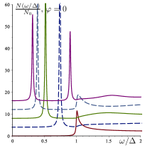
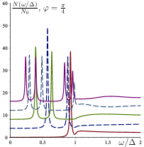
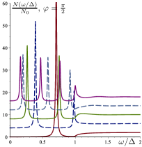
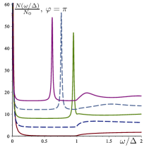
Figure 2: Density of state with respect to the energy $\omega/\Delta$ from the expression (54) for $\Phi=0$. In each panel different lengths of the junction are represented: $L/\xi_{0}=\left\{0,1,2,3,4\right\}$ ($\xi_{0}=\hbar v_{F}/\Delta$ is the coherence length), with a constant offset of each curve from the previous one for commodity, and an alternance of plain and dashed curves. Top-left panel: $\varphi=0$, top-right panel: $\varphi=\pi/4$, bottom-left panel: $\varphi=\pi/2$, bottom-right panel: $\varphi=\pi$. One sees that increasing the length of the junction allows the opening of new Andreev modes, which eventually goes to zero energy when $\varphi$ approach $\pi$. Longer and longer junctions allow for more and more Andreev modes to appear.

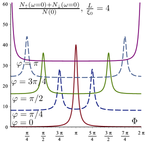
Figure 3: Density of state at zero energy from the expression (54) with respect to $\Phi$. Different phase-difference of the junction are represented: $\varphi=\left\{0,1,2,3,4\right\}\times\pi/4$, with a constant offset of each curve from the previous one for commodity, and an alternance of plain and dashed curves. The plot is for $L/\xi_{0}=4$, but any length displays the same zero-energy peaks, namely when $\Phi\pm\varphi=\pi$, generally broader for longer junctions. Note that the possible length-dependency of the parameter $\Phi$ has not been taken into account for this check.

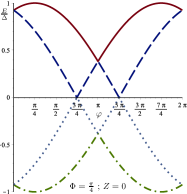
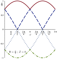
Figure 4: Energy $E\left(\varphi\right)/\Delta$ of the Andreev bound states with respect to the phase difference $\varphi$ for a short junction $L/\xi_{0}\rightarrow 0$, from the expression (56). $\Phi=\pi/4$ (left panel), and $\Phi=\pi/2$ (right panel). At the value $\varphi=\pi$ and $\varphi=\pi\pm\Phi$, the curves are spin degenerate in the upper or lower half planes.

From the expression for the Green’s function (32), one sees that the local matrix structure $\boldsymbol{\mathfrak{n}\cdot\sigma}$ can be diagonalized at any given point $x$. The quantities

$$g_{\uparrow}(\omega)=-\dfrac{\mathbf{i}}{2}\left(T_{++}\left(\omega\right)\Theta\left(v_{x}\right)+T_{-+}\left(\omega\right)\Theta\left(-v_{x}\right)\right)$$ (52)

and

$$g_{\downarrow}(\omega)=-\dfrac{\mathbf{i}}{2}\left(T_{+-}\left(\omega\right)\Theta\left(v_{x}\right)+T_{--}\left(\omega\right)\Theta\left(-v_{x}\right)\right)$$ (53)

represent Green’s functions for the spin up and down with respect to the local axis $\boldsymbol{\mathfrak{n}}(x)$ , with the function $T_{\alpha\beta}(\text{$\omega$)}$ defined in Eq. (33). Then the density of states (DOS) per unit energy and per unit spin is calculated as follows

$$\dfrac{N_{\uparrow,\downarrow}\left(\omega\right)}{N\left(0\right)}=\lim_{\epsilon\rightarrow 0}\dfrac{\Re\left\langle g_{\uparrow,\downarrow}\left(\omega+\mathbf{i}\epsilon\right)\right\rangle}{\pi}$$ (54)

The total DOS is given by $N_{\uparrow}+N_{\downarrow}$ whereas the spectral spin density will be proportional to $N_{\uparrow}-N_{\downarrow}$. These two quantities can be in principle measured by spin-polarized near-field spectroscopy.

The DOS is plotted on Fig.2 for different ratios of $L/\xi_{0}$ with $\xi_{0}=\hbar v_{F}/\Delta$ the coherence length, and for several values of $\varphi$ at $\Phi=0$. The increase of the junction length leads to an increase of the number of Andreev channels. A zero energy peaks in the DOS appear for $\varphi\approx\pi$.

When $\Phi\neq 0$, a peak at zero-energy can be generated each time $\Phi\pm\varphi=\pi$. For instance when $\varphi=\pi/4$, a zero-energy peak appears for $\Phi=3\pi/4$ and for $\Phi=5\pi/4$. The spectral weight of the Andreev channels depend on the precise value of the total phase ($\varphi\pm\Phi$ plus the length contribution $\omega L/v_{F}$) accumulated along the junction, and the zero-energy peaks tend to decrease and become broader for longer junction, see Fig.3. Importantly, the zero-energy peak seems to be a generic feature of the presence of magnetic interaction in the ballistic bridge. Zero bias peaks were also obtained in diffusive Josephson systems (Jacobsen et al., 2015; Arjoranta and Heikkilä, 2016) or in S/F/F systems (Alidoust et al., 2015).

The Andreev bound-states are now routinely measured in state-of-the-art experiments (Lee et al., 2012; Bretheau et al., 2013). They are obtained from the poles of the denominator in Eq.(54). Specifically the energies $E_{\alpha,\beta}$ with $\alpha,\beta=\left\{\pm\right\}$ of the bound states verify the following quasi-classic quantization condition

$$\dfrac{E_{\alpha,\beta}L}{v_{x}}-\arccos\dfrac{E_{\alpha,\beta}}{\Delta}+\alpha\dfrac{\varphi}{2}+\beta\dfrac{\Phi}{2}=n\pi\;;\;n\in\mathbb{Z}\;.$$ (55)

The two bound states characterized by the energy $E_{\alpha+}$ and $E_{\alpha-}$ correspond to the spin degree of freedom, and so a spin-resolved spectroscopy of the Andreev bound states with respect to the phase at a given length and temperature ($\Delta$ fixed) would determine $\Phi$. The bound states are double degenerate when $\Phi=2n\pi$, $\forall n\in\mathbb{Z}$ ; in these cases the quantization condition (55) has been first established by Kulik in the pure semi-classic limit, i.e. when $E/\Delta\rightarrow 0$ and so $\arccos\left(E/\Delta\right)\rightarrow\pi/2$, the Maslov index being $1/2$ in this case (Kulik, 1970; Duncan and Györffy, 2002).

When $L/\xi_{0}=0$, there are four branches with expressions

$$\dfrac{E_{\sigma}\left(\varphi\right)}{\Delta}=\pm\sqrt{\cos^{2}\dfrac{\varphi+\sigma\Phi}{2}}$$ (56)

as plotted in Fig.4. They are at least double degenerate at the value $E_{\alpha\pm}=0$ when $\varphi=\pm\Phi$. When $\Phi=0$ or $\Phi=\pi$, the two curves in the upper half-plane are spin degenerate, as well as the two curves in the lower half-plane. Similar result has been obtained in (Fogelstrom, 2000; Barash and Bobkova, 2002), eventually generalized to the case of a point-contact with spin-active interfaces. One sees that the zero-energy DOS obtained in Fig.3 are in fact associated to the anti-crossing of the Andreev bound states (at least in the short-junction limit).

We should emphasize that the zero-energy Andreev states obtained here are a generic consequence of proximity effect under spin interactions and that they also exist for finite transparency, as shown in our previous work (Konschelle et al., 2016). These zero energy states are not related to zero-energy Majorana modes, which are absent of our analysis. Our zero-energy crossings do not describe any topological phase transition since they occur only at certain values of the spin-splitting field encoded in $\Phi$.

V Magnetic Moment in a S/F/S Junction

In this section we calculate the spin polarization of conduction electrons in a S/F/S structure in the simplest non-trivial situation with $\Phi\neq 0$ and a constant vector $\boldsymbol{\mathfrak{n}}$. This is, nevertheless, a generalization of the results for the magnetic moment induced in S/F bilayers studied in earlier works (Bergeret et al., 2004a; Krivoruchko and Koshina, 2002; Bergeret et al., 2004b; Bergeret and García, 2004; Bergeret et al., 2005a, b; Kharitonov et al., 2006; Xia et al., 2009). The case of a Bloch domain wall, which implies a position dependent $\boldsymbol{\mathfrak{n}}$, will be discussed in section VII.

For definiteness, we choose $\boldsymbol{\mathfrak{n}}\left(x\right)=\boldsymbol{\hat{z}}$, the unit vector along the $z$-axis. This situation corresponds to a variable exchange-field directed along the $z$-axis only $A_{0}=h\left(x\right)\sigma_{z}/\hbar$, but with arbitrary spatial dependence. In this case $\Phi=2\int_{-L/2}^{L/2}h\left(x\right)dx/v_{x}$ is the exchange field integrated over the junction. When $h$ is constant along the junction, then $\Phi=2hL/v_{x}$ and we recover the usual oscillations of the critical current with respect to the length and/or exchange field of the junction (Buzdin, 2005; Bergeret et al., 2005a; Konschelle et al., 2008). For an anti-ferromagnetic ordering, say for example two equal domains with up and down magnetization, $\Phi=0$ and there is no signature of the magnetic proximity effect, as has been obtained after a long calculation in (Blanter and Hekking, 2004). In contrast, our method provides a simple and clear way to understand this issue immediately.

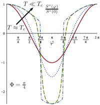
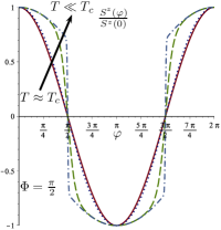
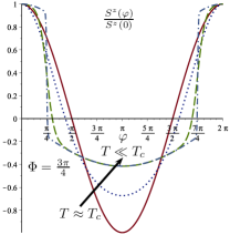
Figure 5: Spin-polarization $S^{z}\left(\varphi\right)/S^{z}\left(0\right)$ in 1D monodomain S/F/S Josephson-junction from Eq.(59) with respect to the phase-difference $\varphi$ and for different values of the temperature $t=T/T_{c}=0.99$ (plain/red), $0.5$ (blue/dotted), $0.1$ (green/dashed) and $0.01$ (blue/dotted-dashed) showing steeper and steeper curves as the temperature is decreased. Left panel: $\Phi=2hL/v_{F}=\pi/4$. Middle panel: $\Phi=\pi/2$. Right panel: $\Phi=3\pi/4$.

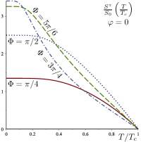
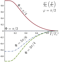
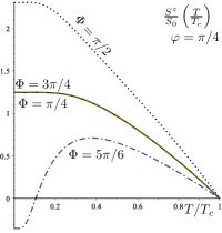
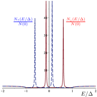
Figure 6: Spin-polarization $S^{z}$ in 1D monodomain S/F/S Josephson-junction from Eq.(59) with respect to the temperature $T/T_{c}$ for different values of $\Phi=2hL/v_{F}=\pi/4$ (red/plain), $\pi/2$ (blue/dotted), $3\pi/4$ (green/dashed), $5\pi/6$ (blue/dotted-dashed), at zero-phase-difference $\varphi=0$ (upper left panel), $\pi/2$ (upper right panel) and $\pi/4$ (lower left panel). The diamagnetic magnetization saturates at low temperatures and vanishes for $T\rightarrow T_{c}$. A reversal of the spin polarization is predicted in the bottom panel. This is understood when plotting the density of state for $\varphi=\pi/4$ and $\Phi=5\pi/6$ (lower right panel), when one superimposes a Fermi distribution law, since the heights of the different peaks are similar.

The charge current (36) in the junction reduces in this case to the form

$$j_{x}^{\text{SFS}}=-e\dfrac{\pi}{2}N_{0}k_{B}T\sum_{n=0}^{\infty}\sum_{\alpha,\beta=\pm}\times\\ \left\langle\left|v_{x}\right|\alpha\tan\left(\dfrac{\mathbf{i}\omega_{n}L}{\left|v_{x}\right|}+\arcsin\dfrac{\mathbf{i}\omega_{n}}{\Delta}+\alpha\dfrac{\varphi}{2}+\beta\dfrac{\Phi}{2}\right)\right\rangle$$ (57)

Such a current-phase relation has been thoroughly investigated in the past, see e.g. (Buzdin, 2005; Bergeret et al., 2005a; Golubov et al., 2004; Konschelle et al., 2008)

In addition to the charge current, an S/F/S junction is expected to host a finite spin polarization, which can be calculated from Eq.(37). When $A_{0}=h\left(x\right)\sigma_{z}/\hbar$, only $S^{z}$ survives, and we get

$$S^{z}=-\dfrac{\pi}{2}N_{0}k_{B}T\sum_{n=0}^{\infty}\sum_{\alpha,\beta=\pm}\left\langle\operatorname{sgn}\left(v_{x}\right)\beta T_{\alpha\beta}\left(\mathbf{i}\omega_{n}\right)\right\rangle$$ (58)

for arbitrary length or

$$\lim_{L\ll\xi_{T}}\dfrac{S^{z}}{S_{0}}=\sum_{\alpha=\pm}\left\langle\alpha\operatorname{sgn}\left(v_{x}\right)K_{\alpha}\right\rangle$$ (59)

in the short-junction limit, with $T_{\alpha\beta}$ given in Eq. (33) and $K_{\alpha}$ in (46). Since we are considering a constant $\boldsymbol{\mathfrak{n}}$, the spin-polarization is position independent inside the bridge and vanishes for $\Phi=\left\{0,\pi\right\}$.

We show in Fig.5 the spin-polarization in a short 1D junction ($v_{x}=\pm v_{F}$) versus the phase difference $\varphi$ and in Fig.6 as a function of the temperature $T/T_{c}$. For the computation we use the interpolation formula $\Delta\left(T\right)\approx 1.764T_{c}\tanh\left(1.74\sqrt{T_{c}/T-1}\right)$ for the superconducting gap.

It is clear from Fig.6 that the induced correction to the spin-polarization is a consequence of the proximity effect and vanishes at temperatures larger than the critical temperature. For certain values of $\varphi$ and $\Phi$ the spin-polarization can change its sign as a function of temperature, as shown, for example, in the right panel of Fig.6 for $\Phi=5\pi/6$ and $\varphi=\pi/4$. This behavior can be explained by the thermal occupancy of the Andreev levels induced in the F region. In Fig.6 we show the spin polarized density of state (DOS) for $\Phi=5\pi/6$ and $\varphi=\pi/4$. One sees that the peaks in the DOS for up and down electrons have different height. The spin-polarization is obtained by multiplying the DOS by the occupancy of the levels, i.e the equilibrium Fermi distribution function, and integrating over energies. At low temperatures the dominant peak is the left-most one, which is $\uparrow$-spin polarized, resulting in a negative spin polarization. However for higher enough temperatures, the higher peak being $\downarrow$-polarized starts to become more populated, and at $T\rightarrow T_{c}$ its height dominates over the $\uparrow$-peak, i.e. the surface under the Fermi distribution favors the $\downarrow$-polarization, then making an overall spin polarization of positive sign.

VI Spin polarization and spin currents in junctions with spin-orbit coupling

In this section we discuss the spin dependent effects in a junction with both spin-splitting and spin-orbit effects. We calculate the spin density and the spin current in the normal region of the junction. Experimental interests in these quantities grew up recently (Wakamura et al., 2014, 2015).

To remain on analytically accessible ground, we consider the situations when both $A_{0}$ and $\boldsymbol{v\cdot A}$ are position independent. In that case, we can integrate (19) exactly. Firstly, due to the translational invariance in the N-region the spin propagators depend only on the difference of coordinates: $u\left(s_{2},s_{1}\right)=u\left(s_{1}-s_{2}\right)$ and the spin propagator reduces to a simple exponential,

$$u\left(s\right)=e^{\mathbf{i}\left(A_{0}+\boldsymbol{v\cdot A}\right)s}\equiv\exp\left[\mathbf{i}\left(A_{0}^{a}+v^{j}A_{j}^{a}\right)\sigma^{a}s\right].$$

Therefore the general expression of Eq.(28) for the Andreew-Wilson loop operator simplifies as follows

$$W(x)=e^{\frac{\mathbf{i}}{v_{x}}\left(A_{0}+\boldsymbol{v\cdot A}\right)\left(x+L/2\right)}\\ \times e^{\frac{\mathbf{i}}{v_{x}}\left(A_{0}-\boldsymbol{v\cdot A}\right)L}e^{\frac{\mathbf{i}}{v_{x}}\left(A_{0}+\boldsymbol{v\cdot A}\right)\left(L/2-x\right)}\;.$$ (60)

It is important to notice that $W$ is a covariant object since it determines all observables. In particular $W$ can be written in terms of the SU(2) electric field $F_{0k}=-\mathbf{i}\left[A_{0},A_{k}\right]$ and combinations of its covariant derivatives $\mathfrak{D}_{k}F_{0j}=-\mathbf{i}\left[A_{k},F_{0j}\right]$. To simplify further the discussion, we focus on the $T\rightarrow T_{c}$ limits of the spin density (43) and spin current (44). We also restrict the analysis to the 1D and 2D situations, which are relevant experimentally. We thus consider only Rashba ($A_{x}^{y}=-A_{y}^{x}$) or Dresselhaus ($A_{x}^{x}=-A_{y}^{y}$) cases. According to (43) and (44) the spin density and spin current are determined by $\boldsymbol{\mathfrak{n}}\left(x\right)\sin\Phi$ which is the spin non-trivial part of $W$. By performing an expansion of (60) with respect to $LA_{i}/v_{x}$ one can show that the spin density reads:

$$S=-\dfrac{N_{0}}{\pi}\dfrac{\Delta^{2}}{k_{B}T_{c}}\cos\varphi\left\langle e^{-Lv_{F}/\xi_{T}\left|v_{x}\right|}\operatorname{sgn}\left(v_{x}\right)\left[\frac{2L}{v_{x}}A_{0}+\frac{2xL}{v_{x}^{2}}v_{k}F_{0k}-\frac{4L^{3}}{3v_{x}^{3}}A_{0}^{3}-\dfrac{L}{v_{x}^{3}}v_{j}\mathfrak{D}_{j}F_{0k}v_{k}\left(\frac{L^{2}}{12}+x^{2}\right)+\cdots\right]\right\rangle$$ (61)

whereas the spin current takes the form

$$\mathfrak{J}_{i}=-\dfrac{N_{0}}{\pi}\dfrac{\Delta^{2}}{k_{B}T_{c}}\cos\varphi\left\langle e^{-Lv_{F}/\xi_{T}\left|v_{x}\right|}v_{i}\operatorname{sgn}\left(v_{x}\right)\left[\left(\dfrac{L}{v_{x}^{3}}\mathfrak{D}_{0}F_{0k}v_{k}-\dfrac{2}{3}\dfrac{xL}{v_{x}^{4}}\mathfrak{D}_{0}v_{j}\mathfrak{D}_{j}F_{0k}v_{k}\right)\left(\frac{L^{2}}{4}-x^{2}\right)+\cdots\right]\right\rangle$$ (62)

We now discuss the physical meaning of (61) and (62). For a short enough junction, the surviving term is the $S\propto A_{0}L$, which is nothing but the polarization caused by the spin-splitting field in S/F/S system, see section V.

In addition to the S/F/S phenomenology, there are extra phenomenologies mixing spin-orbit and spin-splitting effects, all proportional to the electric field $F_{0k}v_{k}$. For instance the second order term is proportional to the electric field $xLF_{0x}$ (after angular averaging, only $F_{0x}$ survives). In addition it is odd in space, therefore the spin density will present different signs at the two interfaces. Thus the term $S\propto xLF_{0x}$ can be seen as the analog to the capacitor effect in electrostatics, here in a S/N/S junction: the existence of a finite electric field in the N region separates “charges” which in this case translate into spin densities with different signs. In other words, in the S/N/S structure the accumulation of charge corresponds to an accumulation of the spin polarization at the boundaries between the normal and the superconducting regions. For this reason we denote this effect the spin capacitor effect. It is illustrated on Fig.7 for a 2D Rashba system.

The spin current has in the leading order a contribution of the type (see Eq.(62)) : $\mathfrak{J}_{i}\sim\left(L^{2}/4-x^{2}\right)\mathfrak{D}_{0}F_{0i}$ (angular averaging evaluated). This resembles the expression for the displacements currents in electrostatics as the time derivative of the electric field, and one calls them the displacement spin currents. For either a Rashba or a Dresselhaus coupling, there are potentially two components of the electric field $F_{0x}\propto\left[A_{0},A_{x}\right]$ and $F_{0y}\propto\left[A_{0},A_{y}\right]$. Each of these allow for a displacement current along the junction or perpendicular to it, see Fig.7 for an illustration of $\mathfrak{J}_{x}^{y}$ and $\mathfrak{J}_{y}^{x}$ in the case of Rashba coupling, when $A_{0}^{z}$, $A_{x}^{y}$ and $A_{y}^{x}$ are present.

At first sight one may think that the spin density and spin currents may obey equations equivalent to those in electrostatics. However this is not always true. Higher order terms in Eq. (62) clearly show that the expressions for the spin density and spin current also contains higher order covariant derivatives of the electric field that eventually leads to creation of other components of both quantities as discussed below. For instance the fourth order term in the expansion Eq. (62) after angular averaging for a 2D gas reads

$$\mathfrak{J}_{x}^{\left(4\right)} \propto\mathfrak{D}_{0}\left(2\mathfrak{D}_{x}F_{x0}+\mathfrak{D}_{y}F_{y0}\right)$$

$$\mathfrak{J}_{y}^{\left(4\right)} \propto\mathfrak{D}_{0}\left(\mathfrak{D}_{y}F_{x0}+\mathfrak{D}_{x}F_{y0}\right)\;.$$ (63)

In the case of Rashba SOC when the Zeeman term points toward the $x$-axis, the only surviving term is $\mathfrak{J}_{y}^{\left(4\right)}\propto\mathfrak{D}_{0}\mathfrak{D}_{y}F_{x0}\rightarrow\mathfrak{J}_{y}^{z}$. When the Zeeman effect is present through $A_{0}^{y}$ only, $\mathfrak{J}_{y}^{\left(4\right)}\propto\mathfrak{D}_{0}\mathfrak{D}_{x}F_{y0}$ and there are two contributions $\mathfrak{J}_{y}^{z}$ and $\mathfrak{J}_{y}^{x}$. These situations are illustrated on Fig.8 which, as discussed below, is obtained form the exact expression. The component of the spin current $\mathfrak{J}_{y}^{x}$ in the upper panel of this figure would require even higher order terms in the expansion (62).

We now go beyond the above expansion and write explicitly $W$ by combining Eq. (60) with the representation Eq.(29). In particular we obtain the following equations which determine the local spin quantization axis $\boldsymbol{\mathfrak{n}}\left(x\right)$ and the magnetic phase shift $\Phi$

$$\cos\Phi=\cos\dfrac{\kappa_{+}L}{v_{x}}\cos\dfrac{\kappa_{-}L}{v_{x}}\\ -\dfrac{\boldsymbol{\kappa_{+}\cdot\kappa_{-}}}{\kappa_{+}\kappa_{-}}\sin\dfrac{\kappa_{+}L}{v_{x}}\sin\dfrac{\kappa_{-}L}{v_{x}}\;,$$ (64)

$$\boldsymbol{\mathfrak{n}}\left(x\right)\sin\Phi=-\dfrac{\boldsymbol{\kappa_{+}}}{\kappa_{+}}\left(\sin\dfrac{\kappa_{+}L}{v_{x}}\cos\dfrac{\kappa_{-}L}{v_{x}}+\dfrac{\boldsymbol{\kappa_{+}\cdot\kappa_{-}}}{\kappa_{+}\kappa_{-}}\cos\dfrac{\kappa_{+}L}{v_{x}}\sin\dfrac{\kappa_{-}L}{v_{x}}\right)\\ +\left[\left(\dfrac{\boldsymbol{\kappa_{+}}}{\kappa_{+}}\dfrac{\boldsymbol{\kappa_{+}\cdot\kappa_{-}}}{\kappa_{+}\kappa_{-}}-\dfrac{\boldsymbol{\kappa_{-}}}{\kappa_{-}}\right)\cos\dfrac{2\kappa_{+}x}{v_{x}}-\dfrac{\boldsymbol{\kappa_{+}\times\kappa_{-}}}{\kappa_{+}\kappa_{-}}\sin\dfrac{2\kappa_{+}x}{v_{x}}\right]\sin\dfrac{\kappa_{-}L}{v_{x}}$$ (65)

where $\boldsymbol{\kappa_{\pm}}$ are the vectors with the components

$$\kappa_{\pm}^{a}=A_{0}^{a}\pm\sum_{i=1}^{3}v_{i}A_{i}^{a}$$ (66)

and the norm $\kappa_{\pm}=\sqrt{\boldsymbol{\kappa_{\pm}\cdot\kappa_{\pm}}}$. In the special case when $\boldsymbol{\kappa_{+}}=\boldsymbol{\kappa_{-}}=\boldsymbol{\kappa}$ we get $\Phi=2\kappa L/v_{x}$ and $\boldsymbol{\mathfrak{n}}\left(x\right)=\boldsymbol{\kappa}/\kappa$ (a constant), which corresponds to a pure exchange field, $A_{0}\neq 0$ and $A_{i}^{a}=0$, discussed in Sec.V. A generic situation will exhibit a space dependent precession axis $\boldsymbol{\mathfrak{n}}\left(x\right)$, as can be seen from the second line of Eq.(65). In particular, the function $\boldsymbol{\mathfrak{n}}(x)$ has both odd and even contributions with respect to the center of the junction. Notice that both the components of $S$ and the current can be explained for this particular case in terms of the spin capacitor effect and displacement currents.

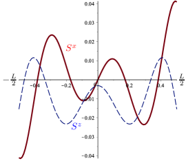
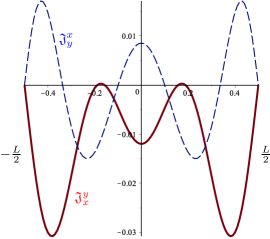
Figure 7: The upper panel shows the spatial dependence of the spin polarizations $S^{x}$ (plain curve) and $S^{z}$ (dashed curve) for a Rashba SOC and an exchange field in $z$-direction. Lower panel shows the spatial dependence of the spin currents $\mathfrak{J}_{x}^{y}$ (plain curve) and $\mathfrak{J}_{y}^{x}$ (dotted curve) in the same situation. with $\mathfrak{J}_{i}\propto\mathfrak{D}_{0}F_{0i}$ in analogy with a displacement current, see (62). The spin capacitor effect is illustrated by the $S^{x}$ curve, being odd in space and originating from the term $S\propto\mathfrak{D}_{i}F_{i0}$ in (61). We have chosen $\boldsymbol{h}=\left(0,0,5\right)\hbar v_{F}/\xi_{T}$, $\xi_{T}r=3$, $L/\xi_{T}=1$, and the curves are normalized by the quantity $2N_{0}\Delta^{2}\cos\varphi/\pi k_{B}T_{c}$. For a Dresselhaus SOC ($\gamma=\pi/2$), one obtains similar curves by making the changes $S^{x}\rightarrow-S^{y}$, $S^{z}\rightarrow S^{z}$, $\mathfrak{J}_{x}^{y}\rightarrow\mathfrak{J}_{x}^{x}$ and $\mathfrak{J}_{y}^{x}\rightarrow\mathfrak{J}_{y}^{y}$.

We now focus on the Rashba and Dresselhaus SOC that we parametrize using two parameters $r$ and $\gamma$. The Rashba coupling enters as $A_{x}^{y}=-A_{y}^{x}=r\cos\gamma$ whereas the Dresselhaus coupling reads $A_{x}^{x}=-A_{y}^{y}=r\sin\gamma$. In addition to the spin-orbit couplings we assume a spin-splitting field parameterized by the coordinates $h_{x,y,z}$ . One then obtains

$$\boldsymbol{\kappa_{\pm}}=\left(\begin{array}[]{c}h_{x}\mp v_{F}r\sin\left(\phi-\gamma\right)\\ h_{y}\pm v_{F}r\cos\left(\phi+\gamma\right)\\ h_{z}\end{array}\right)$$ (67)

for a circular Fermi level parameterized by $\boldsymbol{v}=v_{F}\left(\cos\phi,\sin\phi\right)$ in a 2D system. We substitute this $\boldsymbol{\kappa}_{\pm}$ in (65) in order to evaluate the spin polarizations (43) and the spin currents (44) close to the critical temperature. Fig.7 shows the result for a Rashba spin-orbit coupling, i.e. $\gamma=0$ in (67). If one chooses a Dresselhaus coupling instead (with $\gamma=\pi/2$), the curves are similar, except $S^{y}\left(\gamma=\pi/2\right)=-S^{x}\left(\gamma=0\right)$, $S^{z}\left(\pi/2\right)=S^{z}\left(0\right)$, $\mathfrak{J}_{x}^{x}\left(\pi/2\right)=\mathfrak{J}_{x}^{y}\left(0\right)$, $\mathfrak{J}_{y}^{y}\left(\pi/2\right)=\mathfrak{J}_{y}^{x}\left(0\right)$, all the other spin observables being zero when $h_{x}=h_{y}=0$. For this reason we do not show the case of a Dresselhaus coupling.

As expected from our previous perturbative analysis the spin density has in both cases two contributions: the one due to the Zeeman polarization, $S^{z}$ and those due to the capacitor effect, $S^{{}^{x}}$ for Rashba and $S^{y}$ for Dresselhaus. Other contributions parallel to the field component $F_{0y}$ vanish due to the velocity average (cf. Eq. 61). Also in Fig.7 the currents can be explained from the lowest term in the expansion Eq.(62) as displacement currents induced by electric field component $F_{0x}$, $\mathfrak{J}_{x}^{y}$ for the Rashba case and $\mathfrak{J}_{y}^{y}$ in the Dresselhaus SOC. There are also displacements currents induced by $F_{0y}$ component of the field which are $\mathfrak{J}_{y}^{x}$ in the Rashba case (see Fig. 7 bottom panel) and $\mathfrak{J}_{y}^{y}$ in the Dresselhaus case (not shown).

All the previous spin densities and currents can be explained again in terms of the spin capacitor effect and displacement currents, and their symmetry with respect to $x$ is determined by the leading terms in the expansions Eqs.(61)-(62). When the spin-splitting field is applied in $x$ or $y$ direction also higher order terms in Eq. (62) contribute to the spin currents and generates additional components. As an example we show the transverse currents for different directions of $A_{0}$ in Fig. 8.

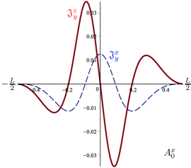
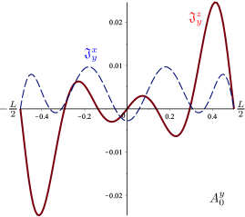
Figure 8: Illustration of the transverse spin current $\mathfrak{J}_{y}^{z,x}$ (plain/dashed curves respectively) along the axis perpendicular to the junction for a Rashba spin-orbit effect with respect to the junction length. We choose $L/\xi_{T}=1$, $\xi_{T}r=3$, $\xi_{T}h_{x}=5\hbar v_{F}$ (upper panel) and $\xi_{T}h_{y}=5\hbar v_{F}$ (lower panel) in Eqs.(43)-(44) after injection of $\boldsymbol{\mathfrak{n}}$ from (65) and (67). The antisymmetric $\mathfrak{J}_{y}^{z}$ comes from the contribution $\left\langle v_{i}\operatorname{sgn}\left(v_{x}\right)\mathfrak{D}_{0}v_{j}\mathfrak{D}_{j}F_{0k}v_{k}\right\rangle$ in (62). The vertical axis is in unit of $2N_{0}\Delta^{2}\cos\varphi/\pi k_{B}T_{c}$. When $h_{x}=h_{y}=0$ but $h_{z}\neq 0$ this term is zero, and no asymmetric spin current is flowing, see Fig.7. The current $\mathfrak{J}_{y}^{x}$ stems for higher order terms in the expansion (62).

VII Non-homogenoues exchange field

Figure 9: Magnetic interaction $\cos\Phi$ for a Bloch domain wall with respect to the parameter $hL/\left|v_{x}\right|$, from (70), and for different values of $\kappa=v_{x}q/2h$. Plain line: $\kappa=0$. Dotted line $\kappa=1.5$. Dashed line $\kappa=3$.

For completeness in this section we briefly discuss the effect of a inhomogeneous magnetization. In particular we consider a Bloch domain wall, characterized by a $x$-dependent exchange field

$$A_{0}=h\left[\sigma^{2}\sin qx+\sigma^{3}\cos qx\right]$$ (68)

which could be included in (19) in order to obtain $u\left(x\right)$. Nevertheless, one can take advantage of the gauge-covariant formalism, and show that the Bloch domain wall is in fact gauge-equivalent to a situation with a constant exchange field $A_{0}^{z}=h$ in addition to a spin-orbit interaction $A_{x}^{x}=-q/2$ (Bergeret and Tokatly, 2014), for which (19) reduces to

$$\mathbf{i}\dfrac{du}{ds}+\left(h\sigma^{3}-v_{x}\dfrac{q}{2}\sigma^{1}\right)u\left(s\right)=0$$ (69)

and can be easily integrated. Since $\Phi$ is gauge-invariant, one has

$$\cos\Phi=\cos^{2}\left(\sqrt{1+\kappa^{2}}\dfrac{hL}{v_{x}}\right)-\\ -\dfrac{1-\kappa^{2}}{1+\kappa^{2}}\sin^{2}\left(\sqrt{1+\kappa^{2}}\dfrac{hL}{v_{x}}\right)$$ (70)

from (64), with $\kappa=v_{x}q/2h$. Expression (70) is plotted on Fig.9. For a monodomain, $\kappa\rightarrow 0$ and $\Phi\rightarrow 2hL/v_{x}$, as usual for a S/F/S junction, see section V. For larger $\kappa$, $\Phi$ takes only limited values (see Fig.9), and for $\kappa\rightarrow\infty$ one has $\Phi\rightarrow 0$, recovering a pure S/N system. This later situation corresponds to the situation described in section V, when the alternance of domains with opposite spin orientations reduces the characteristic oscillations of the S/F proximity effect, eventually destroying these oscillations in ballistic systems when the magnetization averaged along the junction vanishes. Since the domain wave-length $q=-2A_{x}^{x}$ is equivalent to a spin-orbit effect, a large $\kappa$ is equivalent to a large spin-orbit effect, or equivalently a vanishing exchange field.

In a junction with a Bloch domain wall, there are the generation of spin current polarized along the junction axis, as can be drawn from the conclusions of section VI when $A_{0}^{z}$ and $A_{x}^{x}$ are present. In the lowest order in the fields, the spin capacitor effect is present with a contribution $S^{y}\propto\partial_{x}F_{0x}^{y}$ odd in space, and the displacement spin current $\mathfrak{J}_{x}^{x}\propto\left(\mathfrak{D}_{0}F_{0x}\right)^{x}\propto A_{0}^{z}F_{0x}^{y}\left[\sigma^{z},\sigma^{y}\right]$ shows up.

VIII Conclusion

Ballistic S/N/S Josephson systems when the normal region N exhibits generic spin-dependent fields have been investigated. We propose a systematic approach to study systems exhibiting both spin-splitting and spin-orbit interactions, provided the latter is linear-in-momentum and the magnetic interaction is weak, such that the quasi-classical approximation is valid (section II).

We have shown that the magnetic interactions appears in all observables as a global phase accumulation $\Phi$ (see (30)) and a space dependent unit vector $\boldsymbol{\mathfrak{n}}$ (see (29)). With the help of the derived compact expression for the quasi-classic Green’s function, Eq.(32), we studied different spin-dependent fields and their effects on the properties of the junction.

In particular we have demonstrated that the density of states may show a zero-energy peak which is a generic consequence of a finite $\Phi$.

We have also shown how such fields in the N region generate finite changes of the spin-polarization and finite spin currents. We identify the possibility for the accumulation of the spin at the interfaces between the normal and superconducting regions, an effect reminiscent to the charge accumulation at the plates of a capacitor. Hence we call this phenomenon the spin capacitor effect. In addition, we predict the generation of spin currents flowing along the superconducting interfaces. Both these effects can be understood in a convenient way using an $\text{SU}\left(2\right)$ electrostatics, which generalizes the Maxwell electrostatics to the non-Abelian case.

Effects like the spin capacitor, or the predicted spectral features can be experimentally verified in superconducting heterostructures which are being fabricated in the present, and attract more and more interest recently. The measurement of the spin polarization and charge current can serve as a powerful characterization of the symmetries of the spin texture. The tunability of the superconducting condensate via voltage or current bias allow for a coherent manipulation of the spin polarization and currents. Reciprocally, the manipulation of the spin quantities allow for the manipulation of the superconducting coherent states. Research along these lines are promising in addition to the search for topological effects in spin textured superconducting systems.

Appendix A Green’s functions

We fix positive velocities in this appendix. Let us write (24) in its explicit form

$$\left(\begin{array}[]{cc}Q_{11}&Q_{12}\\ Q_{21}&Q_{22}\end{array}\right)\left(\begin{array}[]{cc}-1&g_{1}\\ 0&1\end{array}\right)=\left(\begin{array}[]{cc}-1&0\\ g_{2}&1\end{array}\right)\left(\begin{array}[]{cc}Q_{11}&Q_{12}\\ Q_{21}&Q_{22}\end{array}\right)$$ (71)

in the Nambu space, where the quantities $Q_{ij}$ are matrices in the spin space, as well as the $g_{1,2}$, and can be easilly obtained from the definition (25). Component by component, one gets

$$Q_{11} =Q_{11}$$

$$Q_{11}g_{1}+Q_{12} =-Q_{12}$$

$$-Q_{21} =g_{2}Q_{11}+Q_{21}$$

$$Q_{21}g_{1}+Q_{22} =g_{2}Q_{12}+Q_{22}$$ (72)

and one sees that the solutions of the two intermediary equations $g_{1}=-2Q_{11}^{-1}Q_{12}$ and $g_{2}=-2Q_{21}Q_{11}^{-1}$ automatically verifies the last one, which can be thought as a consistency equation. To get $g_{1}$ or $g_{2}$, we now want to invert $Q_{11}$, which is a $2\times 2$ matrix. Defining

$$\tilde{\chi}=\arcsin\dfrac{\omega}{\Delta}+\dfrac{\varphi}{2}+\omega\left(s_{R}-s_{L}\right)$$ (73)

one has

$$2Q_{11}\cos\arcsin\dfrac{\omega}{\Delta}=e^{\mathbf{i}\tilde{\chi}}u\left(s_{R},s_{L}\right)+e^{-\mathbf{i}\tilde{\chi}}\bar{u}\left(s_{R},s_{L}\right)$$ (74)

for the matrix $Q_{11}$ defined in (25). The inverse $Q_{11}^{-1}$ is obtained using the property

$$\left(e^{\mathbf{i}\tilde{\chi}}u\left(s_{R},s_{L}\right)+e^{-\mathbf{i}\tilde{\chi}}\bar{u}\left(s_{R},s_{L}\right)\right)\left(e^{\mathbf{i}\tilde{\chi}}u\left(s_{L},s_{R}\right)+e^{-\mathbf{i}\tilde{\chi}}\bar{u}\left(s_{L},s_{R}\right)\right)=2\cos 2\tilde{\chi}+\operatorname{Tr}\left\{u\left(s_{R},s_{L}\right)\bar{u}\left(s_{L},s_{R}\right)\right\}$$ (75)

since the $u$’s are $2\times 2$ unitary matrices and thus reads $u=\dfrac{1}{\sqrt{\left|\alpha\right|^{2}+\left|\beta\right|^{2}}}\left(\begin{array}[]{cc}\alpha&\beta\\ -\beta^{\ast}&\alpha^{\ast}\end{array}\right)$ for $\alpha,\;\beta\in\mathbb{C}$. They thus verify $u+u^{\dagger}=\mathbb{I}\operatorname{Tr}\left\{u\right\}$ with $\mathbb{I}$ the identity matrix. It is clear that $u\left(s_{R},s_{L}\right)\bar{u}\left(s_{L},s_{R}\right)$ is unitary as well. One has thus

$$Q_{11}^{-1}=\left(e^{\mathbf{i}\tilde{\chi}}u\left(s_{L},s_{R}\right)+e^{-\mathbf{i}\tilde{\chi}}\bar{u}\left(s_{L},s_{R}\right)\right)\dfrac{2\cos\arcsin\dfrac{\omega}{\Delta}}{2\cos 2\tilde{\chi}+\operatorname{Tr}\left\{u\left(s_{R},s_{L}\right)\bar{u}\left(s_{L},s_{R}\right)\right\}}$$ (76)

and finally one obtains

$$g_{1}=2\mathbf{i}\dfrac{e^{-\mathbf{i}\arcsin\frac{\omega}{\Delta}}\bar{u}\left(s_{L},s_{R}\right)u\left(s_{R},s_{L}\right)-e^{\mathbf{i}\arcsin\frac{\omega}{\Delta}}u\left(s_{L},s_{R}\right)\bar{u}\left(s_{R},s_{L}\right)+2\mathbf{i}\sin\left(2\omega\left(s_{R}-s_{L}\right)+\varphi+\arcsin\dfrac{\omega}{\Delta}\right)}{2\cos\left(2\omega\left(s_{R}-s_{L}\right)+\varphi+2\arcsin\dfrac{\omega}{\Delta}\right)+\operatorname{Tr}\left\{u\left(s_{R},s_{L}\right)\bar{u}\left(s_{L},s_{R}\right)\right\}}$$ (77)

$$g_{2}=-2\mathbf{i}\dfrac{e^{-\mathbf{i}\arcsin\frac{\omega}{\Delta}}u\left(s_{R},s_{L}\right)\bar{u}\left(s_{L},s_{R}\right)-e^{\mathbf{i}\arcsin\frac{\omega}{\Delta}}\bar{u}\left(s_{R},s_{L}\right)u\left(s_{L},s_{R}\right)+2\mathbf{i}\sin\left(2\omega\left(s_{R}-s_{L}\right)+\varphi+\arcsin\dfrac{\omega}{\Delta}\right)}{2\cos\left(2\omega\left(s_{R}-s_{L}\right)+\varphi+2\arcsin\dfrac{\omega}{\Delta}\right)+\operatorname{Tr}\left\{u\left(s_{R},s_{L}\right)\bar{u}\left(s_{L},s_{R}\right)\right\}}$$ (78)

then $g\left(s_{0}\right)$ is obtained as (26) for $v_{x}>0$, after injection of $g_{1}$ or $g_{2}$ in (23). One gets

$$2g\left(s_{0}\right)\cos\arcsin\dfrac{\omega}{\Delta}=-2\mathbf{i}\sin\arcsin\dfrac{\omega}{\Delta}+\mathbf{i}u\left(s_{0},s_{L}\right)g_{1}u\left(s_{L},s_{0}\right)$$ (79)

for the particle component (i.e. the component $11$ of the $\check{g}$ matrix) of eq.(23) and one evaluates

$$g\left(s_{0}\right)=\dfrac{u\left(s_{0},s_{R}\right)\bar{u}\left(s_{R},s_{L}\right)u\left(s_{L},s_{0}\right)-u\left(s_{0},s_{L}\right)\bar{u}\left(s_{L},s_{R}\right)u\left(s_{R},s_{0}\right)-2\mathbf{i}\sin\left(2\omega\left(s_{R}-s_{L}\right)+\varphi+\arcsin\dfrac{\omega}{\Delta}\right)}{2\cos\left(2\omega\left(s_{R}-s_{L}\right)+\varphi+\arcsin\dfrac{\omega}{\Delta}\right)+\operatorname{Tr}\left\{u\left(s_{R},s_{L}\right)\bar{u}\left(s_{L},s_{R}\right)\right\}}$$ (80)

straightforwardly. The case $v_{x}<0$ is obtained by the solutions in the superconducting electrodes

$$\check{g}\left(s\leq s_{L}\right) =e^{\mathbf{i}\tau_{3}\varphi/4}\dfrac{e^{\mathbf{i}\eta/2}-\mathbf{i}\tau_{1}e^{\mathbf{i}\eta/2}}{\sqrt{2\cos\eta}}e^{-\tau_{3}\Delta\left(s-s_{L}\right)\tau_{3}\cos\eta}\left[g_{3}\tau_{-}-\tau_{3}\right]e^{\tau_{3}\Delta\left(s-s_{L}\right)\tau_{3}\cos\eta}\dfrac{e^{\mathbf{i}\eta/2}+\mathbf{i}\tau_{1}e^{-\mathbf{i}\eta/2}}{\sqrt{2\cos\eta}}e^{\mathbf{i}\tau_{3}\varphi/4}$$

$$\check{g}\left(s\geq s_{R}\right) =e^{-\mathbf{i}\tau_{3}\varphi/4}\dfrac{e^{\mathbf{i}\eta/2}-\mathbf{i}\tau_{1}e^{\mathbf{i}\eta/2}}{\sqrt{2\cos\eta}}e^{-\tau_{3}\Delta\left(s-s_{R}\right)\tau_{3}\cos\eta}\left[g_{4}\tau_{+}-\tau_{3}\right]e^{\tau_{3}\Delta\left(s-s_{L}\right)\tau_{3}\cos\eta}\dfrac{e^{\mathbf{i}\eta/2}+\mathbf{i}\tau_{1}e^{-\mathbf{i}\eta/2}}{\sqrt{2\cos\eta}}e^{-\mathbf{i}\tau_{3}\varphi/4}$$ (81)

instead of (23). It gives $\mathbf{Q}^{-1}\left[g_{4}\tau_{+}-\tau_{3}\right]=\left[g_{3}\tau_{-}-\tau_{3}\right]\mathbf{Q}^{-1}$ instead of (24), with $\mathbf{Q}^{-1}\left(\varphi,s_{L},s_{R}\right)=\mathbf{Q}\left(-\varphi,s_{R},s_{L}\right)$. One has thus $g_{4,3}\left(\varphi,s_{L},s_{R}\right)=g_{1,2}\left(-\varphi,s_{R},s_{L}\right)$. Since $s=x/v_{x}$ one has, $s_{R}-s_{L}=L/v_{x}$ when $v_{x}>0$ and $s_{L}-s_{R}=L/\left|v_{x}\right|$ for $v_{x}<0$ when choosing $s_{R,L}=\pm L/v_{x}$. One finally obtains (26) independent of the sign of the velocity.

The $f_{0}$ matrix reads (we do not use this expression here, but it is required to calculate perturbations, see e.g. (Konschelle et al., 2015))

$$f\left(s\right)=-2\mathbf{i}\dfrac{e^{-2\mathbf{i}\omega\left(s_{L}-s\right)}e^{\mathbf{i}\frac{\varphi}{2}}e^{\mathbf{i}\arcsin\frac{\omega}{\Delta}}u\left(s,s_{R}\right)\bar{u}\left(s_{R},s\right)+e^{-2\mathbf{i}\omega\left(s_{R}-s\right)}e^{-\mathbf{i}\frac{\varphi}{2}}e^{-\mathbf{i}\arcsin\frac{\omega}{\Delta}}u\left(s,s_{L}\right)\bar{u}\left(s_{L},s\right)}{2\cos\left(2\omega\left(s_{R}-s_{L}\right)+\varphi+2\arcsin\dfrac{\omega}{\Delta}\right)+\operatorname{Tr}\left\{u\left(s_{R},s_{L}\right)\bar{u}\left(s_{L},s_{R}\right)\right\}}$$ (82)

at the point $s\in\left[s_{L},s_{R}\right]$. Eq.(82) is given for positive velocity only $v_{x}>0$. The contribution $v_{x}<0$ is obtained by the substitution $\left(\varphi,s_{L},s_{R}\right)\rightarrow\left(-\varphi,s_{R},s_{L}\right)$ as before. One can calculate $\bar{f}\left(s\right)=\mathcal{T}f\left(s\right)\mathcal{T}^{-1}$ and $\bar{g}=\mathcal{T}g\mathcal{T}^{-1}$, the time-reversals of $f$ and $g$, and then verify that $\check{g}^{2}=1$ straightforwardly.

Appendix B Short and long junction limits

To understand how to get the short junction limit (45), one writes

$$\sum_{\alpha,\beta=\pm}\alpha T_{\alpha\beta}\left(\omega\right)\\ =\sum_{\alpha,\beta=\pm}\tan\left(\dfrac{\varphi+\alpha\Phi}{2}+\beta\dfrac{\omega L}{\left|v_{x}\right|}+\beta\arcsin\dfrac{\omega}{\Delta}\right)\\ =\sum_{\alpha=\pm}\dfrac{2\sin\left(\varphi+\alpha\Phi\right)}{\cos\left(\varphi+\alpha\Phi\right)+\cos 2\left(\dfrac{\omega L}{\left|v_{x}\right|}+\arcsin\dfrac{\omega}{\Delta}\right)}$$ (83)

with $T_{\alpha\beta}$ in (33), and playing with the parity of the tangent, the sums over $\alpha$ and $\beta$ and finally using the formula (31) in order to isolate the terms in $\omega$.

The short junction verifies $\omega L/v_{F}\propto L/\xi_{T}\ll 1$ and so one gets

$$\lim_{L/\xi_{T}\ll 1}\sum_{\alpha,\beta=\pm}\alpha T_{\alpha\beta}=\sum_{\alpha=\pm}\dfrac{2\sin\left(\varphi+\alpha\Phi\right)}{2\cos^{2}\dfrac{\varphi+\alpha\tau}{2}-\dfrac{\omega^{2}}{\Delta^{2}}}$$ (84)

which can be converted to Matsubara frequencies $\omega=\mathbf{i}\omega_{n}=\mathbf{i}\pi k_{B}T\left(2n+1\right)$ and then sum over $n$. One obtains

$$\sum_{n\geq 0}\lim_{L/\xi_{T}\ll 1}\sum_{\alpha,\beta=\pm}\alpha T_{\alpha\beta}=\\ \sum_{\alpha=\pm}\dfrac{\Delta}{2k_{B}T}\sin\dfrac{\varphi+\alpha\Phi}{2}\tanh\left(\dfrac{\Delta}{2k_{B}T}\cos\dfrac{\varphi+\alpha\Phi}{2}\right)$$ (85)

using usual tricks to evaluate the sum

$$\sum_{n=0}^{\infty}\dfrac{1}{\alpha^{2}+\beta^{2}\left(n+1/2\right)^{2}}=\dfrac{\pi}{2\alpha\beta}\tanh\dfrac{\pi\alpha}{\beta}\;;\;\alpha,\beta\in\mathbb{R}$$ (86)

see e.g. (Mahan, 2000). This is directly proportional to (the sum over $\alpha$ of) $K_{\alpha}$ in (46).

For the spin observables, one uses the following tricks

$$\sum_{\alpha,\beta=\pm}\beta T_{\alpha\beta}\left(\omega\right)\\ =\sum_{\alpha,\beta=\pm}\tan\left(\dfrac{\alpha\varphi+\Phi}{2}+\beta\dfrac{\omega L}{\left|v_{x}\right|}+\beta\arcsin\dfrac{\omega}{\Delta}\right)\\ =\sum_{\alpha,\beta=\pm}\alpha\tan\left(\dfrac{\varphi+\alpha\Phi}{2}+\beta\dfrac{\omega L}{\left|v_{x}\right|}+\beta\arcsin\dfrac{\omega}{\Delta}\right)$$ (87)

and so the sum is now odd in $\alpha$, which subsists in the expressions for the spin density (47) and the spin current (48) in the short junction limit. The sum over the Matsubara frequencies is the same as before and can be performed irrespective of the presence of $\alpha$, hence one gets $\sum_{\alpha}\alpha K_{\alpha}$ in (47) and (48).

In the long junction limit, one starts again with either (83) or (87) but we apply this time $\omega L/v_{F}\propto L/\xi_{T}\gg 1$ such that

$$\lim_{L/\xi_{T}\gg 1}\sum_{\alpha,\beta=\pm}\alpha T_{\alpha\beta}=\sum_{\alpha=\pm}\dfrac{2\sin\left(\varphi+\alpha\Phi\right)}{\cos\left(\varphi+\alpha\Phi\right)+\cos\dfrac{2\omega L}{\left|v_{x}\right|}}$$ (88)

from (83). Thus we have

$$\lim_{L/\xi_{T}\gg 1}\sum_{\alpha,\beta=\pm}\alpha T_{\alpha\beta}=2\sin\varphi\cos\Phi e^{-2\omega_{n}L/\left|v_{x}\right|}$$ (89)

and so

$$\sum_{n\geq 0}\lim_{L/\xi_{T}\gg 1}\sum_{\alpha,\beta=\pm}\alpha T_{\alpha\beta}=\dfrac{\sin\varphi\cos\Phi}{\sinh\dfrac{\pi TL}{\left|v_{x}\right|}}$$ (90)

$$\sum_{n\geq 0}\lim_{L/\xi_{T}\gg 1}\sum_{\alpha,\beta=\pm}\beta T_{\alpha\beta}=\dfrac{\cos\varphi\sin\Phi}{\sinh\dfrac{\pi TL}{\left|v_{x}\right|}}$$ (91)

since the sum over the Matsubara frequencies can be performed easily

$$\sum_{n=0}^{\infty}e^{-\alpha\left(n+1/2\right)}=\dfrac{1}{2\sinh\dfrac{\alpha}{2}}\;;\;\alpha\in\mathbb{R}_{+}$$ (92)

as a geometric progression. In the long junction limit, the trajectories $v_{x}$ with large angles from the junction axis are killed exponentially (say the trajectories $v_{x}=v_{F}\cos\phi$ with $\phi\approx\pi/2$ for a circular Fermi surface) and do not participate to the transport. In the long junction limit, the Andreev bound states are equally spaced, and we recover the effective action of a harmonic oscillator.

References

- Eschrig (2011) M. Eschrig, Physics Today 64, 43 (2011).
- Linder and Robinson (2015) J. Linder and J. W. A. Robinson, Nature Physics 11, 307 (2015), arXiv:1510.00713 .
- Eschrig (2015) M. Eschrig, Reports on Progress in Physics 78, 104501 (2015), arXiv:1509.02242 .
- Xiang et al. (2012) Z.-L. Xiang, S. Ashhab, J. Q. You, and F. Nori, Reviews of Modern Physics 85, 35 (2012), arXiv:1204.2137 .
- Nayak et al. (2008) C. Nayak, A. Stern, M. H. Freedman, and S. Das Sarma, Reviews of Modern Physics 80, 1083 (2008), arXiv:0707.1889 .
- Alicea and Stern (2014) J. Alicea and A. Stern, (2014), arXiv:1410.0359 .
- Casalbuoni and Nardulli (2004) R. Casalbuoni and G. Nardulli, Reviews of Modern Physics 76, 263 (2004), arXiv:0305069 [hep-ph] .
- Buzdin (2005) A. I. Buzdin, Reviews of Modern Physics 77, 935 (2005).
- Bergeret et al. (2005a) F. S. Bergeret, A. F. Volkov, and K. B. Efetov, Reviews of Modern Physics 77, 1321 (2005a).
- Robinson et al. (2010) J. W. A. Robinson, J. D. S. Witt, and M. G. Blamire, Science (New York, N.Y.) 329, 59 (2010).
- Khaire et al. (2010) T. S. Khaire, M. A. Khasawneh, W. P. Pratt, and N. O. Birge, Physical Review Letters 104, 137002 (2010), arXiv:0912.0205 .
- Anwar et al. (2010) M. Anwar, F. Czeschka, M. Hesselberth, M. Porcu, and J. Aarts, Physical Review B 82, 100501 (2010).
- Anwar et al. (2012) M. S. Anwar, M. Veldhorst, A. Brinkman, and J. Aarts, Applied Physics Letters 100, 052602 (2012), arXiv:1111.5809 .
- Visani et al. (2012) C. Visani, Z. Sefrioui, J. Tornos, C. Leon, J. Briatico, M. Bibes, A. Barthélémy, J. Santamaría, and J. E. Villegas, Nature Physics 8, 539 (2012).
- Khaydukov et al. (2014) Y. N. Khaydukov, G. A. Ovsyannikov, A. E. Sheyerman, K. Y. Constantinian, L. Mustafa, T. Keller, M. A. Uribe-Laverde, Y. V. Kislinskii, A. V. Shadrin, A. Kalaboukhov, B. Keimer, and D. Winkler, Physical Review B 90, 035130 (2014), arXiv:1406.5442 .
- Singh et al. (2015) A. Singh, S. Voltan, K. Lahabi, and J. Aarts, Physical Review X 5, 021019 (2015), arXiv:1410.4973 .
- Kalcheim et al. (2015) Y. Kalcheim, O. Millo, A. Di Bernardo, A. Pal, and J. W. A. Robinson, , 1 (2015), arXiv:1508.01070 .
- Wakamura et al. (2014) T. Wakamura, N. Hasegawa, K. Ohnishi, Y. Niimi, and Y. Otani, Physical Review Letters 112, 036602 (2014).
- Wakamura et al. (2015) T. Wakamura, H. Akaike, Y. Omori, Y. Niimi, S. Takahashi, A. Fujimaki, S. Maekawa, and Y. Otani, Nature Materials , 1 (2015).
- Mal’shukov and Chu (2008) A. Mal’shukov and C. Chu, Physical Review B 78, 104503 (2008), arXiv:0801.4419 .
- Mal’shukov et al. (2010) A. G. Mal’shukov, S. Sadjina, and A. Brataas, Physical Review B 81, 060502 (2010).
- Alidoust and Halterman (2015a) M. Alidoust and K. Halterman, New Journal of Physics 17, 033001 (2015a), arXiv:1504.05950 .
- Alidoust and Halterman (2015b) M. Alidoust and K. Halterman, Journal of Physics: Condensed Matter 27, 235301 (2015b), arXiv:1502.05719 .
- Konschelle et al. (2015) F. Konschelle, I. V. Tokatly, and F. S. Bergeret, Physical Review B 92, 125443 (2015), arXiv:1506.02977 .
- Konschelle and Buzdin (2009) F. Konschelle and A. I. Buzdin, Physical Review Letters 102, 017001 (2009), arXiv:0810.4286 .
- Kulagina and Linder (2014) I. Kulagina and J. Linder, Physical Review B 90, 054504 (2014), arXiv:1406.7016 .
- Bergeret and Tokatly (2015) F. S. Bergeret and I. V. Tokatly, Europhysics Letters (EPL) 110, 57005 (2015), arXiv:1409.4563 .
- Eilenberger (1968) G. Eilenberger, Zeitschrift für Physik 214, 195 (1968).
- Larkin and Ovchinnikov (1969) A. I. Larkin and Y. N. Ovchinnikov, Sov. Phys. JETP 28, 1200 (1969).
- Bergeret and Tokatly (2014) F. S. Bergeret and I. V. Tokatly, Physical Review B 89, 134517 (2014), arXiv:1402.1025 .
- Konschelle (2014) F. Konschelle, The European Physical Journal B 87, 119 (2014), arXiv:1403.1797 .
- Bergeret and Tokatly (2013) F. S. Bergeret and I. V. Tokatly, Physical Review Letters 110, 117003 (2013), arXiv:1211.3084 .
- Konschelle et al. (2016) F. Konschelle, F. S. Bergeret, and I. V. Tokatly, Physical Review Letters 116, 237002 (2016), arXiv:1601.02973 .
- Fröhlich and Studer (1992) J. Fröhlich and U. M. Studer, Communications in Mathematical Physics 148, 553 (1992).
- Fröhlich and Studer (1993) J. Fröhlich and U. Studer, Reviews of Modern Physics 65, 733 (1993).
- Berche and Medina (2013) B. Berche and E. Medina, European Journal of Physics 34, 161 (2013), arXiv:1210.0105 .
- Tokatly (2008) I. V. Tokatly, Physical Review Letters 101, 106601 (2008), arXiv:0802.1350 .
- Serene and Rainer (1983) J. Serene and D. Rainer, Physics Reports 101, 221 (1983).
- Rammer and Smith (1986) J. Rammer and H. Smith, Reviews of Modern Physics 58, 323 (1986).
- Langenberg and Larkin (1986) D. N. Langenberg and A. I. Larkin, Nonequilibrium superconductivity (North-Holland, Amsterdam, 1986).
- Wilhelm et al. (1999) F. K. Wilhelm, W. Belzig, C. Bruder, G. Schön, and A. D. Zaikin, Superlattices and Microstructures 25, 1251 (1999), arXiv:9812297 [cond-mat] .
- Kopnin (2001) N. B. Kopnin, Theory of nonequilibrium superconductivity (Oxford {U}niversity {P}ress, Oxford, 2001).
- Bergeret et al. (2004a) F. S. Bergeret, A. F. Volkov, and K. B. Efetov, Physical Review B 69, 174504 (2004a), arXiv:0307468 [cond-mat] .
- Martin-Rodero et al. (1993) A. Martin-Rodero, F. J. Garcia-Vidal, and A. Levy Yeyati, Physical Review Letters 72, 4 (1993), arXiv:9312081 [cond-mat] .
- Sols and Ferrer (1994) F. Sols and J. Ferrer, Physical Review B 49, 15913 (1994), arXiv:9312005 [cond-mat] .
- Levy Yeyati et al. (1995) A. Levy Yeyati, A. Martín-Rodero, and F. J. García-Vidal, Physical Review B 51, 3743 (1995), arXiv:9407089 [cond-mat] .
- Riedel et al. (1996) R. Riedel, L.-F. Chang, and P. Bagwell, Physical Review B 54, 16082 (1996).
- Schopohl and Maki (1995) N. Schopohl and K. Maki, Physical Review B 52, 490 (1995).
- Schopohl (1998) N. Schopohl, (1998), arXiv:9804064 [cond-mat] .
- Blanes et al. (2009) S. Blanes, F. Casas, J. Oteo, and J. Ros, Physics Reports 470, 151 (2009), arXiv:0810.5488 .
- Kulik (1970) I. O. Kulik, Soviet Physics JETP 30, 944 (1970).
- Andreev (1964) A. F. Andreev, Sov. Phys. JETP 19, 1228 (1964).
- Nazarov (1994) Y. V. Nazarov, Physical Review Letters 73, 1420 (1994).
- Nazarov (1999) Y. V. Nazarov, Superlattices and Microstructures 25, 1221 (1999), arXiv:arxiv:9811155 .
- Buzdin et al. (1982) A. I. Buzdin, L. Bulaevskii, and S. V. Panyukov, Sov. Phys. JETP 35, 178 (1982).
- Konschelle et al. (2008) F. Konschelle, J. Cayssol, and A. I. Buzdin, Physical Review B 78, 134505 (2008), arXiv:0807.2560 .
- Jacobsen et al. (2015) S. H. Jacobsen, J. A. Ouassou, and J. Linder, Physical Review B 92, 024510 (2015), arXiv:1503.06835 .
- Arjoranta and Heikkilä (2016) J. Arjoranta and T. T. Heikkilä, Physical Review B 93, 024522 (2016), arXiv:1507.02320 .
- Alidoust et al. (2015) M. Alidoust, K. Halterman, and O. T. Valls, Physical Review B 92, 014508 (2015), arXiv:1506.05469 .
- Lee et al. (2012) E. J. H. Lee, X. Jiang, R. Aguado, G. Katsaros, C. M. Lieber, and S. De Franceschi, Physical Review Letters 109, 186802 (2012), arXiv:1207.1259 .
- Bretheau et al. (2013) L. Bretheau, Ç. Ö. Girit, H. Pothier, D. Esteve, and C. Urbina, Nature 499, 312 (2013).
- Duncan and Györffy (2002) K. Duncan and B. Györffy, Annals of Physics 298, 273 (2002).
- Fogelstrom (2000) M. Fogelstrom, Physical Review B 62, 8 (2000), arXiv:0008074 [cond-mat] .
- Barash and Bobkova (2002) Y. Barash and I. Bobkova, Physical Review B 65, 144502 (2002).
- Krivoruchko and Koshina (2002) V. N. Krivoruchko and E. A. Koshina, Physical Review B 66, 014521 (2002), arXiv:0201534 [cond-mat] .
- Bergeret et al. (2004b) F. S. Bergeret, A. F. Volkov, and K. B. Efetov, Europhysics Letters (EPL) 66, 111 (2004b), arXiv:0403658 [cond-mat] .
- Bergeret and García (2004) F. S. Bergeret and N. García, Physical Review B 70, 052507 (2004), arXiv:0408273 [cond-mat] .
- Bergeret et al. (2005b) F. S. Bergeret, A. L. Yeyati, and A. Martín-Rodero, Physical Review B 72, 064524 (2005b), arXiv:0507334 [cond-mat] .
- Kharitonov et al. (2006) M. Y. Kharitonov, A. F. Volkov, and K. B. Efetov, Physical Review B 73, 054511 (2006), arXiv:0601443 [cond-mat] .
- Xia et al. (2009) J. Xia, V. Shelukhin, M. Karpovski, A. Kapitulnik, and A. Palevski, Physical Review Letters 102, 087004 (2009), arXiv:0810.2605 .
- Blanter and Hekking (2004) Y. M. Blanter and F. W. J. Hekking, Physical Review B 69, 024525 (2004), arXiv:0306706 [cond-mat] .
- Golubov et al. (2004) A. Golubov, M. Kupriyanov, and E. Il’ichev, Reviews of Modern Physics 76, 411 (2004).
- Mahan (2000) G. D. Mahan, Many-particle physics, third edit ed., edited by N. Y. Kluwer Academic / Plenum Publisher (2000).