The distance and luminosity probability distributions derived from parallax and flux with their measurement errors

We use a Bayesian approach to derive the distance probability distribution for one object from its parallax with measurement uncertainty for two spatial distribution priors, viz. a homogeneous spherical distribution and a galactocentric distribution – applicable for radio pulsars – observed from Earth. We investigate the dependence on measurement uncertainty, and show that a parallax measurement can underestimate or overestimate the actual distance, depending on the spatial distribution prior. We derive the probability distributions for distance and luminosity combined, and for each separately, when a flux with measurement error for the object is also available, and demonstrate the necessity of and dependence on the luminosity function prior. We apply this to estimate the distance and the radio and gamma-ray luminosities of PSR J0218+4232. The use of realistic priors improves the quality of the estimates for distance and luminosity, compared to those based on measurement only. Use of a wrong prior, for example a homogeneous spatial distribution without upper bound, may lead to very wrong results.

1 Introduction

Distance determinations are fundamental in astronomy. The study of spatial distributions and source number densities is the most direct application. Together with proper motion measurements, distances form the basis of velocity measurements and kinematic studies. Combined with flux measurements they provide luminosities.

A standard method of distance determination is the measurement of the trigonometric parallax. The conversion of the measured parallax into the most probable actual parallax is not straightforward, as is evident from the excellent historical survey given by Sandage & Saha (2002). Most of the papers discussed in that survey use parallax and apparent magnitude measurements to derive absolute magnitude distributions, or statistical corrections between apparent and absolute magnitudes. In a much cited paper, Lutz & Kelker (1973) derive the probability distribution of the real parallax as a function of the measured parallax and its measurement error. Since that paper, there has been some debate as to whether or not their equation is applicable when only one object is observed (as reviewed by Sandage & Saha 2002).

In a study of radio pulsars, Faucher-Giguère & Kaspi (2006) give a probability distribution of actual distances as a function of the measured parallax, reproduced as Eq.21 below. In an important paper Verbiest et al. (2012) develop a Bayesian method to combine various distance-related measurements and their uncertainties to find the probability distribution of distances, and show the importance of the choice of priors. Verbiest & Lorimer (2014) apply this method in a study of the gamma-ray luminosity of the millisecond pulsar PSR J0218+4232. Alas, they make the same error as Faucher-Giguère & Kaspi (2006) in deriving the probability distribution of actual distances as a function of the measured parallax, and make a similar error in the equation for the probability distribution of luminosity as a function of measured flux and parallax.

Much of the confusion in the existing literature arises because of the failure to dicriminate between what technically are called the frequentist approach and the Bayesian approach, leading to the incorrect conclusion that a measurement by itself provides a probability density distribution centered on the measured value. We briefly explain this error in Sect.1.1, where we also discuss the related confusion on whether population priors must be taken into account in the study of single objects. In contrast to statements in several previous papers (e.g. Feast 2002, Francis 2012, and references therein), the answer is yes if a probability density is required. A more detailed explanation is given in Sect.3. In that Section we repeat some results by Bailer-Jones (2015) that appeared as we were finalizing our paper, but we differ in that we use a spatial distribution appropriate for pulsars.

The structure of our paper is as follows. In Sect.2 we describe the spatial distributions and the luminosity distributions that we use, and explain our notation. In Section 3 we describe in some detail the derivation of the correct conversion of measured parallax to probability distribution of actual distances, for the case of a known (or assumed) distribution in space. We consider a homogeneous distribution, and a galactocentric distribution observed from Earth. The latter is applied to the case of PSR J0218+4232. In Sect.4, we consider objects for which both parallax and flux are measured to determine the probability distributions for distance and luminosity, and illustrate our results for PSR J0218+4232. The gamma-ray luminosity of PSR J0218+4232 is discussed in Sect.5. Finally, in Section 6 we briefly discuss the assumptions that we have made, and the expected consequences of relaxing these.

1.1 Confidence intervals and probability densities

Consider an object whose parallax is measured with accuracy $\sigma$, i.e. the measured value $\varpi^{\prime}$ is a draw from a gaussian centered on its real parallax $\varpi_{1}$ with standard deviation $\sigma$. The probability that a draw leads to a measured value $\varpi^{\prime}$ such that $|\varpi^{\prime}-\varpi_{1}|<\sigma$ is then (roughly) 68%, which corresponds to a 68% probability that the real value $\varpi_{1}$ is in the range given by $\varpi^{\prime}-\sigma<\varpi_{1}<\varpi^{\prime}+\sigma$. Similarly, if the real parallax is $\varpi_{2}$ there is a 68% probability that the real value $\varpi_{2}$ is in the range given by $\varpi^{\prime}-\sigma<\varpi_{2}<\varpi^{\prime}+\sigma$, and so for every real distance $\varpi_{i}$. Thus, no matter what the real distance is, we can state that there is a 68% probability that it is in the range bounded by $\varpi^{\prime}-\sigma$ and $\varpi^{\prime}+\sigma$. Analogously, for each frequency of occurrence, e.g. expressed in percentage $x$%, on may derive the corresponding range: between $\varpi^{\prime}-n_{x}\sigma$ and $\varpi^{\prime}+n_{x}\sigma$, where $n_{x}=1.645$ for 90%, $n_{x}=2$ for 95.5%, etc. Hence the name frequentist approach. The measured value $\varpi^{\prime}$ does not, however, provide the probability distribution within these ranges.

To obtain such a probability distribution one must compute the relative contribution that each possible real parallax $\varpi_{i}$ makes to the probability of measuring $\varpi^{\prime}$, i.e. follow the Bayesian approach. As an illustration, consider a population of 10 sources, 9 of which have $\varpi=5$ mas, and 1 has $\varpi=3$ mas. We select one source from this population for a parallax measurement with accuracy 1 mas, and measure $\varpi^{\prime}=4$ mas. The real parallax answers to the 68% probability of lying within 1 mas of the measured value. A real parallax of 5 mas has a probability of 90%, a real parallax of 3 mas of 10%, and other parallaxes have probability zero. The probability distribution of the real distance $\varpi$ is not given by a gaussian centered on the measured value $\varpi^{\prime}$. Also for the case of a more realistic, continuous intrinsic distribution, the probability distribution of $\varpi$ in general can not be stated to be given by a gaussian centered on the measured value $\varpi^{\prime}$. Therefore, the use of realistic priors improves the quality of the estimate for the distance, compared to that based on one measurement only. The same is true for the estimate of the luminosity.

Finally, consider a series of measurements ${\varpi^{\prime}}_{i}$ made from a single object, each with its own accuracy $\sigma_{i}$. Each measurement is a draw from a distribution centered on the actual distance of the object. The best estimate of $\varpi^{\prime}$, and its accuracy $\sigma$ can be determined by averaging these measurements with appropriate weighting of the individual measurements, without reference to the population priors. The resulting values $\varpi^{\prime}$ and $\sigma$ are the best estimate of the parallax measurement and its error. They may be used in a frequentist approach to determine a confidence interval. To determine a probability density, they must be combined with a population prior.

2 Ingredients and notation

The analysis in this paper is based on measurements of parallax and flux, combined with an intrinsic spatial distribution, which is assumed to be known, and an intrinsic luminosity distribution, also assumed known. The measurement errors lead to probability distributions for measured values that we denote with $g_{D}$ and $g_{S}$ for parallax and flux, respectively. The intrinsic spatial and luminosity distributions are denoted with $f_{D}$ and $f_{L}$, respectively. To illustrate the general methods, we discuss two spatial distributions and two luminosity distributions.

2.1 Measurements

A parallax measurement is subject to measurement error $\sigma$. The measurement error distribution $g_{D}(\varpi^{\prime}|D)$ gives the probability of measuring a parallax $\varpi^{\prime}$ when the actual distance is $D$. $g_{D}(\varpi^{\prime}|D)$ may follow a gaussian distribution (Eq.2), but in general, it may also have a different, non-gaussian form.

We will assume that the distance $D$ is given in kiloparsecs, and the parallax $\varpi$ and measurement error $\sigma$ in milliarcsec, hence $\varpi=1/D$, and we will assume that the parallax measurement errors follow a gaussian distribution, centered on zero and with width $\sigma$, i.e. that the probability of measuring a parallax $\varpi^{\prime}$ for an actual parallax $\varpi$ is given by a gaussian:

$$g_{D}(\varpi^{\prime}|\varpi)\Delta\varpi^{\prime}={1\over\sqrt{2\pi}\sigma}\exp\left[-\,{(\varpi-\varpi^{\prime})^{2}\over 2\sigma^{2}}\right]\Delta\varpi^{\prime}$$ (1)

In this equation $\varpi$ is fixed, so with $\varpi=1/D$ we rewrite it as

$$g_{D}(\varpi^{\prime}|D)\Delta\varpi^{\prime}={1\over\sqrt{2\pi}\sigma}\exp\left[-\,{(1/D-\varpi^{\prime})^{2}\over 2\sigma^{2}}\right]\Delta\varpi^{\prime}$$ (2)

where $g_{D}(\varpi^{\prime}|D)$ is normalized over the range $-\infty<\varpi^{\prime}<\infty$. (Note that, whereas the real parallax is by definition positive, the measured value may be negative.) Our results for spatially homogeneous distributions will be identical for $D$ in parsecs with $\varpi$ and $\sigma$ in arcsecs.

We furthermore assume that the probability of a measured flux $S^{\prime}$ for an actual flux $S$ is given by

$$g_{S}(S^{\prime}|S)\Delta S^{\prime}={1\over\sqrt{2\pi}\sigma_{S}}\exp\left[-{(S-S^{\prime})^{2}\over 2{\sigma_{S}}^{2}}\right]\,\Delta S^{\prime}$$ (3)

A flux $S$ for a source at distance $D$ corresponds to a luminosity $L=L_{o}D^{2}S$. We introduce the factor $L_{o}$ to discriminate isotropically emitting sources, for which $L_{o}=4\pi$, and pulsars, for which traditionally the luminosity is defined with $L_{o}=1$. It may also be used to indicate the effect of interstellar absorption, in which case $L_{o}$ itself depends on $D$.

2.2 Spatial distribution

To avoid unnecessary duplication, we subsume the two spatial distributions that we discuss in one equation:

$$f_{D}(D)\Delta D\propto D^{2}\mathcal{F}(D)\Delta D$$ (4)

For a homogeneous distribution in space, $f_{D}(D)\propto D^{2}$, and $f_{D}(D)$ cannot be normalized. In realistic applications, however, the spatial distribution is always bounded: for stars by the finite extent of the galaxy. For illustrative purpose, we consider the (in general non-realistic) case where the distribution is homogeneous up to a maximum distance $D_{\mathrm{max}}$, and zero beyond it; and write

$$\mathcal{F}(D)=\left\{\begin{array}[]{cc}1&\mathrm{for}\,D<D_{\mathrm{max}}\\ \\ 0&\mathrm{for}\,D>D_{\mathrm{max}}\end{array}\right.$$ (5)

Verbiest et al. (2012) consider the observations made from Earth on a galactocentric distribution, which results in a heliocentric distribution given in our notation by (cf. Eq. 21 of Verbiest et al. 2012):

$$\mathcal{F}(D)=R^{1.9}\exp\left[-{|z(D,b)|\over h}-{R(D,l,b)\over H}\right]$$ (6)

Here a cylindrical galactocentric coordinate system is adopted with $R$ and $R_{o}$ the distance of the pulsar and of Earth to the galactic center, projected onto the galactic plane, and $z$ the distance of the pulsar to that plane. $h$ and $H$ are the vertical and radial scaling parameters. With $D$ the distance of the object to Earth, and $l,b$ its galactic coordinates, we have

$$z=D\sin b;\,\mathrm{and}\,R=\sqrt{{R_{o}}^{2}+(D\cos b)^{2}-2D\cos b\,R_{o}\cos l}$$ (7)

The last equation shows that $z$ and $R$ are functions of $D$, $l$ and $b$. and thus $\mathcal{F}(D)$ and through it $f_{D}(D)$ are functions of $l$ and $b$.

2.3 Luminosity functions

The luminosity function $f_{L}(L)$ gives the relative numbers of sources as a function of luminosity $L$, in the range between minimum luminosity $L_{\mathrm{min}}$ and maximum luminosity $L_{\mathrm{max}}$. The luminosity function $f_{L}(L)$, and also $L_{\mathrm{max}}$ and $L_{\mathrm{min}}$, may depend on $D$. For example, pulsars at large distance from the galactic plane tend to be older, and probably have a luminosity function different from that of young pulsars near the galactic plane. However, for the purpose of this paper, we assume a universal luminosity function, i.e. $f_{L}(L)$, $L_{\mathrm{min}}$ and $L_{\mathrm{max}}$ do not depend on $D$.

As a first example we discuss a power-law distribution for the luminosity function:

$$f_{L}(L)\Delta L\propto\left\{\begin{array}[]{cc}L^{\alpha}\Delta L&\mathrm{for}\,L_{\mathrm{min}}<L<L_{\mathrm{max}}\\ \\ 0&\mathrm{for}\,L>L_{\mathrm{max}}\,\mathrm{or}\,L<L_{\mathrm{min}}.\end{array}\right.$$ (8)

We will consider three values for $\alpha$, viz. $\alpha=(0,-1,-2)$.

We also consider a luminosity function in the form derived for normal pulsars by Faucher-Giguère & Kaspi (2006):

$$f(x)\Delta x\propto\exp\left[-\,{(x-\mu_{x})^{2}\over 2{\sigma_{x}}^{2}}\right]\Delta x\quad\mathrm{where}\quad x\equiv\log L$$ (9)

which we rewrite as

$$f_{L}(L)\Delta L=f(x){dx\over dL}dL\propto\exp\left[-\,{(\log L-\mu_{x})^{2}\over 2{\sigma_{x}}^{2}}\right]{1\over L}dL$$ (10)

where $\mu_{x}=-1.1$ and $\sigma_{L}=0.9$ (both numbers referring to the log of the luminosity in mJy kpc²). We follow Verbiest et al. (2014) in applying this same distribution to millisecond pulsars.

2.4 Notation for probabilities

We denote joint probabilites with capital $P$, in particular the joint probability of measured parallax $\varpi^{\prime}$ and actual distance $D$ is written $P(\varpi^{\prime},D)$, and the joint probability for these quantities plus measured flux $S^{\prime}$ and luminosity $L$ as $P(\varpi^{\prime},D,S^{\prime},L)$. These joint probabilities may be turned into conditional probabilities with Bayes’ theorem. This leads to normalization constants which we denote as follows. If the joint probability is

$$P\propto F(\varpi^{\prime},D,S^{\prime},L)$$ (11)

with $F$ a function of the variables indicated, then the conditional probability

$$p = C_{x}(a,b)F(\varpi^{\prime},D,S^{\prime},L);\quad x\in\,\{\varpi^{\prime},D,S^{\prime},L\}$$ (12)

$$\mathrm{with}\quad{C_{x}(a,b)}^{-1}\equiv\int_{a}^{b}F(\varpi^{\prime},D,S^{\prime},L)dx$$

Our notation for conditional probabilities is such that

$$p_{x}(x|a,b\ldots)$$ (13)

gives the (normalized) probability of $x$ for given (e.g. measured) values for $a,b,\ldots$.

We will use 95% credibility intervals on the posterior probability density. This credibility interval is computed from the one-dimensional posterior probability density $p_{x}(x)$, where $x$ is the distance or the luminosity, as the shortest interval containing 95% of the total probability:

$$\int_{x_{l}}^{x_{u}}p_{x}(x)dx=0.95\int_{0}^{\infty}p_{x}(x)dx\qquad\mathrm{with}\hskip 7.11317ptp_{x}(x_{l})=p_{x}(x_{u})$$ (14)

This equation holds when $x_{u}<x_{\mathrm{max}}$; when $x_{u}=x_{\mathrm{max}}$, the condition $p_{x}(x_{l})=p_{x}(x_{u})$ is dropped.

?tablename? 1: Parameters of PSR J0218+4232 used in this paper

specific for PSR J0218+4232			reference
coordinates	$l,b$	$139\aas@@fstack{\circ}51,-17\aas@@fstack{\circ}53$
period, -derivative $P$,$\dot{P}$   2.323 ms, $7.739\times 10^{-20}$			(1)
parallax	$\varpi^{\prime},\sigma$	$0.16\pm 0.09$ mas	(2)
flux 1400 Mhz	$S^{\prime},\sigma_{S}$	$0.9\pm 0.2$ mJy	(3)
flux 0.1-100 GeV	$S_{\gamma}$	$4.56\times 10^{-11}\mathrm{erg\,s}^{-1}\mathrm{cm}^{-2}$	(4)
generic for millisecond pulsars			reference
in Eq.6	$R_{o},H,h$	8.5 kpc,0.2$R_{o}$,500 pc	(5)
Eq.10 $L_{1400}$	$\mu_{x},\sigma_{x}$	$-1.1,0.9^{a}$	(6)
Eq.10 $L_{\gamma}$	$\mu_{x},\sigma_{x}$	$32.7,1.4^{b}$	(7)

2.5 Sample millisecond pulsar

In the Figures which illustrate probabilties involving the galactocentric distribution Eq.6 we will use the parameters for PSR J0218+4232, as listed in Table 1.

3 Distance derived from measured parallax and assumed distance distribution

Due to the measurement error, different distances $D$ may lead to the same measured parallax $\varpi^{\prime}$. With the number of objects at distance $D$ given by $f_{D}(D)$, and the probability of measuring parallax $\varpi^{\prime}$ at actual distance $D$ by $g_{D}(\varpi^{\prime}|D)$, the joint probability of a object to have a distance $D$ and a measured parallax $\varpi^{\prime}$ is distributed according to

$$P_{D}(\varpi^{\prime},D)\Delta\varpi^{\prime}\,\Delta D=g_{D}(\varpi^{\prime}|D)\,f_{D}(D)\Delta\varpi^{\prime}\,\Delta D$$ (15)

and the conditional probability that the actual distance is in a range $\Delta D$ around $D$ when the measured parallax is $\varpi^{\prime}$ follows with Eq.12:

$$p_{D}(D|\varpi^{\prime})\Delta D=C_{D}(0,\infty)P_{D}(\varpi^{\prime},D)\Delta D$$ (16)

In principle, only the product $P_{D}=g_{D}f_{D}$ must be normalizable with respect to $D$; in practice it is often useful to normalize the functions $g_{D}$ and $f_{D}$ separately as well, with respect to $D$ and $\varpi^{\prime}$, respectively. Eqs.15 and 16 show that a probability distribution for the distance can be derived for a measured parallax of a single object only if a spatial distribution $f_{D}(D)$ of the class of objects is known or assumed.

For a uniform prior, i.e. $f_{D}(D)=\mathrm{constant}$ in the range $D_{\mathrm{min}}<D<D_{\mathrm{max}}$, Eqs.14-15 lead to the result

$$p_{D}(D|\varpi^{\prime})=C_{D}(D_{\mathrm{min}},D_{\mathrm{max}})g_{D}(\varpi^{\prime}|D)$$ (17)

Thus, for a uniform prior, the probability of measuring $\varpi^{\prime}$ when the real distance is $D$ is the same as the probability that the real distance is $D$ when the measured parallax is $\varpi^{\prime}$, apart from a normalization constant. To prevent the normalization constant from going to infinity, the prior may have to be limited to a maximum distance.

3.1 Finite homogeneous distribution in space

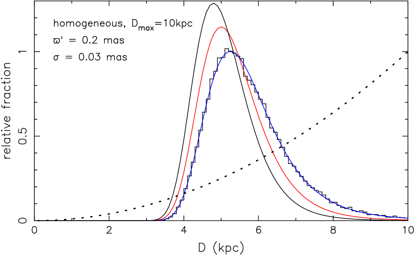
?figurename? 1: The probability distribution of actual distances for a measured parallax for objects distributed homogeneously in a finite sphere; for values of $\varpi^{\prime}$, $\sigma$ and $D_{\mathrm{max}}$ as indicated. The blue line represents Eq.18. The histogram gives the results of a Monte Carlo simulation which retains objects with $0.198<\varpi^{\prime}<0.202$. The black and red line represent modified versions of Eq.18 according to Faucher-Giguère & Kaspi (2006) and Verbiest et al. (2012), respectively. The intrinsic distribution given by Eqs.4,5 is shown as a dashed line. All curves are normalized to the same area under the curve

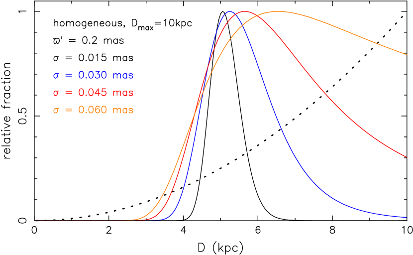
?figurename? 2: The probability distribution of actual distances for a measured parallax $\varpi^{\prime}=0.2$ mas for various measurement errors $\sigma$, for objects distributed homogeneously in a sphere with radius $D_{\mathrm{max}}=10$ kpc. The intrinsic distribution given by Eqs.4,5 is shown as a dashed line. The curves are normalized to the same maximum value

Entering Eqs.2, 4, 5 into Eq.16, we obtain with Eq.12:

$$p_{D}(D|\varpi^{\prime})=\left\{\begin{array}[]{cc}C_{D}(0,D_{\mathrm{max}})D^{2}\exp\left[-\,{(1/D-\varpi^{\prime})^{2}\over 2\sigma^{2}}\right];\,D<D_{\mathrm{max}}\\ \\ 0;\quad D>D_{\mathrm{max}}\end{array}\right.$$ (18)

In Fig.1 we plot $p_{D}(D|\varpi^{\prime})$ according to Eq.18, computing $C_{D}(0,D_{\mathrm{max}})$ numerically, for a measured parallax $\varpi^{\prime}=0.2$ mas, maximum distance $D_{\mathrm{max}}=10$ kpc and $\sigma=0.03$ mas. Fig.2 illustrates the effect of varying measurement accuracies. As the error decreases, the most probable distance closes in to the nominal measured value $1/\varpi^{\prime}$, but the probability distribution of the actual distances remains asymmetric, i.e. non-gaussian, even for small measurement errors.

To show that our approach is in agreement with that of Lutz & Kelker (1973), we note that for a homogeneous distribution in space $f_{\varpi}(\varpi)\Delta\varpi=f_{D}(D)\Delta D\propto D^{2}\Delta D$, hence $f_{\varpi}(\varpi)\propto\varpi^{-2}d(1/\varpi)/d\varpi\propto\varpi^{-4}$. This allows us to write the joint probability of a pulsar to have measured parallax $\varpi^{\prime}$ and actual parallax $\varpi$ analogous to Eq.15 as

$$P_{\varpi}(\varpi^{\prime},\varpi)\Delta\varpi^{\prime}\Delta\varpi = g_{\varpi}(\varpi^{\prime}|\varpi)\Delta\varpi^{\prime}\,f_{\varpi}(\varpi)\Delta\varpi$$ (19)

$$\propto {\Delta\varpi\over\varpi^{4}}g(\varpi^{\prime}|\varpi)\,\Delta\varpi^{\prime}$$

thus confirming the $\varpi^{-4}$ dependence found by Lutz & Kelker.

3.2 Galactocentric distribution

Entering Eqs.2, 4, 6 into Eq.16, we obtain with Eq.12:

$$p_{D}(D|\varpi^{\prime}) = C_{D}(0,\infty)D^{2}\,R^{1.9}\exp\left[-{|z(D,b)|\over h}-{R(D,l,b)\over H}\right]$$ (20)

$$\times\exp\left[-\,{(1/D-\varpi^{\prime})^{2}\over 2\sigma^{2}}\right]$$

Fig.3 illustrates this distribution for the parameters of PSR J0218+4232.

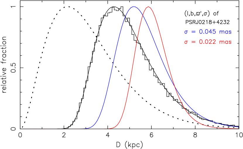
?figurename? 3: For an assumed galactocentric distribution of objects, the distribution as a function of distance to Earth is given by Eqs.4,6, illustrated for the direction towards PSR J0218+4232 with the dotted line. The black smooth line gives the probability distribution of actual distances in this direction for the measured parallax of this pulsar, according to Eq.20, in the approximation $C_{D}(0,\infty)\simeq C_{D}(0,D_{\mathrm{max}})$, $D_{\mathrm{max}}=10$ kpc. The histogram gives the results of a Monte Carlo simulation which retains objects with $0.14<\varpi^{\prime}<0.18$. The blue and red lines give the analytic distributions for hypothetically smaller measurement errors but the same value for $\varpi^{\prime}$. The curves are normalized to the same maximum value

3.3 Earlier studies

Previous authors have given different expressions for $p_{D}(D|\varpi^{\prime})$. To understand the difference between our Eqs.18,20 and these expressions, we consider the measurement process expressed in Eq.15. Consider a class of objects distributed in space according to $f_{D}(D)$ (Eq.4). The measurement process starts with the selection of one object whose parallax we wish to measure. This corresponds to taking a draw from the $f_{D}(D)$ distribution. Then the parallax is measured. The measurement refers to the unique distance $D$ of the selected object, i.e. the selection from $g_{D}(\varpi^{\prime}|D)$ is taken for a unique and fixed value of $D$.

We illustrate this separation between object selection and parallax measurement with a Monte Carlo experiment, as follows. We choose a distance $D$ randomly from a $D^{2}$ distribution (corresponding to a homogeneous distribution in a sphere) with maximum distance 10 kpc; for the distance $D$ a measured parallax $\varpi^{\prime}$ is drawn randomly from a Gaussian distribution according to Eq.2 with $\sigma=0.03$ mas. We retain the distance if $0.198<\varpi^{\prime}\mathrm{(mas)}<0.202$, and repeat the procedure until $50\,000$ distances are retained. The binned distribution of the distances $D$ of the retained objects is normalized and also plotted in Fig.1. It agrees with Eq.18. In analogous fashion we perform a Monte-Carlo experiment for the galactocentric distribution, for parameters of the millisecond pulsar PSR J0218+4232, and show in Fig.3 that the result agrees with the analytic solution given by Eq.20.

Faucher-Giguère & Kaspi (2006) write the probability of distance $D$ for a measured parallax $\varpi^{\prime}$ as (see their Eq. 2):

$$p(D|\varpi^{\prime})={C\over D^{2}}\,{1\over\sqrt{2\pi}\sigma}\exp\left[-\,{(1/D-\varpi^{\prime})^{2}\over 2\sigma^{2}}\right]$$ (21)

where $C$ (in our notation) is the normalization constant. In doing so they make two, related, errors. First, they interpret the right hand side of Eq.1 as giving the probability that the real parallax is $\varpi$ when the measured value is $\varpi^{\prime}$, when in fact it gives the probability of measuring $\varpi^{\prime}$ when the real parallax is $\varpi$. As we explain in Sect.1, this is incorrect, and arises from confusing the frequentist and Bayesian methods. Second, by interpreting the right hand side of Eq.1 as a probability density for $\varpi$, they add the factor $|d\varpi/dD|=1/D^{2}$ in converting this to a probability density for $D$; and ignore the spatial density $f(D)$. As may be seen from Eqs.2, 14 and 15 this corresponds effectively to assuming $f(D)\propto 1/D^{2}$. The effect of this double error for a homogeneous spatial distribution is to replace the $D^{2}$ factor in our Eqs.18 with $D^{-2}$, and is illustrated in Fig.1.

Verbiest et al. (2012) and Verbiest & Lorimer (2014) make the same errors as Faucher-Giguère and Kaspi (2006), but correctly include $f(D)$ into the probability density $P_{D}(D|\varpi^{\prime})$. The net effect of this is to remove the $D^{2}$ factor in our Eqs.18 and 20, which correponds to the assumption of a uniform distance distribution $f_{D}=1$. The result is illustrated in Fig.1 for a homogeneous spatial distribution.

Francis (2014) argues that the distance probability distribution is a Gaussian centered on the real value, because it collapses to the real value when the measurement error goes to zero. The effect of the spatial distribution prior $D^{2}\mathcal{F}$ does diminish when the parallax measurement error becomes smaller, because a smaller range of $D$ leads to a smaller variation of the prior $D^{2}\mathcal{F}$. Thus, for smaller errors the distance probability distribution narrows towards the correct distance. However, even for small errors, the distance probability function remains asymmetric (Figs.2 and 3). Indeed, Eq.3.2 from Francis (2014) is wrong, and confuses the frequentist and Bayesian approach, as does his conclusion that the distance distribution is irrelevant for the derivation of the probability density for the distance.

4 Distance and luminosity from parallax and flux, with assumed distance and luminosity distributions

We now consider sources for which parallax and flux have been measured, and the spatial distribution and luminosity function are known or assumed. The joint probability for $D,\varpi^{\prime},L,S^{\prime}$ may be written with Eqs.2,4,3 as

$$P(D,\varpi^{\prime},L,S^{\prime})\propto g_{D}(\varpi^{\prime}|D)f_{D}(D)g_{S}(S^{\prime}|S[L,D])f_{L}(L)=$$

$$\phantom{.}\hskip 28.45274pt{1\over\sqrt{2\pi}\,\sigma}\exp\left[-\,{(1/D-\varpi^{\prime})^{2}\over 2\sigma^{2}}\right]D^{2}\mathcal{F}(D)\times$$

$$\phantom{.}\hskip 56.9055pt{1\over\sqrt{2\pi}\,\sigma_{S}}\exp\left[-{(L/[L_{o}D^{2}]-S^{\prime})^{2}\over 2{\sigma_{S}}^{2}}\right]\,f_{L}(L)$$ (22)

For fixed values of $\varpi^{\prime}$, $\sigma$, $S^{\prime}$ and $\sigma_{S}$, and for a chosen luminosity function $f_{L}(L)$, this joint probability can be computed for each combination of $D$ and $L$. We show contours of equal probability in the $D,L$-plane in Fig.4, as applicable to PSR J0218+4232. The maximum probabilities lie at distances well below the nominal distance $D^{\prime}=1/\varpi^{\prime}$ and at luminosities well below the nominal luminosity $L^{\prime}=L_{o}S^{\prime}/{\varpi^{\prime}}^{2}$. This is due to the luminosity functions, that peak at values well below $L^{\prime}$, and thus favour low luminosities, hence small distances, as far as the measurement uncertainties allow.

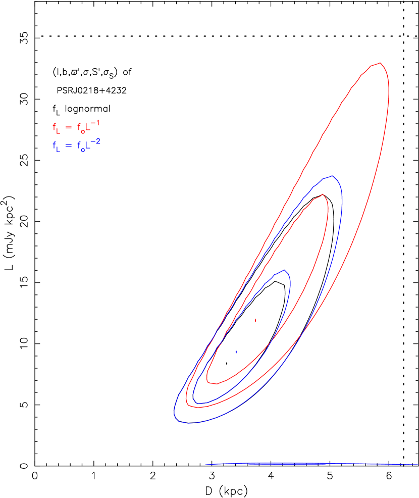
?figurename? 4: Contours of equal joint probability $P(D,\varpi^{\prime},L,S^{\prime})$, for the direction, parallax, flux, and measurement errors of PSR J0218+4232, for two power-law and for the lognormal luminosity functions. For each luminosity function we show the maximum, and contours containing 68% and 95% of the integrated probability. The contours for the power-law luminosity function with index $-2$ have two branches, one at very low luminosities, and one at higher luminosities; part of the latter is indistinguishable from the contours for the the lognormal luminosity function. The vertical and horizontal dashed lines show the nominal values for distance $D=1/\varpi^{\prime}$ and luminosity $L^{\prime}=S^{\prime}/{\varpi^{\prime}}^{2}$, respectively

In Fig. 4 we did not apply cutoffs to the power-law luminosity functions at low or high luminosity. As may be seen from Eq.22 such cutoffs do not change the form of the contours of $P(D,\varpi^{\prime},L,S^{\prime})$, but only the normalization, in the range $L_{\mathrm{min}}<L<L_{\mathrm{max}}$. Outside this range $P(D,\varpi^{\prime},L,S^{\prime})=0$.

4.1 Distances

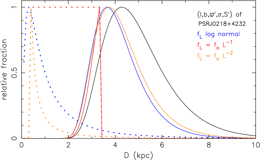
?figurename? 5: The distance probability function determined from parallax and accurate flux, with known spatial and luminosity distributions. The black line gives the values based on parallax only (reproducing the black line in Fig.3). For a lognormal luminosity function, the dashed blue line shows the extra term $D^{2}f_{L}(L_{o}D^{2}S^{\prime})$ and the blue solid line the overall distribution according to Eq.24, for values appropriate for PSR J0218+4232. The dashed and solid red and brown lines idem for power-law luminosity functions both with $L_{\mathrm{min}}=0.1$ mjy kpc², and $L_{\mathrm{max}}=10$ mJy kpc² for $\alpha=-1$, and $L_{\mathrm{max}}=100$ mJy kpc² for $\alpha=-2$, respectively. All curves are normalized to their maximum value.

Suppose that we are interested in the probability distribution for distances only. We note that, for a finite measurement error, a range of luminosities contributes to the probability of measuring $S^{\prime}$. By integrating over the luminosity, we find the joint probability of $D,\varpi^{\prime},S^{\prime}$

$$P(D,\varpi^{\prime},S^{\prime})\propto g_{D}(\varpi^{\prime}|D)f_{D}(D)\int g_{S}(S^{\prime}|S[L,D])f_{L}(L)dL=$$

$$\phantom{M}g_{D}(\varpi^{\prime}|D)f_{D}(D)\int g_{S}(S^{\prime}|S[L,D])f_{L}(L_{o}D^{2}S))\,L_{o}D^{2}dS$$ (23)

where we use the fact that $g_{D}(D)$ and $f_{D}(D)$ do not depend on $L$.

In many applications, the flux is measured much more accurately than the parallax, in the sense that $\sigma_{S}/S\ll 1$. In that case, for a measurement error distribution $g_{S}$ according to Eq.3, only values of $S$ close to $S^{\prime}$ contribute to the integral over $S$ in Eq.23, and $f_{L}$ is close to constant in that small interval. Thus the factor $f_{L}(L_{o}D^{2}S)L_{o}D^{2}=f_{L}(L_{o}D^{2}S^{\prime})L_{o}D^{2}$ may be written outside of the integral, and the remaining integral $\int g_{S}(S^{\prime}|S)dS=1$. With Bayes’ theorem we then obtain (cf. Eqs.12, 13):

$$p_{D}(D|\varpi^{\prime},S^{\prime}) = C_{D}(0,D_{\mathrm{max}})D^{2}\mathcal{F}(D)\times$$ (24)

$$\exp\left[-{(1/D-\varpi^{\prime})^{2}\over 2\sigma^{2}}\right]L_{o}D^{2}f_{L}(L_{o}D^{2}S^{\prime})$$

Apart from normalization, the only difference with Eqs.18 and 20 is the extra term $D^{2}f_{L}(L_{o}D^{2}S^{\prime})$. For $f_{L}\propto L^{-1}$, the extra term $D^{2}f_{L}$ is constant, and thus $p_{D}(D|\varpi^{\prime},S^{\prime})$ (Eq.24) is identical to $p_{D}(D|\varpi^{\prime})$ , except for a normalization constant, provided $L_{\mathrm{min}}<L<L_{\mathrm{max}}$.

In Fig.5 we apply eq. 24 to PSR J0218+4232, for three luminosity functions, where we set the uncertainty of the measured flux to zero, for illustrative purpose .

For the power-law luminosity function Eq.8 with $\alpha=-1$ we fix minimum and maximum luminosities at 0.1 mJy kpc² and 10 mJy kpc², respectively. The accurate flux then leads to minimum and maximum distances at: $D_{\mathrm{min}}=\sqrt{L_{\mathrm{min}}/L_{o}S^{\prime}}=0.33$ kpc and $D_{\mathrm{max}}=\sqrt{L_{\mathrm{max}}/L_{o}S^{\prime}}=3.3$ kpc. For this luminosity function $p_{D}(D|\varpi^{\prime},S^{\prime})\propto p_{D}(D|\varpi^{\prime})$ in the range $L_{\mathrm{min}}<L<L_{\mathrm{max}}$.

For a steeper power law with $\alpha=-2$, the extra term $D^{2}f_{L}\propto D^{-2}$ enhances the probability of lower distances and lowers the probability of large distances. We show this for $L_{\mathrm{max}}=100$ mJy kpc².

In Fig.5 we also show Eq.24 for the lognormal distribution, applied to PSR J0218+4232, which apart from the normalization is rather similar to the result for a power-law luminosity distribution with $\alpha=-2$.

For all three luminosity functions, the lower range of allowed distances is determined mainly by the parallax and its error.

4.2 Distances: earlier derivations

Verbiest et al.  (2012) use the lognormal luminosity function Eq.10. Entering this in Eq.24 we obtain

$$p_{D}(D|\varpi^{\prime},S^{\prime}) = C_{D}(0,D_{\mathrm{max}})D^{2}\mathcal{F}(D)\exp\left[-\,{(1/D-\varpi^{\prime})^{2}\over 2\sigma^{2}}\right]\times$$ (25)

$$\exp\left[-\,{(\log\left[L_{o}D^{2}S^{\prime}\right]-\mu_{x})^{2}\over 2{\sigma_{x}}^{2}}\right]{1\over S^{\prime}}$$

Comparing this with Eq.26 of Verbiest et al. (2012), we see that the $1/S^{\prime}$ term in Eq.25 is there replaced with $1/D$. This variant arises because their Eq. 25 has $d\lambda/dD$ instead of the correct $d\lambda/dS^{\prime}$, analogous to the error leading to Eq.21. As a result, the probability of actual distance for measured parallax and flux given by Verbiest et al. (2012, their Eq. 27), has a weighting factor $1/D^{3}$, absent in the correct version of our Eq.25 (and omits the weighting factor $1/S^{\prime}$, which however drops out in the normalization).

4.3 Luminosities

In the case where we are interested in luminosities only, we write the joint probability of $L$, $\varpi^{\prime}$ and $S^{\prime}$, averaged over distances $D$, by integrating Eq.22 over $D$. Substituting $D=\varpi^{-1}$, and $D_{\mathrm{max}}=1/\varpi_{\mathrm{min}}$ this leads to

$$P(L,\varpi^{\prime},S^{\prime}) \propto f_{L}(L)\int_{\varpi_{\mathrm{min}}}^{\infty}{\varpi^{-2}\mathcal{F}({1\over\varpi})\over\sqrt{2\pi}\,\sigma}\exp\left[-{(\varpi-\varpi^{\prime})^{2}\over 2\sigma^{2}}\right]\times$$ (26)

$${1\over\sqrt{2\pi}\sigma_{S}}\exp\left[-{(L\varpi^{2}/L_{o}-S^{\prime})^{2}\over 2{\sigma_{S}}^{2}}\right]\,\varpi^{-2}d\varpi$$

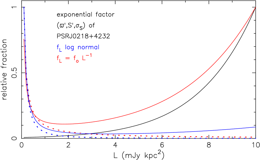
?figurename? 6: The luminosity probability function determined from accurate parallax and uncertain flux (values for PSR J0218+4232), with two assumed luminosity distributions. The black line gives the exponential factor in Eq.28. The dashed red line shows a power-law luminosity function, and the solid red line the product of this with the exponential. The blue lines idem for a lognormal luminosity function. Because of the accurate distance, this luminosity probability function is valid for any spatial distribution

4.3.1 Luminosities with accurate distance

We first consider the case where the distance is well known, in the sense that $\sigma/\varpi\ll 1$. Only terms with $\varpi\simeq\varpi^{\prime}$ contribute to the integral over $\varpi$ in Eq.26, which may be rewritten as

$$P(L,\varpi^{\prime},S^{\prime}) \propto f_{L}(L){\varpi^{\prime}}^{-4}\mathcal{F}\left({1\over\varpi^{\prime}}\right)\exp\left[-{(L{\varpi^{\prime}}^{2}/L_{o}-S^{\prime})^{2}\over 2{\sigma_{S}}^{2}}\right]\times$$ (27)

$$\int_{\varpi_{\mathrm{min}}}^{\infty}{1\over\sqrt{2\pi}\,\sigma}\exp\left[-{(\varpi-\varpi^{\prime})^{2}\over 2\sigma^{2}}\right]\times d\varpi$$

The integral is a constant for a given $\varpi_{\mathrm{min}}\equiv 1/D_{\mathrm{max}}$, and approaches unity when $\sigma/\varpi^{\prime}$ approached zero, provided $\varpi^{\prime}>\varpi_{\mathrm{min}}$, i.e. provided that the nominal distance $D^{\prime}\equiv 1/\varpi^{\prime}$ satisfies $D^{\prime}<D_{\mathrm{max}}$. We then have

$$p_{L}(L|\varpi^{\prime},S^{\prime}) = C_{L}(L_{\mathrm{min}},L_{\mathrm{max}}){\varpi^{\prime}}^{-4}\mathcal{F}({1\over\varpi^{\prime}})f_{L}(L)$$

$$\times\exp\left[-{[L-L^{\prime}(\varpi^{\prime},S^{\prime})]^{2}\over 2{\sigma_{S}(\varpi^{\prime})}^{2}}\right]$$

$$\mathrm{where} L^{\prime}(\varpi^{\prime},S^{\prime})={L_{o}S^{\prime}\over{\varpi^{\prime}}^{2}};\quad\sigma_{S}^{\prime}(\varpi^{\prime})={L_{o}\sigma_{s}\over{\varpi^{\prime}}^{2}}$$ (28)

Because the integral over $L$ implicit in $C_{L}(L_{\mathrm{min}},L_{\mathrm{max}})$ does not depend on $D$, the factor $D^{4}\mathcal{F}={\varpi^{\prime}}^{-4}\mathcal{F}({1/\varpi^{\prime}})$ may be dropped from this equation. Specifically, this implies that $p_{L}(L|\varpi^{\prime},S^{\prime})$ does not depend on the spatial distribution. Eq.28 can be interpreted directly, as follows. For an accurate distance $D=1/\varpi^{\prime}$, the number of sources scales with $D^{2}\mathcal{F}$. An extra factor $D^{2}$ is due to the conversion of a flux interval $\Delta S$ to a luminosity interval $\Delta L$. The probability of luminosity $L$ is given by the probability of the corresponding flux $S=L/(L_{o}D^{2})$, weighted with the luminosity function $f_{L}$. The weighting factor $f_{L}$ in general may cause the most probable luminosity to differ from the nominal luminosity $L^{\prime}=L_{o}D^{2}S^{\prime}$ – analogous to the way in which the weighting factor $f_{D}$ causes the most probable distance to differ from the nominal distance $D^{\prime}=1/\varpi^{\prime}$ in Eqs.18 and Eq.20.

The effect of the competition between the luminosity function $f_{L}$ and the exponential term in Eq.28 can be quite dramatic, as illustrated in Fig.6. As an example we consider PSR J0218+4232, assuming for illustrative purpose that its parallax is exact. With $L_{o}=1$, its nominal luminosity is $L^{\prime}=L_{o}S^{\prime}/{\varpi^{\prime}}^{2}\simeq 35$ mJy kpc², and $\sigma_{S}^{\prime}\simeq 8$ mJy kpc². In the luminosity range considered, $0.1<L(\mathrm{mJykpc}^{2})<10$, the exponential factor in Eq.28 increases by a factor 130 between the low and the high luminosity limit. The relatively flat luminosity function $f_{L}\propto L^{-1}$ decreases by a factor 100 in the same range. As a result, the overal luminosity probability peaks both at 0.1 mJy kpc², and – less steeply – at 10 mJy kpc².

The peak at the high luminosity limit is lowered for a luminosity function that drops faster towards high luminosities, as illustrated in Fig.6 for the lognormal distribution Eq.10. For a power law $f_{L}\propto L^{-2}$ the peak at 10 mJy kpc² disappears. On the other hand, if the flux measurement error is halved from its actual value to $\sigma_{S}=0.1$ mJy, both power-law distributions and the lognormal distribution all combine with the exponential function to give a peak only at 10 mJy kpc² in the relative probability.

4.3.2 Luminosities with accurate flux

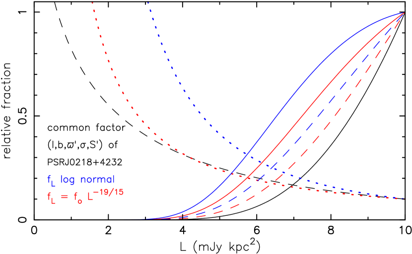
?figurename? 7: The luminosity probability function determined from uncertain parallax and accurate flux (values for PSR J0218+4232). The black solid line shows the exponential factor in Eq.30, multiplied with $L^{1.5}$, the black dashed line shows $\mathcal{F}$. In blue, the dotted curve shows the lognormal luminosity distribution, the dashed and solid curves the corresponding luminosity probability functions for homogeneous and galactocentric spatial distributions, respectively. In red, idem for the power-law luminosity function. All curves are normalized to a value 1 at 10 kpc, except those for the luminosity functions and for $\mathcal{F}$, normalized to a value of 0.1 at 10 kpc

To compute the integral in Eq.26 in the limit $\sigma_{s}/S^{\prime}\ll 1$, we first make the substitution $\varpi^{2}=uL_{o}/L$, hence $2\varpi d\varpi=du\,L_{o}/L$. Only terms with $u\simeq S^{\prime}$ contribute to the integral, hence

$$P(L,\varpi^{\prime},S^{\prime}) \propto f_{L}(L)x^{-5}\mathcal{F}\left({1\over x}\right)\exp\left[-{(x-\varpi^{\prime})^{2}\over 2\sigma^{2}}\right]\times$$

$$\int_{u_{\mathrm{min}}}^{\infty}\exp\left[-{(u-S^{\prime})^{2}\over 2{\sigma_{S}}^{2}}\right]du\,{L_{o}\over L}$$

$$\mathrm{where} x=\sqrt{L_{o}S^{\prime}\over L};\quad\mathrm{and}\quad u_{\mathrm{min}}={\varpi_{\mathrm{min}}}^{2}{L\over L_{o}}$$ (29)

The integral depends on $L$, via $u_{\mathrm{min}}$. However, provided that $S^{\prime}>u_{\mathrm{min}}$, i.e. $L<L_{o}{D_{\mathrm{max}}}^{2}S^{\prime}$, the integral approaches unity when $\sigma_{s}/S^{\prime}$ approaches zero. For $L>L_{o}{D_{\mathrm{max}}}^{2}S^{\prime}$ the integral approaches zero in the same limit. Thus

$$p_{L}(L|\varpi^{\prime},S^{\prime})=\left\{\begin{array}[]{l}C_{L}(L_{\mathrm{min}},L_{\mathrm{max}})f_{L}(L)\left({L\over L_{o}S^{\prime}}\right)^{5/2}{L_{o}\over L}\mathcal{F}\left(\sqrt{L\over L_{o}S^{\prime}}\,\right)\times\\ \phantom{m}\exp\left[-{(\sqrt{L_{o}S^{\prime}/L}-\varpi^{\prime})^{2}\over 2\sigma^{2}}\right]\,\mathrm{for}\,L<L_{o}{D_{\mathrm{max}}}^{2}S^{\prime}\\ \\ 0\quad\mathrm{for}\quad L>L_{o}{D_{\mathrm{max}}}^{2}S^{\prime}\end{array}\right.$$ (30)

Because the integral over $L$ implicit in $C_{L}(L_{\mathrm{min}},L_{\mathrm{max}})$ does not depend on $L_{o}$ or $S^{\prime}$, the factor $L_{o}(L_{o}S^{\prime})^{-5/2}$ may be omitted from Eq.30.

For the flux and parallax of PSR J0218+4232, the exponential factor in Eq.30 increases with $L$ up to 10 mJy kpc² (and beyond), and this increase is amplified by the factor $L^{1.5}$. In contrast, the luminosity functions increase towards the minimum luminosity of 0.1 mJy kpc². The combined effect of these two factors is shown in Fig.7. The luminosity probability for the galactocentric distribution observed in the direction of PSR J0218+4232, has a stronger contribution at luminosities below 10 mJy kpc² than the homogeneous distribution. This is due to the rise of $\mathcal{F}$ towards lower distances, hence lower luminosities.

4.3.3 Can we do without the luminosity function?

Since the luminosity is given by $L=L_{o}D^{2}S^{\prime}$, one may wonder whether, in the case of accurate flux, the probability of luminosity follows the probability of distance squared:

$$p_{L}(L|\varpi^{\prime},S^{\prime})\mathrel{\hbox{\hbox to0.0pt{\lower 0.21529pt\hbox{$=$}\hss} \kern-2.29996pt\raise 4.73611pt\hbox{\footnotesize?}}}K\,p_{D^{2}}(D^{2}|\varpi^{\prime})$$ (31)

where $K$ is a proportionality constant. The answer is no. This is most easily seen if we consider a standard candle, where the luminosity function is unity for $L=L_{S}$ and zero for all other luminosities $L\neq L_{S}$. An accurate flux then implies that only one distance is possible, viz. the one for which $L_{o}S^{\prime}D^{2}=L_{S}$, whereas the right hand side of Eq.31 gives a non-zero value for a range of distances.

More generally, at fixed flux $S^{\prime}$ a different part of the luminosity function $f_{L}$ is sampled at different distances, and thus the luminosity function is indispensable in the determination of probabilities.

The invalidity of Eq.31 implies that the probability density function of the luminosity can be given only when the luminosity function is known or assumed, or alternatively when also the parallax is very accurate.

5 The distance and gamma-ray luminosity of PSR J0218+4232

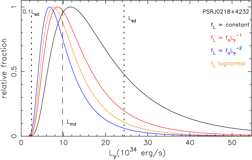
?figurename? 8: The gamma-ray luminosity probability function determined from the parallax with error and accurate gamma-ray flux of PSR J0218+4232, for three different assumed power-law and one lognormal gamma-ray luminosity functions. The realistic distance prior (Eqs. 4, 6) is assumed. $L_{\mathrm{sd}}$ (Eq. 32), and $0.1L_{\mathrm{sd}}$ are indicated with vertical dotted lines, $L_{\mathrm{md}}$ (Eq. 34) is indicated with a vertical dashed line.

?figurename? 9: The gamma-ray luminosity probability function determined from the parallax with error and accurate gamma-ray flux of PSR J0218+4232, for three different distance priors and two different luminosity priors. $L_{\mathrm{sd}}$ (Eq. 32), and $0.1L_{\mathrm{sd}}$ are indicated with vertical dotted lines, $L_{\mathrm{md}}$ (Eq. 34) is indicated with a vertical dashed line.

An upper limit to the rotation-powered gamma-ray luminosity $L_{\gamma}$ is given by the spindown luminosity $L_{\mathrm{sd}}$

$$L_{\mathrm{sd}}\equiv{4\pi^{2}I\dot{P}\over P^{3}}\simeq 2.44\times 10^{35}\mathrm{erg/s}$$ (32)

where the numerical value is for PSR J0218+4232 (see Table 1), with an assumed moment of inertia $I=10^{45}\mathrm{g\,cm}^{2}$ for the neutron star. It should be noted that the moment of inertia $I$ of the neutron star PSR J0218+4232 is uncertain, as its mass and radius are uncertain.

As reference values we use the nominal gamma-ray luminosity, at the nominal distance $D_{\mathrm{n}}\equiv 1/\varpi^{\prime}=6.25$ kpc:

$$L_{\mathrm{n}}\equiv 4\pi{1\over{\varpi^{\prime}}^{2}}\,S_{\gamma}=2.1\times 10^{35}\mathrm{erg/s}=0.87L_{\mathrm{sd}}$$ (33)

and the luminosity at the most probable distance according to Eq.19, $D_{\mathrm{md}}=4.28$ kpc

$$L_{\mathrm{md}}\equiv 4\pi{D_{\mathrm{md}}}^{2}\,S_{\gamma}=9.8\times 10^{34}\mathrm{erg/s}=0.40L_{\mathrm{sd}}$$ (34)

Note that the gamma-ray luminosity is defined for isotropic emission (i.e. $S_{o}=4\pi$), which the gamma pulsations show to be false.

As noted in the previous section, the probability distribution of luminosity for measured parallax with error and accurate flux, can be given only when a luminosity function is known or assumed.

The effect of using different priors is illustrated in Figures 8 and 9 and in Tables 2 and 3.

Table 2 shows that use of a realistic distance prior, $f_{D}\propto D^{2}\mathcal{F}$ with $\mathcal{F}$ given by Eq. 6, reduces the most probable distance to a value smaller than for $f_{D}$ uniform or spatially homogeneous, also when $f_{L}$ is implemented. Application of realistic luminosity priors narrows the $95\%$ distance credibility interval, in particular when an upper bound to $L_{\gamma}$ is set equal to $L_{\mathrm{sd}}$. In this case the upper limit of the credibility interval is close to the nominal distance of $6.25$ kpc.

Figure 8 shows the probability density functions of $L_{\gamma}$ for the realistic distance prior $f_{D}\propto D^{2}\mathcal{F}$ with $\mathcal{F}$ given by Eq. 6. For each luminosity prior the probability that $L_{\gamma}<L_{\mathrm{sd}}$ is very small, $<0.001$, and the most probable luminosity $L_{\mathrm{mp}}$ is well above $0.1L_{\mathrm{sd}}$ and well below $L_{\mathrm{sd}}$. For steeper luminosiy functions the probability density function is pushed to lower luminosities, as expected (see Table 3).

The influence of the distance prior is much more significant. The unrealistic distance priors, combined with the large uncertainty in the parallax, lead to unreallistically high $L_{\gamma}>L_{sd}$, especially for the uniform luminosity prior.

?tablename? 2: The most probable distance $D_{\mathrm{mp}}$ and $95\%$ credibility interval for different distance and luminosity priors for PSR J0218+4232.

Priors		$D_{\mathrm{mp}}$	$D_{l}$ – $D_{u}$ (a)	$D_{l}$ – $D_{u}$ (b)
$f_{D}$	$f_{L}$	(kpc)	(kpc)	(kpc)
const	–	6.25	3.75 – 10.0	–
$D^{2}$	–	10.0	4.62 – 10.0	–
$D^{2}\mathcal{F}$	–	4.28	2.65 – 7.82	–
$D^{2}\mathcal{F}$	lognorm	3.99	2.51 – 7.15	2.71 – 6.38
$D^{2}\mathcal{F}$	$\mathrm{const}$	5.05	3.08 – 8.95	3.39 – 6.69
$D^{2}\mathcal{F}$	$L^{-1}$	4.28	2.65 – 7.82	2.97 – 6.59
$D^{2}\mathcal{F}$	$L^{-2}$	3.74	2.39 – 6.65	2.50 – 6.15

?tablename? 3: The most probable gamma-ray luminosity $L_{\mathrm{mp}}$ and $95\%$ credibility interval for different distance and luminosity priors for PSR J0218+4232.

Priors		$L_{\mathrm{mp}}$	$L_{l}$ – $L_{u}$	$\int_{L_{\mathrm{sd}}}^{\infty}p_{L}(L)dL$
$f_{D}$	$f_{L}$	($L_{\mathrm{sd}}$)	($L_{\mathrm{sd}}$)
–	–	0.87	–	–
$D^{2}$	–	2.24	$0.70$ – $2.24$	$0.86$
$\mathrm{const}$	$\mathrm{const}$	2.24	$0.48$ – $2.24$	$0.72$
$D^{2}$	$L^{-2}$	0.56	$0.24$ – $2.14$	$0.51$
$D^{2}\mathcal{F}$	$\mathrm{const}$	0.48	$0.17$ – $1.72$	0.26
$D^{2}\mathcal{F}$	$L^{-1}$	0.36	$0.13$ – $1.32$	0.12
$D^{2}\mathcal{F}$	$L^{-2}$	0.28	$0.11$ – $0.96$	0.04
$D^{2}\mathcal{F}$	lognorm	0.31	$0.12$ – $1.11$	0.07

6 Conclusions and discussion

A homogeneous spatial distribution is useful for pedagogical purposes in explaining the importance of a prior in deriving a distance probability distribution from a measured parallax. For realistic investigations, however, a homogeneous spatial distribution is rather misleading. In particular, for a homogeneous spatial distribution, the number of sources increases with distance, and a measured parallax will more often correspond to a large distance which is measured too low, than to a small distance measured too high. In this case, a parallax more often underestimates the actual distance, especially for large measurement uncertainties (see Fig.2). In a realistic galactic distribution, as observed from Earth, a parallax tends to overestimate the distance, however, at distances where the intrinsic source distribution decreases with distance (Fig.3). This is often the case, for example in directions away from the galactic center and / or away from the galactic plane.

Both analytically and via a Monte Carlo simulation, we show that a prior for the spatial distribution must be used, also in the study of a single object, for the determination of the distance probability density. Similarly, when parallax and flux measurements with their errors are combined to derive probability density distributions for distances and luminosities, priors are necessary for both spatial and luminosity distributions. The nominal distance $D^{\prime}=1/\varpi^{\prime}$ and luminosity $L^{\prime}=L_{o}S/{\varpi^{\prime}}^{2}$ may be very different from the most probable values (see Fig.4), unless both measurement erors are small. This is the consequence of the predominance of low luminosities in the luminosity functions that we use: for each flux the higher probability of a low luminosity translates into a higher probability of a lower distance – in as far as the parallax measurement allows this. In the case of PSR J0218+4232, for example, the most probable distance as derived fom the parallax only is at 4.28 kpc (Fig.5). When parallax and radio flux are both used, the most probable distance drops to 3.74  kpc and 3.42 kpc for power-law luminosity functions with index $\alpha=-1$ and $\alpha=-2$, respectively; and to 3.25 kpc for the lognormal luminosity distribution (Fig.4). Clearly, the quality of the estimates of distance and luminosity is enhanced by the use of realistic prior distributions with respect to the nominal estimates based on measurement only. On the other hand, it is important to keep in mind that wrong priors may deteriorate the estimate.

In particular the use of the spatial homogeneous prior is harmful in the case of an uncertain parallax: it shifts the value for most probable distance or luminosity to the upper boundary on the prior (see second line in Tables 2 and 3). In contrast, the realistic distance prior gives an estimate for the gamma-ray luminosity inside the physically motivated region ($L_{\mathrm{mp}}<L_{\mathrm{sd}}$) even when no additional restrictions on the luminosity function are imposed. An application of the lognormal luminosity prior gives an estimate for distance and gamma-ray luminosity which is in between two values obtained if we apply power law with $\alpha=-1$ and $\alpha=-2$.

It may be noted, in particular for the power-law luminosity function, that the luminosity function may have a different form at different luminosities (for an example, see Eq.17 of Faucher-Giguère & Kaspi 2006.) This is easily implemented in the formalism described in the previous Sections. More complicated is the – probably realistic – case where the luminosity function depends on the position in the Galaxy. For millisecond pulsars this is unlikely. Ordinary pulsars at large $z$, however, are on average older than pulsars close to the galactic plane, and may well have lower luminosities, if the pulsar luminosity depends on its period and / or period derivative. For the study of such pulsars an evolutionary model is indispensable in the determination of their distances and luminosities.

In the study of a single object, the priors of spatial and luminosity distributions must be known. In the study of a larger number of objects, however, these distributions can and indeed should be derived from prior observations. In general one may still wish to describe these distributions with a number of parameters, e.g. $H$ and $h$ in Eq.6, $\alpha$ in Eq.8, or $\mu_{x}$ and $\sigma_{x}$ in Eq.10. For a sufficiently large number of pulsars, the evolutionary model can also be tested. At the moment, such studies are hampered by the lack of reliable large ($>1$ kpc) distances.