Monte Carlo model for electron degradation in Xenon gas

Abstract

We have developed a Monte Carlo model for studying the local degradation of electrons in the energy range 9-10000 eV in xenon gas. Analytically fitted form of electron impact cross sections for elastic and various inelastic processes are fed as input data to the model. Two dimensional numerical yield spectrum, which gives information on the number of energy loss events occurring in a particular energy interval, is obtained as output of the model. Numerical yield spectrum is fitted analytically, thus obtaining analytical yield spectrum. The analytical yield spectrum can be used to calculate electron fluxes, which can be further employed for the calculation of volume production rates. Using yield spectrum, mean energy per ion pair and efficiencies of inelastic processes are calculated. The value for mean energy per ion pair for Xe is 22 eV at 10 keV. Ionization dominates for incident energies greater than 50 eV and is found to have an efficiency of $\sim$65% at 10 keV. The efficiency for the excitation process is $\sim$30% at 10 keV.

1 Introduction

When electrons interact with atoms or molecules, energy of the incident electron is lost through inelastic collisions with the target. The target atom can undergo ionization or excitation. Secondary electrons released during ionization process will trigger further collisions. These electrons lose energy via further collisions in the gas. This kind of electron energy degradation process is of great importance in understanding phenomena, like electron beam propagation in the atmosphere, population inversion process in a large group of gas lasers, optical emissions occurring in the upper atmosphere, like aurora and airglow which happen due to the precipitation of high energy electrons, etc [1, 2, 3, 4].

Xenon is a widely studied atom due to its inert nature and simple ground state atomic structure. The inert nature of xenon makes it possible to study the pristine environment of the early solar system whose traces have been removed by other reactive elements. Noble gases are valuable probes of extraterrestrial environments. Their abundances as well as isotopic compositions are indicators of various processes such as stellar events prior to solar system formation and radioactive decay. Hence their study is vital to understand the sequence of events that led to the formation and subsequent evolution of the solar system. There are various missions that studied xenon in planetary atmospheres. For example, Galileo mass spectrometer reported a relative abundance of 2.6$\pm$0.5 times solar ratios in Jovian atmosphere [5]. Pioneer Venus Sounder Probe Neutral Mass Spectrometer measured an upper limit for xenon in Venusian atmosphere as 120 ppb [6]. In Earth’s atmosphere xenon is a trace gas, having a concentration of 87 ppb [7].

Electron collision with Xe has a wide range of application. In x-ray and gamma ray detectors, Xe gas counters have been commonly used. In both these detectors, interaction of radiation with Xe atoms results in the production of electrons. Among the various methods of amplifying the obtained skimp signal, a commonly used approach is electron acceleration in which the accelerated electrons excite the xenon atoms through inelastic collisions leading to the production of secondary scintillation, i.e. the emission of detectable light in the vacuum ultraviolet region[8]. The same technique is used in flash lamps which produce high intensity white light for a short duration. The excited atoms, created by electron-atom collisions, can de-excite by emitting in different wavelengths whose combined effect will give the appearance of white light emission. Electron bombardment technique with xenon is also used in ion thrusters which is an evolving technology in the field of rocket propulsion. Here, electrically accelerated Xe ions, created using electron impact, are emitted at high speed as exhaust and this will push the spacecraft forward. Efficiency of this kind of ion thrusters are found to be higher than that of conventional chemical propulsion methods and has been used in NASA’s missions Deep Space-1 [9] and DAWN [10]. The utmost use of xenon gas for such purposes will be possible only through a thorough understanding of properties associated with microscopic collision processes.

Monte Carlo simulation is a commonly used method for studying particle energy degradation process [11, 12, 13, 14, 15, 16]. The electron collision process in xenon was studied earlier by Date et al. [17] using Monte Carlo method. Rachinhas et al. [18] studied the absorption of electrons with energies $\leq$ 200 keV in xenon using Monte Carlo simulation technique. They calculated mean energy per ion pair (w-value) and Fano factor in the energy range 20-200 keV and studied the influence of electric field on the results. Absorption of x-ray photons and the drift of resulting electrons under the influence of an applied electric field in xenon was studied by Dias et al. [19], by using Monte Carlo technique. A 3D Monte Carlo method was used by Santos et al. [20] to study the drift of electrons in xenon and to calculate various physical properties such as electroluminescence, drift velocities etc.

We have developed a Monte Carlo model for the local degradation of electrons with energy in the range 9-10000 eV in neutral xenon gas to understand how the energy of the incident electron will be distributed among various loss channels like ionization and excitation while it is making collisions with neutral xenon atoms. Using our Monte Carlo model, we have calculated numerical yield spectra which is a basic distribution function that contain information regarding the degradation process and can be used to calculate the yield of any excited or ionized states. The numerical yield spectra is then fitted analytically, thus obtaining analytical yield spectra. For practical purposes, the use of analytical yield spectrum simplify the application by substantially reducing the computational time. We have also obtained secondary electron energy distribution, the efficiency of excitation and ionization processes, as well as the mean energy expended for ion pair production.

2 Monte Carlo model

In the Monte Carlo simulation, the energy loss process of the electron is treated in a discrete manner. In carrying out the degradation by means of discrete steps, the electron is followed as it undergoes successive collisions. To accomplish the energy degradation in a convenient way, the energy range from the incident energy to cut off energy is divided into a number of equally spaced bins. Whenever an electron makes an inelastic collision, the collision event is recorded in the corresponding energy bin. This process is continued and the particle, its secondaries, tertiaries, etc. are followed until their energy falls below an assigned cut off value.

The energy bin size is taken as 1 eV throughout the energy range. To make an inelastic collision with a xenon atom, an electron should have a minimum energy of 8.315 eV as it is the lowest threshold of all the inelastic processes. We have set the cut off as 9 eV since we have 1 eV energy bins in the model.

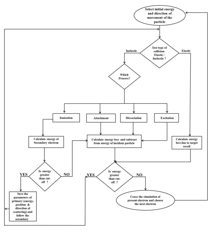
Figure 1: Flowchart showing Monte Carlo simulation for electron degradation. Figure shows flow only up to secondary electrons; subsequent electrons (tertiary, quaternary etc.) are also followed in the similar manner in the simulation.

Figure 1 shows the flow diagram for our Monte Carlo simulation for electron degradation. The simulation starts by fixing the energy of the incident electron. The direction of movement of electron ($\theta$, $\phi$) is assumed to be isotropic. The distance that the electron has to travel before the collision is calculated as

$$S=-\log(1-R)/N\sigma_{T},$$ (1)

where R is a random number, N is the number density of the gas (equal to 10¹⁰ cm^-3) and $\sigma_{T}$ is the total scattering cross section (elastic + inelastic). Next we decide on the type of collision. The probabilities of the elastic and inelastic events, P_el($\sigma_{el}$/ $\sigma_{T}$) and P_in ($\sigma_{in}$/ $\sigma_{T}$), where $\sigma_{el}$ and $\sigma_{in}$ are elastic and inelastic cross sections, are calculated and compared with new random number R₄. Elastic collision occurs if P_el $\geq$ R₄. The energy loss in elastic collisions $\Delta$E due to target recoil is calculated as

$$\bigtriangleup E=\frac{m^{2}v^{2}}{m+M}-\frac{m^{2}vV_{1}\cos\delta}{m+M},$$ (2)

where

$$V_{1}=v\left[\frac{m\cos\delta}{m+M}+\frac{[M^{2}+m^{2}(\cos\delta-1)]^{1/2}}{m+M}\right].$$

Here $\delta$ is the scattering angle in the laboratory frame, $v$ and $m$ are, respectively, the velocity and mass of the incident electron, and $M$ is the mass of the target particle. The scattering angle $\delta$ is determined by using differential elastic cross sections which are fed numerically into the model. The energy lost in the collision is then subtracted from the incident electron energy. After the collision, the deflection angle relative to the direction ($\theta$,$\phi$) is obtained by

$$\cos\theta^{{}^{\prime\prime}}=\cos\theta\cos\theta^{{}^{\prime}}-\sin\theta\sin\theta^{{}^{\prime}}\cos\phi^{{}^{\prime}},$$

$$\cos\phi^{{}^{\prime\prime}}=(\cos\theta\cos\phi\sin\theta^{{}^{\prime}}\sin\phi^{{}^{\prime}}-\sin\phi\sin\theta^{{}^{\prime}}\sin\phi^{{}^{\prime}}+\sin\theta\cos\phi\cos\theta^{{}^{\prime}})/\sin\theta^{{}^{\prime\prime}},$$ (3)

$$\sin\phi^{{}^{\prime\prime}}=(\cos\theta\cos\phi\sin\theta^{{}^{\prime}}\cos\phi^{{}^{\prime}}-\cos\phi\sin\theta^{{}^{\prime}}\sin\phi^{{}^{\prime}}+\sin\theta\sin\phi\cos\theta^{{}^{\prime}})/\sin\theta^{{}^{\prime\prime}}.$$

Here $\theta^{{}^{\prime}}$, $\phi^{{}^{\prime}}$ are the scattering angles.

If an inelastic collision occurs, the collision event is recorded in the appropriate energy bin corresponding to the energy of the particle. It is further decided whether it is an excitation or ionization event. In case of ionization event, the energy of secondary electron has to be calculated as it can also initiate further inelastic collisions, provided it has sufficient energy. The secondary electron energy is calculated as [21]

$$T=\frac{\Gamma_{S}\ E_{v}}{E_{v}+\Gamma_{B}}[\tan(RK_{1}+(R-1)K_{2})]+T_{S}-\left[\frac{T_{A}}{E_{v}+T_{B}}\right],$$ (4)

where

$$K_{1}=\tan^{-1}\left\{\left[\frac{(E_{v}-I)}{2}-T_{S}+\frac{T_{A}}{(E_{v}+T_{B})}\right]\bigg{/}\frac{\Gamma_{S}\ E_{v}}{(E_{v}+\Gamma_{B})}\right\},$$

$$K_{2}=\tan^{-1}\left\{\left[T_{S}-\frac{T_{A}}{(E_{v}+T_{B})}\right]\bigg{/}\frac{\Gamma_{S}\ E_{v}}{(E_{v}+\Gamma_{B})}\right\}.$$

Here $E_{v}$ is the incident electron energy; $\Gamma_{S}$, $\Gamma_{A}$, $T_{A}$, $T_{B}$, and $T_{S}$ are the fitting parameters, and $I$ is the ionization threshold. We have used the fitting parameters of Green and Sawada [21]. If this energy is greater than that of the cut off energy (9 eV) then the secondary electron has to be followed. In order to follow the secondary electron, the parameters of the primary electron, i.e. the energy remaining in the primary, its position and direction of movement are first saved in suitable variables. Secondary electron is then followed in the same method as the primary electron. Once the energy of the secondary is completely degraded, the saved parameters of the primary electron are retrieved and its degradation is continued. Similarly, tertiary, quaternary, etc., electrons are followed in the simulation.

For all inelastic collisions, the collision event is recorded in the corresponding energy bin so that the information on the total number of collisions that occur in each energy bin can be obtained, once the simulation is complete. This is used for calculating the yield spectrum and is described in detail in Section 4a. The number of secondary, tertiary, quaternary, etc., electrons produced during ionization events are also stored in the corresponding energy bins which is used to determine their energy distribution (See Section 4c). The angle and direction of movement of electron after each ionization and excitation event are calculated using differential elastic cross sections as described in equation 3. After each inelastic collision, appropriate energy is subtracted from the particle energy. If the remaining energy is higher than cutoff energy, it is again followed in the simulation. The simulation is made for a monoenergetic beam of 10⁶ electrons; each and every electron is followed in a collision-by-collision manner until its energy falls below 9 eV.

Modeling the electron energy degradation primarily requires a set of electron impact excitation and ionization cross sections for the atom. These cross sections are essential for electron energy deposition schemes and are presented below in detail.

3 Cross Sections

3.1 Total Elastic cross sections

Total elastic scattering cross sections for Xe have been measured or calculated by many authors, like Mayol and Salvat[22], Gibson et al. [23], Adibzadeh and Theodosiou [24], Vinodkumar et al. [25] and McEachran and Stauffer [26]. In the present model, we have used the analytically fitted theoretical cross sections of McEachran and Stauffer [26] which are calculated using a relativistic optical potential method. These cross section are in good agreement with the measured values of Mayol and Salvat [22] and also with the theoretical values of Adibzadeh and Theodosiou [24] and Vinodkumar et al. [25] in the energy range 50-1000 eV. However, at energies between 15 eV and 50 eV, cross sections of Vinodkumar et al. [25] is lower with a maximum deviation of 50% at 30 eV. Calculations by McEachran and Stauffer [26] is higher than the cross sections of Gibson et al. [23] and Adibzadeh and Theodosiou [24] at 1-10 eV. The maximum deviation (25%) is found at 6 eV. We have extended the analytical fit of McEachran and Stauffer [26] to 10 keV to calculate the cross section at higher energies. This extension is valid as it agrees with the cross sections calculated by Gracia et al. [27] using a scattering potential method.

3.2 Differential elastic cross sections

The direction in which electron is scattered after each collision is calculated using differential elastic scattering cross sections (DCS). For the present work, DCS of Adibzadeh and Theodosiou [24] is used, in which values for the energy range 1-1000 eV are given for a finer energy grid (1 eV). These values are in good agreement with the DCS values of McEachran and Stauffer [28] and Sienkiewicz and Baylis [29]. For energies greater than 1000 eV, linearly extrapolated values of differential cross sections are used, as measurements are not available. DCS values at few energies are shown in Table LABEL:tab-EDCS.

3.3 Ionization cross sections

Both single and multiple ionization cross sections of xenon have been measured by Schram [30], Nagy et al. [31], Stephan and Mark,[32], Wetzel et al. [33], Lebius et al. [34], Krishnakumar and Srivastava [35], Almeida [36], and Rejoub et al. [37]. Up to 1000 eV, we have used the recent measurements of Rejoub et al. [37] which are in good agreement with the work of Rapp and Englander-Golden [38], Schram [30], Nagy et al. [31] and Stephan and Mark [32]. At energies greater than 1000 eV, measurements of Schram [30] have been used as it is the only available measurements at higher energies. These cross sections are fitted using empirical formula of Krishnakumar and Srivastava [35];

$$\sigma_{p}(E)=\frac{1}{IE}[Aln\frac{E}{I}+\sum_{i=1}^{N}B_{i}(1-\frac{I}{E})^{i}]$$ (5)

where A and B_i are fitting coefficients, I is the ionization threshold, E is the electron energy and i is the number of terms N required to fit the data. Fitting parameters had to be adjusted as the cross sections of Krishnakumar and Srivastava [35] are higher than that measured by Rejoub et al. [37] and Schram [30] by about 20% at the maximum. Fitting parameters used in the present study are given in Table LABEL:ion-xs-fitting.

In our model we have considered only up to the fifth ionization state of xenon. Higher states have very low ionization cross sections and the total yield will remain more or less the same even if they are taken into account. Ionization cross sections used in the model are shown in Figure 2. These partial ionization cross sections are then used to calculate gross ionization cross section as

$$\sigma_{gross}=\sigma^{+}+2\sigma^{2+}+3\sigma^{3+}+4\sigma^{4+}+5\sigma^{5+}$$ (6)

As xenon is a gas that is capable of multiple ionization, total ionization cross section will be the charge weighted sum of partial ionization cross sections [38]. It is this gross ionization cross section that is used in the model.

3.4 Excitation cross sections

Xenon (Z = 54) has a ground state configuration of 5$p^{6}$. Electron impact excitation can result in configurations like 5$p^{5}ns$, 5$p^{5}np$, 5$p^{5}nd$ etc. Each of these excited configurations will be composed of different levels which occur due to the coupling between the core angular momentum $J_{c}$ and the angular momentum of the excited electron. For example, the 5$p^{5}$6$s$ configuration is composed of four levels which are represented as 1$s_{2}$, 1$s_{3}$, 1$s_{4}$ and 1$s_{5}$ (in the decreasing order of energy) in Paschen notation with $J$ values 1, 0, 1 and 2, respectively. Excitation cross sections for the various excitation levels of Xe are available in the literature. However, individual cross sections of various levels in each configuration have not been calculated.

Cross sections for the excitation into 5$p^{5}$7$p$ levels from the ground level as well as from the 5$p^{5}$6$s$ levels of xenon were measured by Jung et al. [39]. Sharma et al. [40] theoretically calculated the cross sections for the excitation into the 5$p^{5}$7$p$ levels. Excitation cross section from the ground state to the 5$p^{5}$6$s$ level was measured by Fons and Lin [41]. Puech and Mizzi [42] reported cross sections for the 13 excited levels of xenon where the excitation cross sections for the forbidden and allowed transitions were calculated separately. They made use of Born-Bethe approximation to calculate the cross sections at high incident electron energies and a low energy modifier to extend the calculations down to threshold energies. These semi-empirical expressions which are valid from threshold to relativistic energies are used in the current model. Excitation cross section for an allowed level is calculated as

$$\sigma_{j}=\frac{8\pi a_{0}^{2}R^{2}}{mc^{2}\beta^{2}}\frac{F_{oj}}{W_{j}}[ln(\frac{\beta^{2}}{1-\beta^{2}}\frac{mc^{2}\beta^{2}}{2W_{j}})-\beta^{2}]$$ (7)

where a_o is the Bohr radius, R the Rydberg constant, m the rest mass of electron and $\beta$ is the velocity of incident electron in units of light velocity c. W_j is the excitation threshold of the j^th level and F_oj is the oscillator strength. For forbidden states, cross sections are calculated as

$$\sigma_{j}=\frac{8\pi a_{0}^{2}R}{mc^{2}\beta^{2}}F_{j}$$ (8)

where F_j is a constant. To calculate cross sections at energies near threshold region, equations (7) and (8) have to be multiplied by a low energy modifier

$$B_{j}=\frac{[1-(\frac{2W_{j}}{mc^{2}\beta^{2}})^{a_{j}}]^{b_{j}}}{(mc^{2}\beta^{2})^{c_{j}}}$$ (9)

where a_j, b_j and c_j are fitting parameters. Values of these parameters for the different excitation levels are shown in Table 3. Cross sections for various excitations are added together to obtain total excitation cross section.

3.5 Total cross sections

Total inelastic cross section is calculated by adding total excitation cross section and gross ionization cross section. These total inelastic cross sections and elastic cross sections are added up to obtain total scattering cross sections. Our calculated total scattering cross sections are in good agreement with values of Kurokawa et al. [43], Zecca et al. [44] and Vinodkumar et al. [25]. Figure 3 shows various cross sections that are used in our model.

4 Results

4.1 Yield Spectrum

Yield spectrum, U(E, E₀), for an incident electron energy E₀ and spectral energy E, is defined as the number of discrete energy loss events that happened in an energy interval E and E+$\Delta$E.

$$U(E,E_{0})=\frac{N(E)}{\bigtriangleup E},$$ (10)

where N(E) is the number of inelastic collisions and $\bigtriangleup E$ is the energy bin width which is 1 eV in our model. This yield spectrum can be used for calculating the population (J) of any state j , which is the number of inelastic events of type j caused by an electron while degrading its energy from E₀ to cut off as

$$J_{j}(E_{0})=\int_{W_{th}}^{E_{0}}U(E,E_{0})\>P_{j}(E)\,dE.$$ (11)

Here ${W_{th}}$ is the threshold for the j^th process; $P_{j}(E)$ is the probability of the j^th process at energy E, which can be calculated as $P_{j}(E)=\sigma_{j}(E)/\sigma_{in}(E)$; $\sigma_{in}(E)$ is the total inelastic collision cross section at energy E.

The numerical yield spectrum, obtained as output of the model, can be represented in an analytical form as [13]

$$U(E,E_{0})=U_{a}(E,E_{0})\ H(E_{0}-E-E_{m})+\delta(E_{0}-E),$$ (12)

where $H$ is the Heavyside function, $E_{m}$ is the minimum threshold of the processes considered, and $\delta(E_{0}-E)$ the Dirac delta function which accounts for the collision at source energy E₀. Green et al. [15] have given a simple analytical representation for U${}_{a}(E,E{{}_{0}})$ as

$$U_{a}(E,E_{0})=A_{1}\xi_{0}^{s}+A_{2}(\xi_{0}^{1-t}/\epsilon^{3/2+r})$$ (13)

where $\xi=E_{0}/1000$ and $\epsilon=E/I$ ($I$ is the lowest ionization threshold, and $A_{1}$, $A_{2}$, t, r, and s are fitting parameters. The fitting parameters for xenon gas are $A_{1}=0.035,\ A_{2}=1.75,\ t=0.0,\ r=-0.065,$ and $s=-0.085$.

Figure 4 shows numerical yield spectrum (NYS) as well as analytical yield spectrum (AYS) for five different incident electron energies. Rapid oscillations seen in the yield spectrum at energies close to incident electron energy are not taken into account in our analytical fit. These oscillations occur due to the fact that energy loss processes are discrete in nature. For an electron having incident energy E₀, an inelastic collision with threshold energy E_m will bring the energy down to a value of E₀ - E_m. No energy value in the region between E₀ and E₀ - E_m can be acquired by the electron. This is known as Lewis effect [45]. The heavyside function in equation (12) accounts for the Lewis effect.

Using the yield spectrum, population of various excitation states can be calculated through equation (11). This is useful to determine various properties of gas, like mean energy per ion pair and efficiencies of different loss channels which are described in the following sections.

4.2 Mean energy per ion pair

Mean energy per ion pair, also known as w-value, is the average energy lost by the incident electron in forming an electron-ion pair. The w-value for an incident electron energy E₀ is calculated as

$$w(E_{0})=E_{0}/J(E_{0}),$$ (14)

where $J(E_{0})$ is the population of the ionization events. Figure 5 shows the mean energy per ion pair value calculated for neutral xenon and for the various ionization channels of Xe. At high incident electron energies w approaches a constant value. As the incident electron energy decreases, ionization population also decreases since excitation process starts dominating due to their higher cross section at these energies. Thus w increases as the incident particle energy decreases. This behavior of w agrees well with the previous calculations of Combecher[46], Date et al.[17], Dayashankar[47] and Dias et al.[19]. Mean energy per ion pair calculated for neutral xenon and for the various ionization states of Xe at two different incident energies, 10 keV and 300 eV are shown in Table 4. Date et al. [17] reported a w-value of 21.7 eV at 10 keV. Combecher [46] measured w-value for electrons in xenon and obtained a value of 22 eV for high energy electrons. Dias et al.[19] obtained a value of 22 eV at 10 keV, while Dayashankar [47] calculated a value of 23.1 eV for energy $>$200 eV. Our calculated value of mean energy per ion pair is in good agreement with those reported previously.

4.3 Secondary electron distribution

Secondary electrons generated during ionization can also cause inelastic collisions, provided they have sufficient energy. Energies of secondary electrons are calculated using equation (4), and the number of secondary, tertiary, quaternary etc electrons is recorded in appropriate energy bins. The energy distribution of secondary electrons for different incident electron energies is shown in Figure 6. Also shown in the same Figure is the distribution of tertiary and quaternary electrons for an incident energy of 10 keV. It is clear from the figure that during degradation, an electron with 10 keV energy, will produce at least one secondary or tertiary electron whose energy is $<$34 eV, which is still sufficient to cause an inelastic collision.

4.4 Efficiency

The efficiency of each of the various inelastic processes j can be calculated as

$$\eta_{j}(E_{0})=\frac{W_{th}}{E_{0}}\;J_{j}(E_{0})$$ (15)

where $W_{th}$ is the threshold for the $j^{th}$ process.

Figure 7 shows the efficiencies of the various ionization channels. Efficiencies are calculated using both numerical yield as well as analytical yield and are compared with each other. A good match is observed between the values obtained using the two methods. Throughout the energy range, Xe⁺ ionization channel is found to have the maximum efficiency due to its high cross section. At 10 keV, Xe⁺ has an efficiency of 40.5%. Xe${{}^{2}}{{}^{+}}$, Xe${{}^{3}}{{}^{+}}$, Xe${{}^{4}}{{}^{+}}$ and Xe${{}^{5}}{{}^{+}}$ have efficiencies of 11.5%, 7.4%, 3.2% and 1.8%, respectively.

Efficiencies of various levels in the 1s configuration are shown in Figure 8. For an incident electron energy of 10 keV, $\sim$10% of the energy is spent in the 1s configuration. As seen in the figure, the allowed excitation 1s₄ has the highest efficiency throughout the energy range with a value of 4.5% at 10 keV and the lowest efficiency is for the forbidden excitation 1s₃ with 0.4% efficiency. The other two excitations 1s₂ and 1s₅, have efficiencies 2.3% and 2.9%, respectively. Figure 9 shows the efficiencies of 2p configuration. The 2p₉+2p₈ level has an efficiency of 1.6% at 10 keV and is the highest among various levels in 2p configuration. Out of $\sim$4% efficiency of 2p configuration at 10 keV, 0.9% is channeled in to 2p${{}_{1}}{{}_{0}}$ level, 0.8% into 2p₇+2p₆ and 0.8% into 2p₄+2p₃+ 2p₂+2p₁ levels. Efficiencies of remaining excitation channels are shown in Figure 10. The 3d₅ level has a very low efficiency of 0.1% at 10 keV. A combination of various forbidden levels, 3d₆+2p₅+3d₄+3d₃+3d₄+3d${}^{{}^{\prime\prime}}$+3d₁, has an efficiency of 4.7%. The upper allowed excitation levels (3s-9s) consume around 5.9% of the incident electron energy. The 3d₂ and 2s₅+2s₄ levels have efficiencies of 4% and 1% at 10 keV, respectively. Efficiencies of various inelastic processes at two different incident energies 300 eV and 10 keV are shown in Table 5.

Figure 11 shows how the incident electron energy is divided among ionization and excitation processes. From 50 eV onwards, ionization is the dominant inelastic process. More than 50% of incident energy is spent into ionization at these energies. Above 1000 eV, ionization efficiency attains a constant value of $\sim$64%. Excitation dominates at energies less than 30 eV. In the energy range were only elatic and excitation collision can occur, excitation efficiency is found to be around $\sim$90% which is consistent with the results of Dias et al.[19] and Santos et al. [20]. At incident electron energies of 10 keV around 30% of the energy is spent on excitation events.

5 Dependence of model results on cross sections

To test the dependence of the model results on electron impact cross sections which are used as input to the model, we made a test run of the simulation for an incident electron energy of 200 eV. We have run the model by using ionization cross section measurements for the Xe⁺ state by Wetzel et al.[33] which are higher than that of Rejoub et al. [37] (which we have used in the model) to a maximum of 20%. The w-value obtained in this case is 23.1 eV while ionization efficiency increases from 55% to 57% and excitation efficiency decreases from 34% to 32%. Similarly, when the excitation cross sections for the 1s₃ state is replaced by NIFS recommended cross sections [48], which is higher than the cross sections of Peuch and Mizzi [42] (which we have used in the model) by a factor of 2, change in the w-value as well as ionization and excitation efficiencies is less than 1%.

We also tried doubling or halving the major ionization and excitation cross sections to see the impact on model results. The four cases considered are for incident electron energy of 200 eV :
Case 1: The ionization cross section for Xe⁺ state is doubled.
Case 2: The ionization cross section for Xe⁺ state is halved.
Case 3: The excitation cross section for 1s₃ is doubled.
Case 4: The excitation cross section for 1s₃ is halved.
The w-values and efficiencies obtained for each case is shown in the Table LABEL:sensitivity. Doubling or halving the Xe⁺ cross sections cause a difference of $\sim$5% in w value and $\sim$3% in ionization efficiency. The variation in excitation efficiency in this case is only $\sim$1%. As expected, variation of 1s₃ cross sections is not having much effect on w value or efficiencies.

We also observed that, when all the ionization cross sections are doubled keeping excitation cross sections unchanged, the w-value shows a decrease of  12% (20.7 eV) and ionization efficiency increases to 63%. When all the excitation cross sections are doubled without changing ionization cross sections, the w-value increases by 22% (29.2 eV) and ionization efficiency decreases to 45% and excitation efficiency increases to 44%.

6 Conclusion

We have developed a Monte Carlo model for degradation of electrons with energy $\leq$10 keV in neutral xenon gas. Electron impact cross sections for elastic and various inelastic processes were compiled based on the recent experimental and theoretical studies. Analyticaly fitted form of these cross sections are used as input data to the model. The numerical yield spectrum calculated using Monte Carlo simulation is analytically represented through equation 13 thus generating analytical yield spectrum. A good agreement is observed between numerical yield spectrum and AYS. From these results the mean energy per ion pair and the efficiency of inelastic processes have been calculated. The value of mean energy per ion pair is 22 eV for an incident energy of 10 keV which is consistent with the values obtained in earlier studies[17, 19, 46, 47]. Secondary electron energy distribution is shown in Figure 6. Efficiency calculations showed that ionization process dominates for incident energies $>$50 eV and is found to have an efficiency of $\sim$65% at 10 keV. Efficiency of excitation is $\sim$30% at 10 keV incident energy. Our results are consistent with the previous calculations of Santos et al.[20] and Dias et.al[19].

Results presented in this paper will be useful to understand electron energy degradation process in xenon. The AYS derived using the Monte Carlo model can be used to calculate steady state electron flux in a medium like planetary atmospheres [49, 50], ion thrusters etc. as well as to calculate excitation rates or emission intensities [51, 52]. Efficiencies can be used to calculate volume production rate multiplying by electron production rate and integrating over energy.

References

Figures and Tables

Figure 2: Electron impact ionization cross sections for Xe. Cross sections up to five ionization states are shown here.

Figure 3: Electron impact cross sections for various elastic and inelastic processes of Xe.

Figure 4: Yield spectra for different incident energies. Solid curve shows numerical yield spectra obtained using the model. Analytical Yield Spectrum (AYS), calculated using equation (13), is represented by dashed curves. To separate the curves for better clarity, yield spectrum for 10000, 4000, 1000, 500 and 50 eV are shown after multiplying with scaling factors 2000, 300, 80 and 20 and 5, respectively.

Figure 5: Mean energy per ion pair for ions Xe⁺, Xe²⁺, Xe³⁺, Xe⁴⁺, Xe⁵⁺ and neutral Xe (shown as total). Symbols show the values calculated using numerical yield spectrum for Xe

Figure 6: Energy distribution of secondary electrons for incident energies 100 eV, 1 keV and 10 keV. Y axis shows the number of secondary electrons produced per incident primary electron. Dotted and dashed curves shows distribution of tertiary and quaternary electrons, respectively, for an incident energy of 10 keV. The inset shows the energy distribution of secondary, tertiary and quaternary electrons for an incident energy of 10 keV by zooming in the lower energy range of 10 to 50 eV.

Figure 7: Efficiencies of various ionization processes. Symbols represent the efficiencies calculated using numerical yield spectra and solid lines are efficiencies calculated using AYS.

Figure 8: Efficiencies of various levels in the 1s configuration. Symbols represent the efficiencies calculated using numerical yield spectra and solid lines are efficiencies calculated using AYS.

Figure 9: Efficiencies of various levels in the 2p configuration. Symbols represent the efficiencies calculated using numerical yield spectra and solid lines are efficiencies calculated using AYS.

Figure 10: Efficiencies of various excitation channels. Symbols represent the efficiencies calculated using numerical yield spectra and solid lines are efficiencies calculated using AYS.

Figure 11: Efficiencies of ionization and excitation processes. Symbols represent the efficiencies calculated using numerical yield spectra and solid lines are efficiencies calculated using AYS.

Table 1: Elastic differential cross section for xenon in units of cm². Value inside the bracket indicates a linearly extrapolated value. Notation 1E-18 means 1 x 10^-18

.
Angles (degree)	0	10	20	30	40	50	60	70	80
Energy (eV)
5	2.34E-015	1.74E-015	1.20E-015	7.52E-016	4.49E-016	3.00E-016	2.72E-016	2.97E-016	3.06E-016
10	3.74E-015	2.76E-015	1.93E-015	1.24E-015	7.11E-016	3.70E-016	1.89E-016	1.10E-016	8.01E-017
100	4.34E-015	1.11E-015	1.28E-016	2.37E-017	6.94E-017	4.34E-017	4.87E-018	5.59E-018	2.29E-017
500	6.10E-015	8.66E-016	1.29E-016	4.46E-017	1.70E-017	1.06E-017	1.06E-017	8.27E-018	3.18E-018
1000	7.07E-015	5.71E-016	7.86E-017	2.49E-017	1.25E-017	7.52E-018	4.55E-018	2.82E-018	2.36E-018
5000	(9.65E-015)	(1.82E-016)	(2.37E-017)	(8.18E-018)	(4.92E-018)	(1.68E-018)	(6.82E-019)	(1.13E-018)	(5.08E-018)
10000	(1.10E-014)	(1.11E-016)	(1.41E-017)	(5.07E-018)	(3.29E-018)	(8.80E-019)	(3.01E-019)	(7.65E-019)	(7.07E-018)
Angles (degree)	90	100	110	120	130	140	150	160	170	180
Energy (eV)
5	2.57E-016	1.56E-016	4.99E-017	2.44E-018	6.63E-017	2.55E-016	5.35E-016	8.31E-016	1.06E-015	1.14E-015
10	6.43E-017	5.03E-017	4.14E-017	4.73E-017	7.73E-017	1.29E-016	1.99E-016	2.70E-016	3.23E-016	3.43E-016
100	2.38E-017	1.20E-017	7.70E-018	1.16E-017	8.96E-018	5.31E-019	1.06E-017	5.58E-017	1.15E-016	1.42E-016
500	6.85E-019	4.20E-018	1.00E-017	1.11E-017	5.57E-018	8.15E-019	6.92E-018	2.60E-017	4.79E-017	5.76E-017
1000	2.82E-018	3.11E-018	2.33E-018	8.21E-019	2.47E-019	2.54E-018	8.32E-018	1.61E-017	2.29E-017	2.55E-017
5000	(1.89E-018)	(2.34E-019)	(2.31E-020)	(7.26E-022)	(1.85E-012)	(1.91E-017)	(2.79E-018)	(1.83E-018)	(1.63E-018)	(1.58E-018)
10000	(1.59E-018)	(7.68E-020)	(3.17E-021)	(3.51E-023)	(1.69E-009)	(4.55E-017)	(1.74E-018)	(7.17E-019)	(5.21E-019)	(4.78E-019)

Table 2: Fitting parameters for ionization cross sections of xenon. Notation 1E5 means 1 x 10⁵

	I (eV)	A	B1	B2	B3	B4	B5	B6	B7	B8
Xe+	12.12	5.1810E5	-5.5272E5	4.3084E5	-1.0138E6	4.3057E5	-	-	-	-
Xe2+	33	2.0E5	-1.9897E5	1.4518E6	-2.8675E7	2.1198E8	-7.046E8	1.1679E9	-9.4364E8	2.9592E8
Xe3+	65	2.2868E5	-3.2675E5	5.4044E6	-5.7805E7	2.5296E8	-4.9809E8	4.4934E8	-1.5128E8	-
Xe4+	110	1.8596E5	-1.6909E5	8.7999E5	-1.2579E7	5.1109E7	-4.9230E7	-7.8086E7	1.6624E8	-7.8863E7
Xe5+	172	7.1585E4	-4.8096E4	6.5617E6	6.5617E6	-1.5531E7	1.4689E7	-4.9586E6	-	-

Table 3: Parameters to calculate excitation cross sections of Xe. For all levels a_j = b_j=1

Level	Wj(eV)	Foj(Foj)	cj
1s5	8.315	53.7	2.0
1s4	8.437	0.26	0.0
1s3	9.447	27.0	2.0
1s2	9.570	0.19	0.0
2p10	9.580	2.57	1.0
2p9 + 2p8	9.706	4.89	1.0
2p7 + 2p6	9.809	2.54	1.0
3d5	9.917	0.01	0.0
3d6 + 2p5 + 3d4 + 3d3 + 3d${}_{4}^{{}^{\prime}}$ + 3d${}^{{}^{\prime\prime}}$ + 3d1	10.11	20.0	1.0
3d2	10.40	0.395	0.0
2s5 + 2s4	10.59	0.097	0.0
2p4 + 2p3 + 2p2 + 2p1	11.0	5.0	1.0
(3s-9s)allowed	11.7	0.689	0.0

Table 4: Mean energy per ion pair (w-value) for neutral and different ionization states of Xenon for incident energies 300 eV and 10 keV.

	E0 = 300 eV	E0 = 10 keV
Xe	23.2 eV	22 eV
Xe+	29.3 eV	29.9 eV
Xe2+	369.9 eV	286.6 eV
Xe3+	1.1 keV	878.3 eV
Xe4+	5.4 keV	3.4 keV
Xe5+	43 keV	9.5 keV

Table 5: Efficiencies of various inelastic processes at two different incident energies 300 eV and 10 keV

	E0= 300 eV	E0 = 10 keV
	(%)	(%)
Ionization	61	64.3
Xe+	41.3	40.4
Xe2+	8.9	11.5
Xe3+	6.8	7.4
Xe4+	3.0	3.2
Xe5+	1.0	1.8
Excitation	32.1	30
1s5	2.8	2.9
1s4	4.9	4.5
1s3	0.4	0.4
1s2	2.6	2.3
2p10	0.9	0.9
2p9 + 2p8	1.6	1.6
2p7 + 2p6	0.8	0.8
3d5	0.1	0.1
3d6 + 2p5 + 3d4 + 3d3 + 3d${}_{4}^{{}^{\prime}}$ + 3d${}^{{}^{\prime\prime}}$ + 3d1	4.8	4.7
3d2	4.6	4.0
2s5 + 2s4	1.1	1.0
2p4 + 2p3 + 2p2 + 2p1	0.8	0.8
(3s-9s)allowed	6.7	5.9

Table 6: Variation of model results with cross sections for an incident electron energy of 200 eV

	Model results	Case 1	Case 2	Case 3	Case 4
		Xe+ cross sections doubled	Xe+ cross sections halved	1s3 cross sections doubled	1s3 cross sections halved
w-value	23.8 eV	25 eV	22.6 eV	22.9 eV	23.8 eV
Total Ionization efficiency	56%	53%	59%	56%	56%
Total Excitation efficiency	34%	32%	33%	33%	33%

References

- [1] S. Trajmar, W. McConkey, I. Kanik, Electron-Atom and Electron-Molecule Collisions, in: G. Drake (Ed.), Springer Handbook of Atomic, Molecular, and Optical Physics, Springer New York, 2006, pp. 929 – 941. doi:10.1007/978-0-387-26308-3-63.
- [2] A. R. Sorokin, Population processes in high-pressure inert-gas-mixture lasers, Journal of Soviet Laser Research 7 (4) (1986) 332 – 345. doi:10.1007/BF01120145.
- [3] L. Campbell, M. J. Brunger, On the role of electron-driven processes in planetary atmospheres and comets, Journal of Physics 80. doi:10.1088/0031-8949/80/05/058101.
- [4] A. Bhardwaj, G. R. Gladstone, Auroral emissions of the giant planets, Reviews of Geophysics 38 (2000) 295 – 354. doi:10.1029/1998RG000046.
- [5] P. R. Mahaffy, H. B. Niemann, A. Alpert, S. K. Atreya, J. Demick, T. M. Donahue, D. N. Harpold, T. C. Owen, Noble gas abundance and isotope ratios in the of Jupiter from the Galileo Probe Mass Spectrometer atmosphere, Journal of Geophysical Research 105 (2000) 15.
- [6] T. M. Donahue, J. H. Hoffman, R. R. Hodges, Krypton and xenon in the atmosphere of Venus, Geophysical Research Letters 8 (1981) 513–516. doi:10.1029/GL008i005p00513.
- [7] R. G. Fleagle, J. A. Businger, An introduction to atmospheric physics., Academic Press, 1980.
- [8] G. F. Knoll, Radiation detection and measurement, 3rd Edition, Wiley India, 2000.
- [9] M. D. Rayman, P. A. Chadbourne, J. S. Culwell, S. N. Williams, Mission design for deep space 1: A low-thrust technology validation mission, Acta Astronautica 45 (1999) 381–388. doi:10.1016/S0094-5765(99)00157-5.
- [10] M. D. Rayman, T. C. Fraschetti, C. A. Raymond, C. T. Russell, Dawn: A mission in development for exploration of main belt asteroids Vesta and Ceres, Acta Astronautica 58 (2006) 605–616. doi:10.1016/j.actaastro.2006.01.014.
- [11] A. Bhardwaj, V. Mukundan, Monte Carlo model for electron degradation in methane gas, Planetary and Space Science 111 (2015) 34–43. doi:10.1016/j.pss.2015.03.008i.
- [12] A. Bhardwaj, S. K. Jain, Monte Carlo model of electron energy degradation in a CO2 atmosphere, Journal of Geophysical Research 114 (2009) A11309. doi:10.1029/2009JA014298.
- [13] A. Bhardwaj, M. Michael, Monte Carlo model for electron degradation in SO2 gas: Cross sections, yield spectra, and efficiencies, Journal of Geophysical Research 104 (1999a) 24,713. doi:10.1029/1999JA900283.
- [14] R. P. Singhal, C. H. Jackman, A. E. S. Green, Spatial aspects of low and medium-energy electron degradation in N2, Journal of Geophysical Research 85 (1980) 1246. doi:10.1029/JA085iA03p01246.
- [15] A. E. S. Green, C. H. Jackman, R. H. Garvey, Electron impact on atmospheric gases. II - Yield spectra, Journal of Geophysical Research 82 (1977) 5104–5111. doi:10.1029/JA082i032p05104.
- [16] R. J. Cicerone, S. A. Bowhill, Photoelectron fluxes in the ionosphere computed by a Monte Carlo method, Journal of Geophysical Research 76 (1971) 8299. doi:10.1029/JA076i034p08299.
- [17] H. Date, Y. Ishimaru, M. Shimozuma, Electron collision processes in gaseous xenon, Radiation Research 207 (1) (2003) 373 – 380. doi:10.1016/S0168-583X(03)01115-7.
- [18] P. J. B. M. Rachinhas, T. H. V. T. Dias, F. P. Santos, C. A. N. Conde, A. D. Stauffer, Absorption of electrons for energies up to 200keV; a Monte Carlo simulation model, IEEE Transactions on Nuclear Science 46 (6) (1999) 1898–1900.
- [19] T. H. V. T. Dias, F. P. Santos, A. D. Stauffer, C. A. N. Conde, Monte Carlo simulation of x-ray absorption and electron drift in gaseous xenon, Phys. Rev. 48 (4) (1993) 2887 – 2902.
- [20] F. P. Santos, T. H. V. T. Dias, A. D. Stauffer, C. A. N. Conde, Three-dimensional Monte Carlo calculation of the VUV electroluminescence and other electron transport parameters in xenon, Journal of Physics D Applied Physics 27 (1994) 42 – 48.
- [21] A. E. S. Green, T. Sawada, Ionization cross sections and secondary electron distributions, Journal of Atmospheric and Terrestrial Physics 34 (1972) 1719 – 1728.
- [22] R. Mayol, F. Salvat, Total and Transport Cross Sections for Elastic Scattering of Electrons by Atoms, Atomic Data and Nuclear Data Tables 65 (1997) 55. doi:10.1006/adnd.1997.0734.
- [23] J. C. Gibson, D. R. Lun, L. J. Allen, R. P. McEachran, L. A. Parcell, S. J. Buckman, Low-energy electron scattering from xenon, Journal of Physics B Atomic Molecular and Optical Physics 31 (1998) 3949–3964. doi:10.1088/0953-4075/31/17/018.
- [24] M. Adibzadeh, C. E. Theodosiou, Elastic electron scattering from inert-gas atoms, Atomic Data and Nuclear Data Tables 91 (2005) 8–76. doi:10.1016/j.adt.2005.07.004.
- [25] M. Vinodkumar, C. Limbachiya, B. Antony, K. N. Joshipura, Calculations of elastic, ionization and total cross sections for inert gases upon electron impact: threshold to 2 keV, Journal of Physics B Atomic Molecular Physics 40 (2007) 3259–3271. doi:10.1088/0953-4075/40/16/007.
- [26] R. P. McEachran, A. D. Stauffer, Momentum transfer cross sections for the heavy noble gases, European Physical Journal D 68 (2014) 153. doi:10.1140/epjd/e2014-50166-7.
- [27] G. Garcia, J. L. de Pablos, F. Blanco, A. Williart, Total and elastic electron scattering cross sections from Xe at intermediate and high energies, Journal of Physics B Atomic Molecular and Optical Physics 35 (2002) 4657 – 4667.
- [28] R. P. McEachran, A. D. Stauffer, Elastic scattering of electrons from krypton and xenon, Journal of Physics B Atomic Molecular Physics 17 (1984) 2507–2518. doi:10.1088/0022-3700/17/12/018.
- [29] J. E. Sienkiewicz, W. E. Baylis, Low energy elastic scattering e-Xe: the effect of exchange in the polarization potential, Journal of Physics B 22 (1989) 3733.
- [30] B. L. Schram, Partial ionization cross sections of noble gases for electrons with energy 0.5-18 keV : II. Argon, Krypton and Xenon, Physica 32 (1966) 197–208. doi:10.1016/0031-8914(66)90116-9.
- [31] P. Nagy, A. Skutlartz, V. Schmidt, Absolute ionisation cross sections for electron impact in rare gases, Journal of Physics B Atomic Molecular Physics 13 (1980) 1249–1267. doi:10.1088/0022-3700/13/6/028.
- [32] K. Stephan, T. D. Märk, Absolute partial electron impact ionization cross sections of Xe from threshold up to 180 eV, J. Chem. Phys. 81 (1984) 3116. doi:10.1063/1.448013.
- [33] R. C. Wetzel, F. A. Baiocchi, T. R. Hayes, R. S. Freund, Absolute cross sections for electron-impact ionization of the rare-gas atoms by the fast-neutral-beam method, Phys. Rev. 35 (2) (1987) 559.
- [34] H. Lebius, J. Binder, H. R. Koslowski, K. Wiesemann, B. A. Huber, Partial and state-selective cross sections for multiple ionisation of rare-gas atoms by electron impact, Journal of Physics B Atomic Molecular Physics 22 (1989) 83–97. doi:10.1088/0953-4075/22/1/011.
- [35] E. Krishnakumar, S. K. Srivastava, Ionisation cross sections of rare-gas atoms by electron impact, Journal of Physics B Atomic Molecular Physics 21 (1988) 1055–1082. doi:10.1088/0953-4075/21/6/014.
- [36] D. P. Almeida, Electron-impact multiple ionization of xenon (, n=2–9) , Journal of Electron Spectroscopy and Related Phenomena 122 (2002) 1 – 9. doi:10.1016/S0368-2048(01)00281-X.
- [37] R. Rejoub, B. G. Lindsay, R. F. Stebbings, Determination of the absolute partial and total cross sections for electron-impact ionization of the rare gases, Physical Review A 65 (9726498) (2002) 232. doi:10.1103/PhysRevA.65.042713.
- [38] D. Rapp, P. Englander-Golden, Total Cross Sections for Ionization and Attachment in Gases by Electron Impact. I. Positive Ionization, Journal of Chemical Physics 43 (1965) 1464–1479. doi:10.1063/1.1696957.
- [39] R. O. Jung, J. B. Boffard, L. W. Anderson, C. C. Lin, Excitation into levels from the ground level and the J=2 metastable level of Xe, Physical Review A 2 (2009) 10 – 20. doi:10.1103/PhysRevA.80.062708.
- [40] L. Sharma, R. Srivastava, A. D. Stauffer, Excitation of the 5p57p levels of xenon by electron impact, European Physical Journal D 62 (2011) 399 – 403. doi:10.1140/epjd/e2011-10644-0.
- [41] J. T. Fons, C. C. Lin, Measurement of the cross sections for electron-impact excitation into the 5p56p levels of xenon, Physcial Review A 58 (1998) 4603–4615. doi:10.1103/PhysRevA.58.4603.
- [42] V. Puech, S. Mizzi, Collision cross sections and transport parameters in neon and xenon, Journal of Physics D Applied Physics 24 (1991) 1974–1985. doi:10.1088/0022-3727/24/11/011.
- [43] M. Kurokawa, M. Kitajima, K. Toyoshima, T. Kishino, T. Odagiri, H. Kato, M. Hoshino, H. Tanaka, K. Ito, High-resolution total-cross-section measurements for electron scattering from Ar, Kr, and Xe employing a threshold-photoelectron source, Physical Review A 84 (2011) 062717. doi:10.1103/PhysRevA.84.062717.
- [44] A. Zecca, G. Karwaszt, R. S. Brusa, R. Grisenti, Absolute total cross section measurements for intermediate-energy electron scattering: IV. Kr and Xe, Journal of Physics B 24 (1991) 2737 – 2146.
- [45] D. A. Douthat, Electron degradation spectra in helium, Radiation Research 61 (1) (1975) 141–152.
- [46] D. Combecher, Measurement of W Values of Low-Energy Electrons in Several Gases, Radiation Research 84 (2) (1980) 189 – 218.
- [47] Dayashankar, Ionization yield in xenon due to electron impact, Physica B+C 113 (1982) 237–243. doi:10.1016/0378-4363(82)90071-7.
- [48] M. Hayashi, Bibliography of electron and photon cross sections with atoms and molecules published in the 20th century - xenon, Tech. Rep. 79, National Institute of Fusion Science (2003).
- [49] A. Bhardwaj, M. Micheal, On the excitation of Ioś atmosphere by the photoelectrons: Application of the analytical yield spectral model of SO2, Geophysical Research Letters 26 (1999b) 393. doi:10.1029/1998GL900320.
- [50] A. Bhardwaj, S. A. Haider, R. P. Singhal, Auroral and Photoelectron Fluxes in Cometary Ionospheres, Icarus 85 (1990) 216 – 228.
- [51] A. Bhardwaj, S. K. Jain, Calculations of N2 triplet states vibrational populations and band emissions in venusian dayglow, Icarus 217 (2012) 752–758. doi:10.1016/j.icarus.2011.05.026.
- [52] S. K. Jain, A. Bhardwaj, Production of N2 Vegard-Kaplan and Lyman-Birge-Hopefield emissions on Pluto, Icarus 247 (2015) 285 – 290. doi:10.1016/j.icarus.2014.08.032.