Generation of topologically diverse acoustic vortex beams using a compact metamaterial aperture

Vortex waves, which carry orbital angular momentum, have found use in a range of fields from quantum communications to particle manipulation. Due to their widespread influence, significant attention has been paid to the methods by which vortex waves are generated. For example, active phased arrays generate diverse vortex modes at the cost of electronic complexity and power consumptionHefner1999 ; Wilson2010 ; Marzo2015 ; Riaud2015 . Conversely, analog apertures, such as spiral phase platesHefner1999 ; Wunenburger2015 , metasurfacesKarimi2014 , and gratingsMcMorran2011 require separate apertures to generate each mode. Here we present a new class of metamaterial-based acoustic vortex generators, which are both geometrically and electronically simple, and topologically tunable. Our metamaterial approach generates vortex waves by wrapping an acoustic leaky wave antennaNaifyLWA2015 back upon itself. Exploiting the antenna s frequency-varying refractive index, we demonstrate experimentally and analytically that this analog structure generates both integer, and non-integer vortex modes. The metamaterial design makes the aperture compact and can thus be integrated into high-density systems.

The total angular momentum of a system can be divided into two components, spin angular momentum, and orbital angular momentum (OAM). Although acoustic waves do not possess spin angular momentum they have been shown to carry OAM Hefner1999 ; Wilson2010 . A drawing of a single mode helical wave with value $L=-2$ is shown in Fig. 1(a) where $L$ is the OAM topological mode number. A wave with OAM index $L\!=\!0$ describes a system with no helical phase front. The phase front of the propagating wave is a corkscrew-type phase advance with the sign of the topological charge positive, for clockwise rotation, or negative, for counter-clockwise rotation. These vortex waves have been found to be useful in an extremely diverse range of applications from communicationsMalr2001 ; Molina-Terriza2007 ; Strain2014 ; Karimi2014 ; Willner2015 ; Harris2015 and imagingJesacher2005 ; Bernet2006 ; Chen2014 to particle manipulation Grier2003 ; Ladavac2004 ; Hong2015 over a wide range of length scales. In the most widely examined application, vortex waves have been harnessed for use in electromagnetic and quantum communications.

The importance of both topological diversity, and aperture simplicity in vortex mode generation becomes immediately evident when considering the applications of vortex waves. The limitations of existing techniques preclude their use in important applications such as communications, which requires both rapid switching between mode-diverse orthogonal signals, and micro-manipulation, which benefits from compact, simple apertures for large-scale integration. In an effort to address these shortcomings, a recent optical approach utilized scattered whispering gallery modes and demonstrated the ability to generate multiple electromagnetic vortex modes.Cai2012 ; Strain2014 . This approach allowed for fast switching of mode value by tuning the refractive index of the emitter to generate a range of whole integer topological values. Here, we show that it is possible, by incorporating sub-wavelength metamaterial elements, to further reduce the relative aperture size while also achieving both integer and fractional vortex modes. Fractional vortex modes further increase vortex wave potential applications as they have been of interest for particle manipulationHong2015EPL and edge-detection imagingWang2015sr .

Inspired by recent research on acoustic leaky-wave antennasNaifyLWA2013 ; NaifyLWA2015 , we present an air-acoustic vortex beam emitter which generates topologically diverse vortex waves using a single transducer coupled to a single analog metamaterial aperture. A leaky wave antenna is a device comprised of a one-or two-dimensional waveguide which leaks power along it’s length with either a continuous leaking slot or sub-wavelength radiating shunts. Leaky wave antennas rely on geometry-controlled dispersion to tune the refractive index of the fluid inside the waveguide. The leaked energy then refracts from the antenna at an angle $\theta(\omega)$, similar to the refraction mechanism of a prism. The value of $\theta(\omega)$ is determined by the ratio of wavenumber $\beta(\omega)$ inside the waveguide to the wavenumber in the surrounding area $k$Liu2002

$$\theta(\omega)=\operatorname{arcsin}\,(\frac{\beta(\omega)}{k}).$$ (1)

Although not included in this study, acoustic leaky wave antennas can be designed with negative refractive indicesNaifyLWA2013 .

Using the simple leaky wave aperture, we have realized a versatile, multi-mode vortex wave antenna by wrapping the linear antenna waveguide back on itself. Consistent with Huygens’ Principle, the planar wavefront emitted by a straight leaky waveguide is wrapped into a helical phase front, as illustrated in Fig. 1(b). By then sweeping through frequency within the waveguide, the wavefront angle, $\theta(\omega)$, changes, resulting in distinct vortex wavefronts. The realized aperture geometry is shown in Fig. 1(c) and consists of a circular waveguide beneath an array of radially aligned shunts, as well as input and output ports that couple acoustic radiation into the annular region. The resulting continuous, as opposed to discrete, dispersion relation facilitates non-integer mode generation.

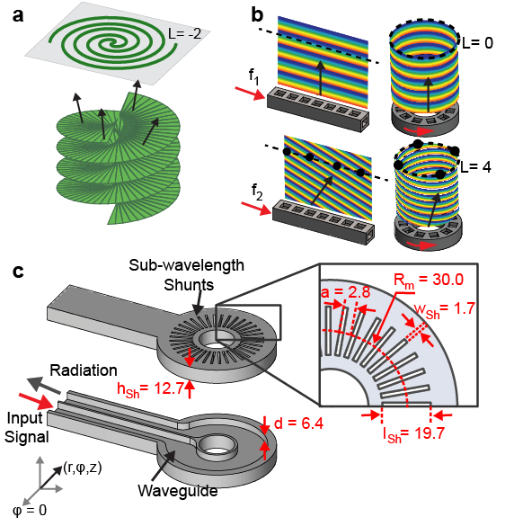
Figure 1: Schematic of acoustic vortex wave antenna: (a) Illustration of a propagating vortex wave, and the resulting vortex constant phase contours in a plane parallel to the aperture. The arrows correspond to the wavenumber vectors which have both vertical, and radial components. (b) A one-dimensional leaky wave antenna can be converted to a vortex wave antenna by wrapping the waveguide back on itself. At normal incidence, excited by frequency $f_{1}$, the OAM mode is zero, with no helicity. Increasing the input frequency to $f_{2}$ produces an angled wavefront which wraps to a helical vortex beam. (c) Exploded-view drawing of the acoustic vortex wave antenna (all dimensions in mm). The input signal goes through one side of the waveguide and the radiated port is fully absorbing to prevent reflections. Inset: detail of shunt geometry.

The confinement of the waveguide in the radial ($\hat{r}$) and axial($\hat{z}$) directions imposes constraints that determine the dispersion relation as a function of frequency. In order to solve for the dispersion, it is convenient to use a coordinate transformation Chin1998 , $u=b\ln(r/b)$ and $v=b\phi$, that unwraps the circular annulus in cylindrical coordinates $(r,\phi,z)$ to form a linear cartesian waveguide with coordinates $(u,v,z)$. After applying the coordinate transform, the wave equation in the plane formed by the annulus becomes,

$$\frac{\partial^{2}\Psi}{\partial u^{2}}+\frac{\partial^{2}\Psi}{\partial v^{2}}+k^{2}(\omega)\exp(u/b)\left[\exp(u/b)-\frac{i\alpha(\omega)}{k(\omega)b}\right]\Psi=0$$ (2)

where $\Psi(u,v)$ is the acoustic pressure in the polar plane, $b$is a scaling parameter of the transform, $k(\omega)=\omega/c$ is the unconstrained wavenumber in air, and $\alpha(\omega)$ depends on the geometry, impedance, and axial confinement of the waveguide. Further details of the analytic model, which takes into account the cumulative end corrections of all shunts, can be found in the supplementary materials. The solutions to Eq. (2) include a phase term $\exp(iL\phi)$, where the topological mode $L$ is fixed by the radial and axial boundary conditions and is radially independent, advancing the phase uniformly at all radii inside the waveguide. We emphasize that $L$ does not depend on the choice of $b$; the physics of the propagation around the annulus cannot change with the scale of the transformation. The utility of the scaling parameter $b$ is to determine both the dispersion relation $\beta(b,\omega)=L(\omega)/b$ and the radiation angle $\theta(b,\omega)=\arcsin[\beta(b,\omega)/k]$ at a particular radius $r=b$ inside the waveguide. Traditionally the scaling parameter $b$ has been chosen to represent the centroid of the radial part of the solution $\Psi(r,\phi)$ Chin1998 ; thus one can define a centroid propagation angle based onthis choice. For a given geometry, $L$ is spatially independent and only depends on frequency; the frequency dependence of $L$ can be tuned by changing the confinement geometry of the waveguide (radial or axial) and/or the shunt geometries.

Using the theory described above, a vortex wave antenna geometry was chosen which is capable of generating at least 7 distinct, orthogonal vortex modes. Finite element methods (FEM) were used to predict the OAM phase topology of each mode, and the design geometry was verified by successful experimental demonstration of the radiated mode. The predicted phase profiles at four frequencies corresponding to whole integer modes are shown in Fig. 2(a).

The realized vortex wave antenna was fabricated and characterized. Figure 2(b) shows the measured phase topology of 7 modes, extracted from the measured pressure fields, corresponding to $L=-3$ through $L=+3$. This general design proves extremely versatile. For example, using the same unit cell geometry shown in Fig. 1 and simply changing the aperture’s radial midpoint, $R_{m}$, an entirely new set of mode values are realized. This design flexibility opens the door to vortex beam multiplexing by designing an aperture with multiple concentric waveguides resulting in a multiplexed beam, ideal for high-speed communications applications. Additionally, the versatility of the design space enables tailoring of the aperture radius to be either scaled down even further in size, or increased to minimize vortex beam divergence.

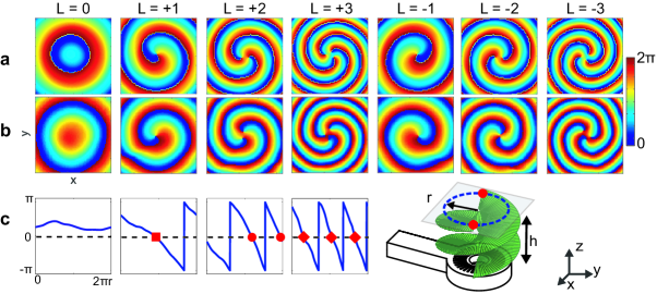
Figure 2: Finite element simulated (a) and measured (b) phase distributions of OAM waves with topological charges ranging from -3 to +3: The various charges were generated using a single metamaterial aperture by insonifying the aperture at discrete frequencies. All measurements were taken at a distance of $h$ from the surface of the antenna, where $h$ 50 mm. The evaluated frequncies are 1.8kHz, 2.8kHz, 4.1kHz and 5.45kHz. (c) The method for determination of mode magnitude consists of counting the number of phase fronts which cross a circle that is co-axial with the aperture. The circle, defined on the measurement plane in (a) and (b), is shown in (c, far right). Phase magnitude, collected from the simulated data in (a), is shown with the number of phase fronts indicated by red symbols.

To quantify the momentum mode number of each mode, the phase of the radiated beam has been mapped onto a circle whose axis is concentric with the antenna axis at $r\!=\!0$. The corkscrew wavefront of the radiated beam carries the OAM of the waveguide’s dispersion, with phase $\exp(iL\phi)$. Thus for a value of $L$, the phase of a vortex beam will cycle $L$ times through $2\pi$ around the circumference of the axis-concentric circle. Figure 2(c) shows the phase of the radiated beam on a circle of radius $r\!=\!0.1$ m.

The phase at each frequency in the band from 1.8 kHz to 6.3 kHz is unwrapped by adding multiples of $2\pi$ at each phase value of -$\pi$ and integrated along a closed path to determine the total change in phase, $\Delta\Phi$, as a function of frequency. The experimentally obtained values of $\Delta\Phi$ are shown as red circles in Fig. 3(a) and are observed to discontinuously jump between integer plateaus. This metric indicates that unlike the predicted continuous monotonic change in the topological mode within the waveguide, the mode numbers of the radiated vortex waves are only observed at discrete integer values. This result, while seemingly paradoxical, is in agreement with previous theoretical and experimental results demonstrated for electromagnetic (EM) vortex waves Vasnetsov1998 ; Berry2004 .

Fractional ordering of the topological modes can instead be observed in the vorticity structure of the radiated beam Berry2004 . Integer modes have no phase discontinuity around the annulus (see Fig. 2(b))and are expected to produce a single radiated vortex, with an accompanying null in amplitude (see Fig. 4(a)), that is centered on the beam’s axis. Fractional modes, on the other hand, result in multiple observed vortices, with associated nulls in amplitude, centered around the beam axis Berry2004 . The number of vortices arising from a fractional topology is given by the closest integer to $L$, and are predicted to increase discontinuously when $L\!=\!N+1/2$, where $N$ is an integer.

As the phase approaches a half-mode, a radially-oriented line of vortex pairs (and associated nulls) appears in the radiated beam profile Berry2004 ; Vasnetsov1998 . This pattern can be observed in the measured phase and amplitude profiles as a dislocation in the wavefront, shown in Fig. 3(b) for $L\!=\!-1.5$ and $L\!=\!-3.5$ at frequencies where the unwrapped phase is observed to transition between integer modes. The introduction of these fractional modes can be seen in the supplementary material. Since these vortex pairs are equal in magnitude but have opposite signs, summation along a closed path leads to no net contribution to the total vorticity. As the value of $L$ increases beyond a half integer, one of these line vortices breaks off to to form the next higher integer vortex singularity in the cluster, while the others disappear Berry2004 . It has been theoretically predicted that in free space this should lead to a rapid jump from one integer mode to the next, which is in excellent agreement with the observed experimental results obtained using the unwrapped-phase metric presented in Fig. 3(a). This fractional effect, in which a dislocation in the wavefront appears, has also been described as an analog to the Aharonov-Bohm effect with a flux line consisting of wavefronts along a nodal surface.Berry2004 ; Berry1980

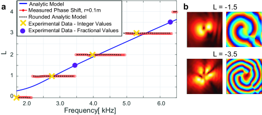
Figure 3: Comparison of calculated and measured modes (a), and measured fractional modes (b): (a) Calculated mode value (blue lines). Integer values of L were chosen from the experimental emitted spectrum of the aperture. Measured integer modes are indicated as discrete yellow x-marks, while fractional values are indicated as filled circles. The horizontal lines correspond to (red) the measured mode number determined by phase unwrapping, (black-dashed) theory rounded to the nearest integer, consistent with mode determination set up by BerryBerry2004 . (b) Measured pressure (left) and phase (right) amplitudes at frequencies representing fractional vortex values of -1.5 and -3.5.

Inspection of the amplitude nulls in Fig. 4(a) indicates that multiple vortex singularities are also present at the frequencies which predict integer values for the cases of $L=\pm 2$ and $\pm 3$. Finite element simulation indicates that this apparent fractional topology is a result of the aperture design, where the input and output ports cause the design to be missing a wedge compared to a perfect circle. The missing wedge acts as an effective phase discontinuity at the aperture, which produces a beam profile that appears to result from a fractional phase dispersion. With an ideal design in which the input and output ports are removed and a continuity condition placed on the wrapped waveguide, perfect integer modes would be achievable. We emphasize that the ideal vortex wave antenna concept (with continuity condition) is capable of generating not only whole integer modes, but fractional vortex modes as well (observed in Fig. 3(b)), which have found a myriad of uses in their own right.

Since mode orthogonality is vital for many applications of vortex waves including high-speed communications and imaging, the covariance matrix of the measured modes was calculated. Figure 4(a) shows the measured intensity ($\|p\|^{2}$) distributions for the $L=0$, $\pm 1$, $\pm 2$, and $\pm 3$ modes. The covariance matrix of the measured modes is plotted in Fig. 4(b). The details of the calculation can be found in the supplementary materials. The covariance matrix shows that despite the lack of symmetry in the mode shapes, each mode distribution is highly uncorrelated with the others, indicating a high degree of orthogonality.

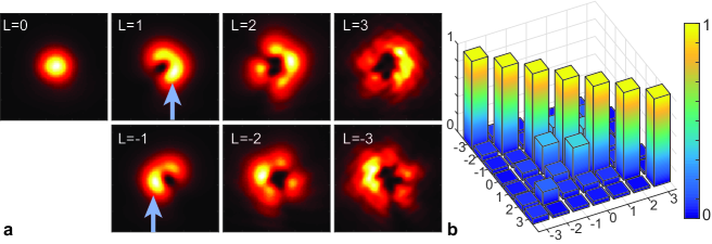
Figure 4: Measured mode intensities and calculated orthogonality: (a) Measured acoustic intensity plots of $L=0$, $\pm 1$, $\pm 2$, and $\pm 3$ modes measured respectively at frequencies 1.8kHz, 2.8kHz, 4.1kHz and 5.45kHz. Arrow indicates input port direction for the top and bottom rows. (b) Symmetric mode orthogonality matrix for all $L$ modes shown in (a).

Our acoustic vortex wave antenna approach offers an extremely compact method to emit vortex modes with the diameter of the aperture being the size of the wavelength of excitation at the highest frequency examined. The small, electronically and geometrically simple device makes this vortex wave antenna ideal for both scaling, and for integration into systems requiring a large number of vortex beams. Acoustic OAM waves have already shown usefulness in micromanipulation, such as an acoustic tractor beam, and for fluid mixing. Although these concepts can be also achieved using optical vortex beams, acoustic particle manipulation has advantages over optical manipulation in that it gives the ability to manipulate both larger objects and non-magnetic or non-conducting materialsDing2012 ; Mulvana2013 .

Author Contributions

C.N. conceived the idea and designed the aperture. C.R. and M.N. collected the experimental data and performed the data analysis. T. M. and M. G. derived the analytical transformation calculation. G.O. provided guidance on the research direction and the applications. All authors contributed to writing the paper.

Competing Financial Interests

The authors declare no competing financial interests.

Supplementary Material

I Materials and Methods

Finite element simulations (FEM) of the vortex wave were performed using COMSOL multiphysics. The FEM used a circular waveguide with geometry indicated. The boundary conditions on the waveguide were rigid in the radial direction and a continuous radiation condition was imposed on the exit port of the waveguide. In order to be consistent with the geometry realized experimentally, a wedge of the waveguide was removed corresponding to the input and output ports in the fabricated system. The circular waveguide aperture is fed via the input port using an omnidirectional source. This was simulated in the finite element model using a source signal in the form of a continuous wave at constant amplitude. Perfect absorbing conditions were mandated at the exit port of the waveguide to prevent reflection. Mode chirality was tuned by switching the location of the source between input and output ports.

The leaky wave aperture was fabricated using additive manufacturing in two pieces as indicated in Figure 1. The dimensions were chosen to provide an antenna which would have the best performance at the frequencies for which the transducers had optimal performance. Soft putty was used to seal the top and bottom plates and prevent sound leakage. The aperture design incorporates an input/output waveguide. The omnidirectional sound source was coupled into this waveguide using a 1 m long pipe in order to mitigate the effects of reflection. The output port was filled with sound-absorbing foam. The source profile was an linear frequency modulated (LFM, or chirped) pulse. The LFM pulse was 6ms in duration and windowed with a Hanning envelope function. The LFM pulse was a linear ramp of frequencies from 1kHz to 10kHz (generated with the MATLAB chirp and hann functions). This waveform was digitized with a Agilent 33220A waveform generator and fed to a Dayton Audio CE32A-8 speaker. Efforts were made to mitigate reflection in the radiation area by using anechoic foam. A microphone (Breül and Kjær 4939-A) mounted on an automated two-dimensional positioning system was used to map the emitted intensity and phase profile above the aperture. Multiple 10ms long waveforms were collected and averaged together to fully capture the 6ms LFM, accounting for waveguide dispersion and collection time of flight. As in the simulated result, chirality was varied by switching input and output ports. In all predicted and measured phase and intensity plots the aperture is centered on in the image. The phase and intensity profiles are mapped at a plane parallel to the surface of the aperture over an area of 0.16 m² square and at a height of 0.05 m from the top of the aperture.

II Vortex Leaky Wave Antenna: Analytic Model

II.1 Introduction

The circular acoustic leaky wave antenna (LWA) is designed using a ring antenna architecture in cylindrical coordinates. Our design assumes propagation around an annular ring in the azimuthal $\hat{\phi}$ direction, with waveguide confinement in the radial $\hat{r}$ and axial $\hat{z}$ directions. There are quasi-radiating boundaries at the input/output ports of the ring (Fig. 1(C) of the main text) that allow an acoustic wave to adiabatically enter and leave the circular waveguide with minimal reflection (to first order). Therefore, for purposes of an analytic approximation we assume no confinement in the azimuthal direction. The wave equation in cylindrical coordinates is,

$$\frac{1}{r}\frac{\partial}{\partial r}\left(r\frac{\partial P}{\partial r}\right)+\frac{1}{r^{2}}\frac{\partial^{2}P}{\partial\phi^{2}}+\frac{\partial^{2}P}{\partial z^{2}}+k^{2}P=0$$ (3)

where $P(r,\phi,z)$ is the acoustic pressure and $k=\omega/c_{0}$ is the wavenumber in air. We assume an acoustic wave of the form $\tilde{P}\exp(i\omega t-i\vec{k}\vec{\cdot x})$ such that a negative imaginary wavenumber results in loss. The annular waveguide has acoustic shunts in its upper axial plane that allow the acoustic wave to radiate in the positive $\hat{z}$ direction. The shunts have rectangular cross-section but are aligned along the radial direction and have a constant azimuthal spacing $\phi_{a}$. The dimensions of the acoustic shunts and waveguide are given in Table I.

Parameter	Value (mm)	Description
$l_{Sh}$	19.7	Shunt length in $\hat{r}$ direction
$w_{Sh}$	1.7	Shunt width in $\hat{\phi}$ direction
$h_{Sh}$	12.7	Shunt depth in $\hat{z}$ direction
$R_{i}$	17.3	Inner radius of Shunt/Waveguide
$R_{o}$	42.7	Outer radius of Shunt/Waveguide
$R_{m}$	30.0	Midpoint radius of Shunt/Waveguide
$d$	6.5	Waveguide height in $\hat{z}$ direction
$a$	6.7	Shunt spacing at $R_{o}$ in $\hat{\phi}$ direction

Table 1: Dimensions of the leaky wave antenna.

The waveguide’s cross-sectional dimensions are smaller than the acoustic wavelength $\lambda\simeq 43$ mm at the highest experimental frequency of 8 kHz. Therefore we expect a single propagating mode, confined in the $\hat{r}$ and $\hat{z}$ directions, that traverses the circular LWA in the $\hat{\phi}$ direction. The LWA will radiate a vortex wave that is dependent on the topological charge $L(\omega)$, which indexes the orbital angular momentum of the waveguide’s azimuthal mode. One must solve Eq. 3 under the confinement constraints of the waveguide in order to estimate the frequency dependence of the topological charge.

II.2 Solutions to the Cartesian Coordinate Transform

To solve for the dispersion relation of the annular propagation, we employ a coordinate transformation that has been successfully applied to electromagnetic ring resonators Chin1998 , $u=b\ln(r/b)$ and $v=b\phi$, with $z$ unchanged. Here $b$ is a scaling parameter that has units of radius. The transformation maps the cylindrical annulus to a linear cartesian waveguide with coordinates $\left(u,v,z\right)$. Under this coordinate transformation the wave equation becomes,

$$\frac{\partial^{2}P}{\partial u^{2}}+\frac{\partial^{2}P}{\partial v^{2}}+\exp(2u/b)\frac{\partial^{2}P}{\partial z^{2}}+k^{2}\exp(2u/b)P=0.$$ (4)

Using separation of variables $P(u,v,z)=F(u,z)G(v)$ we assign a plane wave solution $G(v)=C\exp(i\beta v)+D\exp(-i\beta v)$ to describe the propagation along the (transformed) linear waveguide, where the propagation constant $\beta$ defines the radiation angle in the transformed system. The wave equation now becomes,

$$\frac{\partial^{2}F}{\partial u^{2}}+\exp(2u/b)\frac{\partial^{2}F}{\partial z^{2}}+\left[k^{2}\exp(2u/b)-\beta^{2}\right]F=0.$$ (5)

An exact solution $F(u,z)$ to Eq. 5 is not separable due to the radial dependence of our shunt geometry; however, one can exploit the subwavelength scale of the axial confinement to derive an approximate solution that is separable. We assume that $F(u,z)=\psi(u)\chi(z)$ with $\chi(z)=B\cos\left(\gamma z\right)$ under the condition that $\gamma d\ll 1$. Note that $d$ is the maximal value of $z$ in the waveguide and the rigid lower boundary is placed at $z=0$. Under this assumption the confinement parameter $\gamma$ can be written as,

$$\gamma\simeq\sqrt{\frac{ikw_{Sh}}{\phi_{a}d}\frac{Z_{0}}{Z_{Sh}(\omega)}\frac{1}{b\exp(u/b)}},$$ (6)

which can be derived from the impedance boundary condition of the shunts at the axial upper boundary ($z=d$). Here $Z_{Sh}(\omega)$ is the acoustic impedance of an individual shunt and $Z_{0}$ is the impedance of air. Although $\gamma$ depends explicitly on $u$, it is easy to show that the non-separable terms in Eq. 5 are proportional to $(\gamma z)^{2}$ and are therefore negligible in the limit $\gamma d\ll 1$. In this limit the wave equation can be written as,

$$\frac{\partial^{2}\psi}{\partial u^{2}}+\left\{k^{2}\exp(u/b)\left[\exp(u/b)-\frac{i\alpha(\omega)}{kb}\right]-\beta^{2}\right\}\psi=0,$$ (7)

$$\alpha(\omega)=\frac{w_{Sh}}{\phi_{a}d}\frac{Z_{0}}{Z_{Sh}(\omega)}.$$ (8)

After applying rigid boundary conditions at $u_{i}(R_{i})$ and $u_{o}(R_{o})$, and transforming back to cylindrical coordinates, the solution to Eq. 7 in the plane of the ring is,

$$\Psi(r,\phi)=\psi(r)G(\phi)=A\,r^{L}\exp[\pm iL\phi-ikr]\left(\Omega[\mu,2L+1,2ikr]+\xi\Lambda[-\mu,2L,2ikr]\right),$$ (9)

$$\mu=\left(2L+1+\alpha\right)/2,$$ (10)

where $\Omega[\mu,2L+1,2ikr]$ is the confluent hypergeometric function, $\Lambda[-\mu,2L,2ikr]=\Lambda_{-\mu}^{2L}(2ikr)$ is the generalized Laguerre polynomial, and $L=\beta b$ is the topological charge. The parameter $\xi$ defines the proportionality between $\Omega[...]$ and $\Lambda[...]$, is $L$-dependent but spatially independent, and is derived from the radial boundary conditions. The topological charge $L$ is invariant under the choice of $b$, and is spatially independent for a given waveguide geometry. $L$ indexes the azimuthal phase in the same manner as the Bessel order in the solution to the unconfined cylindrical wave equation, except that here $L$ can take on non-integer values.

II.3 Impedance of the shunts

The acoustic impedance of each shunt is determined from the dynamic mass response of its internal air column, viscous end corrections at the openings, and mass end corrections due to radiation from the shunt and its neighbors. The internal mass response is proportional to the shunt depth $h_{Sh}$ Chocano2015 ,

$$Z_{h}=i\omega\rho_{0}h_{Sh}\left[1-\frac{\tanh(s\sqrt{i})}{s\sqrt{i}}\right]^{-1}$$ (11)

$$s=w_{Sh}\sqrt{\frac{\omega\rho_{0}}{\eta_{0}}}$$ (12)

where $\eta_{0}$ is the dynamic viscosity of air. The viscous and mass end corrections are discussed at length by Ingard Ingard1953 . The viscous end correction can be approximated as Chocano2015 ; Ingard1953 ,

$$Z_{v}=\sqrt{8\eta_{0}\omega\rho_{0}}.$$ (13)

The mass end corrections $Z_{e,i}$ can be calculated using a double integration over the cross-sectional area of the shunt and its neighbors Temkin2001 ,

$$Z_{e,i}\simeq\frac{i\omega\rho_{0}}{2\pi l_{Sh}w_{Sh}}\int_{A}\int_{A^{\prime}}\frac{e^{ikR^{\prime}}}{R^{\prime}}dA^{\prime}dA$$ (14)

where $Z_{e}$ and $Z_{i}$ are impedance corrections at the external and internal ends of the shunt, respectively. Here $dA$ is an infinitesimal area element of the shunt’s cross-section, $dA^{\prime}$ is a cross-sectional area element of the shunt or its neighboring shunts, and $R^{\prime}$ is the displacement between elements $dA$ and $dA^{\prime}$ Temkin2001 . The total shunt impedance is then the series combination of each component, $Z_{Sh}=Z_{h}+Z_{v}+Z_{e}+Z_{i}$.

The double integral in Eq. 14 is intractable for a rectangular cross-section, and series approximations have been carried out by Ingard Ingard1953 . We use numerical integration to estimate $Z_{e,i}$, where the integration is carried out over all 35 shunts for the external end correction while the internal correction includes only the nearest and second-nearest neighboring shunts. The integral in Eq. 14 is multiplied by a phasing function $\exp(i\Phi)$ for each neighbor that approximates the phase change around the ring, where the value of $\Phi$ is estimated from the measured topological charge at a given frequency. Additionally, mirror reflections from the rigid boundaries inside the waveguide will result in virtual neighbors; we include the first set of these virtual neighbors (one above $R_{o}$ and one below $R_{i}$) in the estimate of the internal end correction.

As the curvature of the waveguide grows, direct displacement vectors between shunts inside the waveguide will become disrupted by the waveguide’s walls, resulting in displacement vectors involving multiple reflections. Given that the displacement $R^{\prime}$ for reflected vectors is highly sensitive to the wall curvature, and that the phase $\Phi$ is not constant around the ring, we assume that the contributions of multiple internal reflections from distant neighbors will largely cancel out. Therefore, there is some amount of error in choosing the number of shunts to include in the calculation of the internal end correction. The near field corrections due to neighboring shunts become stronger at lower frequencies, approaching a magnitude similar to $Z_{h}$ at frequencies below $L=1$; therefore the uncertainty is strongest at these frequencies.

III Calculation of Spatial Mode Orthogonality

The following procedure was used to compute the spatial mode covariance matrix. This is a measure of the spatial mode orthogonality. The norm of each mode, $N_{m}$, was computed using the Fourier transformed pressure time series data, $p({\bf{x}},t)$Tao2014 :

$$\int_{\Omega}P_{m}({\bf{x}},f)P_{m}^{*}({\bf{x}},f)d\Omega\equiv N_{m}$$ (15)

where $P_{m}$ is the Fourier transform of the collected time series data, the mode number $m=-3,-2,-1,0,+1,+2,+3$ was selected at discrete frequencies, $f$, guided by the spiral wave condition $m=2\pi\beta r$ of Fig. 3 in the main text. $\Omega$ is the sample plane of the mode distribution, and $P^{*}$ indicates complex conjugation. The covariance between two separate modes, $m$, and $n$ is given by:

$$C_{mn}=\int_{\Omega}\frac{1}{\sqrt{N_{m}}}P_{m}({\bf{x}},f)\frac{1}{\sqrt{N_{n}}}P^{*}_{n}({\bf{x}},f)d\Omega$$ (16)

and were approximated with the discrete formulation:

$$\textrm{C}_{mn}\simeq\frac{1}{M}\sum_{j=1}^{M}\frac{1}{\sqrt{N_{m}}}P_{m}({{x}_{j}},f)\frac{1}{\sqrt{N_{n}}}P^{*}_{n}({{x}_{j}},f)$$ (17)

with $j$ indexing each position in the collected sample planes. A discrete Fourier transform was used to calculate the complex frequency domain pressure amplitudes and phases. Sufficient padding was added to the 7ms, Tukey windowed time series data sets to create a $\Delta f=25$Hz. The full results of the pressure and phase evolution as a function of frequency can be found in the animations included in the supplementary materials.

References

- (1) B. T. Hefner and P. L. Marston, “An acoustical helicoidal wave transducer with applications for the aligntment of ultrasonic and underwater systems,” J. Acoust. Soc. Am., vol. 106, p. 3313, 1999.
- (2) C. Wilson and M. J. Padgett, “A polyphonic acoustic vortex and its complementary chords,” New J. Phys., vol. 12, p. 023018, 2010.
- (3) A. Marzo, S. A. Seah, B. W. Drinkwater, D. R. Sahoo, B. Long, and S. Subramanian, “Holographic acoustic elements for manipulation of levitated objects,” Nat. Commun., vol. 6, p. 8661, 2015.
- (4) A. Riaud, J.-L. Thomas, E. Charron, A. Bussonniere, O. B. Matar, and M. Baudoin, “Anisotropic swirling surface acoustic waves from inverse filtering for on-chip generation of acoustic vortices,” Phys. Rev. App., vol. 4, p. 034004, 2015.
- (5) R. Wunenburger, J. I. V. Lozano, and E. Brasselet, “Acoustic orbital angular momentum transfer to matter by chiral scattering,” New J. Phys., vol. 17, p. 103022, 2015.
- (6) E. Karimi, S. A. Shultz, I. DeLeon, H. Qassim, J. Upham, and R. W. Boyd, “Generating optical angular momentum at visible wavelengths using a plasmonic metasurface,” Light Science and Applications, vol. 3, p. e167, 2014.
- (7) B. J. McMorran, A. Agrawal, I. M. Anderson, A. A. Herzing, H. J. Lezec, J. J. McClelland, and J. Unguris, “Electron vortex beams with high quanta of orbital angular momentum,” Science, vol. 331, pp. 192–195, 2011.
- (8) C. J. Naify, M. D. Guild, C. A. Rohde, D. C. Calvo, and G. J. Orris, “Demonstration of a directional sonic prism in two dimensions using an air-acoustic leaky wave antenna,” Appl. Phys. Lett., vol. 107, no. 13, p. 133505, 2015.
- (9) A. Malr, A. Vazlri, G. Wehls, and A. Zellinger, “Entanglement of the orbital angular mometnum states of photons,” Nature, vol. 412, pp. 313–316, 2001.
- (10) G. Molina-Terriza, J. P. Torres, and L. Torner, “Twisted photons,” Nat. Phys., vol. 3, pp. 305–310, 2007.
- (11) M. J. Strain, X. Cai, J. Wang, J. Zhu, D. B. Phillips, L. Chen, M. Lopez-Garcia, J. L. O’Brien, M. G. Thompson, M. Sorel, and S. Yu, “Fast electrical switching of orbital angular mometum modes using ultra-compact integrated vortex emitters,” Nat. Coomun., vol. 5, no. 4856, 2014.
- (12) A. Willner, H. Huang, Y. Yan, Y. Ren, N. Ahmed, G. Xie, C. Bao, L. Li, Y. Cao, Z. Zhao, J. Wang, M. Lavery, M. Tur, S. Ramachandran, A. F. Molisch, N. Ashcrafi, and S. Ashrafi, “Optical communications using orbital angular momentum beams,” Adv. Opt. Photon., vol. 7, pp. 66–106, 2015.
- (13) J. Harris, V. Grillo, E. Mafakheri, G. C. Gazzadi, S. Frabboni, F. W. Boyd, and E. Karimi, “Structured quantum waves,” Nat. Phys., vol. 11, pp. 629–634, 2015.
- (14) A. Jesacher, S. Furhapter, S. Bernet, and M. Ritsch-Marte, “Shadow effects in spiral phase contrast microscopy,” Phys. Rev. Lett., vol. 94, no. 23, p. 233902, 2005.
- (15) S. Bernet, A. Jesacher, S. Furhapter, C. Maurer, and M. Ritsch-Marte, “Quantitative imaging of complex samples by spiral phase contrast microscopy,” Opt. Express, vol. 14, pp. 3792–3805, 2006.
- (16) L. Chen, J. Lei, and J. Romero, “Quantum digital spiral imaging,” Light Science and Applications, vol. 3, no. e153, 2014.
- (17) D. G. Grier, “A revolution in optical manipulation,” Nature, vol. 424, p. 810, 2003.
- (18) K. Ladavac and D. G. Grier, “Microoptomechanical pumps assembled and driven by holographic optical vortex arrays,” Opt. Express, vol. 12, no. 6, pp. 1144–1149, 2004.
- (19) Z. Y. Hong, J. Zhang, and B. W. Drinkwater, “Observatin of orbital angular momentum transfer from bessel-shaped acoustic vortices to diphasic liquid-microparticle mixtures,” Phys. Rev. Lett., vol. 114, p. 214301, 2015.
- (20) X. Cai, J. Wang, M. J. Strain, M. Johsnon-Morris, J. Zhu, M. Sorel, J. L. O’brien, M. G. Thompson, and S. Yu, “Integrated compact optical vortex beam emitters,” Science, vol. 338, pp. 363–366, 2012.
- (21) Z. Hong, J. Zhang, and B. W. Drinkwater, “On the radiation force fields of fractional-order acoustic vortices,” EPL, vol. 110, p. 14002, 2015.
- (22) J. Wang, W. Zhang, Q. Qi, S. Zheng, and L. Chen, “Gradual edge enhancement in spiral phase contrast imaging with fractional vortex filters,” Scientific Reports, vol. 5, pp. 15826 EP –, 10 2015.
- (23) C. J. Naify, T. P. Martin, M. Nicholas, D. C. Calvo, and G. J. Orris, “Experimental realization of a variable index transmission line metamaterial as an acoustic leaky-wave antenna,” Appl. Phys. Lett., vol. 102, no. 4, p. 203508, 2013.
- (24) L. Liu, C. Caloz, and T. Itoh, “Dominant mode leaky-wave antenna with backfire-to-endfire scanning capability,” Electronics Letters, vol. 38, no. 23, p. 1414, 2002.
- (25) M. K. Chin and S. T. Ho, “Design and modeling of waveguide-coupled single-mode microring resonators,” J. Lightwave Technol., vol. 16, no. 8, p. 1433, 1998.
- (26) M. V. Vasnetsov, L. V. Bastisty, and M. Soskin, “Free-space evolution of monochromatic mixed screw-edge wavefront dislocations,” Proc. SPIE, vol. 3487, pp. 29–33, 1998.
- (27) M. V. Berry, “Optical vortices evolving from helicoidal integer and fractional phase steps,” J. Opt. A: Pure Appl. Opt., vol. 6, pp. 259–268, 2004.
- (28) M. V. Berry, R. G. Chambers, M. D. Large, C. Upstill, and J. C. Walmsley, “Wavefront dislocations in the aharonov-bohm effect and its water wave analog,” Eur. J. Phys., vol. 1, pp. 154–162, 1980.
- (29) X. Ding, S.-C. S. Lin, B. Kiraly, H. Yue, S. Li, I.-K. Chiang, J. Shi, S. J. Benevic, and T. J. Huang, “On-chip manipulation of single microparticles, cells and organizms using surface acoustic waves,” Proc. Natl. Acad. Sci. U.S.A., vol. 109, no. 28, pp. 11105–11109, 2012.
- (30) H. Mulvana, S. Cochran, and M. Hill, “Ultrasound assited partical and cell manipulation on-chip,” Adv. Drug Deliv. Rev., vol. 65, pp. 1600–1610, 2013.
- (31) M. K. Chin and S. T. Ho, “Design and modeling of waveguide-coupled single-mode microring resonators,” J. Lightwave Technol., vol. 16, no. 8, p. 1433, 1998.
- (32) V. M. G. Chocano, “New devices for noise control and acoustic cloaking,” 2015.
- (33) U. Ingard, “On the theory and design of acoustic resonators,” J. Acoust. Soc. Am., vol. 25, no. 6, p. 1037, 1953.
- (34) S. Temkin, Elements of Acoustics. U.S.A.: Acoustical Society of America, 2001.
- (35) Z.-Y. Tao and Y.-X. Fan, “Orthgonality breaking induces extraordinary single-mode transparence in an elaborate waveguide with wall corrugationgs,” Sci. Reports, vol. 4, p. 7092, 2014.