1–LABEL:LastPageFeb. 22, 2017May 09, 2018 \savesymboliint \savesymboliiint
Analyzing Timed Systems Using Tree Automata
Abstract.
Timed systems, such as timed automata, are usually analyzed using their operational semantics on timed words. The classical region abstraction for timed automata reduces them to (untimed) finite state automata with the same time-abstract properties, such as state reachability. We propose a new technique to analyze such timed systems using finite tree automata instead of finite word automata. The main idea is to consider timed behaviors as graphs with matching edges capturing timing constraints. When a family of graphs has bounded tree-width, they can be interpreted in trees and MSO-definable properties of such graphs can be checked using tree automata. The technique is quite general and applies to many timed systems. In this paper, as an example, we develop the technique on timed pushdown systems, which have recently received considerable attention. Further, we also demonstrate how we can use it on timed automata and timed multi-stack pushdown systems (with boundedness restrictions).
Key words and phrases:
Timed automata, tree automata, pushdown systems, tree-width1991 Mathematics Subject Classification:
F.1.1 Models of Computation1. Introduction
The advent of timed automata [4] marked the beginning of an era in the verification of real-time systems. Today, timed automata form one of the well accepted real-time modelling formalisms, using real-valued variables called clocks to capture time constraints. The decidability of the emptiness problem for timed automata is achieved using the notion of region abstraction. This gives a sound and finite abstraction of an infinite state system, and has paved the way for state-of-the-art tools like UPPAAL [6], which have successfully been used in the verification of several complex timed systems. In recent times [1, 8, 14] there has been a lot of interest in the theory of verification of more complex timed systems enriched with features such as concurrency, communication between components and recursion with single or multiple threads. In most of these approaches, decidability has been obtained by cleverly extending the fundamental idea of region or zone abstractions.
In this paper, we give a technique for analyzing timed systems in general, inspired from a completely different approach based on graphs and tree automata. This approach has been exploited for analyzing various types of untimed systems, e.g., [18, 11]. The basic template of this approach has three steps: (1) capture the behaviors of the system as graphs, (2) show that the class of graphs that are actual behaviors of the system is MSO-definable, and (3) show that this class of graphs has bounded tree-width (or clique-width or split-width), or restrict the analysis to such bounded behaviors. Then, non-emptiness of the given system boils down to the satisfiability of an MSO sentence on graphs of bounded tree-width, which is decidable by Courcelle’s theorem. But, by providing a direct construction of the tree automaton, it is possible to obtain a good complexity for the decision procedure.
We lift this technique to deal with timed systems by abstracting timed word behaviors of timed systems as graphs consisting of untimed words with additional time-constraint edges, called words with timing constraints (TCWs). The main complication here is that a TCW describes an abstract run of the timed system, where the constraints are recorded but not checked. The TCW corresponds to an actual concrete run if and only if it is realizable, i.e., we can find time-stamps realizing the TCW. Thus, we are interested in the class of graphs which are realizable TCWs.
For this class of graphs, the above template tells us that we need to show (i) these graphs have a bounded tree-width and (ii) the property of being a realizable TCW is MSO-definable. Then by Courcelle’s theorem we obtain a tree automaton accepting this. However, as mentioned earlier, the MSO to tree-automaton approach does not give a good complexity in terms of size of the tree automaton. To obtain an optimal complexity, instead of going via Courcelle’s theorem, we directly build a tree automaton. Using tree decompositions of graph behaviours having bounded split/tree-width and constructing tree automata proved to be a very successful technique for the analysis of untimed infinite state systems [18, 12, 11, 2]. This paper opens up this powerful technique for analysis of timed systems.
Thus our contributions are the following. We start by showing that behaviors of timed systems can be written as words with simple timing constraints (), i.e., words where each position has at most one timing constraint (incoming or outgoing) attached to it. This is done by breaking each transition of the timed system into a sequence of “micro-transitions”, so that at each micro-transition, only one timing constraint is attached.
![[Uncaptioned image]](/html/1604.08443/assets/x1.png)
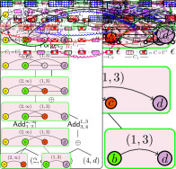
Next, we show that that arise as behaviours of certain classes of timed systems (e.g., timed automata or timed pushdown systems) are graphs of bounded special tree-width. Special tree-width is a graph complexity measure, arising out of a special tree decomposition of a graph, as introduced by Courcelle in [9]. To establish the bound, we play a so-called split-game, which gives a bound on what is called the split-width, a notion that was introduced for graph behaviours of untimed systems and which has proven to be very useful for untimed systems [12, 11, 2]. Establishing a relationship between the split-width and special tree-width, we obtain a bound on special tree-width (which also implies a bound on general tree-width as shown in [9]). As a result of this bound, we infer that our graphs admit binary tree decompositions as depicted in the adjoining figure. Each node of the tree decomposition depicts a partial behaviour of the system in a bounded manner. By combining these behaviours as we go up the tree, we obtain a full behaviour of the system.
Our final and most technically challenging step is to construct tree automata that works on such tree decompositions and accepts only those whose roots are labeled by realizable generated by the timed system . Thus, checking non-emptiness of the timed system reduces to checking non-emptiness for this tree automaton (which is PTIME in the size of the tree automaton). The construction of this tree automaton is done in two phases. First, given the bound on special tree-width of the graph behaviours of , we construct a tree automaton that accepts all such trees whose roots are labeled by realizable with respect to the maximal constant given by the system, and whose nodes are all bounded. For this, we need to check that the graphs at the root are indeed words with valid timing constraints and there exists a time-stamping that realizes the . If we could maintain the partially constructed in a state of the tree automaton along with a guess of the time-stamp at each vertex, we could easily check this. However, the tree automaton has only finitely many states, so while processing the tree bottom-up, we need a finite abstraction of the which remembers only finitely many time values. We show that this is indeed possible by coming up with an abstraction where it is sufficient to remember the modulo values of time stamps, where is one more than the maximal constant that appears in the timed system.
In the second phase, we refine this tree automaton to obtain another tree automaton that only accepts those trees that are generated by the system. Yet again, the difficulty is to ensure correct matching of (i) clock constraints between points where a clock is reset and a constraint is checked, (ii) push and pop transitions by keeping only finite amount of information in the states of the tree automaton. Once both of these are done, the final tree automaton satisfies all our constraints.
To illustrate the technique, we have reproved the decidability of non-emptiness of timed automata and timed pushdown automata (TPDA), by showing that both these models have a split-width ( and ) that is linear in the number of clocks, , of the given timed system. This bound directly tells us the amount of information that we need to maintain in the construction of the tree automata. For TPDA we obtain an ExpTime algorithm, matching the known lower-bound for the emptiness problem of TPDA [1]. For timed automata, since the split-trees are word-like (at each binary node, one subtree is small) we may use word automata instead of tree automata, reducing the complexity from ExpTime to PSpace, again matching the lower-bound [4]. Interestingly, if one considers TPDA with no explicit clocks, but the stack is timed, then the split-width is a constant, 2. In this case, we have a polynomial time procedure to decide emptiness, assuming a unary encoding of constants in the system. To further demonstrate the power of our technique, we derive a new decidability result for non-emptiness of timed multi-stack pushdown automata under bounded rounds, by showing that the split-width of this model is again linear in the number of clocks, stacks and rounds. Exploring decidable subclasses of untimed multi-stack pushdown systems is a very active research area [5, 13, 16, 15, 17], and our technique can extend these to handle time.
It should be noticed that the tree automaton used to check emptiness of the timed system is essentially the intersection of two tree automata. The tree automaton for validity/realizability (Section 4), by far the most involved construction, is independent of the timed system under study. The second tree automaton depends on the system and is rather easy to construct (Section 5). Hence, to apply the technique to other systems, one only needs to prove the bound on split-width and to show that their runs can be captured by tree automata. This is a major difference compared to many existing techniques for timed systems which are highly system dependent. For instance, for the well-established models of TPDA, that we considered above, in [7, 1] it is shown that the basic problem of checking emptiness is decidable (and -complete) by re-adapting the technique of region abstraction each time (and possibly untiming the stack) to obtain an untimed pushdown automaton. Finally, an orthogonal approach to deal with timed systems was developed in [8], where the authors show the decidability of the non-emptiness problem for a class of timed pushdown automata by reasoning about sets with timed-atoms.
An extended abstract of this paper was presented in [3]. There are however, significant differences from that version as we detail now. First, the technique used to prove the main theorem of building a tree automaton to check realizability is completely different. In [3], we showed an automaton which checks for non-existence of negative weight cycles (which implies the existence of a realizable time-stamping). This required a rather complicated proof to show that the constants can be bounded. In fact, we first build an infinite state tree automaton and then show that we can get a finite state abstraction for it. In contrast, our proof in this article directly builds a tree automaton that checks for existence of time-stamps realizing a run. This allows us to improve the complexity and also gives a less involved proof. Second, we complete the proof details and compute the complexity for tree automata for multistack pushdown systems with bounded round restriction, which was announced in [3]. All sketches from the earlier version have been replaced and enhanced by rigorous proofs in this article. Further, several supporting examples and intuitive explanations have been added throughout to aid in understanding.
2. Graphs for behaviors of timed systems
We fix an alphabet and use to denote where is the silent action. For a non-negative integer , we also fix , to be a finite set of closed intervals whose endpoints are integers between and , and which contains the special interval . When is irrelevant or clear from the context, we just write instead of . Further, for an interval , we will sometimes use to denote its upper/right end-point and to denote its lower/left end-point. For a set , we use to denote a partial or total order on . For any , we write if and , and if and there does not exist such that .
2.1. Preliminaries: Timed words and timed (pushdown) automata
An -timed word is a sequence with and is a non-decreasing sequence of real time values. If for all , then is a timed word. The projection on of an -timed word is the timed word obtained by removing -labelled positions. We define the two basic system models that we consider in this article.
Dense-timed pushdown automata (TPDA), introduced in [1], are an extension of timed automata [4], and operate on a finite set of real-valued clocks and a stack which holds symbols with their ages. The age of a symbol in the stack represents time elapsed since it was pushed on to the stack. Formally, a TPDA is a tuple where is a finite set of states, is the initial state, , , are respectively a finite set of input, stack symbols, is a finite set of transitions, is a finite set of real-valued variables called clocks, are final states. A transition is a tuple where , , is a finite conjunction of atomic formulae of the kind for and , are the clocks reset, is one of the following stack operations:
-
(1)
does not change the contents of the stack,
-
(2)
where is a push operation that adds on top of the stack, with age 0.
-
(3)
where is a stack symbol and is an interval, is a pop operation that removes the top most symbol of the stack if it is a with age in the interval .
Timed automata (TA) can be seen as TPDA using operations only. This definition of TPDA is equivalent to the one in [1], but allows checking conjunctive constraints and stack operations together. In [8], it is shown that TPDA of [1] are expressively equivalent to timed automata with an untimed stack. Nevertheless, our technique is oblivious to whether the stack is timed or not, hence we focus on the syntactically more succinct model of TPDA with timed stacks and get good complexity bounds.
The operational semantics of TPDA and TA can be given in terms of timed words and we refer to [1] for the formal definition. Instead, we are interested in an alternate yet equivalent semantics for TPDA using graphs with timing constraints, that we define next.
2.2. Abstractions of timed behaviors as graphs
Definition \thethm.
A word with timing constraints () over is a structure where is a finite set of positions (also refered to as vertices or points), labels each position, the reflexive transitive closure is a total order on and is the successor relation, gives the pairs of positions carrying a timing constraint associated with the interval .
For any position , the indegree (resp. outdegree) of is the number of positions such that (resp. ). A is simple (denoted ) if each position has at most one timing constraint (incoming or outgoing) attached to it, i.e., for all , indegree() + outdegree() 1. A is depicted below with positions labelled over . indegree(4)=1, outdegree(1)=1 and indegree(3)=0. The curved edges decorated with intervals connect the positions related by , while straight edges are the successor relation . Note that this is simple.
![[Uncaptioned image]](/html/1604.08443/assets/x2.png)
Consider a with . A timed word is a realization of if it is the projection on of an -timed word such that for all . In other words, a is realizable if there exists a timed word which is a realization of . For example, the timed word is a realization of the depicted above, while is not.
2.3. Semantics of TPDA (and TA) as simple
We define the semantics in terms of simple . An is said to be generated or accepted by a TPDA if there is an accepting abstract run of such that, and
-
•
the sequence of push-pop operations is well-nested: in each prefix with , number of pops is at most number of pushes, and in the full sequence , they are equal.
-
•
We have with for . Each transition gives rise to a sequence of consecutive points in the . The transition is simulated by a sequence of “micro-transitions” as depicted below (left) and it represents an shown below (right). Incoming red edges check guards from (wrt different clocks) while outgoing green edges depict resets from that will be checked later. Further, the outgoing edge on the central node labeled represents a push operation on stack. Finally, the blue labeled edge denotes a -delay constraint as explained below.
![[Uncaptioned image]](/html/1604.08443/assets/x3.png)
![[Uncaptioned image]](/html/1604.08443/assets/x4.png)
where are conjunctions of atomic clock constraints and are resets. The first and last micro-transitions, corresponding to the reset of a new clock and checking of constraint ensure that all micro-transitions in the sequence occur simultaneously. We have a point in for each micro-transition (excluding the -micro-transitions between ). Hence, consists of a sequence where is the number of timing constraints corresponding to clocks reset during transition and checked afterwards. Thus, the reset-loop on a clock is fired as many times (0 or more) as a constraint is checked on this clock until its next reset. This ensures that the remains simple. Similarly, is the number of timing constraints checked in . We have and all other points are labelled . The set encodes the initial resets of clocks that will be checked before being reset. So we let and is
-
•
for each , the relation for timing constraints can be partitioned as where
-
–
and .
-
–
We have if is a push and is the matching pop (same number of pushes and pops in ).
-
–
for each such that the -th conjunct of is and and for , we have for some . Therefore, every point with is the target of a timing constraint. Moreover, every reset point for should be the source of a timing constraint. That is, denoting , we must have for some . Also, for each , the reset points are grouped by clocks (as suggested by the sequence of micro-transitions simulating ): if and for some then . Finally, for each clock, we require that the timing constraints are well-nested: for all and , with , if then .
-
–
We denote by the set of simple generated by and define the language of as the set of timed words that are realizations of generated by , i.e., . Indeed, this is equivalent to defining the language as the set of timed words accepted by , according to a usual operational semantics [1].
The semantics of timed automata (TA) can be obtained from the above discussion by just ignoring the stack components (using operations only). To illustrate these ideas, a simple example of a timed automaton and an that is generated by it is shown in Figure 1.

We now identify some important properties satisfied by generated from a TPDA. Let be a . We say that is well timed w.r.t. a set of clocks and a stack if for each interval , the relation can be partitioned as where
-
the stack relation corresponds to the matching push-pop events, hence it is well-nested: for all and , if then .
-
For each clock , the relation corresponds to the timing constraints for clock and is well-nested: for all and , if are in the same -reset block (i.e., a maximal consecutive sequence of positions in the domain of ), and , then . Each guard should be matched with the closest reset block on its left: for all and , if are not in the same -reset block then (see Figure 2).

It is then easy to check that defined by a TPDA with set of clocks are well-timed for the set of clocks , i.e., satisfy the properties above: (note that we obtain the same for TA by just ignoring the stack edges, i.e., () above)
Lemma \thethm.
Simple defined by a TPDA with set of clocks are well-timed wrt. set of clock , i.e., satisfy properties (T1) and (T2).
Proof.
The first condition () is satisfied by by definition. For (), let and for some clock . If are points in the same -reset block for some , then by construction of , if then which gives well nesting. Similarly, if are points in different -reset blocks, then by definition of , we have . Also, it is clear that the new clock satisfies (). ∎
3. Bounding the width of graph behaviors of timed systems
In this section, we check if the graphs (STCWs) introduced in the previous section have a bounded tree-width. As a first step towards that, we introduce special tree terms () from Courcelle [9] and their semantics as labeled graphs.
3.1. Preliminaries: special tree terms and tree-width
It is known [9] that special tree terms using at most colors (-) define graphs of “special” tree-width at most . Formally, a -labeled graph is a tuple where is the vertex labeling and is the set of edges for each label . Special tree terms form an algebra to define labeled graphs. The syntax of - over is given by
where , and are colors. The semantics of each - is a colored graph where is a -labeled graph and is a partial injective function assigning a vertex of to some colors.
-
•
consists of a single -labeled vertex with color .
-
•
adds a -labeled edge to the vertices colored and (if such vertices exist).
Formally, if then with if and
-
•
removes color from the domain of the color map.
Formally, if then with and for all .
-
•
exchanges the colors and .
Formally, if then with if , if and if .
-
•
Finally, constructs the disjoint union of the two graphs provided they use different colors. This operation is undefined otherwise.
Formally, if for and then . Otherwise, is not a valid .
The special tree-width of a graph is defined as the least such that for some - . See [9] for more details and its relation to tree-width. For , we have successor edges and -edges carrying timing constraints, so we take with . In this paper, we will actually make use of with the following restricted syntax, which are sufficient and make our proofs simpler:
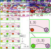
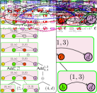
with , , or for some and . The terms defined by this grammar are called -. Here, timing constraints are added directly between leaves in atomic which are then combined using disjoint unions and adding successor edges. For instance, consider the 4- given below
where , stands for The term is depicted as a binary tree on the left of Figure 3 and its semantics is the depicted at the root of the tree in right of Figure 3, where only endpoints labelled and are colored, as the other two colors were “forgotten” by . The entire “split-tree” is depicted in the right of Figure 3 as will be explained in the next sub-section. Abusing notation, we will also use for the graph ignoring the coloring .
3.2. Split-TCWs and split-game
There are many ways to show that a graph (in our case, a simple ) has a bounded special tree-width. We find it convenient to prove that a simple has bounded special tree-width by playing a split-game, whose game positions are simple in which some successor edges have been cut, i.e., are missing. This approach has been used for graph behaviors generated by untimed pushdown systems in [12], but here we wish to apply it to reason about graph behaviors of timed systems. Formally, a split- is a structure where and are the present and absent successor edges (also called holes), respectively, such that and is a . Notice that, for a split-, and . A block or factor of a split- is a maximal set of points of connected by . We denote by the set of left and right endpoints of blocks of . A left endpoint is one for which there is no with . Right endpoints are defined similarly. Points in are called internal. If is any point, denotes the unique block which contains . The number of blocks is the width of : . may be identified with split- of width 1, i.e., with . A split- is atomic if it consists of a single point () or a single timing constraint with a hole (, , ). In what follows, we will use the notation for when convenient.
The split-game is a two player turn based game where Eve’s set of game positions consists of all connected (wrt. ) split- and Adam’s set of game positions consists of all disconnected (wrt. ) split-. The edges of reflect the moves of the players. Eve’s moves consist of splitting a block in two, i.e., removing one successor edge in the graph. Adam’s moves amount to choosing a connected component (wrt. ) of the split-. Atomic split- are terminal positions in the game: neither Eve nor Adam can move from an atomic split-. A play on a split- is a path in starting from and leading to an atomic split-. The cost of the play is the maximum width of any split- encountered in the path. Eve’s objective is to minimize the cost, while Adam’s objective is to maximize it.
A strategy for Eve from a split- can be described with a split-tree which is a binary tree labeled with split- satisfying:
-
(1)
The root is labeled by .
-
(2)
Leaves are labeled by atomic split-.
-
(3)
Eve’s move: Each unary node is labeled with some connected (wrt. ) split- and its child is labeled with some obtained by splitting a block of in two, i.e., by removing one successor edge. Thus, .
-
(4)
Adam’s move: Each binary node is labeled with some disconnected (wrt. ) split- where and are the labels of its children. Note that .
The width of a split-tree , denoted , is the maximum width of the split- labeling the nodes of . In other words, the cost of the strategy encoded by is and this is the maximal cost of the plays starting from and following this strategy. A -split-tree is a split-tree of width at most .
The split-width of a simple (split-) is the minimal cost of Eve’s (positional) strategies starting from . In other words it is the minimum width of any split-tree for the simple . Notice that Eve has a strategy to decompose a into atomic split- if and only if is simple, i.e, at most one timing constraint is attached to each point. An example of a split-tree is given in Figure 3 (right). Observe that the width of the split-tree is 4. Hence the split-width of the simple labeling the root is at most four.
Let (resp. ) denote the set of simple with split-width bounded by (resp. and using constants at most ) over the fixed alphabet . The crucial link between special tree-width and split-width is given by the following lemma.
Lemma \thethm.
A (split) of split-width at most has special tree-width at most .
Intuitively, we only need to keep colors for end-points of blocks. Hence, each block of an needs at most two colors and if the width of is at most then we need at most colors. From this it can be shown that a strategy of Eve of cost at most can be encoded by a -, which gives a special tree-width of at most .
Proof.
Let be a split-. Recall that we denote by the subset of events that are endpoints of blocks of . A left endpoint is an event such that there are no with . We define similarly right endpoints. Note that an event may be both a left and right endpoint. The number of endpoints is at most twice the number of blocks: .
We associate with every split-tree of width at most a - such that where is the label of the root of and the range of is the set of endpoints of : . Notice that since is a -. The construction is by induction on .
Assume that is atomic. Then it is either an internal event labeled , and we let . Or, it is a pair of events with a timing constraint and we let .
If the root of is a binary node and the left and right subtrees are and then . By induction, for the is already defined and we have . We first rename colors that are active in both . To this end, we choose an injective map . This is possible since . Hence, .
Assuming that , we define
Finally, assume that the root of is a unary node with subtree . Then, is obtained from by splitting one block, i.e., removing one word edge, say . We deduce that and are endpoints of , respectively right and left endpoints. By induction, the is already defined. We have and . So let be such that and . We add the process edge with . Then we forget color if is no more an endpoint, and we forget if is no more an endpoint:
| \qEd |
∎
3.3. Split-width for timed systems
Viewing terms as trees, our goal in the next section will be to construct tree automata to recognize sets of -, and thus capture the ( split-width) bounded behaviors of a given system. A possible way to show that these capture all behaviors of the given system, is to show that we can find a such that all the (graph) behaviors of the given system have a -bounded split-width.
We do this now for a TPDA and also mention how to modify the proof for a timed automaton. In Section 6, we also show how it extends to multi-pushdown systems. In fact, we prove a slightly more general result, by showing that all well-timed split- defined in Section 2.3 for the set of clocks have bounded split-width (lifting the definition of well-timed to split-). From Lemma 2.3, it follows that the defined by a TPDA with set of clocks are well-timed for the set of clocks and hence we obtain a bound on the split-width as required. Let represent the that are defined by a TPDA .
Lemma \thethm.
The split-width of a which is well-timed w.r.t. a set of clock is bounded by .
Proof.
This lemma is proved by playing the split-width game between Adam and Eve. Eve should have a strategy to disconnect the word without introducing more than blocks. The strategy of Eve uses three operations processesing the word from right to left.
Removing an internal point.
If the last/right-most event on the word (say event ) is not the target of a relation, then she will split the -edge before the last point, i.e., the edge between point and its predecessor.
Removing a clock constraint
Assume that we have a timing constraint where is the last point of the split-. Then, by () we deduce that is the first point of the last reset block for clock . Eve splits three -edges to detach the matching pair : these three edges are those connected to and . Since the matching pair is atomic, Adam should continue the game from the remaining split- . Notice that we have now a hole instead of position . We call this a reset-hole for clock . For instance, starting from the split- of Figure 2, and removing the last timing constraint of clock , we get the split- on top of Figure 4. Notice the reset hole at the beginning of the reset block.
During the inductive process, we may have at most one such reset hole for each clock . Note that the first time we remove the last point which is a timing constraint for clock , we create a hole in the last reset block of which contains a sequence of reset points for , by removing two edges. This hole is created by removing the leftmost point in the reset block. As we keep removing points from the right which are timing constraints for , this hole widens in the reset block, by removing each time, just one edge in the reset block. Continuing the example, if we detach the last internal point and then the timing constraint of clock we get the split- in the middle of Figure 4. Now, we have one reset hole for clock and one reset hole for clock .
We continue by removing from the right, one internal point, one timing constraint for clock , one timing constraint for clock , and another internal point, we get the split- at the bottom of Figure 4. Notice that we still have a single reset hole for each clock .

Removing a push-pop edge
Assume now that the last event is a pop: we have where is the last point of the split-. If there is already a hole immediately before the push event or if is the first point of the split-, then we split after and before to detach the atomic matching pair . This decomposes the here-to-fore connected split- into two disconnected components (wrt. ), one containing the atomic matching pair and the remaining split-, which has a single connected component (again wrt. ). Adam should choose this remaining (and connected wrt. ) split- and the game continues.
Note that if is not the first point of the split- and there is no hole before , we cannot proceed as we did in the case of clock constraints, since this would create a push-hole and the pushes are not arranged in blocks as the resets. Hence, removing push-pop edges as we removed timing constraints would create an unbounded number of holes. Instead, we split the just before the matching push event . Since push-pop edges are well-nested () and since is the last point of the split-, there are no push-pop edges crossing position : and implies . Hence, only clock constraints may cross position .
Consider some clock having timing constraints crossing position . All these timing constraints come from the last reset block of clock which is before position . Moreover, these resets form the left part of the reset block . We detach this left part with two splits, one before the reset block and one after the last reset of block whose timing constraint crosses position . We proceed similarly for each clock of . Recall that we also split the just before the push event . As a result, the is not connected anymore. Notice that we have used at most new splits to disconnect the . For instance, from the bottom split- of Figure 4, applying the procedure above, we obtain the split- on top of Figure 5 which has two connected components. Notice that to detach the left part of the reset block of clock we only used one split since there was already a reset hole at the beginning of this block. The two connected components are depicted separately at the bottom of Figure 5.

Invariant.
The split- at the bottom right of Figure 5 is representative of the split- which may occur during the split-game using the strategy of Eve described above. These split- satisfy the following invariant.
-
The split- starts with at most one reset block for each clock in . For instance, the split- of Figure 6 starts with two reset blocks, one for clock and one for clock (see the two hanging reset blocks on the left, one of and one of ). Indeed, there could be no reset blocks to begin with as well, as depicted in the split- of Figure 2.
-
Apart from these reset blocks, the split- may have reset holes, at most one for each clock in . For instance, the split- of Figure 6 has two reset holes, one for clock and one for clock .
A reset hole for clock is followed by the last reset block of clock , if any. Hence, for all timing constraints such that is on the right of the hole, the reset event is in the reset block that starts just after the hole.


Claim \thethm.
Proof.
Let us check that starting from a split- satisfying (–), we can apply Eve’s strategy and the resulting connected components also satisfy (–). This is trivial when the last point is internal in which case Eve makes one split before this last point.
In the second case, the last event checks a timing constraint for some clock : we have and is the last event. If there is already a reset hole for clock in the split-, then by () and (), the reset event must be just after the reset hole for clock . So with at most two new splits Eve detaches the atomic edge and the resulting split- satisfies the invariants. If there is no reset hole for clock then we consider the last reset block for clock . By (), must be the first event of this block. Either is one of the first reset blocks of the split- () and Eve detaches with at most two splits the atomic edge . Or Eve detaches this atomic edge with at most three splits, creating a reset hole for clock in the resulting split-. In both cases, the resulting split- satisfies the invariants.
The third case is when the last event is a pop event: and is the last event. Then there are two subcases: either, there is a hole immediately before event then Eve detaches with two splits the atomic edge and the resulting split- satisfies the invariants. Or we cut the split- before position . Notice that no push-pop edges cross : if and then . As above, for each clock having timing constraints crossing position , we consider the last reset block for clock which is before position . The resets of the timing constraints for clock crossing position form a left factor of the reset block . We detach this left factor with at most two splits. We proceed similarly for each clock of . The resulting split- is not connected anymore and we have used at most more splits. For instance, if we split the of Figure 6 just before the last push following the procedure described above, we get the split- on top of Figure 7. This split- is not connected and its left and right connected components are drawn below.
To see that the invariants are maintained by the connected components, let us inspect the splitting of block . First, could be one of the beginning reset blocks (). This is the case for clock in Figures 6 and 7. In which case Eve use only one split to divide in and . The left factor corresponds to the edges crossing position and will form one of the reset block () of the right connected component. On the other hand, the suffix stays a reset block of the left connected component. Second, could follow a reset hole for clock . This is the case for clock in Figures 6 and 7. In which case again Eve only needs one split to detach the left factor which becomes a reset block () of the right component. The reset hole before stays in the left component. Finally, assume that is neither a beginning reset block (), nor follows a reset hole for clock . This is the case for clock in Figures 6 and 7. Then Eve detaches the left factor which becomes a reset block () of the right component and creates a reset hole in the left component. ∎
This claim along with the strategy ends the proof of the lemma. ∎
Now, if the is from a timed automaton then, is empty and Eve’s strategy only has the first two cases above. Thus, we obtain a bound of on split-width for timed automata. Thus, we have our second main contribution of this paper and the main theorem of this section, namely, Theorem 3.3 (2).
Theorem \thethm.
Given a timed system using a set of clocks , all words in its language have split-width bounded by , i.e., , where
-
(1)
if is a timed automaton,
-
(2)
if is a timed pushdown automaton,


4. Tree automata for Validity
Fix . Not all graphs defined by - are realizable . Indeed, if is such an , the edge relation may have cycles or may be branching, which is not possible in a . Also, the timing constraints given by need not comply with the relation: for instance, we may have a timing constraint with . Moreover, some terms may define graphs denoting which are not realizable. So we construct the tree automaton to check for validity. We will see at the end of the section (Corollary 4) that we can restrict further so that it accepts terms denoting simple of split-width .
First we show that, since we have only closed intervals in the timing constraints, considering integer timestamps is sufficient for realizability.
Lemma \thethm.
Let be a using only closed intervals in its timing constraints. Then, is realizable iff there exists an integer valued timestamp map satisfying all timing constraints.
Proof.
Consider two non-negative real numbers and let and be their integral parts. Then, . It follows that for all closed intervals with integer bounds, we have implies .
Assume there exists a non-negative real-valued timestamp map satisfying all timing constraints of . From the remark above, we deduce that also realizes all timing constraints of . The converse direction is clear. ∎
Consider a set of colors . For each we let and . If is not clear from the context, then we write and .
We say that a - is monotonic if for every subterm of the form (resp. or ) we have (resp. or ), where is the set of active colors in .
In the following, we prove one of our main results viz., the construction of the tree automaton for checking the validity of the .
Theorem \thethm.
We can build a tree automaton with states such that is the set of monotonic - such that is a realizable and the endpoints of are the only colored points.
A - defines a colored graph where the graph is written . Examples of and their semantics are given in Table 1. The graph (or more precisely ) is a if it satisfies several MSO-definable conditions. First, should be the successor relation of a total order on . Second, each timing constraint should be compatible with the total order: . Also, the should be realizable. These graph properties are MSO definable. Since a graph has an MSO-interpretation in the tree , we deduce that there is a tree automaton that accepts all - such that is a realizable (cf. [10]).
But this is not exactly what we want/need. So we provide in the proof below a direct construction of a tree automaton checking validity. There are several reasons for directly constructing the tree automaton . First, this allows to have a clear upper-bound on the number of states of (this would be quite technical via MSO). Second, simplicity of the and the bound on split-width can be enforced with no additional cost.
Proof.
A state of will be an abstraction of the graph defined by the read so far. The finite abstraction will keep only the colored points of the graph. We will only accept monotonic terms for which the natural order on the active colors coincides with the order of the corresponding vertices in the final . The monotonicity ensures that the graph defined by the is in fact a split-.
| \Tree[. [. [. ] [. ] ] ] | \Tree[. [. [. [. [. [. ] [. ] ] ] [. [. [. [. ] [. ] ] ] ] ] ] ] | \Tree[. [. [. [. [. [. [. ] [. ] ] ] ] ] ] [. [. [. [. ] [. ] ] ] ] ] |
| |
|
|
|
|
Moreover, to ensure realizability of the defined by a term, we will guess timestamps of vertices modulo . We also guess while reading a subterm whether the time elapsed between two consecutive active colors is big () or small (). Then, the automaton has to check that all these guesses are coherent and using these values it will check that every timing constraint is satisfied.
Formally, states of are tuples of the form , where are the colors, are two boolean-valued functions and is the time-stamp value modulo . The number of states of the tree automaton thus depends on , and hence is .
Examples are given in Table 1. The intuition is as follows. The boolean map is used to check if there is a solid/process edge (and hence no hole) immediately after , i.e., if . Further, the boolean tag is set, when the distance between and is accurate, i.e., can be computed from values at and (by subtracting them modulo ). These are maintained inductively. More precisely, when reading bottom-up a - with , the automaton will reach a state such that
-
()
is the set of active (non forgotten) colors in and
: the endpoints of are colored.
-
()
For all , we have iff and in .
-
()
Let . Then, is a split-, i.e., is a total order on , timing constraints in are -compatible for all , the direct successor relation of is and .
-
()
There exists a timestamp map such that
-
•
all constraints are satisfied: for all
-
•
time is non-decreasing: for all
-
•
is the modulo abstraction of : for all we have
-
–
and,
-
–
iff , .
-
–
-
•
We say that is a realizable abstraction of if it satisfies conditions (–). The intuition behind () is that the finite state automaton cannot store the timestamp map witnessing realizability. Instead, it stores the modulo abstraction i.e., at each , we store the modulo time-stamp of , and a bit that represents whether the distance between and its successor can be computed accurately using the time-stamp values modulo . We will next see that can check realizability based on the abstraction of and can maintain this abstraction while reading the term bottom-up.
We introduce some notations. Let be a state and let with . We define and . We also define . If the state is not clear from the context, then we write , , . For instance, with the state corresponding to the term of Table 1, we have , and is the accurate value of the time elapsed. Whereas, and , are both strict modulo- under-approximations of the time elapsed .
Claim \thethm.
Let be a state and be an . Then the following hold:
- (1)
- (2)
Proof.
1. From (–) we immediately get for all such that . By transitivity we obtain for all with . Since is a strict total order on , we deduce that, if for some , then is not possible.
| is a transition if , and . When reading an atomic , only is guessed. | |
|---|---|
| is a transition if and . Then, is obtained from by replacing by . | |
| is a transition if and (endpoints should stay colored). Then, state is deterministically given by and , the other values of being inherited from . | |
| is a transition if , and ( does not already have a successor). The update is given by since we have added a -edge between and ), and all other values are unchanged. | |
| is a transition if , and either ( and ) or ( and ). | |
|
where ,
and
is a transition if
the following hold
•
: the operation on requires that
the “active” colors of the two arguments are disjoint.
•
, and :
these updates are deterministic.
•
the -blocks of the two arguments are shuffled according to
the ordering of the colors. Formally, we check that it is not possible to
insert a point from one argument inside a -block of the other
argument:
. • Finally, satisfies and . |
|
|
Notice that these conditions have several consequences.
•
For all , if then .
For all , if then . • For all , if (some points of the second argument have been inserted in the hole of the first argument) then implies and . For all , if then implies , . |
The transitions of are defined in Table 2.
Lemma \thethm.
Let be a - and assume that has a run on reaching state . Then, is monotonic and is a realizable abstraction of .
Proof.
The conditions on the transitions for , and directly ensure that the term is monotonic. We show that (–) are maintained by transitions of .
-
•
Atomic : Consider a transition of .
It is clear that is a realizable abstraction of the atomic .
-
•
: Consider a transition of .
Assume that is a realizable abstraction of some - and let . It is easy to check that is a realizable abstraction of .
-
•
: Consider a transition of .
Assume that is a realizable abstraction of some - and let . It is easy to check that is a realizable abstraction of . In particular, the correctness of the update follows from Claim 4.
-
•
: Consider a transition of .
Assume that is a realizable abstraction of some - and let . It is easy to check that is a realizable abstraction of .
-
•
: Consider a transition of .
Assume that is a realizable abstraction of some - with the timestamp map . It is easy to check that is a realizable abstraction of with the same timestamp map . We only have to check the properties for the new timing constraint. First, condition and Claim 4 ensures that the new timing constraint is compatible with the linear order .
-
•
: Consider a transition of .
Assume that and are realizable abstractions of some - and with timestamp maps and respectively. Let . We show that is a realizable abstraction of . Notice that is the disjoint union of and .
Moreover, .
Let be such that . We have , and there are no -path from to in since and are disjoint.
() Let . Let . Using () and the definition of , it is easy to see that for all , if then . We deduce that .
Let be a timing constraint in . Either it is in and it is compatible with , hence also with . Or it is in and it is compatible with and with .
Next, we show that blocks of and do not overlap in . Let be the colors of the left and right endpoints of some block in . For all such that we have . Applying () we get . Now, using the definition of the transition for , we get . We deduce by induction that for all , if then . By symmetry, the same holds for a block of and a color of .
Let be the colors of the left and right endpoints of some block in . Either and we get hence . Or and we get hence . We deduce that the blocks of and are shuffled in according to the order of the colors of their endpoints.
Therefore, is a total order on and is a split-.
() We construct the timestamp map for inductively on following the successor relation . If is the first point of the split-, we let
Next, if is defined and then we let
Finally, if is defined and then, with being the colors of and ( and ), we let
With this definition, the following hold
-
–
Time is clearly non-decreasing: for all
-
–
is the modulo abstraction of . The proof is by induction.
First, if then and iff . Using the definitions of and , we deduce easily that .
Next, let with . Let , and assume that .
If and then , , and
Moreover, and . We deduce that iff . The proof is similar if and .
Now, if then (endpoints are always colored). We deduce that
Moreover, it is clear that iff .
-
–
Constraints are satisfied. Let be a timing constraint in . Wlog we assume that . We know that .
If then we get from the definition of above. Hence, .
Now assume there are holes between and in . Let be the right endpoint of the block of and be the left endpoint of the block of . Since endpoints are colored we find such that and . We have , , and . We deduce from the definition of that and . Now, using Claim 4 below we obtain:
-
*
Either and . From Claim 4 we also have . We deduce that and .
-
*
Or and . Therefore,
\qEd
-
*
-
–
∎
Claim \thethm.
Let with and let and .
-
(1)
If then .
-
(2)
If then .
Proof.
The proof is by induction on the number of points in between and . The result is clear if . So assume that and let . By induction, the claim holds for the pair .
-
(1)
If then either or .
In the first case, by definition of the transition for , we have either or . In both cases, we get by Claim 4.
In the second case, we get by induction.
Since is non-decreasing, we obtain .
-
(2)
If then and .
By induction, we obtain .
From the definition of the transition for , since , we get and . Using Claim 4 we deduce that . Now, implies . Using again Claim 4 we get . We conclude that .
Combining the two equalities, we obtain as desired. ∎
Accepting condition
The accepting states of should correspond to abstractions of . Hence the accepting states are of the form (reached while reading an atomic term ) or with , , and .
We show the correctness of the construction.
Let be an accepted by . There is an accepting run of reading and reaching state at the root of . By Lemma 4, the term is monotonic and the state is a realizable abstraction of , hence is a split-. But since is accepting, we have . Hence is a . Moreover, from () we deduce that is realizable and the endpoints of are the only colored points by () and the acceptance condition.
Let be a monotonic - such that is a realizable and the endpoints of are the only colored points. Let be a timestamp map satisfying all the timing constraints in . We construct a run of on by resolving the non-deterministic choices as explained below. Notice that the transitions for , , and are deterministic. We will obtain an accepting run of on such that for every subterm , the state satisfies () with timestamp map , or more precisely, with the restriction of to the vertices in .
- •
-
•
We can check that the conditions enabling transitions at , or nodes are satisfied since is monotonic and is a whose endpoints are colored.
-
•
For a subterm the condition is satisfied since is monotonic and the condition envolving and is satisfied by Claim 4 since satisfies all timing constraints of and () holds with at .
- •
To ensure that we accept only terms denoting simple of split-width at most , we adapt our above construction to . We will refer this restriction to as .
Corollary \thethm.
We can build a tree automaton with states such that iff is realizable.
Proof.
We will construct as a restriction of .
Let be a term accepted by . Notice that, for every subterm of , the number of blocks in can be computed from the state that labels in this accepting run: this number of blocks is . So we restrict to the set of states such that the number of blocks of is at most . The automaton is defined by further restricting so that adding a timing constraint is allowed only on subterms of the form with .
Then, an accepted term is realizable since it is accepted by (since is a restriction of ) and it describes a split-decomposition of of width at most . Further, since timing constraints are added only on terms of the form , the must be simple. We obtain and is realizable.
Conversely, let be a realizable simple in . There is a split-tree of width at most for . By Lemma 3.2, there is a - with . We may assume that is monotonic and only the endpoints of are colored by . By Theorem 4, we get . Moreover, for every subterm of , the graph has at most blocks. Also, the timing constraints in are only added by subterms of the form with . Therefore, . ∎
5. Tree automata for timed systems
The goal of this section is to build a tree automaton which accepts the denoting (realizable) accepted by a TPDA. Again, to prove the existence of a tree automaton, it suffices to show the MSO-definability of the existence of a (realizable) run of on a simple , and appeal to Courcelle’s theorem [10]. However, as explained in the previous section, this may not give an optimal complexity. Hence, we choose to directly construct the tree automaton , where is one more than the maximal constant used in the TPDA, and is the split width. Our input is therefore the system, in this case a TPDA , whose size includes the number of states, transitions and the maximal constant used in .
Let us explain first how the automaton would work for an untimed system with no stack. At a leaf of the of the form , the tree automaton guesses a transition from which could be executed reading action . It keeps the transition in its state, paired with color . After reading a subterm , the tree automaton stores in its state, for each active color of , the pair of source and target states of the transition guessed at the corresponding leaf, denoted and , respectively. This information can be easily updated at nodes labelled or or . When, reading a node labelled , the tree automaton checks that equals . This ensures that the transitions guessed at leaves form a run when taken in the total order induced by the word denoted by the final term. At the root, we check that at most two colors remain active: and for the leftmost (resp. rightmost) endpoint of the word. Then, the tree automaton accepts if is an initial state of and is a final state of .
The situation is a bit more complicated for timed systems. First, we are interested in the simple semantics in which each event is blown-up in several micro-events. Following this idea, each transition of the timed system is blown-up in micro-transitions as explained in Section 2.3, assuming that has conjuncts of the form , and that :
Notice that the new states of the micro-transitions, e.g., or , uniquely identify the transition and the guard or the clock to be reset. Notice also that the reset-loop at the end allows an arbitrary number (possibly zero) resets of clock (depending on how many timing constraints for clock will originate from this reset), followed by an arbitrary number (possibly zero) resets of clock , etc. Further, all transitions except, the middle one are -transitions; and in what follows, we will call this transition (labelled ) as the middle micro-transition of this sequence or of .
The difficulty now is to make sure that, when a guard of the form is checked in some transition, then the source point of the timing constraint in the simple indeed corresponds to the latest transition resetting clock . To check this property, the tree automaton stores,
-
•
a map from colors in to sets of clocks. For each color of the left endpoint of a block, is the set of clocks reset by the transition whose middle micro-transition (the one corresponding to micro-transition) occurs in the block.
-
•
a map from pairs of colors in to sets of clocks. For each pair , , of colors of left endpoints of distinct blocks, the set contains the set of clocks that are reset in block and checked in .
Finally, the last property to be checked is that the push-pop edges are well-nested. To this end, the tree automaton stores the set of pairs of colors , , of left endpoints of distinct blocks such that there is at least one push-pop edge from block to block .
Formally, a state of is a tuple where is a state of (as seen in Corollary 4) the maps assign to each color , respectively, the source and target states of the micro-transition guessed at the leaf corresponding to color , and the maps , and the set are as described above. The number of states of is calculated as follows:
-
•
depends on ; the number of possible subsets is .
-
•
The size of is ,
-
•
The size of is , while the size of is , and the size of is .
The number of states of is hence bounded by .
| is a transition of if is a transition of and there is a transition of (which is guessed by the tree automaton ) such that: • the middle micro-transition of (assuming has conjuncts) is from to , • since the set of clocks reset by is , and • is nowhere defined and since we have a single block. Notice that if , may guess the special initial dummy transition where is an initial state of , to simulate the reset of all clocks when the run starts. | |
|---|---|
| is a transition of if is a transition of and , , , are obtained from , , , , resp., by replacing by . | |
| is a transition of if is a transition of (in particular, is not an endpoint) and are obtained from by forgetting the entry of color . Since is not a left endpoint, and are not affected: , and . | |
| is a transition of if is a transition of and either • there exists a clock constraint induced by two transitions and of , i.e., and some conjunct of , say the -th, is (the tree automaton guesses this) such that: – the reset micro-transition for clock of satisfies , – the micro-transition checking the -th conjunct of is from to – , and . • or and the tree automaton guesses that it encodes the clock constraint of some transition of . Then, , , where and are the first and last states of the micro-transitions from , , and . |
| is a transition of if is a transition of and there are two matching push-pop transitions of : and (these transitions are guessed by ) such that the middle micro-transition of is from to , the middle micro-transition of is from to , , , and . | |
|---|---|
| is a transition of if is a transition of (thus, is a right endpoint and is a left endpoint) and • Either , or there is an -path of micro-transitions . Indeed, adding between and means that these points are consecutive in the final , hence it should be possible to concatenate the micro-transition taken at and . • . • Let be the left end-point of . We merge and hence we set and if is another left endpoint. Also, if are other left endpoints, we set if , if , and if . Finally, is the set of pairs of left endpoints of distinct blocks in s.t. either , or and , or and . | |
| is a transition of if is a transition of and • The other components are inherited: , , , and . • For all left endpoints in , we have . This is the crucial condition which ensures that a timing constraint always refers to the last transition resetting the clock being checked. If some clock is reset in and checked in , it is not possible to insert between blocks of and if clock is reset by a transition in . • For all and , if then . This ensures that the push-pop edges are well-nested. |
The transitions of will check the existence of transitions of to check for validity and in addition will check the existence of an abstract run of the system . These are described in detail in Tables 3, 4. With this, we finally have the following acceptance condition. A state is accepting if
-
•
is an accepting state of , hence it consists of a single block with left endpoint and right endpoint (possibly ),
-
•
is an initial state of , and is a final state of .
If the underlying system is a timed automaton, it is sufficient to store the maps in the state, since there are no stack operations. From the above construction we obtain the following theorem:
Theorem \thethm.
Let be a TPDA of size with set of clocks and using constants less than . Then, we can build a tree automaton of size such that .
Proof.
Let be a - and . We will show that is accepted by iff and .
Assume that has an accepting run on . Each move of first checks if there is a move on , hence we obtain an accepting run of on . Thus, and so by Corollary 4 of Theorem 4, is a realizable . It remains to check that is generated or accepted by . That is, we need to show that there exists an abstract accepting run of on which starts with an initial state, ends in a final state and satisfies the three conditions stated in Section 2.3.
-
(1)
We first define the sequence of transitions. Each vertex of labeled by letter is introduced as a node colored in some atomic term . We let be the transition guessed by when reading this atomic term. We start by reading and guessing the special initial transition that resets all clocks and goes to an initial state . Subsequently, for each in , we will have an occurring in such that , and either or there is a (possibly empty) sequence of micro-transitions from to . Note that the existence of such a sequence of micro-transitions can indeed be recovered from the structure of this sequence, since the information about the transition is fully contained in the micro-transition sequence (including the set of clocks resets and checked etc). As a result, we have constructed a sequence of transitions which forms a path in reading and starting from the initial state . By the acceptance condition, if is the maximal vertex of then is a final state.
-
(2)
Now, we need to check that the sequence of push-pop operations is well-nested. This is achieved by using which, as mentioned earlier, stores the pairs of left endpoints of distinct blocks such that there is at least one push-pop edge from block to block . Note that every such push-pop edge gets into the set by the last atomic rule in Table 3, where it is checked that the transitions that were guessed at and were indeed, matching push-pop transitions. This information is propagated correctly when we add a process edge by the last condition in rule. That is, if the adding of an edge changes the left end-point, then the elements of are updated to refer to the new left end-point. This ensures that the information is not forgotten since (left) end-points are never forgotten. Now, observe that the only operation that may allow the push-pop edges to cross is the general combine. But the last condition, in the definition of transition here, uses the set information to make sure that well-nesting is not violated. More precisely, if is in and , we check that and hence the edges are well-nested.
-
(3)
Finally, we check that the clock constraints are properly matched (i.e., when a guard is checked, the source of the timing constraint is indeed the latest transition resetting this clock. To do this, we make use of the maps and . The map maintains for each left-endpoint of a block, the set of clocks reset by transitions whose middle micro-transitions occur in that block. This is introduced at the atomic transition rule and maintained during all transitions and propagated correctly when left-endpoints change, which happens only when blocks are merged by rule (see last condition in this rule). The set refers to the set of clocks that are reset in and checked at . Again, this set is populated at an atomic matching rule of the form as defined. And as before, it is maintained throughout and propagated when end-points of blocks change, i.e., during the adding of a process edge.
Now, for any guard that is checked, say matching vertex to , we claim that (i) is reset at and checked at wrt and (ii) between and , is never reset. (i) follows from the definition of the atomic rule for adding a matching edge relation. And for (ii), we observe that once the matching relation is added between , then where are respectively the colors of the left endpoints of the blocks containing and . If the general combine is not used, then we cannot add a reset in between, and hence (ii) holds. When the general combine is used between state containing and another state , then we check whether for each color of left endpoint of a block in with . This ensures that any block inserted between and ( means that there is a matching edge for clock between blocks of ) cannot contain a transition which resets the clock ( is stored in ). Thus, the last reset-point is preserved and our checks are indeed correct.
Thus, we obtain that is indeed generated by , i.e., .
In the reverse direction, if , then there is a sequence of transitions which lead to the accepting state on reading in . By guessing each of these transitions correctly at every point (at the level of the atomic transitions), we can easily generate the run of our automaton which is also consequently accepting. ∎
As a corollary we obtain,
Corollary \thethm.
Given a timed (pushdown) automaton , iff .
Proof.
If , then there is a realizable accepted by . By Theorem 3.3, we know that its split-width is bounded by a constant . Further, from the proof of Theorem 3.3, we obtain that Eve has a winning strategy on with atmost holes. Eve’s strategy is such that it generates a - such that . Since is realizable, by Theorem 4, . Thus, in and . Theorem 5 above then gives . The converse argument is similar. ∎
As a consequence of all the above results, we obtain the decidability and complexity of emptiness for timed (pushdown) automata. These results were first proved in [4, 1].
Theorem \thethm.
Checking emptiness for TPDA is decidable in ExpTime, while timed automata are decidable in PSpace.
Proof.
We first discuss the case of TPDA. First note that all in the semantics of a TPDA have a split-width bounded by some constant . By Corollary 5, checking non-emptiness of boils down to checking non-emptiness of tree automata . But while checking non-emptiness of , the construction also appeals to and checks that its non-emptiness too. From the fact that checking emptiness of tree automata is in PTIME and given the sizes of the constructed tree automata , (both exponential in the size of the input TPDA ), we obtain an ExpTime procedure to check emptiness of .
If the underlying system was a timed automaton, then as seen in Figure 8, Eve’s strategy gives rise to a word-like decomposition of the . Hence, the split-trees are actually word-like binary trees, where one child is always an atomic node. Thus, we can use word automata (to guess the atomic node) instead of tree automata to check emptiness. Using the NLOGSPACE complexity of emptiness for word automata, and using the exponential sizes of , , we obtain a PSPACE procedure to check emptiness of . ∎
6. Dense time multi-stack pushdown systems
As another application of our technique, we now consider the model of dense-timed multi-stack pushdown automata (), which have several stacks. The reachability problem for untimed multi-stack pushdown automata (MPDA) is already undecidable, but several restrictions have been studied on (untimed) MPDA, like bounded rounds [16], bounded phase [15], bounded scope [17], and so on to regain decidability.
In this section, we consider with the restriction of “bounded rounds”. To the best of our knowledge, this timed model has not been investigated until now. Our goal is to illustrate how our technique can easily be applied here with a minimal overhead (in difficulty and complexity).
Formally, a is a tuple similar to a TPDA defined in Section 2.3. The only difference is the stack operation which now specifies which stack is being operated on. That is,
-
(1)
does not change the contents of any stack (same as before),
-
(2)
where is a push operation that adds on top of stack , with age 0.
-
(3)
where and is a pop operation that removes the top most symbol of stack provided it is a with age in the interval .
A sequence of operations is a round if it can be decomposed in where each factor is a possibly empty sequence of operations of the form , , .
Let us fix an integer bound on the number of rounds. The semantics of the in terms of is exactly the same as for TPDA, except that the sequence of stack operations along any run is restricted to (at most) rounds. Thus, any run of can be broken into a finite number of contexts, such that in each context only a single stack is used. As before, the sequence of push-pop operations of any stack must be well-nested.
Simple TC-word semantics for
We define the semantics for in terms of simple . Let denote the number of stacks. A simple is said to be generated or accepted by a if there is an accepting abstract run of such that is a final state.
Let be a simple . Recall that is the transitive closure of the successor relation. We say that is -round well timed with respect to a set of clocks and stacks if for each , the relation for timing constraints can be partitioned as where
-
for each , the relation corresponds to the matching push-pop events of stack , hence it is well-nested: for all and , if then , see Figure 2.
Moreover, consists of at most rounds, i.e., we have with for all . And each is a round, i.e., with for and push pop events of are all on stack (for all with we have ).
-
An -reset block is a maximal consecutive sequence of positions in the domain of the relation . For each , the relation corresponds to the timing constraints for clock and is well-nested: for all and , if are in the same -reset block, then . Each guard should be matched with the closest reset block on its left: for all and , if are not in the same -reset block then .
It is easy to check that the simple defined by a - are well-timed, i.e., satisfy the properties above.
We denote by the set of simple generated by . The language of is the set of realizable simple in . Given a bound on the number of rounds, we denote by the set of simple generated by runs of using at most rounds. We let be the corresponding language. Given a , we show that all simple in have bounded split-width. Actually, we will prove a slightly more general result. We first identify some properties satisfied by all simple generated by a , then we show that all simple satisfying these properties have bounded split-width. Considering ,
Lemma \thethm.
A -round well-timed simple using stacks has split-width at most .
Notice that if we have only one stack () hence also one round () the bound on split-width was established in Claim 3.3.
Proof.
Again, the idea is to play the split-game between Adam and Eve. Eve should have a strategy to disconnect the word without introducing more than blocks. The strategy of Eve is as follows: Given the -round word , Eve will break it into split-. The first split- only has stack 1 edges, and the second has stack edges corresponding to stack 2, etc. up to the last split- for stack . Each split- will have at most holes and can now be dealt with as we did in the case of TPDA. The only thing to calculate is the number of cuts required in isolating each split-, which we do in the rest of the proof below.
Obtaining the split- containing only stack edges
Since we are dealing with -round , we know that the stack operations follow a nice order : stacks 1, …, are operated in order times. More precisely, by (), the set of points of the simple can be partitioned into such that and contains all and only stack operations from stack . Eve’s strategy is to separate all these sets, i.e., cut just after each . This results in blocks. This will not disconnect the word if there are edges with clock timing constraints across blocks, i.e., from some to some other block on the right with .
Fix some clock and assume that there are timing constraints which are checked in block and are reset in some block on the left. All these crossing over timing constraints for clock come from some block containing the last reset block of clock on the left of . With at most two cuts, we detach the consecutive sequence of resets which are checked in . Doing this for every clock and every block except , we use at most cuts. So now, we have blocks.
The split- for stack consists of the reset blocks of the form (, ) together with the split blocks where the union ranges over , and . The split- is disconnected from the other split- with . Moreover, we can check that, by removing the reset blocks with , we have introduced at most holes in , where if and if . So the number of blocks of is at most .
Notice that if and then we have at most blocks in with and blocks in .
We apply now the TPDA game on each split- using at most extra cuts. We obtain a split bound of . ∎
Having established a bound on the split-width for restricted to rounds, we now discuss the construction of tree automata and when the underlying system is a . As a first step, we keep track of the current round (context) number in the finite control. This makes sure that the tree automaton only accepts runs using at most -rounds. The validity check (and hence, ) is as before. The only change pertains to the automaton that checks correctness of the underlying run, namely, , as we need to handle stacks (and rounds) instead of the single stack.
Tree Automata Construction for MultiStack and Complexity
Given a , we first construct a that only accepts runs using at most -rounds. The idea behind constructing is to easily keep track of the -rounds by remembering in the finite control of , the current round number and context number. The initial states of is . Here 1,1 signifies that we are in round 1, and context 1 in which operations on stack 1 are allowed without changing context. The states of are .
Assuming that is a transition of , then the transitions of are as follows:
-
(1)
if is one of , or ,
-
(2)
if and is one of or ,
-
(3)
if and is one of or .
The final states of are of the form . It can be shown easily that accepting runs of correspond to accepting -round bounded runs of .
Now, given the , the tree automaton that checks for validity and realizability are exactly as in Theorem 4.
The only change pertains to the automaton that checks correctness of the underlying run. The tree automaton for the underlying system, stores the set of pairs of left endpoints of distinct blocks such that there is at least one push-pop edge pertaining to stack from to . The other change is in the transitions of : the transitions in Table 4 will now differ, since this checks the correctness of well-nesting of stack edges when we have only one stack. This transition will be replaced with , which also talks about the particular stack . Thus, instead of one set as in the case of TPDA, we require distinct sets to ensure well-nesting for each stack edge. Secondly, we need to ensure that the -round property is satisfied. Rather than doing this at the tree automaton level, we have done it at the level itself, by checking this in . This blows up the number of locations by , the number of stacks and rounds. Thus, the number of states of the tree automaton that checks correctness when the underlying system is a -round is hence , where .
Proposition \thethm.
Let be a -round multistack timed automaton of size (constants encoded in unary) with stacks and set of clocks . Then, we can build a tree automaton of size such that .
Using arguments similar to Theorem 5, we obtain
Theorem \thethm.
Checking emptiness for -round is decidable in ExpTime.
7. Conclusion
The main contribution of this paper is a technique for analyzing timed systems via tree automata. This is a new approach, which is quite different from all existing approaches, most of which go via the region/zone based techniques for timed automata. The hardest part of our approach, i.e., checking realizability is oblivious of the underlying timed system and hence we believe that this technique can be applied uniformly to a variety of timed systems. While, we have made a few simplifying assumptions to best illustrate this method, our technique can easily be adapted to remove many of these. For instance, diagonal constraints of the form can be handled easily by adding matching edges. For a constraint , we add an edge between the last reset of and last reset of with interval. Thus, we can check the diagonal constraint at the time of last reset.
As future work, we would also like to extend our results to other restrictions for such as bounded scope and phase. This would only require us to prove a bound on the split-width and modify the system automaton appropriately to handle the abstract behaviors generated by such systems. Our techniques could also be applied to the more general model [14] of recursive hybrid automata. Another interesting future work is to use our technique to go beyond reachability and show results on model checking for timed systems. While model-checking against untimed specifications is easy to obtain with our approach, the challenge is to extend it to timed specifications. We also see a strong potential to investigate the emptiness problem for classes of alternating timed automata and hybrid automata. At the very least, we would obtain new width-based under-approximations which may lead to new decidability results.
References
- [1] Parosh Aziz Abdulla, Mohamed Faouzi Atig, and Jari Stenman. Dense-timed pushdown automata. In Proceedings of the 27th Annual IEEE/ACM Symposium on Logic in Computer Science, LICS ’12, pages 35–44. IEEE Computer Society, 2012.
- [2] C. Aiswarya and Paul Gastin. Reasoning about distributed systems: WYSIWYG (invited talk). In Proceedings of the 34th International Conference on Foundation of Software Technology and Theoretical Computer Science, FSTTCS 2014, December 15-17, 2014, New Delhi, India, volume 29 of LIPIcs, pages 11–30. Schloss Dagstuhl - Leibniz-Zentrum fuer Informatik, 2014.
- [3] S. Akshay, Paul Gastin, and Shankara Narayanan Krishna. Analyzing timed systems using tree automata. In 27th International Conference on Concurrency Theory, CONCUR 2016, Québec City, Canada, volume 59, pages 27:1–27:14. Schloss Dagstuhl - Leibniz-Zentrum fuer Informatik, 2016.
- [4] Rajeev Alur and David L. Dill. A theory of timed automata. Theoretical Computer Science, 126(2):183–235, 1994.
- [5] Mohamed Faouzi Atig. Model-checking of ordered multi-pushdown automata. Logical Methods in Computer Science, 8(3), 2012.
- [6] Gerd Behrmann, Alexandre David, and Kim Guldstrand Larsen. A tutorial on uppaal. In Formal Methods for the Design of Real-Time Systems, International School on Formal Methods for the Design of Computer, Communication and Software Systems, SFM-RT 2004, Bertinoro, Italy, September 13-18, 2004, Revised Lectures, volume 3185 of Lecture Notes in Computer Science, pages 200–236. Springer, 2004.
- [7] Ahmed Bouajjani, Rachid Echahed, and Riadh Robbana. On the automatic verification of systems with continuous variables and unbounded discrete data structures. In Hybrid Systems II, volume 999 of Lecture Notes in Computer Science, pages 64–85. Springer, 1994.
- [8] Lorenzo Clemente and Slawomir Lasota. Timed pushdown automata revisited. In Proceedings of the 30th Annual ACM/IEEE Symposium on Logic in Computer Science, LICS 2015, Kyoto, Japan, pages 738–749. IEEE Computer Society, 2015.
- [9] Bruno Courcelle. Special tree-width and the verification of monadic second-order graph properties. In Proceedings of the IARCS Annual Conference on Foundations of Software Technology and Theoretical Computer Science, FSTTCS 2010, December 15-18, 2010, Chennai, India, volume 8 of LIPIcs, pages 13–29. Schloss Dagstuhl - Leibniz-Zentrum fuer Informatik, 2010.
- [10] Bruno Courcelle and Joost Engelfriet. Graph Structure and Monadic Second-Order Logic - A Language-Theoretic Approach, volume 138 of Encyclopedia of mathematics and its applications. Cambridge University Press, 2012.
- [11] Aiswarya Cyriac. Verification of communicating recursive programs via split-width. (Vérification de programmes récursifs et communicants via split-width). Thèse de doctorat, LSV, École normale supérieure de Cachan, France, 2014.
- [12] Aiswarya Cyriac, Paul Gastin, and K. Narayan Kumar. MSO decidability of multi-pushdown systems via split-width. In Proceedings of the 23rd International Conference on Concurrency Theory CONCUR 2012, Newcastle upon Tyne, UK, September 4-7, volume 7454 of Lecture Notes in Computer Science, pages 547–561. Springer, 2012.
- [13] Wojciech Czerwinski, Piotr Hofman, and Slawomir Lasota. Reachability problem for weak multi-pushdown automata. Logical Methods in Computer Science, 9(3), 2013.
- [14] Shankara Narayanan Krishna, Lakshmi Manasa, and Ashutosh Trivedi. What’s decidable about recursive hybrid automata? In Proceedings of the 18th International Conference on Hybrid Systems: Computation and Control, HSCC’15, Seattle, WA, USA, April 14-16, 2015, pages 31–40. ACM, 2015.
- [15] Salvatore La Torre, Parthasarathy Madhusudan, and Gennaro Parlato. A robust class of context-sensitive languages. In Proceedings of the 22nd IEEE Symposium on Logic in Computer Science, LICS’07, Wroclaw, Poland, pages 161–170. IEEE Computer Society, 2007.
- [16] Salvatore La Torre, Parthasarathy Madhusudan, and Gennaro Parlato. The language theory of bounded context-switching. In Proceedings of the 9th Latin American Symposium on Theoretical Informatics LATIN 2010, Oaxaca, Mexico, April 19-23, 2010, volume 6034 of Lecture Notes in Computer Science, pages 96–107. Springer, 2010.
- [17] Salvatore La Torre, Margherita Napoli, and Gennaro Parlato. Scope-bounded pushdown languages. In Proceedings of the 18th International Conference on Developments in Language Theory, DLT 2014, Ekaterinburg, Russia, August 26-29, 2014, volume 8633 of Lecture Notes in Computer Science, pages 116–128. Springer, 2014.
- [18] P. Madhusudan and Gennaro Parlato. The tree width of auxiliary storage. In Proceedings of the 38th ACM SIGPLAN-SIGACT Symposium on Principles of Programming Languages, POPL 2011, Austin, TX, USA, January 26-28, 2011, pages 283–294. ACM, 2011.