Relativistic model of 2p-2h meson exchange currents in (anti)neutrino scattering

Abstract

We develop a model of relativistic, charged meson-exchange currents (MEC) for neutrino-nucleus interactions. The two-body current is the sum of seagull, pion-in-flight, pion-pole and $\Delta$-pole operators. These operators are obtained from the weak pion-production amplitudes for the nucleon derived in the non-linear $\sigma$-model together with weak excitation of the $\Delta(1232)$ resonance and its subsequent decay into $N\pi$. With these currents we compute the five 2p-2h response functions contributing to $(\nu_{l},l^{-})$ and $(\overline{\nu}_{l},l^{+})$ reactions in the relativistic Fermi gas model. The total current is the sum of vector and axial two-body currents. The vector current is related to the electromagnetic MEC operator that contributes to electron scattering. This allows one to check our model by comparison with the results of De Pace et al., Nuclear Physics A 726 (2003) 303. Thus our model is a natural extension of that model to the weak sector with the addition of the axial MEC operator. The dependences of the response functions on several ingredients of the approach are analyzed. Specifically we discuss relativistic effects, quantify the size of the direct-exchange interferences, and the relative importance of the axial versus vector current.

I Introduction

Modern accelerator-based neutrino experiments use nuclear targets to extract neutrino oscillation parameters. The charged current quasielastic (CCQE) process $(\nu_{l},l)$ dominates at the typical energies of 1 GeV of the incident neutrino flux, whose reconstruction from the final state requires some assumptions about the initial and final nuclear states. Within the crude approximation that the neutrino interacts with a (bound) nucleon at rest, the neutrino energy can be calculated using only the outgoing lepton kinematics. A recent review of the present understanding of the neutrino-nucleus interaction and its effects on the neutrino energy reconstruction is presented in Mos16 . Besides, the uncertainties in the neutrino-nucleon interaction, for instance the present limited knowledge of the axial form factor Bha15 ; Ama16 , the nuclear many-body effects and the final-state interactions which are not experimentally distinguishable complicate the energy reconstruction.

The events in which two or more nucleons are ejected have been suggested to be important, based on several calculations of the QE neutrino cross section Mar09 ; Mar10 ; Ama11 ; Nie11 ; Nie12 ; Ama12 ; Gra13 . The contribution of two-particle-two-hole (2p-2h) excitations are believed to be essential for a proper description of recent neutrino experiments Agu10 ; Nak11 ; And12 ; Abe13 ; Fio13 ; Abe14 ; Wal15 ; Ank16 ; Rod16 . At the intermediate momentum transfers typical of these experiments, relativistic effects have to be taken into account, not only in the kinematics and nuclear wave functions, but also in the current operators.

Several calculations of 2p-2h excitations in neutrino scattering have been reported, each of them relying on different assumptions and approximations. In particular, the model in Mar09 ; Mar10 is based on a non-relativistic treatment of meson-exchange currents (MEC) and correlations, with some relativistic corrections added, and the axial MEC contribution estimated from the well-known vector operator. The model in Nie11 , on the other hand, is relativistic and uses some approximations to compute the momentum-space integrals of the 2p-2h matrix elements; it also neglects some contributions, in particular the direct/exchange interference. Both of the above calculations use the Fermi gas model to compute the 2p-2h matrix elements. Worth mentioning are also some recent efforts towards alternative approaches to the problem, where a factorization ansatz is assumed in order to account for one- and two-body current contributions Ben15 ; Roc15 .

Within the super-scaling approach (SuSA) the MEC contribution to the neutrino cross section was estimated Ama11 from the electromagnetic (em) 2p-2h transverse response model of DePace:2003spn ; DePace04 , by neglecting the axial component. This model is fully relativistic, includes all the interference diagrams and evaluates the seven-dimensional integrals without approximations.

Our goal in this paper is to extend the model of DePace:2003spn by including the axial current. This study will be applied to the analysis of neutrino-nucleus scattering processes in a forthcoming publication Guille2 based on our recent investigation of electron scattering reactions making use of the superscaling approach Meg15 ; Meg16 (see also SuSAv2 for details).

The relativistic Fermi gas (RFG) is the simplest model that allows a complete and fully relativistic calculation of 2p-2h effects. This requires one to compute the spin-isospin traces of all of the many-body diagrams. In electron scattering they involve more than 100,000 terms that were evaluated in DePace:2003spn with subsequent 7D integrals. To extend this procedure to neutrino scattering implies adding the new axial MEC operator, and computing five nuclear response functions. In addition to the pure vector pieces $(VV)$ in the squared amplitudes, new axial $(AA)$ and interference $(VA)$ contributions appear, thus increasing the number of traces to compute. The resulting number of terms would make this procedure almost intractable. Therefore, instead of computing analytically the traces with Dirac matrices algebra, here we follow the approach of Amaro:2010iu by computing numerically the spin traces.

We first introduce briefly in Sect. II the formalism of neutrino scattering. In Sect. III we provide the expressions for the relativistic MEC matrix elements in the 2p-2h channel. The novel piece is the inclusion of the relativistic axial MEC, deduced from the weak pion production amplitudes of Hernandez:2007qq .

The expressions of the 2p-2h response functions in terms of the current matrix elements for the separate isospin channels are given in Sect. IV.

An important point that deserves clarification concerns the ambiguities between MEC and Delta peak contributions. The $\Delta$ peak is the main contribution to the pion production cross section. Inside the nucleus the $\Delta$ can decay into one nucleon that re-scatters producing two-nucleon emission, therefore this channel should be considered part of the 2p-2h channel. In Sect. V we describe how we treat this issue within our approach.

In Sect. VI we present and discuss the results for the 2p-2h weak and electromagnetic nuclear response functions for several kinematics and we analyze the importance of the different contributions and ingredients of the model. Finally in Sect. VII we summarize our findings and draw our conclusions.

II Formalism of neutrino scattering

This formalism can be applied to both neutrino $(\nu_{l},l^{-})$ and antineutrino $(\overline{\nu}_{l},l^{+})$ CC reactions in nuclei. The incident and scattered leptons have momenta $K^{\mu}=(\epsilon,{\bf k})$ and $K^{\prime}{}^{\mu}=(\epsilon^{\prime},{\bf k}^{\prime})$, respectively. The four-momentum transfer is $Q^{\mu}=(\omega,{\bf q})=(K-K^{\prime})^{\mu}$, where $\omega$ is the energy transfer and ${\bf q}$ is the momentum transfer. We choose the $z$ axis along the $\bf q$ direction. The double-differential cross section is Ama05

$$\frac{d\sigma}{d\Omega^{\prime}d\epsilon^{\prime}}=\sigma_{0}{\cal S_{\pm}},$$ (1)

where $\sigma_{0}$ is a kinematical factor including the weak couplings defined in Ama05 . The nuclear structure function ${\cal S_{\pm}}$ is the linear combination of five response functions

$${\cal S_{\pm}} = \widetilde{V}_{CC}R^{CC}+2\widetilde{V}_{CL}R^{CL}+\widetilde{V}_{LL}R^{LL}$$ (2)

$$+\widetilde{V}_{T}R^{T}\pm 2\widetilde{V}_{T^{\prime}}R^{T^{\prime}},$$

where the sign of the last term is positive for neutrinos and negative for antineutrinos. The $\widetilde{V}_{K}$’s are kinematical factors defined in Ama05 . In this paper we are interested in the five nuclear response functions

$$R^{CC} = W^{00}$$ (3)

$$R^{CL} = -\frac{1}{2}\left(W^{03}+W^{30}\right)$$ (4)

$$R^{LL} = W^{33}$$ (5)

$$R^{T} = W^{11}+W^{22}$$ (6)

$$R^{T^{\prime}} = -\frac{i}{2}\left(W^{12}-W^{21}\right).$$ (7)

The hadronic tensor $W^{\mu\nu}$ is calculated in a relativistic Fermi gas (RFG) model with Fermi momentum $k_{F}$. The final states can be excitations of the $n$p-$n$h kind. Thus the hadronic tensor can be expanded as the sum of one-particle one-hole (1p-1h) , two-particle two-hole (2p-2h), plus additional channels

$$W^{\mu\nu}=W^{\mu\nu}_{1p1h}+W^{\mu\nu}_{2p2h}+\cdots$$ (8)

In the impulse approximation the 1p-1h channel gives the well-known response functions of the RFG Ama05 . Here we focus on the 2p-2h channel, with two nucleons with momenta ${\bf p}^{\prime}_{1}$ and ${\bf p}^{\prime}_{2}$ above the Fermi momentum, $p^{\prime}_{i}>k_{F}$, and two hole states with momenta ${\bf h}_{1}$ and ${\bf h}_{2}$ below the Fermi momentum, $h_{i}<k_{F}$. The spin (isospin) indices are $s^{\prime}_{i}$ ($t^{\prime}_{i}$) and $s_{i}$ ($t_{i}$), respectively.

The 2p-2h hadronic tensor in the RFG model is proportional to the volume $V$ of the system, which for symmetric nuclear matter, $Z=N=A/2$, is $V=3\pi^{2}Z/k_{F}^{3}$. It is given by

$$W^{\mu\nu}_{2p-2h} = \frac{V}{(2\pi)^{9}}\int d^{3}p^{\prime}_{1}d^{3}h_{1}d^{3}h_{2}\frac{M^{4}}{E_{1}E_{2}E^{\prime}_{1}E^{\prime}_{2}}$$ (9)

$$r^{\mu\nu}({\bf p}^{\prime}_{1},{\bf p}^{\prime}_{2},{\bf h}_{1},{\bf h}_{2})\delta(E^{\prime}_{1}+E^{\prime}_{2}-E_{1}-E_{2}-\omega)$$

$$\Theta(p^{\prime}_{1},p^{\prime}_{2},h_{1},h_{2}),$$

where $\bf p^{\prime}_{2}=h_{1}+h_{2}+q-p^{\prime}_{1}$ is fixed by momentum conservation, $M$ is the nucleon mass, the energies $E_{i}$ and $E^{\prime}_{i}$ are the on-shell energies of the holes and particles, and

$$\Theta(p^{\prime}_{1},p^{\prime}_{2},h_{1},h_{2}) \equiv \theta(p^{\prime}_{2}-k_{F})\theta(p^{\prime}_{1}-k_{F})$$ (10)

$$\times\theta(k_{F}-h_{1})\theta(k_{F}-h_{2}).$$

The non-trivial part of the calculation is contained in the function $r^{\mu\nu}({\bf p}^{\prime}_{1},{\bf p}^{\prime}_{2},{\bf h}_{1},{\bf h}_{2})$, which represents the elementary hadronic tensor for the basic 2p-2h transition, with the given initial and final momenta, summed over spin and isospin projections

$$r^{\mu\nu}({\bf p}^{\prime}_{1},{\bf p}^{\prime}_{2},{\bf h}_{1},{\bf h}_{2})=$$

$$\frac{1}{4}\sum_{s_{1}s_{2}s^{\prime}_{1}s^{\prime}_{2}}\sum_{t_{1}t_{2}t^{\prime}_{1}t^{\prime}_{2}}j^{\mu}(1^{\prime},2^{\prime},1,2)^{*}_{A}j^{\nu}(1^{\prime},2^{\prime},1,2)_{A}.$$

This elementary hadronic tensor is written in terms of the two-body MEC antisymmetrized matrix element $j^{\mu}(1^{\prime},2^{\prime},1,2)_{A}$ (we use the definition given in Eq. (17) of Ama02 ). The factor $1/4$ accounts for the antisymmetry of the 2p-2h wave function to avoid double counting.

The above sum over isospin combines all the possible charge channels in the final state, corresponding to emission of $pp$, $nn$ and $pn$ pairs. In our formalism, discussed below, we separate the contributions of these charge states to the response functions. Although we present results for the total contribution, having the possibility to separate the isospin contributions will allow us to apply the formalism to asymmetric nuclei $N\neq Z$. This will be of interest Ada15 for neutrino experiments based, for instance, on ⁴⁰Ar, ⁵⁶Fe or ²⁰⁸Pb.

To compute the hadronic tensor in Eq. (9) we took advantage of the symmetry imposed by the choice of having the $z$ axis along the ${\bf q}$ direction. Then the rotational symmetry of the response functions, Eqs. (3–7), around the ${\bf q}$ direction allows us to integrate over one of the azimuthal angles. We choose $\phi^{\prime}_{1}=0$ and multiply the responses by a factor $2\pi$. Furthermore, the energy delta function enables analytical integration over $p^{\prime}_{1}$. The 2p-2h integral is then reduced to 7 dimensions.

In this paper we evaluate the resulting 7D integral using the numerical method described in Ruiz14 ; Ruiz14b . It is useful to calculate the hadronic tensor expected for $r^{\mu\nu}=1$ (i.e. that arising from phase-space alone). This was done in Ruiz14 in the laboratory frame, and in Ruiz14b in the hadronic center-of-mass (CM) system. These results will be modified here when including the effects of the two-body physical current. A related analysis was done in Lal12 ; Lal12b with a pure 2p-2h phase space alone, fitted to the experimental cross section, where the effects of the physics in the tensor $r^{\mu\nu}$ were not taken into account.

III Electroweak meson-exchange currents

The evidence for a pion-exchange contribution to the axial current of nuclei is well-known from weak processes such as $\beta$ decay, $\mu$-capture or solar proton burning $pp\rightarrow de^{+}\nu_{e}$, generating several theoretical studies Eri88 ; Ris89 ; Bar16 , all of which are focused on low-energy processes where a non-relativistic description is adequate, and where one starts from a non-relativistic current operator. However, for the energies involved in modern neutrino experiments a relativistic approach is mandatory, and accordingly we start with a fully relativistic operator.

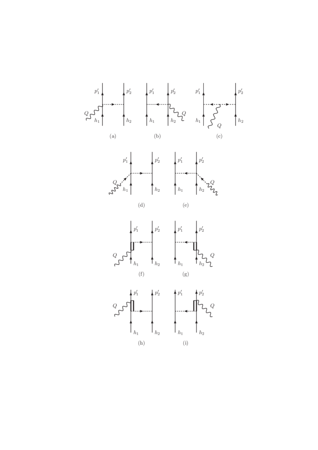
Figure 1: Feynman diagrams of the MEC considered in the present study, including the seagull (a,b), pion-in-flight (c), pion-pole (d,e), and $\Delta$ pole (f–i).

In this section we describe our model for relativistic weak meson-exchange currents. We work at tree level including only one-pion exchange. The relativistic electromagnetic MEC has been widely studied previously for intermediate-energy electron scattering and expressions have been given for instance in Dek94 ; DePace:2003spn ; Amaro:2010iu . To obtain the weak two-body current we need the relativistic axial contribution. To our knowledge this current has not been written explicitly in the literature, so this is one of the novelties of this work. We start from the weak pion production model of Hernandez:2007qq , based on the non-linear $\sigma$-model. We take the pion-production amplitudes from the nucleon given there, and we couple a second nucleon-line to the emitted pion. The resulting MEC operator is written as the sum of four contributions, denoted as seagull, pion-in-flight, pion-pole and Delta-pole

$$j^{\mu}_{\rm MEC}=j^{\mu}_{\rm sea}+j^{\mu}_{\rm\pi}+j^{\mu}_{\rm pole}+j^{\mu}_{\rm\Delta}.$$ (12)

The corresponding Feynman diagrams are given in Fig. 1.

In this work we do not include the so-called nucleon-pole contributions. These can be considered a part of the nucleon correlations that contributes to the nuclear spectral function and final-state interactions (FSI), and are not considered genuine meson-exchange currents. Besides, the corresponding diagrams produce divergences in the quasielastic region and some kind of regularization Alb84 ; Amaro:2010iu ; Alb91 or subtraction of self-energy diagrams Gil97 ; Nie11 are required. The effect of correlations is taken into account, at least partially, in the one-body cross section by using a spectral function for the nucleon in the medium Nie04 ; Ben08 or alternatively, with the super-scaling approach Amaro:2004bs ; Meg15 .

Each one of the four MEC operators can be decomposed as a sum of vector $(V)$ and axial-vector $(A)$ currents. The vector operators also contribute to electron scattering and are constrained by electromagnetic probes, while the axial ones only appear in weak processes like neutrino scattering.

III.1 Seagull current

The weak seagull current depicted in Fig. 1, diagrams (a) and (b), can be written as:

$$j^{\mu}_{\rm sea}=\left(I_{V}\right)_{\pm}J^{\mu}_{\rm sea},$$ (13)

where

$$\left(I_{V}\right)_{\pm}=(I_{V})_{x}\pm i(I_{V})_{y}$$ (14)

stands for the $\pm$-component of the two-body isovector operator

$$\mbox{\boldmath$I$}_{V}=i\left[\mbox{\boldmath$\tau$}(1)\times\mbox{\boldmath$\tau$}(2)\right]$$ (15)

and $J^{\mu}_{\rm sea}$ is the isospin-independent seagull current, given as the sum of $V$ and $A$ components

$$J^{\mu}_{\rm sea}=\left(J^{\mu}_{\rm sea}\right)_{V}+\left(J^{\mu}_{\rm sea}\right)_{A}.$$ (16)

They have been derived from the contact term (CT) of the pion neutrino-production amplitudes from Hernandez:2007qq , and can be written as

$$\left(J^{\mu}_{\rm sea}\right)_{V} = \frac{f^{2}_{\pi NN}}{m^{2}_{\pi}}F^{V}_{1}(Q^{2})V^{(s^{\prime}_{1},s_{1})}_{\pi NN}({\bf p}^{\prime}_{1},{\bf h}_{1})$$ (17)

$$\times \bar{u}_{s^{\prime}_{2}}({\bf p}^{\prime}_{2})\gamma_{5}\gamma^{\mu}u_{s_{2}}({\bf h}_{2})-(1\leftrightarrow 2)$$

$$\left(J^{\mu}_{sea}\right)_{A} = \frac{f^{2}_{\pi NN}}{m^{2}_{\pi}}\frac{1}{g_{A}}V^{(s^{\prime}_{1},s_{1})}_{\pi NN}({\bf p}^{\prime}_{1},{\bf h}_{1})F_{\rho}\left(k_{22}^{2}\right)$$ (18)

$$\times \bar{u}_{s^{\prime}_{2}}({\bf p}^{\prime}_{2})\,\gamma^{\mu}\,u_{s_{2}}({\bf h}_{2})-(1\leftrightarrow 2).$$

In these equations:

• The coupling constant $f_{\pi NN}/m_{\pi}$ comes from the $W^{\pm}\pi$NN and $\pi$NN vertices. In the $A$ component the Goldberger-Treiman relation has been applied to the amplitudes of Hernandez:2007qq

  $$\frac{g_{A}}{2f_{\pi}}=\frac{f_{\pi NN}}{m_{\pi}},$$ (19)

  with $g_{A}=1.26$ and $f_{\pi}=93$ MeV being, respectively, the nucleon axial coupling and the pion decay constant.

• The same form factors as in Hernandez:2007qq are used. $F^{V}_{1}(Q^{2})$ is the vector nucleon form factor, and $F_{\rho}(k^{2})$ accounts for the $\rho$-meson dominance of the $\pi\pi$NN coupling.

• The pion four-momenta $k_{ij}$ are the differences between the final and initial nucleon four-momenta in the $\pi$NN vertex, i.e.,

  $$k_{ij}=p^{\prime}_{i}-h_{j},\quad i,j=1,2.$$ (20)

• The function

  $$V^{(s^{\prime}_{i},s_{j})}_{\pi NN}({\bf p}^{\prime}_{i},{\bf h}_{j})=\frac{\bar{u}_{s^{\prime}_{i}}({\bf p}^{\prime}_{i})\,\gamma_{5}\not{\!k}_{ij}\,u_{s_{j}}({\bf h}_{j})}{k^{2}_{ij}-m^{2}_{\pi}}$$ (21)

  accounts for the propagation and subsequent absorption of the exchanged pion and includes the pion propagator and the $\pi NN$ vertex (see Fig. 1, diagrams (a),(b)). Note that for on-shell nucleons the following relation can be used to simplify the expression of $V_{\pi NN}$

  $$\bar{u}_{s^{\prime}_{i}}({\bf p}^{\prime}_{i})\gamma_{5}\not{\!k}_{ij}\,u_{s_{j}}({\bf h}_{j})=-2m\bar{u}_{s^{\prime}_{i}}({\bf p}^{\prime}_{i})\gamma_{5}u_{s_{j}}({\bf h}_{j}).$$ (22)

• The Cabibbo angle $\theta_{c}$, which was present in the amplitudes of Hernandez:2007qq , has been factorized out from the weak currents, and has been included in the definition of the factor $\sigma_{0}$ in Eq. (1).

• The shorthand notation $(1\leftrightarrow 2)$ means to interchange the ordering in the labels of the two nucleons’ spins and momenta, but not the isospins. Note that the $j^{\mu}_{\rm sea}$ current has to be understood as an operator in isospin space and a matrix element in spin-coordinate space. The symmetrization of the above operator is automatically taken into account due to the antisymmetry of the isovector isospin operator $\left(I_{V}\right)_{\pm}$ under the exchange of $(1\leftrightarrow 2).$

Finally, note that the electromagnetic current operator can be obtained from the above equations by keeping only the $V$ current and taking the $z$ component of the isospin operator

$$(I_{V})_{\pm}\rightarrow(I_{V})_{z}=i\left[\mbox{\boldmath$\tau$}(1)\times\mbox{\boldmath$\tau$}(2)\right]_{z}.$$ (23)

The resulting electromagnetic seagull current is in agreement with previous expressions VanOrden:1980tg ; DePace:2003spn ; Amaro:2010iu .

III.2 Pion-in-flight term

The weak pion-in-flight current, depicted in diagram (c) of Fig. 1, can be expressed in a similar way to the seagull operator, but with a vanishing axial part:

$$j^{\mu}_{\pi} = \left(I_{V}\right)_{\pm}\,J^{\mu}_{\pi}$$ (24)

$$J^{\mu}_{\pi} = \left(J^{\mu}_{\pi}\right)_{V}+\left(J^{\mu}_{\pi}\right)_{A}$$ (25)

$$\left(J^{\mu}_{\pi}\right)_{V} = \frac{f^{2}_{\pi NN}}{m^{2}_{\pi}}F^{V}_{1}(Q^{2})V^{(s^{\prime}_{1},s_{1})}_{\pi NN}({\bf p}^{\prime}_{1},{\bf h}_{1})$$ (26)

$$\times V^{(s^{\prime}_{2},s_{2})}_{\pi NN}({\bf p}^{\prime}_{2},{\bf h}_{2})\left(k^{\mu}_{11}-k^{\mu}_{22}\right)$$

$$\left(J^{\mu}_{\pi}\right)_{A} = 0.$$ (27)

Equation (26) reproduces the well-known expression for the pion-in-flight electromagnetic MEC taking the $z$ component of the isospin operator VanOrden:1980tg ; DePace:2003spn ; Amaro:2010iu . It corresponds to the so-called PF piece of the pion production amplitudes of Hernandez:2007qq .

III.3 Pion-pole term

At variance with the pion-in-flight current, the pion-pole term (diagrams (d) and (e) of Fig. 1) has only the axial component and therefore it is absent in the electromagnetic case. This new contribution could be considered as the “axial counterpart” of the pion-in-flight term, in the sense that it contains two pion propagators and is proportional to $k_{11}+k_{22}=Q$. The expression for this current is:

$$j^{\mu}_{\rm pole} = \left(I_{V}\right)_{\pm}J^{\mu}_{\rm pole}$$ (28)

$$J^{\mu}_{\rm pole} = \left(J^{\mu}_{\rm pole}\right)_{V}+\left(J^{\mu}_{\rm pole}\right)_{A}$$ (29)

$$\left(J^{\mu}_{\rm pole}\right)_{V} = 0$$ (30)

$$\left(J^{\mu}_{\rm pole}\right)_{A} = \frac{f^{2}_{\pi NN}}{m^{2}_{\pi}}\frac{1}{g_{A}}F_{\rho}\left(k_{11}^{2}\right)V^{(s^{\prime}_{2},s_{2})}_{\pi NN}({\bf p}^{\prime}_{2},{\bf h}_{2})$$ (31)

$$\times Q^{\mu}\;\frac{\bar{u}_{s^{\prime}_{1}}({\bf p}^{\prime}_{1})\not{\!Q}\;u_{s_{1}}({\bf h}_{1})}{Q^{2}-m^{2}_{\pi}}-(1\leftrightarrow 2).$$

Note the similarity with the axial part of the seagull current because it has the same form factor and it contains a factor $1/g_{A}$. Since it is proportional to $Q^{\mu}$, this current only contributes to the longitudinal and time components of the hadronic tensor.

III.4 $\Delta(1232)$ term

The $\Delta$-pole terms correspond in Fig. 1 to diagrams (f,g) for the forward and (h,i) for the backward $\Delta$ propagations, respectively. We start from the $\Delta$-pole and the crossed-$\Delta$-pole pion-production amplitudes of Hernandez:2007qq . Attaching a second nucleon which absorbs the pion, we obtain the following currents

$$j^{\mu}_{\Delta} =j^{\mu}_{\Delta,\rm forw}+j^{\mu}_{\Delta,\rm back}$$ (32)

$$j^{\mu}_{\Delta,\rm forw} =-\frac{f^{*}f_{\pi NN}}{m^{2}_{\pi}}\,\sqrt{3}\left(U^{\rm forw}\right)_{t^{\prime}_{1}t^{\prime}_{2};t_{1}t_{2}}\;V^{(s^{\prime}_{2},s_{2})}_{\pi NN}({\bf p}^{\prime}_{2},{\bf h}_{2})$$

$$\times k^{\alpha}_{22}\,\bar{u}_{s^{\prime}_{1}}({\bf p}^{\prime}_{1})G_{\alpha\beta}(h_{1}+Q)\Gamma^{\beta\mu}(h_{1},Q)u_{s_{1}}({\bf h}_{1})$$

$$+(1\leftrightarrow 2)$$ (33)

$$j^{\mu}_{\Delta,\rm back} =-\frac{f^{*}f_{\pi NN}}{m^{2}_{\pi}}\,\sqrt{3}\left(U^{\rm back}\right)_{t^{\prime}_{1}t^{\prime}_{2};t_{1}t_{2}}\;V^{(s^{\prime}_{2},s_{2})}_{\pi NN}({\bf p}^{\prime}_{2},{\bf h}_{2})$$

$$\times k^{\beta}_{22}\,\bar{u}_{s^{\prime}_{1}}({\bf p}^{\prime}_{1})\hat{\Gamma}^{\mu\alpha}(p^{\prime}_{1},Q)G_{\alpha\beta}(p^{\prime}_{1}-Q)u_{s_{1}}({\bf h}_{1})$$

$$+(1\leftrightarrow 2).$$ (34)

The meaning of the different quantities in these equations is as follows:

• The $\pi N\Delta$ coupling constant is denoted $f^{*}=2.13$.

• The $\Delta$-propagator $G_{\alpha\beta}(P)$ is described by the Rarita-Schwinger propagator of a spin 3/2 particle

  $$G_{\alpha\beta}(P)=\frac{P_{\alpha\beta}(P)}{P^{2}-M^{2}_{\Delta}+iM_{\Delta}\Gamma_{\Delta}(P^{2})},$$ (35)

  where $P_{\alpha\beta}$ is the projector over spin-$\frac{3}{2}$ ,

  $$P_{\alpha\beta}(P) =-(\not{\!P}+M_{\Delta})\left[g_{\alpha\beta}-\frac{1}{3}\gamma_{\alpha}\gamma_{\beta}-\frac{2}{3}\frac{P_{\alpha}P_{\beta}}{M^{2}_{\Delta}}\right.$$

  $$+\left.\frac{1}{3}\frac{P_{\alpha}\gamma_{\beta}-P_{\beta}\gamma_{\alpha}}{M_{\Delta}}\right]$$ (36)

  and $M_{\Delta}$ and $\Gamma_{\Delta}$ stand for the $\Delta(1232)$ resonance mass and width, respectively.

• In the forward piece, we have introduced the weak $N\rightarrow\Delta$ transition vertex written as the sum of vector and axial-vector vertices

  $$\Gamma^{\beta\mu}(P,Q) =\Gamma^{\beta\mu}_{V}(P,Q)+\Gamma^{\beta\mu}_{A}(P,Q)$$ (37)

  $$\Gamma^{\beta\mu}_{V}(P,Q) =\left[\frac{C^{V}_{3}}{M}\left(g^{\beta\mu}\not{\!Q}-Q^{\beta}\gamma^{\mu}\right)\right.$$

  $$+\left.\frac{C^{V}_{4}}{M^{2}}\left(g^{\beta\mu}Q\cdot P_{\Delta}-Q^{\beta}P^{\mu}_{\Delta}\right)\right.$$ (38)

  $$+\left.\frac{C^{V}_{5}}{M^{2}}\left(g^{\beta\mu}Q\cdot P-Q^{\beta}P^{\mu}\right)+C^{V}_{6}g^{\beta\mu}\right]\gamma_{5}$$

  $$\Gamma^{\beta\mu}_{A}(P,Q) =\frac{C^{A}_{3}}{M}\left(g^{\beta\mu}\not{\!Q}-Q^{\beta}\gamma^{\mu}\right)$$

  $$+\frac{C^{A}_{4}}{M^{2}}\left(g^{\beta\mu}Q\cdot P_{\Delta}-Q^{\beta}P^{\mu}_{\Delta}\right)$$

  $$+C^{A}_{5}g^{\beta\mu}+\frac{C^{A}_{6}}{M^{2}}Q^{\beta}Q^{\mu},$$ (39)

  with $P_{\Delta}=P+Q$.

  The symbols $C^{V,A}_{i}$ ($i=3-6$) in the above equations stand for the $Q^{2}$-dependent vector and axial-vector form factors.

• In the backward term we use instead the $\Delta\rightarrow N$ transition vertex given by

  $$\hat{\Gamma}^{\mu\alpha}(P^{\prime},Q)=\gamma^{0}\left[\Gamma^{\alpha\mu}(P^{\prime},-Q)\right]^{\dagger}\gamma^{0}.$$ (40)

• The quantities $(U^{\rm forw})_{t^{\prime}_{1}t^{\prime}_{2};t_{1}t_{2}}$ and $(U^{\rm back})_{t^{\prime}_{1}t^{\prime}_{2};t_{1}t_{2}}$ are the matrix elements of the following forward and backward isospin operators

  $$U^{\rm forw} = \left(T_{i}\left(T^{\dagger}\right)_{+1}\right)\otimes\tau_{i}$$ (41)

  $$U^{\rm back} = \left(T_{+1}\,T^{\dagger}_{i}\right)\otimes\tau_{i},$$ (42)

  where $T_{+1}$ is the spherical component of the isovector transition operator $\frac{3}{2}\rightarrow\frac{1}{2}$, normalized as

  $$\left\langle\frac{3}{2},t_{\Delta}\Big{|}(T^{\dagger})_{\lambda}\Big{|}\frac{1}{2},t_{N}\right\rangle=C\left(\frac{1}{2},1,\frac{3}{2}\Big{|}t_{N},\lambda,t_{\Delta}\right)$$ (43)

  for $\lambda=\pm 1,0$.

III.5 Isospin structure of MEC

The isospin dependence of the $\Delta$ current is more complex than the other operators (seagull, pion-in-flight, and pion-pole). However, it is possible to expand the $U^{\rm forw,back}$ operators as linear combinations of the three basic isospin matrices $\mbox{\boldmath$\tau$}(1),\mbox{\boldmath$\tau$}(2)$, and $\mbox{\boldmath$I$}_{V}$. This is a consequence of the following basic property of the isospin transition operators in cartesian coordinates:

$$T_{i}\,T^{\dagger}_{j}=\frac{2}{3}\,\delta_{ij}-\frac{i}{3}\,\epsilon_{ijk}\,\tau_{k}.$$ (44)

From this relation it follows that

$$\sqrt{3}\,U^{\rm forw} =\frac{1}{\sqrt{6}}\left[-2\,\tau_{{}_{+}}(2)+\left(I_{V}\right)_{+}\right]$$ (45)

$$\sqrt{3}\,U^{\rm back} =\frac{1}{\sqrt{6}}\left[-2\,\tau_{{}_{+}}(2)-\left(I_{V}\right)_{+}\right]$$ (46)

Analogously, in the $(1\leftrightarrow 2)$ terms of Eqs. (33,34) the isospin operators have to be modified by making the change

$$\sqrt{3}\,U^{\rm forw} \quad\underrightarrow{{}^{(1\leftrightarrow 2)}}\quad\frac{1}{\sqrt{6}}\left[-2\,\tau_{{}_{+}}(1)-\left(I_{V}\right)_{+}\right]$$ (47)

$$\sqrt{3}\,U^{\rm back} \quad\underrightarrow{{}^{(1\leftrightarrow 2)}}\quad\frac{1}{\sqrt{6}}\left[-2\,\tau_{{}_{+}}(1)+\left(I_{V}\right)_{+}\right],$$ (48)

where we have made use of the antisymmetry property of the isovector operator $\mbox{\boldmath$I$}_{V}=i\left(\mbox{\boldmath$\tau$}(1)\times\mbox{\boldmath$\tau$}(2)\right)$ under the interchange $(1\leftrightarrow 2)$.

Substituting these relations in Eqs. (33,34), it is clear that the $\Delta$-current operator can be written as the sum of three currents, each one characterized by a specific isospin dependence

$$j^{\mu}_{\Delta} =\tau_{+}(1)\;J^{\mu}_{\Delta 1}(1^{\prime},2^{\prime};\,1,2)+\tau_{+}(2)\;J^{\mu}_{\Delta 2}(1^{\prime},2^{\prime};\,1,2)$$

$$+\left(I_{V}\right)_{+}\;J^{\mu}_{\Delta 3}(1^{\prime},2^{\prime};\,1,2),$$ (49)

where the three functions $J^{\mu}_{\Delta i}(1^{\prime},2^{\prime};\,1,2)$ depend only on spins and momenta.

This expression for neutrinos can be applied to antineutrinos by taking the $(-)$ component of the isospin operators. In the same way, for electron scattering one should take the $z$ component of the isospin operators and keep only the $V$ part of the current. The resulting electromagnetic $\Delta$ current is in agreement with previous expressions Amaro:2010iu .

From Eqs. (13, 24, 28, 49) we note that the total CC MEC for neutrino scattering can be written as

$$j^{\mu}_{\rm MEC} = \tau_{+}(1)\,J^{\mu}_{1}(1^{\prime}\,2^{\prime};1\,2)+\tau_{+}(2)\,J^{\mu}_{2}(1^{\prime}\,2^{\prime};1\,2)$$ (50)

$$+ \left(I_{V}\right)_{+}\,J^{\mu}_{3}(1^{\prime}\,2^{\prime};1\,2),$$

where

$$J_{1}^{\mu} = J_{\Delta 1}^{\mu}$$ (51)

$$J^{\mu}_{2} = J^{\mu}_{\Delta 2}$$ (52)

$$J^{\mu}_{3} = J^{\mu}_{\rm sea}+J^{\mu}_{\pi}+J^{\mu}_{\rm pole}+J^{\mu}_{\Delta 3}.$$ (53)

This explicitly shows that the CC MEC operators transform as irreducible vectors in isospin space, implying in particular that the final 2p-2h nuclear states must have $T=1$ for isoscalar nuclei ($T=0$). Expression (50) will be useful in obtaining the response functions for the separate charge channels because the action of the three operators $\tau_{+}(1)$, $\tau_{+}(2)$, and $(I_{V})_{+}$ can be computed directly (see Appendix A).

IV Electroweak response functions

In the previous section we presented the expressions for the currents in our fully relativistic model of MEC. These currents were derived from the pion production amplitudes of Hernandez:2007qq . In this section we give the explicit expressions for the weak response functions in the different 2p-2h charge channels.

IV.1 $(\nu_{l},l^{-})$ responses

CC neutrino scattering can induce two possible 2p-2h transitions: $np\rightarrow pp$ and $nn\rightarrow np$. In the first case, the $pp$ emission channel, the diagonal components of the hadronic tensor are of the type

$$W^{\mu\mu}_{pp} = \frac{1}{2}\sum\kern-15.0694pt\int\kern 4.30554pt\left|\langle pp|j^{\mu}_{MEC}(1^{\prime}2^{\prime};12)\right.$$ (54)

$$\left.-j^{\mu}_{MEC}(2^{\prime}1^{\prime};12)|np\rangle\right|^{2},$$

where for brevity we have defined a symbol implying an integration over momenta and a sum over nucleon spins

$$\sum\kern-15.0694pt\int\kern 4.30554ptf(1^{\prime}2^{\prime};12) \equiv \frac{V}{(2\pi)^{9}}\int d^{3}p^{\prime}_{1}d^{3}h_{1}d^{3}h_{2}\frac{M^{4}}{E_{1}E_{2}E^{\prime}_{1}E^{\prime}_{2}}$$ (55)

$$\Theta(p^{\prime}_{1},p^{\prime}_{2},h_{1},h_{2})\sum_{s_{1}s_{2}s^{\prime}_{1}s^{\prime}_{2}}f(1^{\prime}2^{\prime};12)$$

$$\delta(E^{\prime}_{1}+E^{\prime}_{2}-E_{1}-E_{2}-\omega),$$

where $f(1^{\prime}2^{\prime};12)$ is any function depending on the momenta and spins of the final 2p-2h states.

Note that in the second line of Eq. (54) we have exchanged the momenta and spins of the final protons. Here we do not apply the general Eq. (LABEL:elementary) which provides the total elementary hadronic tensor including all the charge channels.

Using the expansion in Eq. (50) we get

$$W^{\mu\mu}_{pp} = \frac{1}{2}\sum\kern-15.0694pt\int\kern 4.30554pt\left|\langle pp|\tau^{(1)}_{+}J^{\mu}_{1}(1^{\prime}2^{\prime};12)+\tau^{(2)}_{+}J^{\mu}_{2}(1^{\prime}2^{\prime};12)\right.$$ (56)

$$\left.+(I_{V})_{+}J^{\mu}_{3}(1^{\prime}2^{\prime};12)\right.$$

$$\left.-\tau^{(1)}_{+}J^{\mu}_{1}(2^{\prime}1^{\prime};12)-\tau^{(2)}_{+}J^{\mu}_{2}(2^{\prime}1^{\prime};12)\right.$$

$$-(I_{V})_{+}J^{\mu}_{3}(2^{\prime}1^{\prime};12)|np\rangle\Big{|}^{2}.$$

The isospin matrix elements can be computed from Eqs. (72–74) of Appendix A, resulting in

$$W^{\mu\mu}_{pp} = 2\sum\kern-15.0694pt\int\kern 4.30554pt\left|J^{\mu}_{1}(1^{\prime}2^{\prime};12)+J^{\mu}_{3}(1^{\prime}2^{\prime};12)\right.$$ (57)

$$\left.-J^{\mu}_{1}(2^{\prime}1^{\prime};12)-J^{\mu}_{3}(2^{\prime}1^{\prime};12)\right|^{2}.$$

Notice that this is written as the square of direct minus exchange matrix elements of the following “effective current” for $pp$-emission with neutrinos

$$J_{pp}^{\mu}=J_{1}^{\mu}+J_{3}^{\mu}.$$ (58)

Changing variables $1^{\prime}\leftrightarrow 2^{\prime}$ in the final state, it can be demonstrated that the contribution of the square of the exchange and direct parts are equal. Thus we obtain

$$W^{\mu\mu}_{pp} = 4\sum\kern-15.0694pt\int\kern 4.30554pt\left\{\left|J^{\mu}_{pp}(1^{\prime}2^{\prime};12)\right|^{2}\right.$$ (59)

$$-{\rm Re}\;J^{\mu}_{pp}(1^{\prime}2^{\prime};12)^{*}J^{\mu}_{pp}(2^{\prime}1^{\prime};12)\Big{\}}.$$

The first term is usually called the “direct” contribution, and the second one is the “exchange” contribution, actually being the interference between the direct and exchange matrix elements. The exchange contributions to the 2p-2h cross section have not been included in the existing models of neutrino scattering Nie11 ; Mar09 , whereas in this work we include them. In Fig. 2 we show a many-body diagrammatic representation of the direct and exchange contributions.

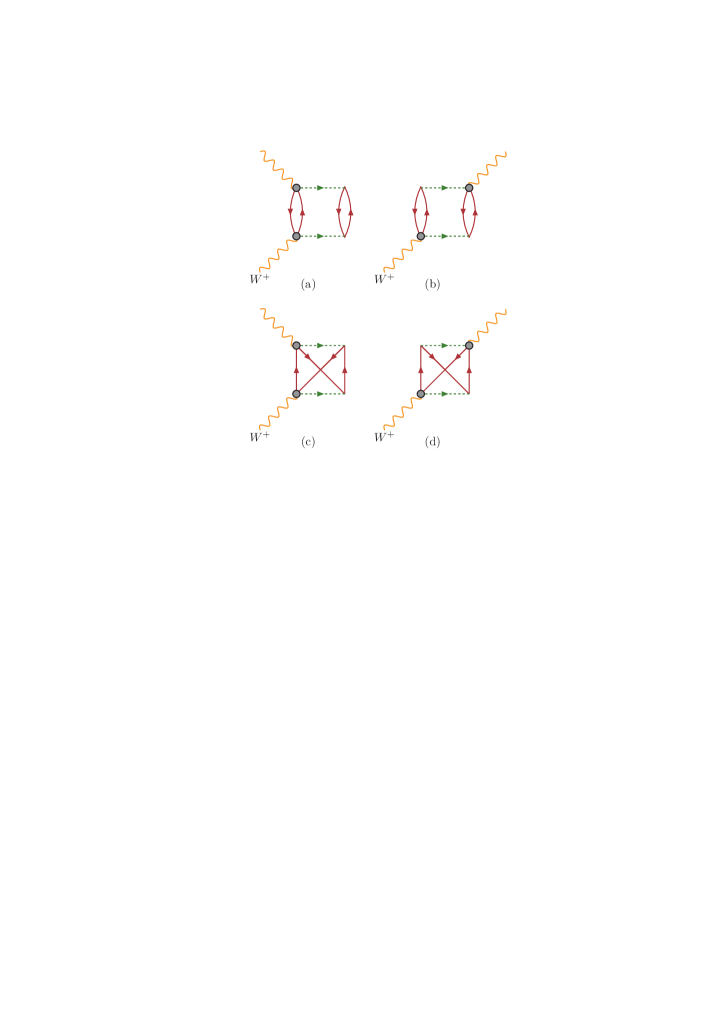
Figure 2: Some contributions of 2p-2h to the virtual $W^{+}$ self-energy, or polarization propagator $\Pi^{\mu\nu}$. The response functions considered in this work are related to the imaginary part of the polarization propagator, ${\rm Im}\;\Pi^{\mu\nu}$. The circle stands for the elementary model for $W^{+}N\rightarrow\pi N$ of Hernandez:2007qq without the nucleon-pole diagrams. Diagrams (a,b) represent the direct contribution. Diagrams (c,d) are the exchange contributions.

The $np$ emission case can be obtained in a similar way, the only difference being that now the exchanged particles should be the two initial neutrons. We obtain

$$W^{\mu\mu}_{np} = 4\sum\kern-15.0694pt\int\kern 4.30554pt\left\{\left|J^{\mu}_{np}(1^{\prime}2^{\prime};12)\right|^{2}\right.$$ (60)

$$-{\rm Re}\;J^{\mu}_{np}(1^{\prime}2^{\prime};12)^{*}J^{\mu}_{np}(1^{\prime}2^{\prime};21)\Big{\}},$$

where the effective current for $np$ emission with neutrinos has been defined

$$J^{\mu}_{np}=J^{\mu}_{2}+J^{\mu}_{3}.$$ (61)

final state	$\nu$	$\overline{\nu}$	$e$
$pp$	$J_{1}+J_{3}$	$\times$	$J_{1}+J_{2}$
$np$	$J_{2}+J_{3}$	$J_{1}-J_{3}$	$-J_{1}+J_{2}$
			$2J_{3}$
$nn$	$\times$	$J_{2}-J_{3}$	$-J_{1}-J_{2}$

Table 1: Effective currents for two-nucleon emission that appear in the different charge channels for (anti) neutrinos and electrons (see text).

The above equations allow one to compute the diagonal hadronic tensor components appearing in the $LL,CC$ and $T$ responses. To compute the $CL$ and $T^{\prime}$ responses the non-diagonal hadronic tensor components are necessary. They are computed in a similar way, resulting in

$$W^{\mu\nu}_{pp} = 4\sum\kern-15.0694pt\int\kern 4.30554pt\Big{\{}J^{\mu}_{pp}(1^{\prime}2^{\prime};12)^{*}J^{\nu}_{pp}(1^{\prime}2^{\prime};12)$$ (62)

$$-J^{\mu}_{pp}(1^{\prime}2^{\prime};12)^{*}J^{\nu}_{pp}(2^{\prime}1^{\prime};12)\Big{\}}$$

$$W^{\mu\nu}_{np} = 4\sum\kern-15.0694pt\int\kern 4.30554pt\Big{\{}J^{\mu}_{np}(1^{\prime}2^{\prime};12)^{*}J^{\nu}_{np}(1^{\prime}2^{\prime};12)$$ (63)

$$-J^{\mu}_{np}(1^{\prime}2^{\prime};12)^{*}J^{\nu}_{np}(1^{\prime}2^{\prime};21)\Big{\}}.$$

IV.2 $(\bar{\nu}_{l},l^{+})$ responses

In the case of antineutrinos the allowed charge 2p-2h channels are $np\rightarrow nn$ and $pp\rightarrow np$. The corresponding formulae are obtained following the lines of the previous section, by taking the matrix elements of the $(-)$ isospin components of the MEC. The results are similar to Eqs. (59,60,62,63), by using the effective currents given in Table 1.

IV.3 $(e,e^{\prime})$ responses

In the case of electron scattering the three charge channels are all active. We take the matrix elements of the $z$-component of the MEC in isospin space. In the $pp$ and $nn$ cases the effective currents are given also in Table 1. For $np$ emission with electrons two effective currents appear, namely

$$W^{\mu\mu}_{pp} = \frac{1}{2}\sum\kern-15.0694pt\int\kern 4.30554pt\left\{\left|J^{\mu}_{pp}(1^{\prime}2^{\prime};12)\right|^{2}\right.$$ (64)

$$-{\rm Re}\;J^{\mu}_{pp}(1^{\prime}2^{\prime};12)^{*}J^{\mu}_{pp}(1^{\prime}2^{\prime};21)\Big{\}}$$

$$W^{\mu\mu}_{nn} = W^{\mu\mu}_{pp}$$ (65)

$$W^{\mu\mu}_{np} = \sum\kern-15.0694pt\int\kern 4.30554pt\left\{\left|J^{\mu}_{np1}(1^{\prime}2^{\prime};12)\right|^{2}+\left|J^{\mu}_{np2}(1^{\prime}2^{\prime};12)\right|^{2}\right.$$ (66)

$$+2{\rm Re}\;J^{\mu}_{np1}(1^{\prime}2^{\prime};12)^{*}J^{\mu}_{np2}(2^{\prime}1^{\prime};12)\Big{\}},$$

where the two effective currents are

$$J^{\mu}_{np1} = -J^{\mu}_{1}+J^{\mu}_{2}$$ (67)

$$J^{\mu}_{np2} = 2J^{\mu}_{3}.$$ (68)

These are summarized in fourth column of Table I.

V Treatment of the $\Delta$ current

In this section we provide the details of the treatment of the $\Delta$ current in our model and compare with other approaches.

The relativistic $\Delta$ current contribution to the electromagnetic $R^{T}$ response was first computed in Dek94 and DePace:2003spn . These authors started with the Peccei lagrangian for the $\gamma N\Delta$ interaction Pec69 . This introduces a difference with respect to the vector interaction given in Eq. (38). The Peccei vertex only includes the $O(1/M)$ term that should correspond to the $C_{3}^{V}/M$ term of Eq. (38). There is still another difference between the two approaches because the Peccei vertex includes a contraction with the tensor

$$\Theta^{\mu\nu}=g^{\mu\nu}-\frac{1}{4}\gamma^{\mu}\gamma^{\nu}.$$ (69)

This tensor takes into account possible off-shellness effects of the virtual $\Delta$ Pas95 . In the case the $\Delta$ is on-shell, this is reduced to $g^{\mu\nu}$ because of the properties of Rarita-Schwinger spinors.

We have verified that upon multiplying the above tensor by the first term of Eq. (38) the $\Delta$ current of DePace:2003spn is reproduced. This is a consequence of the identity

$$\Theta^{\beta\nu}(g_{\nu}^{\mu}\not{\!Q}-Q_{\nu}\gamma^{\mu})=\frac{1}{2}(Q^{\mu}\gamma^{\beta}-\gamma^{\mu}\not{\!Q}\gamma^{\beta}).$$ (70)

The resulting current coincides with the one given in DePace:2003spn (notice that there is a relative minus sign with respect to Eq. (35) in the definition of the $\Delta$ propagator in that reference). We have checked numerically that the inclusion of $\Theta^{\mu\nu}$ has a negligible effect on the transverse response at the kinematics relevant for this work, and therefore it will not be included in the calculations.

Therefore in this work we are using exactly the same operator as in DePace:2003spn for the $\Delta$ vector current, corresponding to the term $C_{3}^{V}/M$ in Eq. (38). We neglect the terms $C_{4}^{V}$ and $C_{5}^{V}$ ($C_{6}^{V}=0$ by conservation of vector current) that are expected to give much smaller contributions because they are supressed by $O(P/M)$. To be consistent, in the axial part we only include the leading contribution of Eq. (39), proportional to $C_{5}^{A}$ and neglect the other terms.

In what follows we discuss the important point concerning the ambiguity related to the theoretical separation between 2p-2h and $\Delta$-peak contributions. The $\Delta$ peak is the main contribution to the pion production cross section. But inside the nucleus the $\Delta$ can also decay into one nucleon that re-scatters producing two-nucleon emission without pions. Therefore this decay of the $\Delta$ should be considered part of the 2p-2h channel. Let us consider the diagram of Fig. 3. This diagram is implicitly included in our calculation, being one of the contributions to diagram (a) of Fig. 2. Thus, it can be considered to contribute to the 2p-2h responses and/or to the $\Delta$ peak. In fact this diagram contains one self-energy insertion contributing to dressing the $\Delta$ propagator. As a consequence, there is no unique way of separating the $\Delta$ emission from the 2p-2h channels because $\Delta$ emission already includes 2p-2h decays inside the nucleus.

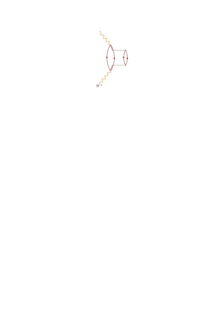
Figure 3: Direct term of the MEC with excitation of an intermediate $\Delta$ decaying into a 2p-1h state.

Hence, the MEC contribution given by Eq. (9), while being purely 2p-2h, also contributes to some extent to the $\Delta$ peak and, conversely, any calculation of the $\Delta$ peak including a dressed $\Delta$ propagator would include implicitly some contribution from the diagram of Fig. 3. It is a matter of choice in building some specific model whether this contribution is regarded as part of the 2p-2h or $\Delta$ peak responses. Here we include it in the 2p-2h response.

The previous discussion should make clear that a comparison between models of MEC that use different prescriptions for the treatment of the $\Delta$-pole makes no sense, as long as they contain different admixtures of $\Delta$ emission. In other words, it is only the total cross section that is meaningful and worthwhile to compare.

Before providing reliable predictions for neutrino scattering, any model must be validated by confronting it with quasielastic electron scattering data. Thus the validation of any prescription for the MEC contribution requires one to compute the total $(e,e^{\prime})$ cross section with a model that includes also both the quasielastic and inelastic contributions. The validation of our prescription for electron scattering has been recently performed in Meg16 , where we have shown that the experimental world-data for ¹²C can be nicely reproduced within the super-scaling approach SuSAv2 using the MEC of DePace:2003spn . For other models this necessary test has yet to be performed systematically.

VI Results

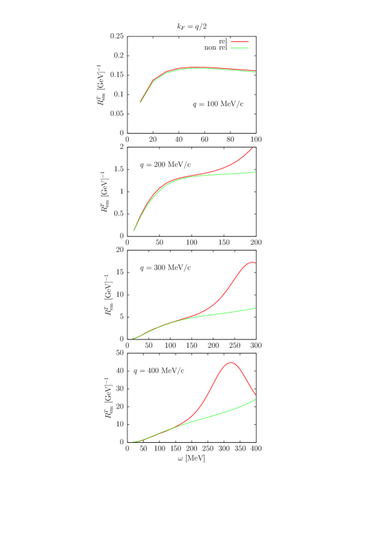
Figure 4: Electromagnetic transverse response function for 2p-2h for low momentum $q$ and $k_{F}=q/2$. Here we take $A=56$.

In this section we present results for the five 2p-2h response functions of neutrino scattering, as a function of $(q,\omega)$. This assumes that the energy of the incident neutrino is known. We study the dependence of the results on several ingredients of the model.

First we validate the relativistic currents for low energy and momentum transfer by comparison with the electromagnetic transverse response function computed in the non-relativistic limit. The relativistic and non-relativistic responses should coincide in this limit.

We follow the semi-analytical method of VanOrden:1980tg (see also Alb84 ; DePace:2003spn ) to compute the non-relativistic 2p-2h transverse response function in electron scattering. The comparison with the relativistic calculation also allows one to evaluate the size of the relativistic corrections. The non-relativistic model is described in Appendix B.

In Fig. 4 we show the electromagnetic $T$ response for low momentum transfer from $q=100$ to 400 MeV/c and mass number $A=56$. The value of the Fermi momentum is chosen to be $k_{F}=q/2$. This is so because the non-relativistic limit requires that all of the initial and final momenta go simultaneously to zero, and $k_{F}$ should also be reduced accordingly. Another reason to reduce $k_{F}$ in this non-relativistic test is that for $q<2k_{F}$ Pauli blocking may reduce considerably the response function and the comparison cannot be made.

In the figure we see that for $q=100$ MeV/c the relativistic and non-relativistic results are the same, and they start to differ only around $q=200$ MeV/c. The difference is due mainly to the $\Delta$ propagator, that in one case is considered constant, and in the other case has the relativistic energy-momentum dependence. In fact, for these low values of $q$, the maximum of the relativistic response appears around $\omega\sim M_{\Delta}-M\simeq 300$ MeV, which is the minimum energy needed to produce the $\Delta$ excitation for a nucleon at rest.

The case $q=400$ MeV/c and above, where $k_{F}$ takes realistic values, is characteristic of what one would expect when one uses a constant instead of the dynamical $\Delta$ propagator in the traditional non-relativistic calculations. Further insight can be seen in Fig. 5. The relativistic result with a constant $\Delta$ propagator is similar to the non-relativistic calculation. In this sense the relativistic effects coming from kinematics and spinors are smaller than the effects due to the dynamical $\Delta$ propagator.

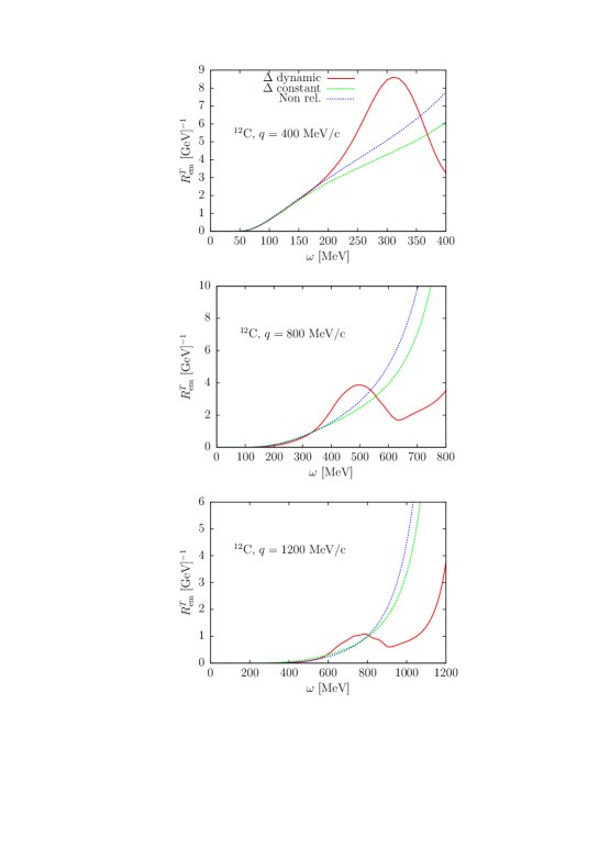
Figure 5: Electromagnetic 2p-2h transverse response function of ¹²C from low to high momentum $q$ and $k_{F}=228$ MeV/c. We show the total relativistic and non-relativistic results, compared to the relativistic result with a constant $\Delta$ propagator.

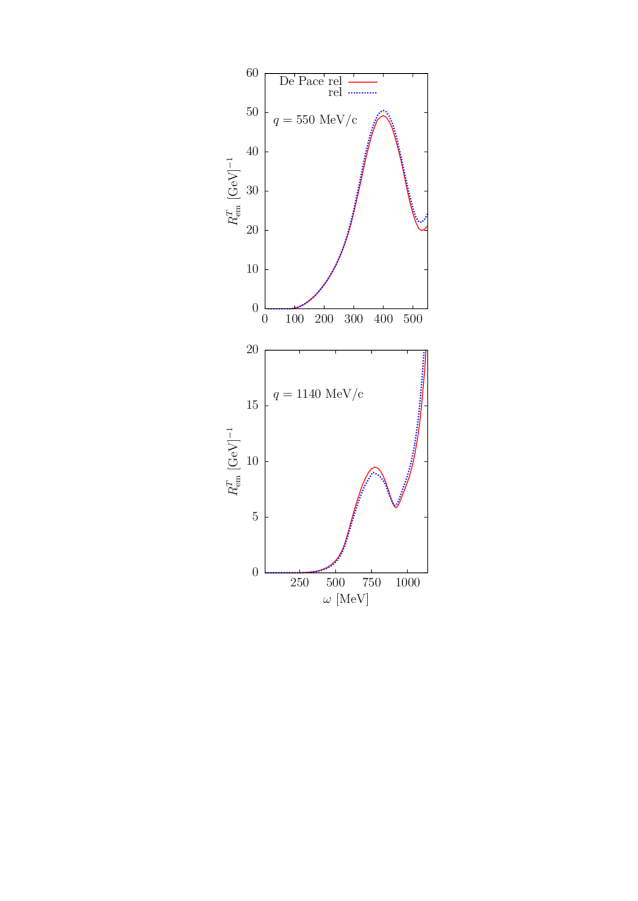
Figure 6: Electromagnetic transverse response function for 2p-2h from ⁵⁶Fe for two values of $q$. Comparison is made with the model of DePace:2003spn .

In Fig. 6 we compare our results with the calculation of De Pace et al. DePace:2003spn for ⁵⁶Fe ($k_{F}=260$ MeV/c), including the total MEC current with direct and exchange contributions. We use here the same ingredients as in DePace:2003spn for the electromagnetic and strong form factors, and also for the $\Delta$ width. Only the real part of the $\Delta$ propagator is included in this calculation, Eq. (35). The two models basically coincide, with only small differences attributed to the different numerical integration methods used. In this sense our model can be considered as an extension of the model of DePace:2003spn to the charge-changing weak sector.

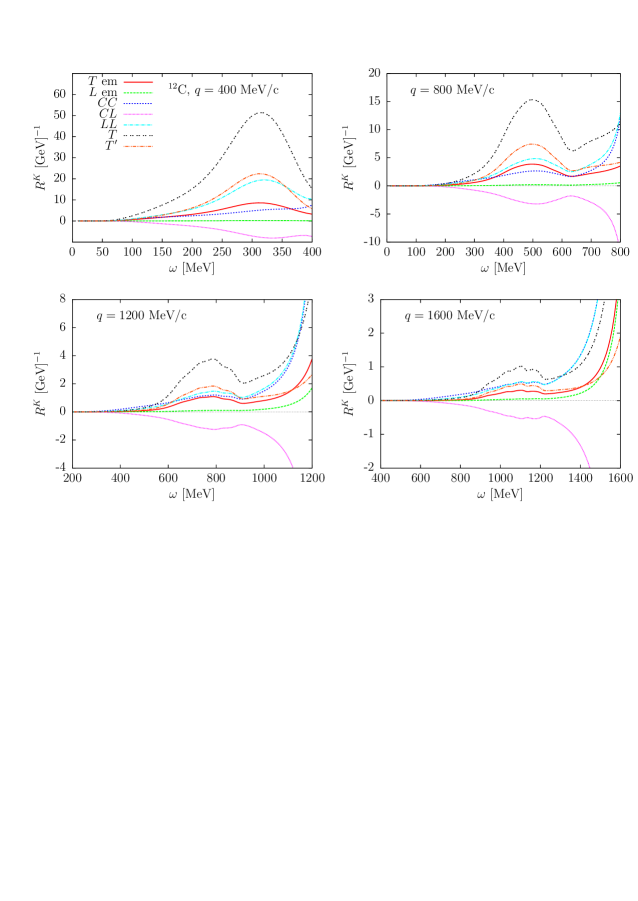
Figure 7: Separate 2p-2h response functions of ¹²C for four values of the momentum transfer. We show the $L$, $T$ electromagnetic responses and the five weak responses for charge-changing neutrino scattering. To distinguish results for charge-changing neutrino reactions from those for electron scattering we employ the subscript “em” for the latter and no subscript for the former.

In Fig. 7 we compare the separate 2p-2h response functions of ¹²C for four values of the momentum transfer. We use $k_{F}=228$ MeV/c and a separation energy $\epsilon=40$ MeV for the 2p-2h state. We show the $L$, $T$ electromagnetic responses and the five weak responses for CC neutrino scattering. The transverse response is dominant because it contains the additive contributions from the $V$ and $A$ currents. The electromagnetic longitudinal is negligible, but this is not the case for the neutrino CC response, indicating a large axial MEC contribution.

Here a few words are in order concerning the conventions being used. For electron scattering the transverse em response has two contributions, one isoscalar and one isovector. For the latter one typically uses matrix elements of an irreducible tensor operator in isospin space, for instance, for the one-body current, matrix elements of $\tau_{3}=\tau_{0}$, where $\tau_{m}$ with $m=0,\pm 1$ are the components of the irreducible tensor. On the other hand, for charge-changing weak processes it is conventional to use the raising and lowering operators, which for one-body currents go as $\tau_{\pm}=\mp\sqrt{2}\tau_{\pm 1}$, giving rise to a factor of 2 between the em isovector transverse response and the CC neutrino transverse $VV$ response, the latter being twice as large as the former with these conventions. Of course the em case also has isoscalar contributions, although these are typically quite small at high energies where the magnetization current dominates over the convection current, since the isoscalar to isovector ratio is roughly $\mu_{V}^{2}/\mu_{S}^{2}\simeq 30$. These arguments are more general and one finds the same factor for the two-body MEC. In fact, from Eqs. (59,60) and (64,65,66), by summing over all the isospin channels, the $VV$ $T$-response is proven to be twice the em $T$-response.

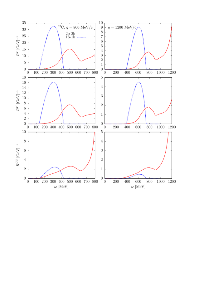
Figure 8: Comparison between 1p-1h and 2p-2h response functions for CC neutrino scattering off ¹²C for two values of the momentum transfer.

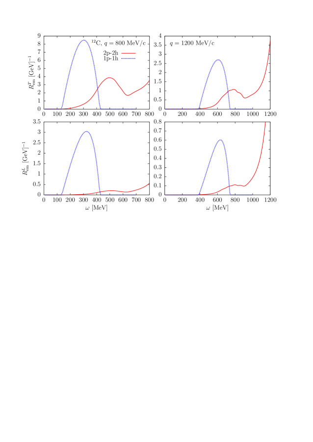
Figure 9: Comparison between 1p-1h and 2p-2h response functions for electron scattering off ¹²C for two values of the momentum transfer.

In Fig. 8 we compare the 1p-1h and 2p-2h neutrino responses for $q=800$ and 1200 MeV/c. The 1p-1h responses are computed in the RFG and only contain the one-body (OB) current. For these values of $q$ there are large MEC effects. The 2p-2h strength at the maximum of the $\Delta$ peak is around $50\%$ of the 1p-1h response. The MEC effects are similar in the $T$ and $T^{\prime}$ responses. The MEC effects in the $CC$ response are relatively much larger than in the transverse ones. This indicates again a large longitudinal contribution of the axial MEC.

It should be kept in mind, however, that each response function appears in the cross section multiplied by a kinematical factor (see Eq. (2)) which alters the balance shown in Fig. 7. For example, the contributions of the three responses $R^{CC}$, $R^{CL}$ and $R^{LL}$ largely cancel each other, yielding a net charge/longitudinal cross section that is generally smaller than the transverse ones. This balance of the different response functions of course depends on the kinematics.

For comparison, in Fig. 9 we show the electromagnetic response functions. Here the MEC effects in the transverse case are similar to those shown for neutrinos, while the longitudinal MEC contribution is very small except as one approaches the lightcone $(Q^{2}=0)$ where they become large. One should remember, however, that the kinematic factor $v_{L}$ that multiplies the longitudinal response goes to zero in the real-photon limit.

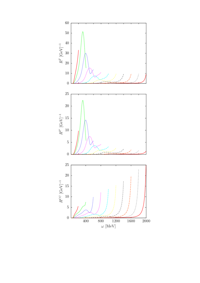
Figure 10: Evolution of the weak 2p-2h response functions from low to high values of $q$. Only the $T$, $T^{\prime}$ and $CC$ responses are shown from left to right, for $q=200$, 400, 600, 800, 1000, 1200, 1400, 1600, 1800 and 2000 MeV/c.

In Fig. 10 we show the behavior of three of the weak response functions from low to high $q$. The MEC peak moves from left to right according approximately to the $\Delta$ position $\omega\sim\sqrt{M_{\Delta}^{2}+q^{2}}-M$, and its strength decreases due to the form factors, since $Q^{2}$ at the peak position increases with $q$. While one might be tempted to conclude that the MEC contributions become negligible at high $q$, it should be remembered that the QE response also decreases as $q$ increases. In fact, a better representation of the relative importance of these two contributions can be obtained by forming the so-called reduced response used in scaling analyses, i.e., by dividing the responses by the single-nucleon expression that makes the QE response scale (see Donnelly:1998xg ; Meg15 ). In this representation the QE contribution plotted versus the corresponding scaling variable becomes universal — a single curve is obtained. Doing the same for the MEC contribution yields a better understanding of the relative importance of the two contributions. In fact, in going from low $q$ to 2000 MeV/c the MEC reduced response falls only by about a factor of two (see also Meg15 ). The $T$ and $T^{\prime}$ responses are similar in shape and the size of $R^{T}$ is around twice that of $R^{T^{\prime}}$.

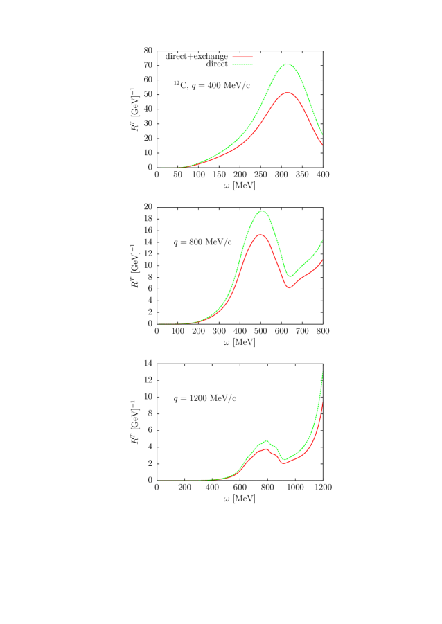
Figure 11: The $T$ weak response function computed including only the direct contribution compared to the direct+exchange contribution.

In Fig. 11 we show the effect of neglecting the exchange contribution (see diagrams (c), (d) of Fig. 2). This amounts to about a 25% increase. This is in agreement with DePace:2003spn and also with previous studies of the exchange pieces in the $\Delta$ self-energy Ose87 . We conclude, as in DePace:2003spn , that the exchange contribution is not negligible.

VII Conclusions and perspectives

In this work we have presented a fully relativistic model of electroweak meson-exchange currents for inclusive CC neutrino scattering, which is an extension of the relativistic electron scattering MEC model of DePace:2003spn . The currents have been derived from the pion production amplitudes of Hernandez:2007qq .

We have given expressions for the 2p-2h response functions in the relativistic Fermi gas model for the different charge channels. We have presented results for the response functions from low to large $q$ values $q=200\ldots 2000$ MeV/c. Our calculation has no approximations and we compute the full 7D integrals including the exchange contributions. We have studied the dependence of the results on different ingredients of the model, and made comparisons with the 1p-1h channel.

We have found large effects due to the dynamical character of the $\Delta$ propagator. Moreover, we have shown that, although the transverse responses dominate, the longitudinal ones are not negligible – as they are in electron scattering – due to the presence of a large longitudinal axial component. The 2p-2h states are found to be important compared with the 1p-1h ones for all kinematics and all response functions. In particular the MEC effect is very large in the longitudinal responses, although the impact of this on the cross section depends on the kinematics.

We have discussed some important issues concerning the relativistic two-body $\Delta$ current and possible double-counting problems. In this work we have kept only the real part of the $\Delta$ propagator to avoid a large contamination from the $\Delta$ pion emission peak. The inherent uncertainty related to this approach has been discussed and remains to be quantified.

Finally we have studied the effects of neglecting the exchange contribution of the MEC for neutrino scattering and we have found that they amount to about +25%, in agreement with what was found for electron scattering by other authors DePace:2003spn .

In future work we will provide predictions for the neutrino cross sections. Including the neutrino flux in the present model for the calculation of the 2p-2h neutrino cross section would imply performing an 8-dimensional integration, increasing considerably the computational time. To compute flux-integrated cross sections it is more practical to resort to a parametrization of the response functions, allowing one to perform the additional integration over the neutrino energy distribution Meg15 ; Meg16 : such parametrizations will be provided in the near future. Alternatively, one may invoke some type of approximation as noted below.

In particular it is interesting to study the validity of the frozen nucleon approximation introduced in Ruiz14 ; Ruiz14b ; Simo2015 for the phase space, including the MEC operators. This approximation reduces the integration to one dimension, and the code can be swiftly implemented in Monte Carlo event generators.

Appendix A Matrix elements of isospin operators

In this work we follow the convention in which the proton isospin state $\left|p\right\rangle$ corresponds to isospin projection $t_{z}=+\frac{1}{2}$, and the neutron one $\left|n\right\rangle$ corresponds to $t_{z}=-\frac{1}{2}$.

The operators $\left(I_{V}\right)_{\pm}$, appearing in the corresponding formulae for neutrinos and antineutrinos, couple to the $W^{\pm}$, respectively. The $+$ component reads

$$(I_{V})_{+}=\tau_{+}\otimes\tau_{z}-\tau_{z}\otimes\tau_{+},$$ (71)

where $\tau_{+}=\tau_{x}+i\tau_{y}$. From this expression, the operation on a nucleon pair gives

$$\left(I_{V}\right)_{+}\left|np\right\rangle = 2\left|pp\right\rangle$$ (72)

$$\left(I_{V}\right)_{+}\left|pn\right\rangle = -2\left|pp\right\rangle$$ (73)

$$\left(I_{V}\right)_{+}\left|nn\right\rangle = 2\left|np\right\rangle-2\left|pn\right\rangle$$ (74)

$$\left(I_{V}\right)_{+}\left|pp\right\rangle = 0.$$ (75)

Interchanging protons and neutrons the action of $(I_{V})_{-}$ is readily obtained as

$$\left(I_{V}\right)_{-}\left|pn\right\rangle = 2\left|nn\right\rangle$$ (76)

$$\left(I_{V}\right)_{-}\left|np\right\rangle = -2\left|nn\right\rangle$$ (77)

$$\left(I_{V}\right)_{-}\left|pp\right\rangle = 2\left|pn\right\rangle-2\left|np\right\rangle$$ (78)

$$\left(I_{V}\right)_{-}\left|nn\right\rangle = 0.$$ (79)

This is a consequence of the underlying isospin symmetry of the weak interaction.

Note that in the electromagnetic MEC, the isospin operator $\left(I_{V}\right)_{z}$ is always associated with the interchange of a charged pion ($\pi^{\pm}$) between two nucleons. This is due to the fact that the $\gamma\pi$NN vertex comes from the pseudo-vector $\pi$NN coupling with the prescription of electromagnetic minimal coupling. This automatically ensures charge conservation and only couples the electromagnetic potential to charged particles.

Therefore, the action of this operator will always imply a charge interchange between the two nucleon species in the initial state. Its effect on the states where both nucleons have well-defined 3rd-components of the individual isospins (uncoupled basis) $\left|N_{1}N_{2}\right\rangle$ is

$$\left(I_{V}\right)_{z}\left|pn\right\rangle = 2\left|np\right\rangle$$ (80)

$$\left(I_{V}\right)_{z}\left|np\right\rangle = -2\left|pn\right\rangle$$ (81)

and zero when acting on the other two states, $\left|pp\right\rangle$ and $\left|nn\right\rangle$.

Appendix B Non-relativistic approach

The hadronic tensor for the elementary 2p-2h transition, Eq. (LABEL:elementary), contains the direct and exchange matrix elements of the two-body current operator. If one neglects the interference between the direct and exchange terms, in the non-relativistic case, $r^{\mu\nu}$ is a function of $k_{1},k_{2}$ only, where ${\bf k}_{i}={\bf p}^{\prime}_{i}-{\bf h}_{i}$, or equivalently, a function of the dimensionless variables

$$x=k_{1}/k_{F},\kern 28.45274pty=k_{2}/k_{F}.$$ (82)

Then the following VanOrden:1980tg change of variables

$${\bf l}_{1}=\frac{{\bf p}^{\prime}_{1}-{\bf h}_{1}}{k_{F}} {\bf l}_{2}=\frac{{\bf p}^{\prime}_{2}-{\bf h}_{2}}{k_{F}}$$ (83)

$${\bf x}_{1}=\frac{{\bf p}^{\prime}_{1}+{\bf h}_{1}}{2k_{F}} {\bf x}_{2}=\frac{{\bf p}^{\prime}_{2}+{\bf h}_{2}}{2k_{F}}$$ (84)

allows one to compute analytically the integral over ${\bf x}_{1},{\bf x}_{2}$ given by the function

$$A(l_{1},l_{2},\nu) = \frac{l_{1}^{3}l_{2}^{3}}{(2\pi)^{2}}\int d^{3}x_{1}d^{3}x_{2}\delta(\nu-{\bf l}_{1}\cdot{\bf x}_{1}-{\bf l}_{2}\cdot{\bf x}_{2})$$

$$\theta\left(1-\left|{\bf x}_{1}-\frac{{\bf l}_{1}}{2}\right|\right)\theta\left(1-\left|{\bf x}_{2}-\frac{{\bf l}_{2}}{2}\right|\right)$$

$$\theta\left(\left|{\bf x}_{1}+\frac{{\bf l}_{1}}{2}\right|-1\right)\theta\left(\left|{\bf x}_{2}+\frac{{\bf l}_{2}}{2}\right|-1\right),$$

where $\nu=M\omega/k_{F}^{2}$. This function has been computed analytically in VanOrden:1980tg and more recently in Ruiz14 , in relation to a typo in one of the terms in the original reference. The 2p-2h transverse response is

$$R^{T}_{2p-2h}(q,\omega) = \frac{V}{(2\pi)^{6}}\frac{k_{F}^{7}\,M}{q_{F}}\int_{0}^{x_{\rm max}}\frac{dx}{x^{2}}\int_{|q_{F}-x|}^{q_{F}+x}\frac{dy}{y^{2}}$$

$$\times A(x,y,\nu)r^{T}(x,y),$$

where the upper limit is $x_{\rm max}=1+\sqrt{2(1+\nu)}$. We have also defined the following dimensionless variable

$${\bf q}_{F} = \frac{{\bf q}}{k_{F}}.$$ (87)

The two-dimensional integral above has to be performed numerically. This integral has been studied in Ruiz14 .

The elementary 2p-2h response $r^{T}(x,y)$ was computed in VanOrden:1980tg by performing the spin-isospin traces of the non-relativistic MEC. In this work we have derived again the analytical expressions for the traces and have detected some typos in Eqs. (2.24) and (2.25) of that reference. For completeness we write here the correct expressions. Note that, despite these typographical errors, the numerical results of VanOrden:1980tg appear to be correct.

We write the total response as the sum of seagull, pion-in-flight and pure $\Delta$ responses plus their interferences

$$r^{T}=r^{T}_{\rm sea}+r^{T}_{\rm\pi}+r^{T}_{\rm\Delta}+r^{T}_{\rm sea,\pi}+r^{T}_{\rm sea,\Delta}+r^{T}_{\rm\pi,\Delta}.$$ (88)

The different contributions are

$$r^{T}_{\rm sea}(x,y) = \left(2\frac{f_{\pi NN}^{2}}{m_{\pi}^{2}}F_{1}^{V}\right)^{2}\frac{8}{k_{F}^{2}}\left[\frac{x^{2}}{(x^{2}+m_{F}^{2})^{2}}\right.$$

$$\left.+\frac{y^{2}}{(y^{2}+m_{F}^{2})^{2}}+\frac{x_{T}^{2}}{(x^{2}+m_{F}^{2})(y^{2}+m_{F}^{2})}\right]\,,$$

where $m_{F}\equiv m_{\pi}/k_{F}$ and

$$x_{T}^{2}=x^{2}-\left(\frac{q_{F}^{2}+x^{2}-y^{2}}{2q_{F}}\right)^{2}\,.$$ (90)

This non-relativistic result coincides with VanOrden:1980tg for the seagull current except for the last plus sign in the last term of Eq. (B) that in the cited reference is a multiplication sign (see Eq. (2.24) of VanOrden:1980tg ).

The pion-in-flight response and its interference with the seagull current are

$$r^{T}_{\rm\pi}(x,y) = \left(2\frac{f_{\pi NN}^{2}}{m_{\pi}^{2}}F_{1}^{V}\right)^{2}\frac{16}{k_{F}^{2}}\frac{x^{2}y^{2}x_{T}^{2}}{(x^{2}+m_{F}^{2})^{2}(y^{2}+m_{F}^{2})^{2}}$$

$$r^{T}_{\rm sea,\pi}(x,y) = -\left(2\frac{f_{\pi NN}^{2}}{m_{\pi}^{2}}F_{1}^{V}\right)^{2}\frac{16}{k_{F}^{2}}\frac{x_{T}^{2}}{(x^{2}+m_{F}^{2})(y^{2}+m_{F}^{2})}$$ (92)

$$\times \left[\frac{x^{2}}{(x^{2}+m_{F}^{2})}+\frac{y^{2}}{(y^{2}+m_{F}^{2})}\right].$$

This result coincides with VanOrden:1980tg , except for the $x^{2}$-term in the interference, which was missing in Eq. (2.24) of VanOrden:1980tg .

In the case of the $\Delta$ current various schemes are typically adopted in going to the non-relativistic limit and thus in deriving the non-relativistic limit of the $\Delta$ current. We take the approach described in Ama03 , where the non-relativistic reduction of the $\Delta$ current reads

$${\bf J_{\Delta}} = \frac{i}{6}\frac{C_{3}^{V}f^{*}f_{\pi NN}}{Mm_{\pi}^{2}}\frac{{\bf k}_{2}\cdot\mbox{\boldmath$\sigma$}^{(2)}}{m_{\pi}^{2}+k_{2}^{2}}\left[B\tau_{z}^{(2)}{\bf k}_{2}\right.$$ (93)

$$\left.-\frac{A}{2}[{\bf\tau}^{(1)}\times{\bf\tau}^{(2)}]_{z}\mbox{\boldmath$\sigma$}^{(1)}\times{\bf k}_{2}\right]\times{\bf q}$$

$$+(1\leftrightarrow 2),$$

where $A=\frac{8}{3(M_{\Delta}-M)}$ and $B=2A$. The pure $\Delta$ response can be written as

$$r^{T}_{\Delta} = \frac{4}{k_{F}^{2}}\left(2\frac{f_{\pi NN}^{2}}{m_{\pi}^{2}}\right)^{2}\left[q_{F}^{2}a^{2}k_{F}^{4}\left(\frac{x^{2}(x^{2}+x_{L}^{2})}{(x^{2}+m_{F}^{2})^{2}}\right.\right.$$

$$\left.+\frac{y^{2}(y^{2}+y_{L}^{2})}{(y^{2}+m_{F}^{2})^{2}}+\frac{2q_{F}^{2}x_{T}^{2}}{(x^{2}+m_{F}^{2})(y^{2}+m_{F}^{2})}\right)$$

$$+ \left.2q_{F}^{2}b^{2}k_{F}^{4}x_{T}^{2}\left(\frac{x^{2}}{(x^{2}+m_{F}^{2})^{2}}+\frac{y^{2}}{(y^{2}+m_{F}^{2})^{2}}\right)\right],$$

where we have defined

$$a=\frac{1}{2}\frac{C_{3}^{V}}{M}\frac{f^{*}}{6f_{\pi NN}}A$$ (95)

and $b=2a$. The $a,b$ factors notation is similar to that used in VanOrden:1980tg , while the $A,B$ factors are used in DePace:2003spn . Note that there are several definitions for $A$ and $B$ in the literature which arise from different approximations in deriving the non-relativistic limit of the $\Delta$ current, already discussed in DePace:2003spn . The expression for $a$, $b$, written in terms of $A$ and $B$ correspond to Eq. (2.25) of VanOrden:1980tg , where there is a typo in the denominator. What should appear is $M$ instead of $M_{\Delta}$.

Now we have also defined

$$x_{L} = \frac{q_{F}^{2}+x^{2}-y^{2}}{2q_{F}}$$ (96)

$$y_{L} = \frac{q_{F}^{2}+y^{2}-x^{2}}{2q_{F}}.$$ (97)

Note the opposite definition in the sign of $x_{L}$ with respect VanOrden:1980tg .

In Eq. (2.24) of VanOrden:1980tg $x_{T}^{2}$ was globally factorized from the first two lines of Eq. (LABEL:delta-delta), while $k_{F}^{2}$ was written in the third line instead of $k_{F}^{4}$. Finally, the interference between $\Delta$ and seagull and pion-in-flight currents are given by

$$r^{T}_{\rm sea,\Delta} = -\frac{4}{k_{F}^{2}}\left(2\frac{f_{\pi NN}^{2}}{m_{\pi}^{2}}\right)^{2}F_{1}^{V}4aq_{F}k_{F}^{2}\left[\frac{x^{2}x_{L}}{(x^{2}+m_{F}^{2})^{2}}\right.$$ (98)

$$\left.+\frac{y^{2}y_{L}}{(y^{2}+m_{F}^{2})^{2}}+\frac{q_{F}x_{T}^{2}}{(x^{2}+m_{F}^{2})(y^{2}+m_{F}^{2})}\right]$$

$$r^{T}_{\rm\pi,\Delta} = \frac{4}{k_{F}^{2}}\left(2\frac{f_{\pi NN}^{2}}{m_{\pi}^{2}}\right)^{2}F_{1}^{V}4ak_{F}^{2}\frac{q^{2}_{F}x_{T}^{2}}{(x^{2}+m_{F}^{2})(y^{2}+m_{F}^{2})}$$ (99)

$$\left[\frac{x^{2}}{(x^{2}+m_{F}^{2})}+\frac{y^{2}}{(y^{2}+m_{F}^{2})}\right].$$

References

- (1) U. Mosel, Ann. Rev. Nuc. Part. Sci. 66 (2016) 1.
- (2) B. Bhattacharya, G. Paz, A. J. Tropiano, Phys. Rev. D92 (2015) 113011.
- (3) J.E. Amaro, E. Ruiz Arriola, Phys. Rev. D93 (2016) 053002.
- (4) M. Martini, M. Ericson, G. Chanfray, J. Marteau, Phys. Rev. C80 (2009) 065501.
- (5) M. Martini, M. Ericson, G. Chanfray, J. Marteau, Phys. Rev. C81 (2010) 045502.
- (6) J.E. Amaro, M.B. Barbaro, J.A. Caballero, T.W. Donnelly, C.F. Williamson, Phys. Lett. B696 (2011) 151.
- (7) J. Nieves, I. Ruiz Simo, M.J. Vicente Vacas, Phys. Rev. C83 (2011) 045501.
- (8) J. Nieves, I. Ruiz Simo, M.J. Vicente Vacas, Phys. Lett. B707 (2012) 72.
- (9) J.E. Amaro, M.B. Barbaro, J.A. Caballero, T.W. Donnelly, Phys. Rev. Lett. 108 (2012) 152501.
- (10) R. Gran, J. Nieves, F. Sanchez, M.J. Vicente Vacas, Phys. Rev. D88 (2013) 113007.
- (11) A.A. Aguilar-Arevalo et al. (MiniBooNE Collaboration), Phys. Rev. D81 (2010) 092005.
- (12) Y. Nakajima et al. (SciBooNE Collaboration), Phys. Rev. D83 (2011) 012005.
- (13) C. Anderson et al. (ArgoNeuT Collaboration), Phys. Rev. Lett. 108 (2012) 161802.
- (14) K. Abe et al. (T2K Collaboration), Phys. Rev. D87 (2013) 092003.
- (15) G.A. Fiorentini et al. (MINERvA Collaboration), Phys. Rev. Lett. 111 (2013) 022502.
- (16) K. Abe et al. (T2K Collaboration), Phys. Rev. D90 (2014) 052010.
- (17) T. Walton et al. (MINERvA Collaboration), Phys. Rev. D91 (2015) 7, 071301.
- (18) A.M. Ankowski, O. Benhar, C. Mariani, E. Vagnoni, arXiv:1603.01072.
- (19) P.A. Rodrigues et al. (MINERvA Collaboration), Phys. Rev. Lett. 116 (2016) 071802.
- (20) O. Benhar, A. Lovato, N. Rocco, Phys. Rev. C92 (2015) 024602.
- (21) N. Rocco, A. Lovato, O. Benhar, arXiv:1512.07426 [nucl-th].
- (22) A. De Pace, M. Nardi, W.M. Alberico, T.W. Donnelly and A. Molinari, Nucl. Phys. A726 (2003) 303.
- (23) A. De Pace, M. Nardi, W.M. Alberico, T.W. Donnelly and A. Molinari, Nucl. Phys. A741 (2004) 249.
- (24) G.D. Megias et al., in preparation
- (25) G.D. Megias et al., Phys. Rev. D91 (2015) 073004.
- (26) G.D. Megias, J.E. Amaro, M.B. Barbaro, J.A. Caballero, T.W. Donnelly, arXiv:1603.08396 [nucl-th].
- (27) R. González-Jiménez, G.D. Megias, M.B. Barbaro, J.A. Caballero, and T.W. Donnelly, Phys. Rev. C90 (2014) 035501.
- (28) J.E. Amaro, C. Maieron, M.B. Barbaro, J.A. Caballero and T.W. Donnelly, Phys. Rev. C82 (2010) 044601.
- (29) E. Hernandez, J. Nieves and M. Valverde, Phys. Rev. D76 (2007) 033005.
- (30) J.E. Amaro, M.B. Barbaro, J.A. Caballero, T.W. Donnelly and C. Maieron, Phys. Rev. C71 (2005) 065501.
- (31) J.E. Amaro, M.B. Barbaro, J.A. Caballero, T.W. Donnelly and A. Molinari, Phys. Rept. 368 (2002) 317.
- (32) C. Adams et al., arXiv:1503.06637 [hep-ex].
- (33) I. Ruiz Simo, C. Albertus, J.E. Amaro, M.B. Barbaro, J.A. Caballero, T.W. Donnelly, Phys. Rev. D90 (2014) 033012.
- (34) I. Ruiz Simo, C. Albertus, J.E. Amaro, M.B. Barbaro, J.A. Caballero, T.W. Donnelly, Phys. Rev. D90 (2014) 053010.
- (35) O. Lalakulich, K. Gallmeister, U. Mosel, Phys. Rev. C86 (2012) 014614 [erratum Phys. Rev. C 90 (2014) 029902].
- (36) O. Lalakulich, U. Mosel, K. Gallmeister, Phys. Rev. C86 (2012) 054606.
- (37) T. Ericson and W. Weise, Pions and Nuclei, Oxford University Press (1988).
- (38) D.O. Riska, Phys. Rept. 181 (1989) 207.
- (39) A. Baroni, L. Girlanda, S. Pastore, R. Schiavilla, and M. Viviani, Phys. Rev. C93 (2016) 015501.
- (40) M.J. Dekker, P.J. Brussaard, and J.A. Tjon, Phys. Rev. C49 (1994) 2650.
- (41) W.M. Alberico, M. Ericson, and A. Molinari, Ann. Phys. (N.Y.) 154 (1984) 356.
- (42) W.M. Alberico, A. De Pace, A. Drago, and A. Molinari, Riv. Nuovo Cim. 14N5 (1991) 1.
- (43) A. Gil, J. Nieves, E. Oset, Nucl. Phys. A627 (1997) 543.
- (44) J. Nieves, J.E. Amaro, M. Valverde, Phys. Rev. C70 (2004) 055503, Phys. Rev. C72 (2005) 019902.
- (45) O. Benhar, D. Day, I. Sick, Rev. Mod. Phys. 80 (2008) 189.
- (46) J.E. Amaro, M.B. Barbaro, J.A. Caballero, T.W. Donnelly, A. Molinari and I. Sick, Phys. Rev. C71 (2005) 015501.
- (47) J.W. Van Orden and T.W. Donnelly, Annals Phys. 131 (1981) 451.
- (48) R. D. Peccei, Phys. Rev. 181 (1969) 1902.
- (49) V. Pascalutsa, O. Scholten, Nucl. Phys. A591 (1995) 658.
- (50) T.W. Donnelly and I. Sick, Phys. Rev. Lett. 82 (1999) 3212.
- (51) E. Oset, L.L. Salcedo, Nucl. Phys. A468 (1987) 631.
- (52) I. Ruiz Simo, C. Albertus-Torres, J.E. Amaro, M.B. Barbaro, J.A. Caballero and T.W. Donnelly, PoS NUFACT 2014 (2015) 057.
- (53) J.E. Amaro, M.B. Barbaro, J.A. Caballero, T.W. Donnelly and A. Molinari, Nucl. Phys. A723 (2003) 181.