On phase space representation of non-Hermitian system with $\mathcal{PT}$-symmetry

Abstract

We present a phase space study of non-Hermitian Hamiltonian with $\mathcal{PT}$-symmetry based on the Wigner distribution function. For an arbitrary complex potential, we derive a generalized continuity equation for the Wigner function flow and calculate the related circulation values. Studying vicinity of an exceptional point, we show that a $\mathcal{PT}$-symmetric phase transition from an unbroken $\mathcal{PT}$-symmetry phase to a broken one is a second-order phase transition.

I Introduction

With spatial reflection and time reversal, parity-time ($\mathcal{PT}$)-symmetry has a special place in studies of non-Hermitian operators, as it reveals the possibility to remove the restriction of Hermiticity from Hamiltonians. A $\mathcal{PT}$-symmetry Hamiltonian can exhibit entirely real and positive eigenvalue spectra bender ; bender2 ; bender3 . Even though the attempt to construct a complex extension of quantum mechanics was ruled out for violating the no-signalling principle when applying the local $\mathcal{PT}$-symmetric operation on one of the entangled particles YiChan , such a class of non-Hermitian systems are useful as an interesting model for open systems in the classical limit. Through the equivalence between quantum mechanical Schrödinger equation and optical wave equation, with the introduction of a complex potential, $\mathcal{PT}$-symmetric optical systems demonstrate many unique features. In $\mathcal{PT}$-symmetric optics, wave dynamics is not only modified in the linear systems, such as synthetic optical lattices makris2008 ; Guo and waveguide couplers Ruter ; coupler , but also in the nonlinear systems soliton .

A Hamiltonian $\hat{H}$ is $\mathcal{PT}$-symmetric if it commutes with the $\mathcal{\hat{P}\hat{T}}$ operator, $[\mathcal{\hat{P}\hat{T}},\hat{H}]=0$. Here, $\mathcal{\hat{P}}$ is the spatial reflection operator that takes $x\rightarrow-x$; while $\mathcal{\hat{T}}$ is the time reversal anti-linear operator that takes $i\rightarrow-i$. One can easily check that the eigenvalues of $\hat{H}$ are always real when the eigenstates of a $\mathcal{PT}$-symmetric Hamiltonian are also the eigenstates of $\mathcal{\hat{P}\hat{T}}$. It is also known that there exist spontaneous $\mathcal{PT}$ symmetry-breaking points, where the eigenstates of $\hat{H}$ are no longer the eigenstates of $\mathcal{\hat{P}\hat{T}}$. Depending on the $\mathcal{PT}$ symmetry-breaking condition, eigenvalues of a $\mathcal{PT}$ symmetric operator are either real or complex conjugate pairs. The former scenario is called the unbroken $\mathcal{PT}$-symmetry phase; while the latter one is known as the broken phase. The transition point from a unbroken to a broken $\mathcal{PT}$-symmetry phase is coined the exceptional point (EP). By steering the system in the vicinity of an EP, loss-induced suppression of lasing loss and stable single-mode operation with the selective whispering-gallery mode lasing are implemented with state-of-the-art fabrication technologies.

A natural questions arises about the existence of these exceptional points and the relevant order of phase transitions. In this work, we present a phase space study showing how the symmetry-breaking manifests in systems governed by non-Hermitian $\mathcal{PT}$-symmetric Hamiltonians using an example of generalized quantum harmonic oscillators. Even though, from a physicist point of view, only operators with purely real eigenvalues are the observables – an eigenvalue with a non-zero imaginary part cannot be interpreted as a result of measurement. For a $\mathcal{PT}$-symmetric Hamiltonian, non-real eigenvalues always appear in complex conjugate pairs ensuring conservation of energy in the system. It distinguishes $\mathcal{PT}$-symmetry operators from other non-Hermitian operators, making the class especially interesting. With the introduction of Wigner function flow, we derive the corresponding continuity equation. Moreover, through the Gauss-Ostrogradsky theorem, we show that the phase transition in the vicinity of EP, i.e., from a unbroken $\mathcal{PT}$-symmetry phase to a broken one, is a continuous function of the system parameter, which indicates that a $\mathcal{PT}$-symmetric phase transition is a second-order phase transition.

II Model Hamiltonian for $\mathcal{PT}$-symmetry systems

From a quantum mechanical perspective, operators with complex eigenvalues cannot be related to observables, thus, a notion of non-Hermitian Hamiltonian has no place in orthodox quantum theory. Nevertheless, an idea of releasing the Hermiticity requirement for Hamiltonians appears repeatedly in literature  bender ; bender2 ; bender3 ; znojil ; znojil2 , under justification that there exist non-Hermitian operators with purely real spectra. However, proofs of spectra reality are definitely nontrivial, usually even finding domain on which an operator acts can lead to serious difficulties, which is often ignored when considering the non-Hermitian Hamiltonians comment1 . In the following, in order to maintain some level of formal rigour and mathematical correctness, we shall talk about finding solutions of differential equations rather then extending quantum mechanics to non-Hermitian systems.

Here, we consider a family of differential equations parameterized by a continuous parameter $\,\epsilon>0\;$ of the form:

$$\frac{\partial^{2}\psi(x)}{\partial x^{2}}+V_{\epsilon}(x)\psi(x)+2E\psi(x)=0,$$ (1)

where $E$ is the corresponding eigen-energy, $x$ denotes a real variable, and $\psi(x)$ is a square integrable function. This stationary Schrödinger wave equation is introduced as a $\mathcal{PT}$-symmetry system from a generalized quantum harmonic oscillator bender . Unlike in the case of traditional quantum mechanics, we allow the potential function, i.e., $V_{\epsilon}(x)$ shown in Eq. (1), to take on complex values. Here, let us specify the definition of $V_{\epsilon}(x)\mathrel{\mathop{:}}=-(ix)^{\epsilon}$, by stating explicitly which branch of logarithm will be used in this paper:

$$V_{\epsilon}(x)=-(ix)^{\textstyle{\epsilon}}=e^{\textstyle\epsilon\log(ix)}=\begin{cases}-|x|^{\textstyle{\epsilon}}\big{[}\cos({\textstyle{\epsilon}}\frac{\pi}{2})+i\sin({\textstyle{\epsilon}}\frac{\pi}{2})\big{]},&\mathrm{for}\;x>0;\\ \quad 0,&\mathrm{for}\;x=0;\\ -|x|^{\textstyle{\epsilon}}\big{[}\cos({\textstyle{\epsilon}}\frac{\pi}{2})-i\sin({\textstyle{\epsilon}}\frac{\pi}{2})\big{]},&\mathrm{for}\;x<0\,.\end{cases}$$ (2)

It is easy to notice, that for $\epsilon=2$ this potential reduces Eq. (1) to the Schrödinger equation of a quantum harmonic oscillator expressed in the units $m=1$, $\hbar=1$, $\omega=1$. In this special case, solutions are given by Fock (number) states, denoted in the Dirac notation by kets $|n\rangle$, $|m\rangle$, etc. The corresponding eigenfunction of the $n$-th excited state of a quantum harmonic oscillator in the position representation reads

$$u_{n}(x)=\langle x|n\rangle=\frac{1}{\sqrt{2^{n}n!\sqrt{\pi}}}\,H_{n}(x)\,e^{-\frac{x^{2}}{2}},$$ (3)

where $H_{n}(x)$ is the $n$-th order Hermite polynomial. The corresponding eigenvalues are equal to $E_{n}=n+1/2\,$, for any $n\in{\mathbb{N}}$. We are interested in finding pairs $(\psi_{n},\,E_{n})_{\epsilon}\,$ fulfilling Eq. (1) for a set $\epsilon>0$.

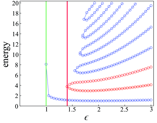
Figure 1: Real eigenvalues from the energy spectrum for the generalized quantum harmonic oscillator from Eqs. (1-2), generated as a function of the parameter $\epsilon$. The vertical line in Red color indicates the exceptional point (EP) at $\epsilon\approx 1.42207$, where two branches from the $1$st- and $2$nd-excited states marked in Red colors merge together.

To find the solutions of the eigenvalue problem with the complex potential, we use connection with a quantum harmonic oscillator and solve Eq. (1) in the Fock state basis. It turns out, that an analytical formula for the matrix element $a_{nm}(\!\epsilon)=\langle m|\mathrm{H}_{\epsilon}|n\rangle$ of $\mathrm{H}_{\epsilon}=\frac{1}{2}\frac{\partial^{2}}{\partial x^{2}}+\frac{V_{\epsilon}(x)}{2}$ can be constructed for any natural number $n$, $m$ and positive $\textstyle\epsilon$. It reads:

$$a_{nm}(\!\epsilon) = {\textstyle{\frac{\sqrt{n(n-1)}}{4}\,\delta_{m,n-2}+\frac{\sqrt{(n+1)(n+2)}}{4}\,\delta_{m,n+2}-\frac{2n+1}{4}\,\delta_{m,n}}}+$$ (4)

$$+ \Big{[}{\textstyle{\frac{1-(-1)^{\widetilde{n}+\widetilde{m}}}{4}}}\cos(\textstyle{{\textstyle{\epsilon}}\frac{\pi}{2}})+\frac{1+(-1)^{\widetilde{n}+\widetilde{m}}}{4}i\sin({\textstyle{\epsilon}}\frac{\pi}{2})\Big{]}\frac{(-1)^{\lfloor\!\frac{n}{2}\!\rfloor+\lfloor\!\frac{m}{2}\!\rfloor}{\textstyle{2^{\widetilde{n}+\widetilde{m}}n!m!}}}{\lfloor\!\frac{n}{2}\!\rfloor!\,\lfloor\!\frac{m}{2}\!\rfloor!}\times$$

$$\times\;\Gamma\!\left({\textstyle{\frac{1+{\textstyle{\epsilon}}+\widetilde{n}+\widetilde{m}}{2}}}\right)F_{\!\!{}_{A}}\!\!\left({\textstyle{\frac{1+{\textstyle{\epsilon}}+\widetilde{n}+\widetilde{m}}{2};-\lfloor\!{\textstyle\frac{n}{2}}\!\rfloor,-\lfloor\!{\textstyle\frac{m}{2}}\!\rfloor;{\textstyle\frac{2\widetilde{n}+1}{2}},{\textstyle\frac{2\widetilde{m}+1}{2}};1,1}}\right)\delta_{m,n}\;,$$

where $\Gamma$ is an Euler gamma function; $F_{\!\!{}_{A}}$ is a Lauricella hypergeometric function; symbol $\lfloor\,\rfloor$ denotes a floor function: $\lfloor\!k\!\rfloor$ is the largest integer not greater than $k$; character tilde $\;\widetilde{}\;$ denotes a binary parity function: $\widetilde{k}$ is 0 for an even $k$ and 1 for an odd $k$. All mathematical formulas needed for derivation of Eq. (4) are presented in Appendix A.

In the analytical expression shown in Eq. (4), the first line comes from the well known formula $2\frac{\partial^{2}}{\partial x^{2}}\,|n\rangle=\sqrt{n(n-1)}\,|n-2\rangle-(2n+1)|n\rangle+\sqrt{(n+1)(n+2)}\,|n+2\rangle$; while the next lines are a combination of parity coefficients and an Erdèlyi formula for the integral $\int_{0}^{\infty}e^{-\lambda x^{2}}H_{\mu_{1}}\!(\beta_{1}x)H_{\mu_{2}}\!(\beta_{2}x)\cdots H_{\mu_{n}}\!(\beta_{n}x)x^{\nu}dx\,,$ Erdelyi . Let us note, that crucial to the derivation are parity properties of Hermite polynomials, e.g., the fact that

$$\int_{-\infty}^{0}e^{-x^{2}}H_{n}(x)H_{m}(x)|x|^{\textstyle{\epsilon}}dx=(-1)^{\widetilde{n}+\widetilde{m}}\int_{0}^{\infty}e^{-x^{2}}H_{n}(x)H_{m}(x)|x|^{\textstyle{\epsilon}}dx.$$ (5)

Whenever $n$ and $m$ have the same parity, the values of $a_{nm}(\epsilon)$, Eq. (4), are real. Otherwise, values $a_{nm}(\epsilon)$ are purely imaginary. Unless $\epsilon$ is an even number, matrix $M_{nn}(\epsilon)$ constructed from elements $a_{nm}(\epsilon)$ is symmetric ($M=M^{\mathrm{T}}$) but non-Hermitian. Numerical diagonalization of $M_{nn}(\epsilon)$, and hence a necessity to truncate the Hilbert space to a finite basis, sets some formal limitation on generality of the results. On the other hand, the method allows for a direct control of precision: truncating basis at $n_{max}$ we automatically know that eigenfunction are expanded into a polynomial of the order $n_{max}$, as

$$\psi_{j}(x,t)=\sum_{k=0}^{n_{max}}a_{jk}u_{k}(x)e^{-\frac{iE_{k}t}{\hbar}}.$$

However, one has to realize that, as long as a finite basis is used, diagonalization of $M_{nn}(\epsilon)$ always leads to discrete spectra. In the general case of a non-truncated basis, there is no way to determine a priori if the spectrum is discrete or even if there exists a square integrable solution of Eq. (1).

Using the matrix elements derived in Eq. (4), we diagonalize the matrix $M_{nn}(\epsilon)$ numerically, having truncated the Fock basis to the first $31$, $51$, or $71$ elements. For low energy states, already the smallest basis of 31 elements gives more than sufficient accuracy. In Fig. 1, we show real eigenvalues of the energy spectrum corresponding to the generalized quantum harmonic oscillator described in Eq. (1). The parameter $\epsilon$ from Eq. (2) is used as a variable. One can see that for $\epsilon<2$ the number of real eigenvalues decreases. When $\epsilon=1$, only the ground state has a real energy; while for parameter $1<\epsilon<2$, the lowest eigenvalues of (1) are real whereas higher eigenvalues might appear in complex conjugate pairs. It was conjured that for $\epsilon\geq 2$ eigenvalues of Eq. (1) are always real; however there is no analytical proof of this statement and although some numerical simulations support the conjecture, others are inconclusive bender . In the following, we focus us on the exceptional point (EP) for the $1$st- and $2$nd- excited states at $\epsilon_{EP}\approx 1.42207$, as indicated by the vertical Red-colored line in Fig. 1. At this EP, two subsequent (up to that point) real eigenvalues start to have the same absolute value but complex conjugate imaginary parts. It is a point at which solutions that break symmetry of the Hamiltonian suddenly appear. In the next Section, we will examine the phase space representation of such eigenfunctions and look for a signature of this exceptional point.

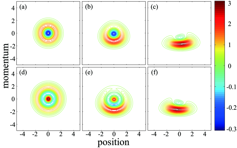
Figure 2: Wigner function distributions for the $1$st- (Upper panel) and $2$nd- (Lower Panel) excited states, at (a): $\epsilon=2.0$, (b): $\epsilon=1.5$, and (c): $\epsilon=1.4$. It is noted that the exceptional point appears at $\epsilon_{EP}\approx 1.42207$.

Figure 3: Wigner function currents for the $1$st- (Upper panel) and $2$nd- (Lower Panel) excited states, at (a): $\epsilon=2.0$, (b): $\epsilon=1.5$, and (c): $\epsilon=1.4$. Here, Arrows denote direction of $\bar{J}_{{\,\psi}}$; while Color of the arrows depends on the norm $N_{\!{}_{J}}$ with dark gray denoting the highest value. Again, the exceptional point happens at $\epsilon_{EP}\approx 1.42207$. Note that depending on the sign of Wigner function, the rotation may be clockwise or counter-clockwise. Insects show the corresponding Wigner function distributions.

III $\mathcal{PT}$-symmetry in Wigner function representation

Phase space wave characteristics of a square-integrable wavefunction $\psi(x,t)$ is often examined through the corresponding Wigner distribution Wigner ; book-phasespace , defined as an integral

$$W_{\!\psi}=W_{\psi}(x,p,t)\mathrel{\mathop{:}}=\frac{1}{2\pi\hbar}\int\psi^{*}(x+{\textstyle{\xi}}/2,t)\psi(x-{\textstyle{\xi}}/2,t)\,e^{i{\xi}p/\hbar}\,d{{\xi}},$$ (6)

where $\psi^{*}$ denotes a complex conjugate of $\psi$. The Wigner function is always real. It is also normalized to $1$ for any normalized $\psi$, but in contrast to proper probability distributions it might take on negative values. The Wigner representation reflects proper probability properties in position and momentum representations simultaneously, and thus is very well suited to reveal the possible symmetries in wavefunctions book-phasespace ; bauke .

In Fig. 2, the Wigner function corresponding to the $1$st- and $2$nd-exited states of Eq. (1) with a $\mathcal{PT}$-symmetric potential given in Eq. (2) are plotted, for $\epsilon=2.0$, $1.5$, and $1.4$, respectively. We start with the case of a quantum harmonic oscillator ($\epsilon=2$), which has all eigenvalues real and the corresponding Wigner functions have a cylindrical symmetry, as shown in Fig. 2(a) and (d). The Wigner function of a harmonic oscillator depends on $r=\sqrt{x^{2}+p^{2}}$ as a $n$th-order Laguerre polynomial suppressed by exponential factor. When $\epsilon\neq 2$, such a cylindrical symmetry vanishes. It is noted from Fig. 1 that the exceptional point for these two states happens at $\epsilon_{EP}\approx 1.42207$. Within the unbroken $\mathcal{PT}$-symmetry phase, $\epsilon>\epsilon_{EP}$, we have the real eigenvalues and the corresponding Wigner functions are symmetric under transformation $x\rightarrow-x$, as shown in Fig. 2(b) and (e) for the $1$st and $2$nd exited states, respectively. However, at the same time, the symmetry $p\rightarrow-p$ that is present in a quantum harmonic oscillator case disappears. Moreover, as expected, the bigger difference between the value of $\epsilon$ and $2$, the less similarity of Wigner distributions to those of a quantum harmonic oscillator is exhibited.

When the $\mathcal{PT}$-symmetry is broken for $\epsilon<\epsilon_{EP}$, the corresponding eigenvalues both for the $1$st and $2$nd exited states not only have non-zero imaginary parts, but also form a complex conjugate pair to each other. In Fig. 2(c) and (f), we plot the Wigner function distributions in such a $\mathcal{PT}$-symmetry-broken phase. As one can see, neither symmetry $p\rightarrow-p$ or $x\rightarrow-x$ is valid. However, this pair of eigenfunctions with the complex conjugates in their eigenvalues are mirror images to each other, with respect to $x=0$. The same mirror-image symmetry holds for any pair of eigenfunctions that have complex conjugate eigenvalues.

In addition to the Wigner function distribution in the phase space, we also introduce a Wigner function flow $\bar{J}_{\psi}$ defining the field $\bar{J}_{\psi}=(J_{x},J_{p})$ as

$$J_{x} = \frac{p}{m}\,W_{\!\psi},\,$$ (7)

$$J_{p} = -\sum_{j=1}^{\infty}\frac{(-i\hbar)^{j-1}}{j!\,2^{j}}\bigg{[}\frac{d^{j}V^{\!*}}{dx^{j}}+(-1)^{j-1}\frac{d^{j}V}{dx^{j}}\bigg{]}\frac{\partial^{j-1}W_{\!\psi}}{\partial p^{j-1}},$$ (8)

where $V$ denotes a potential from the Schrödinger equation that led to eigenfunction $\psi$, and $V^{*}$ is its complex conjugate. In general, a continuity equation is given by

$$\frac{\partial W_{\!\psi}}{\partial t}+\frac{\partial J_{x}}{\partial x}+\frac{\partial J_{p}}{\partial p}=\frac{i}{\hbar}\big{(}V^{\!*}-V\big{)}W_{\!\psi}.$$ (9)

In the Hermitian case, the right-hand-side of Eq. (9) vanishes and in the classical limit of $\hbar\rightarrow 0\;$it is reduced to

$$\frac{\partial W_{\!\psi}}{\partial t}+\frac{p}{m}\,\frac{\partial W_{\!\psi}}{\partial x}-\frac{\partial V}{\partial x}\,\frac{\partial W_{\!\psi}}{\partial p}=0.$$ (10)

This well-known formula determines the classical evolution of the Wigner function. It was first derived by Wigner Wigner and later discussed, e.g., by Wyatt Wyatt . An analogous equation valid when $V^{\!*}\neq V$ reads

$$\frac{\partial W_{\!\psi}}{\partial t}+\frac{p}{m}\,\frac{\partial W_{\!\psi}}{\partial x}-\frac{\partial\mathrm{Re}(V)}{\partial x}\,\frac{\partial W_{\!\psi}}{\partial p}=2\,W_{\!\psi}\lim_{\hbar\rightarrow 0}\frac{\mathrm{Im}(V)}{\hbar}\;,$$ (11)

where $\mathrm{Re}(V)$ and $\mathrm{Im}(V)$ represent the real and imaginary parts of $V\!$, respectively. Unless the imaginary part of potential is proportional to $\hbar$, the right-hand-side in Eq. (11) explodes when $\hbar\rightarrow 0$. If there is no finite limit ${\displaystyle{\lim_{\hbar\rightarrow 0}}}\frac{\mathrm{Im}V}{\hbar}$, we infer from the Bohr rule that there is no classical system governed by a Hamiltonian $\frac{p^{2}}{2m}+V$.

There is an underlying assumption in formulation of Eq. (8), that at every point $x$ potential $V(x)$ can be expanded into a power series with an infinite radius of convergence. When it is not the case, relation shown in Eq. (9) still holds, but one needs to calculate $J_{p}$ as a full integral

$$J_{p}\!=\!\!\int\!\!\!\frac{d\xi}{2\pi{\textstyle{i}}}\,e^{i\xi p/\hbar}\,\psi^{*}(x\!+\!{\textstyle{\frac{\xi}{2}}})\psi(x\!-\!{\textstyle{\frac{\xi}{2}}})\!\bigg{[}\dfrac{V\!(x\!-\frac{\xi}{2})\!-\!V\!(x)}{\xi}\!-\!\frac{V^{\!*}\!(x\!+\frac{\xi}{2})\!-\!V^{*}\!(x)}{\xi}\!\bigg{]}.$$ (12)

Here, both $\dfrac{V\!(x\!-\frac{\xi}{2})\!-\!V\!(x)}{\xi}$ and $\dfrac{V\!(x\!+\frac{\xi}{2})\!-\!V\!(x)}{\xi}\;$ have finite values in a limit of $\xi\rightarrow 0$, which means that $J_{p}$ in Eq. (12) is a well defined continuous function on $(x,p)$. Defined by Eqs. (7) and (12) Wigner function flow is a generalization of formulas used to study phase-space dynamics in Wigner representation Wyatt ; bauke ; steuer to the case of complex potential. Similarly, the continuity equation for the Wigner distribution shown in Eq. (9), along with the definition in Eq. (12), can be applied to an arbitrary complex potential, which is not necessary Hermitian or a $\mathcal{PT}$-symmetric one.

For the convenience of notation, from now on we set $\hbar=1$. We calculate the Wigner function flow $\bar{J}_{\psi}$ for the eigenstates of Eq. (1) using a potential $V=\frac{V_{\epsilon}(x)}{2}$ defined in Eq. (2). In Fig. 3, the streamline plots of $\;\bar{J}_{\!\psi}$ corresponding to the $1$st- and $2$nd-excited states are depicted, again for $\epsilon=2.0$, $1.5$, and $1.4$, respectively. In the figures, the Wigner distribution is plotted as the background. A color of the arrows depends on the norm $N_{\!{}_{J}}=\sqrt{J_{x}^{2}+J_{p}^{2}}\;$, varying from white-color (for $N_{\!{}_{J}}=0$) to dark-color (for large $N_{\!{}_{J}}$). As illustrated in Fig. 3(a) and (d), streamlines corresponding to the harmonic oscillator form perfect circles. The streamlines rotate clockwise or counterclockwise, depending on the sign of the Wigner function. In general, the sign of $J_{x}$ depends on the sign of the Wigner function and momentum: $\mathrm{sgn}(J_{x})=\mathrm{sgn}(pW_{\!\psi})$, and $\;\bar{J}_{\!\psi}$ vanishes at the points where the Wigner function vanishes.

As demonstrated in Fig. 3, for $\epsilon<2$ the streamlines are no longer perfect circles. However, the deformation in the streamlines just reflects changes in the Wigner function, but the characteristics of the field is not alerted qualitatively. As long as the $\mathcal{PT}$-symmetry is unbroken, these streamlines still form closed loops and their orientation depends on the sign of the Wigner distribution, see Fig. 3(b) and (e). However, when the $\mathcal{PT}$-symmetry is broken, as shown in Fig. 3(c) and (f), a quantitative difference will be revealed for these Wigner function currents by the means of Gauss-Ostrogradsky theorem.

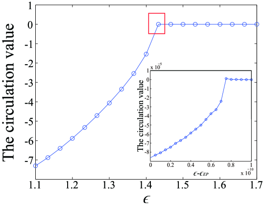
Figure 4: The circulation value, i.e., the integral calculated by Eq. (14) for the Wigner function flow from the $1$st-excited as a function of the parameter $\epsilon$. Markers in circles denote numerically values. Here, the exceptional point happens at $\epsilon_{EP}\approx 1.42207$. One can see that integral is equal to zero when $\epsilon\geq\epsilon_{EP}$. Inset shows the enlarged area in the vicinity of the exception point.

IV Wigner Function Flow at the exceptional points

The divergence theorem, i.e., Gauss-Ostrogradsky theorem, states that the flux of a vector field through a closed surface is equal to the volume integral of the divergence over the region inside the surface Tromba ; Jackson . It allows us to calculate the flux through volume or surface integrals and quantitatively distinguishes cases of unbroken and broken $\mathcal{PT}$-symmetry. To apply the divergence theorem, we introduce a three dimensional (3D) field $\bm{\mathcal{J}_{\!\!\scriptscriptstyle{3}\,}}\mathrel{\mathop{:}}=(W_{\!\psi},J_{x},J_{p})$, and rewrite the continuity equation for the Wigner function in Eq. (9) by this 3D field. In this notation, Eq. (9) is expressed simply as

$$\nabla\cdot\bm{\mathcal{J}_{\!\!\scriptscriptstyle{3}\,}}=2W_{\!\psi}\mathrm{Im}V\,.$$

From the divergence theorem we infer that a flux ${\bm{\psi_{\mathcal{J}_{\!\scriptscriptstyle{3}}}}}$ of the field $\bm{\mathcal{J}_{\!\!\scriptscriptstyle{3}}}$ through a surface $S$ enclosing volume ${\mathrm{U}}$ can be calculated by taking a volume integral of $\,2W_{\!\scriptstyle{\Psi}}\mathrm{Im}V$ over ${\mathrm{U}}$:

$${\bm{\psi_{\mathcal{J}_{\!\scriptscriptstyle{3}}}}}=\oiint_{\mathrm{S}}\bm{\mathcal{J}_{\!\!\scriptscriptstyle{3}}}d\mathrm{S}=\iiint_{\mathrm{U}}(\nabla\cdot\bm{\mathcal{J}_{\!\!\scriptscriptstyle{3}}})dtdxdp=2\iiint_{\mathrm{U}}\mathrm{Im}V\,W_{\!\scriptstyle{\Psi}}\,dtdxdp\,.$$ (13)

From Eq. (13), it is clear that the flux ${\bm{\psi_{\mathcal{J}_{\!\scriptscriptstyle{3}}}}}=0\,$ when the imaginary part of $V$ vanishes. It follows, that the flux ${\bm{\psi_{\mathcal{J}_{\!\scriptscriptstyle{3}\,}}}}$ vanishes for all Hermitian Hamiltonians.

Whenever the Wigner function does not depend on time, i.e., $\frac{\partial W\!(x,p,t)}{\partial t}=0$, a flux ${\bm{\psi_{\mathcal{J}_{\!\scriptscriptstyle{3}}}}}$ of the field $\bm{\mathcal{J}_{\!\!\scriptscriptstyle{3}}}$ through a surface $S$ for a unit time can be calculated as a two-dimensional (2D) integral $\iint 2W_{\!\scriptstyle{\Psi}}\mathrm{Im}(V)dxdp$. Here, a product of the Wigner distribution and the imaginary part of potential $V$, can be viewed as a charge/probability density determining behavior of a field ${\bm{{\mathcal{J}_{\!\scriptscriptstyle{3}}}}}$. Note that, as long as $V$ is antisymmetric under the transformation $x\rightarrow-x$, the corresponding value of $W_{\!\scriptstyle{\Psi}}\mathrm{Im}(V)$ is zero whenever the Wigner function is symmetric under the same transformation. It also shows that a flux ${\bm{\psi_{\mathcal{J}_{\!\scriptscriptstyle{3}}}}}$ is non-zero only under the presence of a non-Hermitian part of Hamiltonian and only when a $\mathcal{PT}$-symmetry of a given solution is broken. This fact provides a quantitative measure, which allows us to distinguish the cases of broken and unbroken $\mathcal{PT}$ symmetry.

Alternatively, instead of treating time parameter $t$ as a third dimension, one can also stay in the 2D case by defining an auxiliary field ${\bm{\mathcal{I}_{2}}}=(-J_{p},J_{x})$. Now, let us consider a surface $D$ that has a boundary $C=\partial D$. In 2D, the circulation of a field ${\bm{\mathcal{I}_{2}}}$ along a curve $C$ can be calculated as an area integral over $D$. Again, from the divergence theorem we know that a circulation from the field ${\bm{\psi_{{\bm{\mathcal{I}_{2}}}}}}$ of the field ${\bm{\mathcal{I}_{2}}}$ along $C$ can be calculated as a two-dimensional area integral of $\mathrm{Im}(V)W\!(x,p,t)-\frac{\partial W\!(x,p,t)}{\partial t}$ over $D$, or equivalently:

$$\oint_{C}{\bm{\mathcal{I}_{2}}}\,dC = \int\!\!\!\!\int_{\!D}\left(\frac{\partial\mathcal{I}_{x}}{\partial p}-\frac{\partial\mathcal{I}_{p}}{\partial x}\right)dxdp=\int\!\!\!\!\int_{\!D}\!\left(\!2W_{\!\scriptstyle{\Psi}}\mathrm{Im}V-\frac{\partial W_{\!\scriptstyle{\Psi}}}{\partial t}\!\right)\!dxdp\,.$$ (14)

Figure 4 shows the circulation value, the integral from Eq. (14) versus the parameter $\epsilon$ for the $1$st-excited state of our modal system with $\mathcal{PT}$-symmetry in Eqs. (1-2). Here, the curve $C$ encircles the area $D$, which is taken large enough to ensure that the integral value does not change for any more expansion. One can find that when $\epsilon\geq\epsilon_{EP}\approx 1.42207$, the circulation value is always zero, no matter the symmetry in the Wigner function distribution sustains shown in Fig. 2. However, across this exceptional point, $\epsilon_{EP}$, the circulation value has a non-zero term, which reflects a broken $\mathcal{PT}$-symmetry phase. Moreover, we check this circulation value in the vicinity of $\epsilon_{EP}$ to $10$th decimal places, as shown in the Insect of Fig. 4. With this numerical check, we can confirm that the phase transition in our $\mathcal{PT}$-symmetric system is a continuous function of the parameter $\epsilon$, which implies a second-order phase transition.

V Conclusions

We present a phase-space study of a non-Hermitian system deriving a continuity equation for the Wigner distribution and arbitrary complex potential, defining a Wigner function flow accordingly. In particular, we reveal how a $\mathcal{PT}$ symmetry-breaking manifests itself in the phase-space representation. A quantitative measure on the circulation value for the Wigner function flow shows that the phase transition in the vicinity of exception point (EP) is a continuous function of the system parameter. Our study in phase space representation indicates that a $\mathcal{PT}$-symmetric phase transition is a second-order phase transition.

Appendix A

In this Appendix, we provide the formula for the Lauricella hypergeometric function shown in Eq. (4). With the basic properties of Hermite polynomials, it is easy to check that

$$-2\frac{\partial^{2}}{\partial x^{2}}\,|n\rangle=(2n+1)|n\rangle-\sqrt{n(n-1)}\,|n-2\rangle-\sqrt{(n+1)(n+2)}\,|n+2\rangle\,.$$ (1)

To calculate $\langle m|V_{\epsilon}(x)|n\rangle$ it is useful to note that depending on the parity of $n$ and $m$

$$\int_{-\infty}^{0}e^{-x^{2}}H_{m}(x)H_{n}(x)|x|^{\textstyle{\epsilon}}dx=\pm\int_{0}^{\infty}e^{-x^{2}}H_{m}(x)H_{n}(x)|x|^{\textstyle{\epsilon}}dx\;.$$

Thus, for a given $\epsilon$, the value of an integral

$$\int_{{}_{\textstyle\mathbb{R}}}\!\!e^{-x^{2}}\!H_{m}(x)H_{n}(x)V_{\epsilon}(x)\,dx = \int_{-\infty}^{0}e^{-x^{2}}H_{m}(x)H_{n}(x)|x|^{\textstyle{\epsilon}}\big{[}\cos(\frac{\pi}{2}{\textstyle{\epsilon}})-i\sin(\frac{\pi}{2}{\textstyle{\epsilon}})\big{]}dx+$$

$$+ \int_{0}^{\infty}e^{-x^{2}}H_{m}(x)H_{n}(x)|x|^{\textstyle{\epsilon}}\big{[}\cos(\frac{\pi}{2}{\textstyle{\epsilon}})+i\sin(\frac{\pi}{2}{\textstyle{\epsilon}})\big{]}dx$$

is determined by an integral (2) defined below. It was shown by Erdèlyi Erdelyi that

$$2\int_{0}^{\infty} \!\!\!\!\!\!e^{-x^{2}}H_{\mu}(x)H_{\nu}(x)x^{\textstyle{\epsilon}}dx=h_{\mu}h_{\nu}\Gamma\big{(}{\textstyle{1+\frac{\textstyle{\epsilon}}{2}-\frac{(-1)^{\mu}+(-1)^{\nu}}{4}}}\big{)}\times$$ (2)

$$\times\,F_{A}\big{(}{\textstyle{1+\frac{\textstyle\epsilon}{2}-\frac{(-1)^{\mu}+(-1)^{\nu}}{4};\frac{\{\mu\}-\mu}{2};\frac{\{\nu\}-\nu}{2};1-\frac{(-1)^{\mu}}{2};1-\frac{(-1)^{\nu}}{2};1,1}}\big{)}\,,$$

where $\Gamma(.)$ is an Euler gamma function, $F_{A}(.)$ denotes a Lauricella hypergeometric function and parameters $h_{\mu}$, $h_{\nu}$ are defined as:

$$h_{\mu}=\begin{cases}(-1)^{\frac{\mu}{2}}\,\mu!\left[\left(\frac{\mu}{2}\right)!\right]^{-1};&\text{for even}\;\mu\\ (-1)^{\frac{\mu+1}{2}}\,2\mu!\left[\left(\frac{\mu-1}{2}\right)!\right]^{-1};&\text{for odd}\;\mu\end{cases}$$

For different parities of $\mu$ and $\nu$ one obtains:

$$\!\!\!\!\!\!\!\!\int_{0}^{\infty}\!\!\!e^{-x^{2}}H_{2r}(x\!)H_{2\!s}(x\!)\,x^{\textstyle{\epsilon}}dx=\frac{(-1)^{r+s}(\!2r\!)!(\!2s\!)!}{2r!s!}\,{\displaystyle{\Gamma}}\!\left(\textstyle{\frac{{\textstyle{\epsilon}}+1}{2}}\right)F_{A}\!\!\left({\textstyle{\frac{{\textstyle{\epsilon}}+1}{2}}}\,;-r,-s\,;{\textstyle\frac{1}{2}},{\textstyle\frac{1}{2}}\,;1,1\right),$$ (3)

$$\!\!\!\!\!\!\!\!\int_{0}^{\infty}\!\!\!e^{-x^{2}}H_{2r}(x\!)H_{2\!s+1}\!(x\!)\,x^{\textstyle{\epsilon}}dx=\frac{(-1)^{r+s}(\!2r\!)!(\!2s+1\!)!}{r!s!}\,\Gamma\!\left(\textstyle{\frac{{\textstyle{\epsilon}}+2}{2}}\right)F_{A}\!\!\left({\textstyle{\frac{{\textstyle{\epsilon}}+2}{2}}}\,;-r,-s\,;{\textstyle\frac{1}{2}},{\textstyle\frac{3}{2}}\,;1,1\right),$$ (4)

$$\!\!\!\!\!\!\!\!\int_{0}^{\infty}\!\!\!e^{-x^{2}}H_{2r+1}\!(x\!)H_{2\!s+1}\!(x\!)\,x^{\textstyle\epsilon}dx=\frac{2(-1)^{r+s}(\!2r+1\!)!(\!2s+1\!)!}{r!s!}\,\Gamma\!\left(\textstyle{\frac{{\textstyle{\epsilon}}+3}{2}}\right)F_{A}\!\!\left({\textstyle{\frac{{\textstyle{\epsilon}}+3}{2}}}\,;-r,-s\,;{\textstyle\frac{3}{2}},{\textstyle\frac{3}{2}}\,;1,1\right),$$

Relation (2) is a special case of more general formula for an integral $\int_{0}^{\infty}e^{-\lambda x^{2}}H_{\mu_{1}}\!(\beta_{1}x)H_{\mu_{2}}\!(\beta_{2}x)\cdots H_{\mu_{n}}\!(\beta_{n}x)x^{\nu}dx$, which we don’t rewrite here because of its length. Lauricella hypergeometric function is defined as

$$F_{A}^{(n)}(a;b_{1},...,b_{2};c_{1},...,c_{n};x_{1},...,x_{n})=\!\!\!\!\!\!\sum_{i_{1},...,i_{n}=0}^{\infty}\!\!\!\frac{\bm{(}a\bm{)}_{i_{1}+...+i_{n}}{\bm{(}}b_{1}\bm{)}_{i_{1}}\cdots\bm{(}b_{n}\bm{)}_{i_{n}}}{\bm{(}c_{1}\bm{)}_{i_{1}}\cdots\bm{(}c_{n}\bm{)}_{i_{n}}i_{n}!\cdots i_{n}!}\,x_{1}^{i_{1}}\cdots x_{n}^{i_{n}}$$ (5)

with $\,{\bm{(}}.\bm{)}_{k}\,$ being a Pochhammer symbol, i.e., $\,{\bm{(}}a\bm{)}_{k}=a(a+1)\cdots(a+k-1)$. In our case, $n=2$ and $F_{A}(.)$ are of the form

$$F_{A}\left({\textstyle{\frac{{\textstyle{\epsilon}}+1}{2}}}\,;-r,-s\,;{\textstyle\frac{1}{2}},{\textstyle\frac{1}{2}}\,;1,1\right)=\sum_{i_{1},i_{2}=0}^{\infty}\frac{\bm{(}{\textstyle{\frac{{\textstyle{\epsilon}}+1}{2}}}\bm{)}_{i_{1}+i_{2}}{\bm{(}}-r\bm{)}_{i_{1}}\bm{(}-s\bm{)}_{i_{2}}}{\bm{(}\frac{1}{2}\bm{)}_{i_{1}}\bm{(}\frac{1}{2}\bm{)}_{i_{2}}\,i_{1}!\,i_{2}!}\,.$$

Because $r$ and $s$ are natural numbers there will be always a finite number of terms in the sum as ${\bm{(}}-r\bm{)}_{k}=0\quad$ for $\,k\geq r+1\,,$ so

$$\sum_{i_{1},i_{2}=0}^{\infty}\frac{\bm{(}{\textstyle{\frac{{\textstyle{\epsilon}}+1}{2}}}\bm{)}_{i_{1}+i_{2}}{\bm{(}}-r\bm{)}_{i_{1}}\bm{(}-s\bm{)}_{i_{2}}}{\bm{(}\frac{1}{2}\bm{)}_{i_{1}}\bm{(}\frac{1}{2}\bm{)}_{i_{2}}\,i_{1}!\,i_{2}!}=\sum_{i_{1},i_{2}=0}^{r,s}\frac{\bm{(}{\textstyle{\frac{{\textstyle{\epsilon}}+1}{2}}}\bm{)}_{i_{1}+i_{2}}{\bm{(}}-r\bm{)}_{i_{1}}\bm{(}-s\bm{)}_{i_{2}}}{\bm{(}\frac{1}{2}\bm{)}_{i_{1}}\bm{(}\frac{1}{2}\bm{)}_{i_{2}}\,i_{1}!\,i_{2}!}\,=$$

$$=1+\sum_{i_{1}=1}^{r}\frac{\bm{(}{\textstyle{\frac{{\textstyle{\epsilon}}+1}{2}}}\bm{)}_{i_{1}}{\bm{(}}-r\bm{)}_{i_{1}}}{\bm{(}\frac{1}{2}\bm{)}_{i_{1}}\,i_{1}!}\,+\sum_{i_{2}=1}^{s}\frac{\bm{(}{\textstyle{\frac{{\textstyle{\epsilon}}+1}{2}}}\bm{)}_{i_{2}}{\bm{(}}-s\bm{)}_{i_{1}}}{\bm{(}\frac{1}{2}\bm{)}_{i_{2}}\,i_{2}!}\,+\sum_{i_{1},i_{2}=1}^{r,s}\frac{\bm{(}{\textstyle{\frac{{\textstyle{\epsilon}}+1}{2}}}\bm{)}_{i_{1}+i_{2}}{\bm{(}}-r\bm{)}_{i_{1}}\bm{(}-s\bm{)}_{i_{2}}}{\bm{(}\frac{1}{2}\bm{)}_{i_{1}}\bm{(}\frac{1}{2}\bm{)}_{i_{2}}\,i_{1}!\,i_{2}!}.\,$$

We can use following formula:

$${\bm{(}}-r\bm{)}_{k}=(-r)(-r+1)\cdots(-r+k-1)=(-1)^{k}\,r\,(r-1)\cdots(r-(k-1))=\frac{(-1)^{k}\,r!}{(r-k)!},$$

and rewrite

$$\sum_{i_{1}=1}^{r}\frac{\bm{(}{\textstyle{\frac{{\textstyle{\epsilon}}+1}{2}}}\bm{)}_{i_{1}}{\bm{(}}-r\bm{)}_{i_{1}}}{\bm{(}\frac{1}{2}\bm{)}_{i_{1}}\,i_{1}!}\,=r!\sum_{i_{1}=1}^{r}\frac{(-1)^{i_{1}}\bm{(}{\textstyle{\frac{{\textstyle{\epsilon}}+1}{2}}}\bm{)}_{i_{1}}}{\bm{(}\frac{1}{2}\bm{)}_{i_{1}}\,i_{1}!(r-i_{1})!}\,=r!\sum_{i_{1}=1}^{r}\frac{(-1)^{i_{1}}\prod_{k=1}^{i_{1}}(\epsilon+2k-1)}{(2i_{1}-1)!!\,i_{1}!\,(r-i_{1})!},\,$$ (6)

where we use also the facts that:

$${\bm{\Big{(}}}\frac{1}{2}\bm{\Big{)}}_{n} = \frac{(2n-1)!!}{2^{n}},$$

and

$${\bm{\Big{(}}}\frac{\epsilon+1}{2}\bm{\Big{)}}_{n} = \frac{(\epsilon+1)(\epsilon+3)\cdots(\epsilon+2n-1)}{2^{n}}=\frac{1}{2^{n}}\,{\displaystyle\prod_{k=1}^{n}(\epsilon+2k-1)}.$$

Similarly, we have

$$\sum_{i_{2}=1}^{s}\frac{\bm{(}{\textstyle{\frac{{\textstyle{\epsilon}}+1}{2}}}\bm{)}_{i_{2}}{\bm{(}}-s\bm{)}_{i_{2}}}{\bm{(}\frac{1}{2}\bm{)}_{i_{2}}\,i_{2}!}\,=s!\,\sum_{i_{1}=1}^{s}\frac{(-1)^{i_{2}}\prod_{k=1}^{i_{2}}(\epsilon+2k-1)}{(2i_{2}-1)!!\,i_{2}!\,(r-i_{2})!},\,$$ (7)

and

$$\sum_{i_{1},i_{2}=1}^{r,s}\frac{\bm{(}{\textstyle{\frac{{\textstyle{\epsilon}}+1}{2}}}\bm{)}_{i_{1}+i_{2}}{\bm{(}}-r\bm{)}_{i_{1}}{\bm{(}}-s\bm{)}_{i_{2}}}{\bm{(}\frac{1}{2}\bm{)}_{i_{1}}\bm{(}\frac{1}{2}\bm{)}_{i_{2}}\,i_{1}\,i_{2}!}\,=s!\,\sum_{i_{1}=1}^{s}\frac{(-1)^{i_{2}}\prod_{k=1}^{i_{2}}(\epsilon+2k-1)}{(2i_{2}-1)!!\,i_{2}!\,(r-i_{2})!}.\,$$ (8)

Combining Eqs. (6), (7) and (8) we can rewrite $F_{A}\left({\textstyle{\frac{{\textstyle{\epsilon}}+1}{2}}}\,;-r,-s\,;{\textstyle\frac{1}{2}},{\textstyle\frac{1}{2}}\,;1,1\right)$ in a convenient form of finite sums.

Using facts that

$${\bm{\Big{(}}}\frac{3}{2}\bm{\Big{)}}_{n}=\frac{(2n-1)!!}{2^{n+1}}\,,\qquad\mathrm{and}$$

$${\bm{\Big{(}}}\frac{\epsilon+2}{2}\bm{\Big{)}}_{n}=\frac{(\epsilon+2)(\epsilon+4)\cdots(\epsilon+2n)}{2^{n}}=\frac{1}{2^{n}}\,{\displaystyle\prod_{k=1}^{n}(\epsilon+2k)}\,,$$

$${\bm{\Big{(}}}\frac{\epsilon+3}{2}\bm{\Big{)}}_{n}=\frac{(\epsilon+3)(\epsilon+5)\cdots(\epsilon+2n+1)}{2^{n}}=\frac{1}{2^{n}}\,{\displaystyle\prod_{k=1}^{n}(\epsilon+2k+1)}\,,$$

analogues formulas for two other functions $F_{A}\Big{(}{\textstyle{\frac{{\textstyle{\epsilon}}+2}{2}}}\,;-r,-s\,;{\textstyle\frac{1}{2}},{\textstyle\frac{3}{2}}\,;1,1\Big{)}$ and $F_{A}\Big{(}{\textstyle{\frac{{\textstyle{\epsilon}}+3}{2}}}\,;-r,-s\,;{\textstyle\frac{3}{2}},{\textstyle\frac{3}{2}}\,;1,1\Big{)}$ are obtained. Together they simplify calculation of elements $a_{nm}(\epsilon)$,Eq. (4), considerably. In principle, finding these elements can be done by hand without any aid of numerics.

References

• (1) C. M. Bender, S. Boettcher, “Real spectra in non-Hermitian Hamiltonians having PT symmetry,” Phys. Rev. Lett. 80, 5243, (1998).
• (2) C. M. Bender, S. Boettcher and P. N. Meisinger, “PT-symmetric quantum mechanics,” J. Math. Phys. 40, 2201-2229, (1999).
• (3) C. M. Bender, D. C. Brody, and H. F. Jones, “Complex extension of quantum mechanics,” Phys. Rev. Lett. 89, 270401, (2002).
• (4) Y.-C. Lee, M.-H. Hsieh, S. T. Flammia, and R.-K. Lee, “Local $\mathcal{PT}$ symmetry violates the no-signaling principle,” Phys. Rev. Lett. 112, 130404 (2014).
• (5) K. G. Makris, R. El-Ganainy, D. N. Christodoulides, and Z. H. Musslimani, “Beam dynamics in $\mathcal{PT}$ symmetric optical lattices,” Phys. Rev. Lett. 100, 103904 (2008).
• (6) A. Guo, G. J. Salamo, D. Duchesne, R. Morandotti, M. Volatier-Ravat, V. Aimez, G. A. Siviloglou, and D. N. Christodoulides, “Observation of $\mathcal{PT}$-symmetry breaking in complex optical potentials,” Phys. Rev. Lett. 103, 093902 (2009).
• (7) C. E. Rüter, K. G. Makris, R. El-Ganainy, D. N. Christodoulides, M. Segev, and D. Kip, “Observation of parity-time symmetry in optics,” Nature Phys. 6, 192 (2010).
• (8) Y.-C. Lee, J. Liu, Y.-L. Chuang, M.-H. Hsieh, and R.-K. Lee, “Passive $\mathcal{PT}$-symmetric couplers without complex optical potentials,” Phys. Rev. A 92, 053815 (2015).
• (9) S.V. Suchkov, A.A. Sukhorukov, J. Huang, S.V. Dmitriev, C. Lee, and Yu. S. Kivshar, “Nonlinear switching and solitons in PT-symmetric photonic systems,” Laser Photonics Rev. 10, 177 (2016).
• (10) B. Peng, S. K. Ozdemir, S. Rotter, H. Yilmaz, M. Liertzer, F. Monifi, C. M. Bender, F. Nori, and L. Yang, “Loss-induced suppression and revival of lasing,” Science 346, 328 (2014).
• (11) L. Feng, Z.J. Wong, R.-M. Ma, Y. Wang, X. Zhang, “Single-mode laser by parity-time symmetry breaking,” Science 346, 972 (2014).
• (12) M. Znojil, “Time-dependent version of crypto-Hermitian quantum theory,” Phys. Rev. D 78, 085003, (2008).
• (13) M. Znojil, “Three-Hilbert-space formulation of quantum mechanics,” SIGMA 5 001(2009).
• (14) To define an operator one has to state explicitly its domain (usually a vector space), to talk about hermiticity also a definition of an inner product on this space is required. The spectral theorem makes a classification of finite-dimensional cases fairly simple: if an operator $\hat{M}$ is diagonalizable and has purely real eigenvalues, then there exists a scalar product in respect to which $\hat{M}$ is Hermitian. If an operator $\hat{M}$ is diagonalizable but has some non-real eigenvalues, it can always be decomposed into a sum of two, mutually commuting, hermitian operators. In the infinite-dimensional case, the linear independence of vectors is no longer sufficient to guarantee that a mapping between basis corresponding to different scalar products is continuous. A much stronger condition that there are no limit points in the set of eigenvectors has to be fulfilled.
• (15) A. Erdèlyi, “Über einige bestimmte Integrale, in denen die Whittakerschen $M_{k,m}$-Funktionen auftreten,” Mathematische Zeitschrift (Berlin, Heidelberg) $\mathbf{43}$, 693, (1936).
• (16) E. Wigner, “On the quantum correction for thermodynamic equilibrium,” Phys. Rev. 40, 749 (1932).
• (17) Quantum Mechanics in Phase Space, edited by C.K. Zachos, D. B. Fairlie, and T. L. Curtright (World Scientific, 2005).
• (18) H. Bauke and N. R. Itzhak, “Visualizing quantum mechanics in phase space,” arXiv: 1101.2683v1 (2011).
• (19) R. E. Wyatt, Quantum Dynamics with Trajectories (Springer, 2005).
• (20) O. Steuernagel, D. Kakofengitis and G. Ritter, “Wigner flow reveals topological order in quantum phase space dynamics,” Phys. Rev. Lett. 110, 030401 (2013).
• (21) M. Veronez and M. A. M. de Aguiar “Phase space flow in the Husimi representation,” J. Phys. A: Math. Theor. 46, 485304 (2013).
• (22) J. E. Marsden and A. Tromba, Vector Calculus, Ch. 8 (W. H. Freeman, 2011).
• (23) J. D. Jackson, Classical Electrodynamics, Ch. 1 (John Wiley & Sons, 1998).