Bayesian functional linear regression
with sparse step functions

Abstract

The functional linear regression model is a common tool to determine the relationship between a scalar outcome and a functional predictor seen as a function of time. This paper focuses on the Bayesian estimation of the support of the coefficient function. To this aim we propose a parsimonious and adaptive decomposition of the coefficient function as a step function, and a model including a prior distribution that we name Bayesian functional Linear regression with Sparse Step functions (Bliss). The aim of the method is to recover areas of time which influences the most the outcome. A Bayes estimator of the support is built with a specific loss function, as well as two Bayes estimators of the coefficient function, a first one which is smooth and a second one which is a step function. The performance of the proposed methodology is analysed on various synthetic datasets and is illustrated on a black Périgord truffle dataset to study the influence of rainfall on the production.

MSC 2010 subject classifications: Primary 62F15; Secondary 62J05.

Keywords: Bayesian regression, function data, support estimate, parsimony.

1 Introduction

Consider that one wants to explain the final outcome $y$ of a process along time (for instance the amount of some agricultural production) thanks to what happened during the whole history (for instance, the rainfall history, or temperature history). Among the statistical learning methods, functional linear models (Ramsay and Silverman, , 2005) aim at predicting a scalar $y$ based on covariates $x_{1}(t),x_{2}(t),\ldots,x_{q}(t)$ lying in a functional space, $L^{2}(\mathcal{T})$ say, where $\mathcal{T}$ is an interval of $\mathbb{R}$. If $x_{q+1},\ldots,x_{p}$ are additional scalar covariates, the outcome $y$ is predicted linearly with

$$\widehat{y}=\mu+\int_{\mathcal{T}}\beta_{1}(t)x_{1}(t)\mathrm{d}t+\cdots+\int_{\mathcal{T}}\beta_{q}(t)x_{q}(t)\mathrm{d}t+\beta_{q+1}x_{q+1}+\cdots+\beta_{p}x_{p},$$ (1)

where $\mu$ is the intercept, $\beta_{1}(t),\ldots,\beta_{q}(t)$ the coefficient functions, and $\beta_{q+1},\ldots,\beta_{p}$ the other (scalar) coefficients. In this framework the functional covariates $x_{j}(t)$ and the unknown coefficient functions $\beta_{j}(t)$ lie in the $L^{2}(\mathcal{T})$ functional space, thus we face a nonparametric problem. Standard methods (Ramsay and Silverman, , 2005) for estimating the $\beta_{j}(t)$’s, $1\leq j\leq q$, are based on the expansion onto a given basis of $L^{2}(\mathcal{T})$. See Reiss et al., (2016) for a comprehensive scan of the methodology. A question which arises naturally in many applied contexts is the detection of periods of time which influence the most the final outcome $y$. Note that each integral in (1) is a weighted average of the whole trajectory of $x_{j}(t)$, and does not identify any specific impact of local period of the process. These time periods might vary from one covariates to another. For instance, in agricultural science, the final outcome may depend on the amount of rainfall during a given period (e.g., to prevent rotting), and the temperature during another (e.g., to prevent freezing). Standard methods do not answer the above question, namely to recover the support of the coefficient functions $\beta_{j}(t)$ with the noticeable exception of Picheny et al., (2016).

Unlike the scalar-on-image models, we focus here on one-dimensional functional covariates. When $\mathcal{T}$ is not a one dimensional space, the problem becomes much more complex. The functional covariates and the coefficient functions are all discretized, e.g. via the pixels of the images, see Goldsmith et al., (2014); Li et al., (2015); Kang et al., (2016). In these two- or three-dimensional problems, because of the curse of dimensionality, the points which are included in the support of the coefficient functions follow a parametric distribution, namely an Ising model. One important issue solved by these authors is the sensitivity of the parameter estimate of the Ising model in the neighborhood of the phase transition.

When $\mathcal{T}$ is a one dimensional space, we can build nonparametric estimates. In this vein, using the $L^{1}$-penalty to achieve parsimony, the Flirti method of James et al., (2009) obtains an estimate of the $\beta_{j}(t)$’s assuming they are sparse functions with sparse derivatives. Nevertheless Flirti is difficult to calibrate: its numerical results depend heavily on tuning parameters. From our experience, Flirti’s estimate is so sensitive to the values of the tuning parameters that we can miss the range of good values with cross-validation. The authors propose to rely on cross-validation to set these tuning parameters. But, by definition, cross-validation assesses the predictive performance of a model, see Arlot and Celisse, (2010) and the many references therein. And, of course, optimizing the performance regarding the prediction of $y$ does not provide any guaranty regarding the support estimate. Zhou et al., (2013) propose a two-stage method to estimate the coefficient function. Preliminarily, $\beta(t)$ is expanded onto a B-spline basis to reduce the dimension of the model. The first stage estimates the coefficients of the truncated expansion onto the basis using a lasso method to find the null intervals. Then, the second stage refines the estimation of the null intervals and estimates the magnitude of $\beta(t)$ for the rest of the support. Another approach to obtain parsimony is to rely on Fused lasso (Tibshirani et al., , 2005): if we discretize the covariate functions and the coefficient function as described in James et al., (2009), the penalization of Fused lasso induces parsimony in the coefficients. But, once again the calibration of the penalization is performed using cross-validation which targets predictive perfomance rather than the accuracy of the support estimate.

In this paper, we propose Bayesian estimates of both the supports and the coefficient functions $\beta_{i}(t)$’s. To keep the dimension of the parameter as low as possible, we stay with the simplest and the most parsimonious shape of the coefficient function over its support. Hence, conditionally on the support, the coefficient functions $\beta_{j}(t)$’s are supposed to be step function (piecewise constant function can be described with a minimal number of parameters). We can decompose any step function $\beta(t)$ as

$$\beta(t)=\sum_{k=1}^{K}\beta^{\ast}_{k}\frac{1}{|\mathcal{I}_{k}|}\mathbf{1}\{t\in\mathcal{I}_{k}\}$$

where $\mathcal{I}_{1},\ldots,\mathcal{I}_{K}$ are intervals of $\mathcal{T}$, $|\mathcal{I}_{k}|$ is the length of the interval $\mathcal{I}_{k}$ and $\beta^{\ast}_{k}$ are the coefficients of the expansion. The support is the union of all $\mathcal{I}_{k}$’s if the coefficients $\beta^{\ast}_{k}$ are non null. Period of times which does not influence the outcome are outside the support. The above model has another advantage: such step functions change values abruptly from $0$ to a non null value. Hence their supports are relatively clear. On the contrary, if we have at our disposal a smooth estimate of a coefficient function $\beta_{j}(t)$ in the model given by (1), the support of the estimate is the whole $\mathcal{T}$ and we have to find regions where the estimate is not significantly different from $0$. Moreover, with a full Bayesian procedure, we can evaluate the uncertainty on the estimates of the support and the values of the coefficient functions.

The paper is organized as follows. Section 2 presents the Bayesian modelling, including the prior distribution in 2.2, the support estimate in 2.3 and the coefficient function estimate in 2.4. Section 3 is devoted to the study of numerical results on synthetic data, with comparison to other methods and sensibility to the tuning of the hyperparameters of the prior. Section 4 details the results of Bliss on a dataset concerning the influence of rainfall on the growth of the black Périgord truffle.

2 The Bliss method

We present the hierarchical Bayesian model in Section 2.2, the Bayes estimate of the support in Section 2.3 and two Bayes estimates of the coefficient function in Section 2.4. The implementation and visualization details are given at the end of this second part.

2.1 Reducing the model

Assume we have observed $n$ independent replicates $y_{i}$ ($1\leq i\leq n$) of the outcome, explained with the functional covariates $x_{ij}(t)$ ($1\leq i\leq n$, $1\leq j\leq q$) and the scalar covariates $x_{ij}$ ($1\leq i\leq n$, $q+1\leq j\leq p$). The whole dataset will be denoted $\mathcal{D}$ in what follows. Let us denote by $x_{i}=\{x_{i1}(t),\ldots,x_{iq}(t),x_{i,q+1},x_{ip}\}$ the set of all covariates, and by $\theta$ the set of all parameters, namely $\{\beta_{1}(t),\ldots,\beta_{q}(t),\beta_{q+1},\ldots,\beta_{p},\mu,\sigma^{2}\}$, where $\sigma^{2}$ is a variance parameter. We resort to the Gaussian likelihood defined as

$$y_{i}|x_{i},\theta\overset{\text{ind}}{\sim}\mathcal{N}\left(\mu+\sum_{j=1}^{q}\int_{\mathcal{T}}\beta_{j}(t)x_{ij}(t)\mathrm{d}t+\sum_{j=q+1}^{p}\beta_{j}x_{ij},~{}\sigma^{2}\right),\qquad i=1,\dots,n.$$ (2)

If we set a prior on the parameter $\theta$ which includes all $\beta_{j}(t)$’s, $\beta_{j}$, $\mu$ and $\sigma^{2}$, we can recover the full posterior from the following conditional distributions (both theoretically and practically with a Gibbs sampler) :

$$\beta_{j}(t),\mu,\sigma^{2} \,|\,\mathcal{D},\beta_{-j}$$

$$\beta_{j},\mu,\sigma^{2} \,|\,\mathcal{D},\beta_{-j}$$

where $\beta_{-j}$ represents the set of $\beta$-parameters except $\beta_{j}$ or $\beta_{j}(t)$. Hence we can reduce the problem to a single functional covariate and no scalar covariate. The model we have to study becomes

$$y_{i}|x_{i}(t),\mu,\beta(t),\sigma^{2}\overset{\text{ind}}{\sim}\mathcal{N}\left(\mu+\int_{\mathcal{T}}\beta(t)x_{i}(t)\mathrm{d}t\,,~{}\sigma^{2}\right),\qquad i=1,\dots,n,$$ (3)

with a single functional covariate $x_{i}(t)$.

2.2 Model on a single functional covariate

For parsimony we seek the coefficient function $\beta(t)$ in the following set of sparse step functions

$$\mathcal{E}_{K}=\left\{\sum_{k=1}^{K}\beta^{\ast}_{k}\frac{1}{|\mathcal{I}_{k}|}\mathds{1}\left\{t\in\mathcal{I}_{k}\right\}:\ \mathcal{I}_{1},\ldots,\mathcal{I}_{K}\text{ intervals }\subset\mathcal{T},\beta^{\ast}_{1},\ldots,\beta^{\ast}_{K}\in\mathbb{R}\right\}$$ (4)

where $K$ is a hyperparameter that counts the number of intervals required to define the function. Note that we do not make any assumptions regarding the intervals $\mathcal{I}_{1},\ldots,\mathcal{I}_{K}$. First they do not form a partition of $\mathcal{T}$. As a consequence, a function $\beta(t)$ in $\mathcal{E}_{K}$ is piecewise constant and null outside the union of the intervals $\mathcal{I}_{k}$, $k=1,\ldots,K$. This union is the support of $\beta(t)$, hence the model includes an explicit description of the support. Second the intervals $\mathcal{I}_{1},\ldots,\mathcal{I}_{K}$ can even overlap to ease the parametrization of the intervals: we do not have to add constraints on the parametrization to remove possible overlaps.

Now if we pick a function $\beta(t)\in\mathcal{E}_{K}$ with

$$\beta(t)=\sum_{k=1}^{K}\beta^{*}_{k}\frac{1}{|\mathcal{I}_{k}|}\mathds{1}\left\{t\in\mathcal{I}_{k}\right\},$$ (5)

the integral of the covariate functions $x_{i}(t)$ against $\beta(t)$ becomes a linear combination of partial integrals of the covariate function over the intervals $\mathcal{I}_{k}$ and we predict $y_{i}$ with

$$\widehat{y_{i}}=\mu+\sum_{k=1}^{K}\beta^{\ast}_{k}\,x_{i}(\mathcal{I}_{k}),\quad\text{where }x_{i}(\mathcal{I}_{k})=\frac{1}{|\mathcal{I}_{k}|}\int_{\mathcal{I}_{k}}x_{i}(t)\mathrm{d}t.$$

Thus, given the intervals $\mathcal{I}_{1},\ldots,\mathcal{I}_{K}$, we face a multivariate linear model with the usual Gaussian likelihood.

It remains to set a parametrization on $\mathcal{E}_{K}$ and a prior distribution. Each interval $\mathcal{I}_{k}$ is parametrized with its center $m_{k}$ and its half length $\ell_{k}$:

$$\mathcal{I}_{k}=\left[m_{k}-\ell_{k},m_{k}+\ell_{k}\right]\cap\mathcal{T}.$$ (6)

As a result, when $K$ is fixed, the parameter of the model is

$$\theta=(m_{1},\ldots,m_{K},\ell_{1},\ldots,\ell_{K},\beta^{\ast}_{1},\ldots,\beta^{\ast}_{K},\mu,\sigma^{2}).$$

We first define the prior on the support, that is to say on the intervals $\mathcal{I}_{k}$. The prior on the center of each interval is uniformly distributed on the whole range of time $\mathcal{T}$. This uniform prior does not promote any particular region of $\mathcal{T}$. Furthermore, the prior on the half-length of the interval $\mathcal{I}_{k}$ is the Gamma distribution $\Gamma(a,b)$. To understand this prior and set hyperparameters $a$ and $b$, we introduce the prior probability that a given $t\in\mathcal{T}$ is in the support, namely

$$\alpha(t)=\int_{\Theta_{K}}\mathbf{1}\{t\in S_{\theta}\}\pi_{K}(\theta)\mathrm{d}\theta$$ (7)

where $\pi_{K}$ is the prior distribution on the range of parameters $\Theta_{K}$ of dimension $3K+2$, and where $S_{\theta}=\operatorname{Supp}(\beta_{\theta})$ is the support of $\beta_{\theta}(t)$ that is to say the union of the $\mathcal{I}_{k}$’s. The value of $\alpha(t)$ depends on hyperparameters $a$ and $b$. These parameters should be fixed with the help of prior knowledge on $\alpha(t)$.

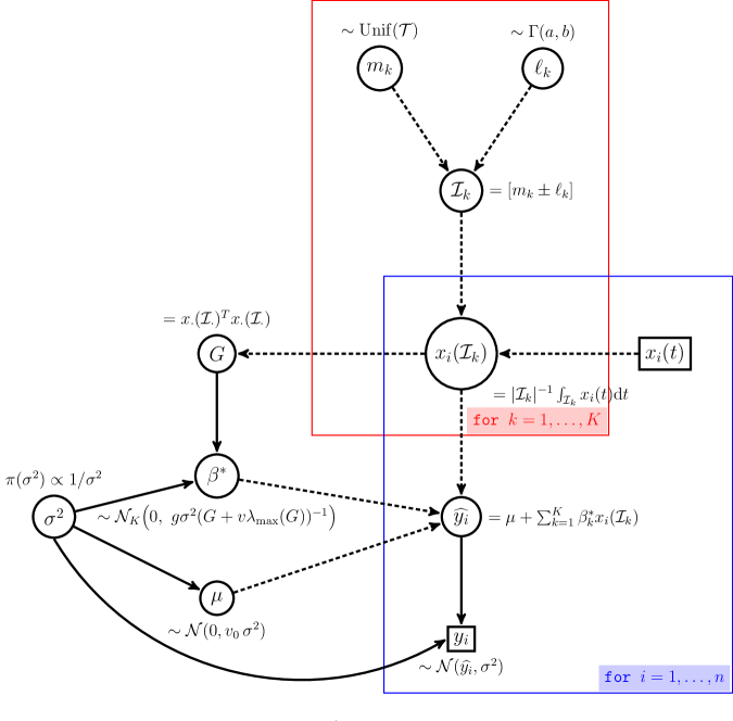
Figure 1: The full Bayesian model. The coefficient function $\beta(t)=\sum_{k=1}^{K}\beta^{\ast}_{k}\mathds{1}\{t\in\mathcal{I}_{k}\}/|\mathcal{I}_{k}|$ defines both a projection the covariate functions $x_{i}(t)$ onto $\mathbb{R}^{K}$ by averaging the function over each interval $\mathcal{I}_{k}$ and a prediction $\widehat{y_{i}}$ which depends on the vector $\beta^{\ast}=(\beta^{\ast}_{1},\ldots,\beta^{\ast}_{K})$ and the intercept $\mu$.

Given the intervals, or equivalently, given the $m_{k}$’s and $\ell_{k}$’s, the functional linear model becomes a multivariate linear model with $x_{i}(\mathcal{I}_{k})$ as scalar covariates. We could have set a standard and well-understood prior on $\beta^{\ast}|(\mathcal{I}_{k})_{1\leq k\leq K}$, namely the $g-$Zellner prior, with $g=n$ in order to define a vaguely informative prior. More specifically, the design matrix given the intervals is

$$x_{\cdot}(\mathcal{I}_{\cdot})=\left\{x_{i}(\mathcal{I}_{k}),\ 1\leq i\leq n,\ 1\leq k\leq K\right\}.$$

And the $g$-Zellner prior, with $g=n$ is given by

$$\pi(\sigma^{2})\propto 1/\sigma^{2},\quad\beta^{\ast}|\sigma^{2}\sim\mathcal{N}_{K}\bigg{(}0,n\sigma^{2}G^{-1}\bigg{)}$$ (8)

where $\beta^{*}=(\beta_{1}^{*},\dots,\beta_{K}^{*})$ and $G=x_{\cdot}(\mathcal{I}_{\cdot})^{T}x_{\cdot}(\mathcal{I}_{\cdot})$ is the Gram matrix. But, depending on the intervals $\mathcal{I}_{k}$, the covariates $x_{i}(\mathcal{I}_{k})$ can be highly correlated. (We recall here that the functional covariate can have autocorrelation and that the intervals can overlap.) That is why, in this setting, the Gram matrix $G=x_{\cdot}(\mathcal{I}_{\cdot})^{T}x_{\cdot}(\mathcal{I}_{\cdot})$ can be ill-conditioned, that is to say not numerically invertible and we cannot resort to the $g-$Zellner prior. To solve this issue we have to decrease the condition number of $G$, and apply a Tikhonov regularization. The resulting prior is a ridge-Zellner prior (Baragatti and Pommeret, , 2012) replaces $G$ by $G+\eta I$ in (8), where $\eta$ is some scalar tuning the amount of regularization and $I$ is the identity matrix. Adding the $\eta I$ matrix shifts all eigenvalues of the Gram matrix by $\eta$. In order to obtain a well-conditioned matrix, we decided to fix $\eta$ with the help of the largest eigenvalue of the Gram matrix, $\lambda_{\text{max}}(G)$ and to set $\eta=v\lambda_{\text{max}}(G)$ where $v$ is an hyperparameter of the model.

To sum up the above, the prior distribution on $\Theta_{K}$ is

$$\mu|\sigma^{2} \sim\mathcal{N}\left(0,v_{0}\sigma^{2}\right),$$

$$\beta^{*}|\sigma^{2} \sim\mathcal{N}_{K}\left(0,n\sigma^{2}(G+v\lambda_{\text{max}}(G)I)^{-1}\right),\text{ where }G=x_{\cdot}(\mathcal{I}_{\cdot})^{T}x_{\cdot}(\mathcal{I}_{\cdot}),$$

$$\pi(\sigma^{2}) \propto 1/\sigma^{2},$$ (9)

$$m_{k} \overset{i.i.d.}{\sim}\text{Unif}\left(\mathcal{T}\right),\quad k=1,\ldots,K,$$

$$\ell_{k} \overset{i.i.d.}{\sim}\Gamma(a,1),\quad k=1,\ldots,K,$$

The resulting Bayesian modelling is given in Figure 1 and depends on hyperparameters which are $v_{0},v,a$ and $K$. We denote by $\pi_{K}(\theta)$ and $\pi_{K}(\theta|\mathcal{D})$ the prior and the posterior distributions. We propose below default values for the hyperparameters $v_{0},v,a$, see Section 3.4 for numerical results that supports this proposal.

• The parameter $v_{0}$ drives the prior information we put on the intercept $\mu$. This is clearly not the most important hyperparameter since we expect important information regarding $\mu$ in the likelihood. We recommend using $v_{0}=100\times\bar{y}^{2}$, where $\bar{y}$ is the average of the outcome on the dataset. Even if it may look like we set the prior with the current data, the resulting prior is vaguely non-informative.

• The parameter $v$ is more difficult to set: it tunes the amount of regularization in the $g$-Zellner prior. Our set of numerical studies indicates, see Section 3 below, that $v=5$ is a good value.

• The parameter $a$ sets the prior length of an interval of the support. It should depend on the number $K$ of intervals. We recommend the value $a=(5K)^{-1}$ so that the average length of an interval from the prior distribution is proportional to $1/K$. Our numerical studies that constant $5$ in the above recommandation does not drastically influence the results.

Finally, the hyperparameter $K$ drives the number of intervals, thus the dimension of $\Theta_{K}$. We can put an extra prior distribution on $K$ and perform Bayesian model choice either to infer $K$ or to aggregate posteriors coming from various values of $K$. There is a ban on the use of improper prior together with Bayesian model choice (or Bayes factor) because of the Jeffrey-Lindley paradox (see, e.g. Robert, , 2007, Section 5.2). And a careful reader would notice here the improper prior on $\sigma^{2}$. But it does not prohibit the use of Bayesian choice because it is a parameter common to all models (i.e., to all values of $K$ here).

2.3 Estimation of the support

Regarding the inference of the support, an interesting quantity is the posterior probability that a given $t\in\mathcal{T}$ is in the support. It can be defined as the prior probability in (7), that is to say

$$\alpha(t|\mathcal{D})=\int_{\Theta_{K}}\mathbf{1}\{t\in S_{\theta}\}\pi_{K}(\theta|\mathcal{D})\mathrm{d}\theta.$$ (10)

Both functions $\alpha(t)$ and $\alpha(t|\mathcal{D})$ can be easily computed with a sample from the prior and the posterior respectively. They are also relatively easy to interpret in term of marginal distribution of the support: fix $t\in\mathcal{T}$,

• $\alpha(t)$ is the prior probability that $t$ is in the support of the coefficient function and

• $\alpha(t|\mathcal{D})$ is the posterior probability of the same event.

Now let $L_{\gamma}(S,S_{\theta})$ be the loss function given by

$$L_{\gamma}(S,S_{\theta})=\gamma\int_{0}^{1}\mathbf{1}\{t\in S\setminus S_{\theta}\}\mathrm{d}t+(1-\gamma)\int_{0}^{1}\mathbf{1}\{t\in S_{\theta}\setminus S\}\mathrm{d}t$$ (11)

where $S_{\theta}=\operatorname{Supp}(\beta_{\theta})$ is the support of $\beta_{\theta}(t)$, the coefficient function as parametrized in (5) and where $\gamma$ is a tuning parameter in $[0;1]$. Actually, there is two type of errors when estimating the support:

• error of type I: a point $t\in\mathcal{T}$ which is really in the support $S_{\theta}$ has not been included in the estimate,

• error of type II: a point $t\in\mathcal{T}$ has been included in the support estimate but does not lie into the real support $S_{\theta}$

and the tuning parameter $\gamma$ allows to set different weights on both types of error. Note that, when $\gamma=1/2$, the loss function is one half of the Lebesgue measure of the symmetric difference $S\Delta S_{\theta}$.

Bayes estimates are obtained by minimizing a loss function integrated with respect to the posterior distribution, see Robert, (2007). Hence, in this situation, Bayes estimates of the support are given by

$$\widehat{S}_{\gamma}(\mathcal{D})\in\underset{S\subset\mathcal{T}}{\operatorname{arg\,min}~{}}\int_{\Theta_{K}}L_{\gamma}(S,S_{\theta})\pi_{K}(\theta|\mathcal{D})\mathrm{d}\theta.$$ (12)

The following theorem shows the existence of the Bayes estimate and how to compute it from $\alpha(t|\mathcal{D})$.

Theorem 1.

The level set of $\alpha(t|\mathcal{D})$ defined by

$$\widehat{S}_{\gamma}(\mathcal{D})=\{t\in\mathcal{T}\ :\ \alpha(t|\mathcal{D})\geq\gamma\}$$

is a Bayes estimate associated to the above loss $L_{\gamma}(S,S_{\theta})$. Moreover, up to a set of null Lebesgue measure, any Bayes estimate $\widehat{S}_{\gamma}(\mathcal{D})$ that solves the optimisation problem given in (12) satisfies

$$\{t\in\mathcal{T}\ :\ \alpha(t|\mathcal{D})>\gamma\}\subset\widehat{S}_{\gamma}(\mathcal{D})\subset\{t\in\mathcal{T}\ :\ \alpha(t|\mathcal{D})\geq\gamma\}.$$

The proof of the above theorem is given in Appendix A.1. Although simple-looking, the proof requires some caution because sets should be Borelian sets. Note that, when we try to avoid completely errors of type I (resp. type II) by setting $\gamma=0$ (resp. $\gamma=1$), the support estimate is $\mathcal{T}$ (resp. $\emptyset$). Additionally Theorem 1 shows how we should interpret the posterior probability $\alpha(t|\mathcal{D})$ and that its plot may be one important output of the Bayesian analysis proposed in this paper: it measures the evidence that a given point is in the support of the coefficient function. Finally, note that the number of intervals in the support estimate $\widehat{S}_{\gamma}(\mathcal{D})$ can, and is often different from the value of $K$ (because intervals can overlap).

2.4 Estimation of the coefficient function

The Bayesian modelling given in Section 2.2 was mainly designed to estimate the support of the coefficient function. We can nevertheless provide Bayes estimates of the coefficient function. We propose here two Bayes estimates of the coefficient function. The first one, given in Equation (13) is a smooth estimate, whereas the second estimate, given in Proposition 3, is a stepwise estimate which is parsimonious and may be more easily interpreted.

With the default quadratic loss, a Bayes estimate is defined as

$$\widehat{\beta}_{L^{2}}(\cdot)\in\underset{d(\cdot)\in L^{2}(\mathcal{T})}{\operatorname{arg\,min}}\iint\left(\beta_{\theta}(t)-d(t)\right)^{2}\mathrm{d}t\ \pi_{K}(\theta|\mathcal{D})\mathrm{d}\theta$$ (13)

where $\beta_{\theta}(t)$ is the coefficient function as parametrized in (5). At least heuristically $\widehat{\beta}_{L^{2}}(\cdot)$ is the average of $\beta_{\theta}(\cdot)$ over the posterior distribution $\pi_{K}(\theta|\mathcal{D})$, though the average of functions taking values in $L^{2}(\mathcal{T})$ under some probability distribution is hard to define (using either Bochner or Pettis integrals). In this simple setting we can claim the following (see Appendix A.2 for the proof).

Proposition 2.

Let $\|\cdot\|$ be the norm of $L^{2}(\mathcal{T})$. If $\int\left\|\beta_{\theta}(\cdot)\right\|\pi_{K}(\theta|\mathcal{D})\mathrm{d}\theta<\infty,$ then the estimate defined by

$$\widehat{\beta}_{L^{2}}(t)=\int\beta_{\theta}(t)\pi_{K}(\theta|\mathcal{D})\mathrm{d}\theta,\quad\ t\in\mathcal{T},$$ (14)

is in $L^{2}(\mathcal{T})$ and solves the optimization problem (13).

Averages such as (14) belong to the closure of the convex hull of the support $\mathcal{E}_{K}$ of the posterior distribution. We can prove (see Proposition 5 in Appendix A.4) that the convex hull of $\mathcal{E}_{K}$ is the set $\mathcal{E}=\cup_{K=1}^{\infty}\mathcal{E}_{K}$ of step functions on $\mathcal{T}$, and the closure of $\mathcal{E}$ is $L^{2}(\mathcal{T})$. Hence the only guarantee we have on $\widehat{\beta}_{L^{2}}$ as defined in (14) is that $\widehat{\beta}_{L^{2}}$ lies in $L^{2}(\mathcal{T})$, a much larger space than the set of step functions. Though not shown here, integrating the $\beta_{\theta}(t)$’s over $\theta$ with respect to the posterior distribution has regularizing properties, and the Bayes estimate $\widehat{\beta}_{L^{2}}(t)$ is smooth.

To obtain an estimate lying in the set of step functions, namely $\mathcal{E}$, we can consider the projection of $\widehat{\beta}_{L^{2}}$ onto the set $\mathcal{E}_{K_{0}}$ for a suitable value of $K_{0}$ possibly different to $K$. However, due to the topological properties of $L^{2}(\mathcal{T})$ and $\mathcal{E}_{K_{0}}$, the projection of $\widehat{\beta}_{L^{2}}$ onto the set $\mathcal{E}_{K_{0}}$ does not always exist (see Appendix A.4). To address this problem, we introduce a subset $\mathcal{E}_{K_{0}}^{\varepsilon}$ of $\mathcal{E}_{K_{0}}$, where $\varepsilon>0$ is a tuning parameter. Let $\mathcal{F}^{\varepsilon}$ denote the set of step functions $\beta(t)\in L^{2}(\mathcal{T})$ which can be written as

$$\beta(t)=\sum\beta^{\dagger}_{k}\mathds{1}\{t\in J_{k}\}$$

where the intervals $J_{k}$’s are mutually disjoint and each of the lengths are greater than $\varepsilon$. The set $\mathcal{E}_{K_{0}}^{\varepsilon}$ is now defined as $\mathcal{F}^{\varepsilon}\cap\mathcal{E}_{K_{0}}$. By considering this set, we remove from $\mathcal{E}_{K}$ the step functions which have intervals of very small length, and we can prove the following.

Proposition 3.

Let $K_{0}\geq 1$ and $\varepsilon>0$.

• The function $d(\cdot)\mapsto\|d(\cdot)-\widehat{\beta}_{L^{2}}(\cdot)\|^{2}$ admits a minimum on $\mathcal{E}_{K_{0}}^{\varepsilon}$. Thus a projection of $\widehat{\beta}_{L^{2}}(\cdot)$ onto this set, defined by

  $$\widehat{\beta}_{K_{0}}^{\varepsilon}(\cdot)\in\underset{d(\cdot)\in\mathcal{E}_{K_{0}}^{\varepsilon}}{\operatorname{arg\,min}}\ \|d(\cdot)-\widehat{\beta}_{L^{2}}(\cdot)\|^{2},$$ (15)

  always exists.

• The estimate $\widehat{\beta}_{K_{0}}^{\varepsilon}(\cdot)$ is a true Bayes estimate with loss function

  $$L_{K_{0}}^{\varepsilon}\big{(}d(\cdot),\beta(\cdot)\big{)}=\begin{cases}\left\|d(\cdot)-\beta(\cdot)\right\|^{2}=\int_{\mathcal{T}}\left(\beta(t)-d(t)\right)^{2}\mathrm{d}t&\text{if }\beta\in\mathcal{E}_{K_{0}}^{\varepsilon},\\ +\infty&\text{otherwise}.\end{cases}$$ (16)

  That is to say

  $$\widehat{\beta}_{K_{0}}^{\varepsilon}(\cdot)\in\underset{d(\cdot)\in L^{2}(\mathcal{T})}{\operatorname{arg\,min}}\ \int L_{K_{0}}^{\varepsilon}\big{(}d(\cdot),\beta_{\theta}(\cdot)\big{)}\pi_{K}(\theta|\mathcal{D})\mathrm{d}\theta.$$

Finally one should note that the support of the Bliss estimate given in Proposition 3 provides another estimate of the support, which differs from the Bayes estimate introduced in Section 2.3. Obviously, real Bayes estimates, which optimizes the loss integrated over the posterior distribution, are by construction better estimates. Another possible alternative would be the definition of an estimate of the coefficient function whose support is given by one of the Bayes estimates defined in Theorem 1. But such estimates do not account for the inferential error regarding the support. Hence we believed that, when it comes to estimating the coefficient function, the Bayes estimates proposed in this Section are better than other candidates and achieve a trade off between inferential errors on its support and prediction accuracy on new data.

2.5 Implementation

The full posterior distribution can be written explicitly from the Bayesian model given in Equations (9). As usual with hierarchical models, sampling from the posterior distribution $\pi_{K}(\theta|\mathcal{D})$ can be done with a Gibbs algorithm (see, e.g., Robert and Casella, , 2013, Chapter 7). The details of the MCMC algorithm are given in Appendix B.1.

Now let $\theta(s)$, $s=1,\ldots,N$, denote the output of the MCMC sampler after the burn-in period. The computation of the Bayes estimate $\widehat{S}_{\gamma}(\mathcal{D})$ of the support as defined in Theorem 1 depends on the probabilities $\alpha(t|\mathcal{D})$. With the Monte Carlo sample from the MCMC, we can easily approximate these posterior probabilities by the frequencies

$${\alpha}(t|\mathcal{D})\approx\frac{1}{N}\sum_{s=1}^{N}\mathds{1}\{\beta_{\theta(s)}(t)\neq 0\}.$$

What remains to be computed are the approximations of $\widehat{\beta}_{L^{2}}(\cdot)$ and $\widehat{\beta}_{K_{0}}^{\varepsilon}(\cdot)$ based on the MCMC sample. First, the Monte Carlo approximation of (14) is given by

$$\widehat{\beta}_{L^{2}}(t)\approx\frac{1}{N}\sum_{s=1}^{N}\beta_{\theta(s)}(t).$$

And the more interesting Bayes estimate $\widehat{\beta}_{K_{0}}^{\varepsilon}(\cdot)$ can be computed by minimizing

$$\left\|d(\cdot)-\frac{1}{N}\sum_{s=1}^{N}\beta_{\theta(s)}(\cdot)\right\|^{2}$$

over the set $\mathcal{E}_{K_{0}}^{\varepsilon}$. To this end we run a Simulated annealing algorithm (Kirkpatrick et al., , 1983), described in Appendix B.2.

We also provide a striking graphical display of the posterior distribution on the set $\mathcal{E}_{K}$ with a heat map. More precisely, the aim is to sketch all marginal posterior distributions $\pi^{t}_{K}(\cdot|\mathcal{D})$ of $\beta_{\theta}(t)$ for any value of $t\in\mathcal{T}$ in one single figure. To this end we introduce the probability measure $Q$ on $\mathcal{T}\times\mathbb{R}$ defined as follows. Its marginal distribution over $\mathcal{T}$ is uniform, and given the value $t$ of the first coordinate, the second coordinate is distributed according to the posterior distribution of $\beta(t)$. In other words,

$$(t,b)\sim Q\quad\iff\quad t\sim\text{Unif}(\mathcal{T}),\ b|t\sim\pi^{t}_{K}(\cdot|\mathcal{D}).$$

We can easily derive an empirical approximation of $Q$ from the MCMC sample $\{\theta(s)\}$ of the posterior. Indeed, the first marginal distribution of $Q$, namely $\text{Unif}(\mathcal{T})$ can be approximated by a regular grid $t_{i}$, $i=1,\ldots,M$. And, for each value of $i$, set $b_{is}=\beta_{\theta(s)}(t_{i})$, $s=1,\ldots,N$. The resulting empirical measure is

$$\widehat{Q}=\frac{1}{M\,N}\sum_{i=1,\ldots,M}\sum_{j=1,\ldots,N}\delta_{(t_{i},b_{is})},$$

where $\delta_{(t,b)}$ is the Dirac measure at $(t,b)$. The graphical display we propose is representing $\widehat{Q}$ with a heat map on $\mathcal{T}\times\mathbb{R}$. Each small area of $\mathcal{T}\times\mathbb{R}$ is thus colored according to its $\widehat{Q}$-probability. This should be done cautiously as the marginal posterior distribution $\pi^{t}_{K}(\cdot|\mathcal{D})$ has a point mass at zero: $\pi^{t}_{K}(b=0|\mathcal{D})>0$ by construction of the prior distribution. Finally the color scale can be any monotone function of the probabilities, in particular non linear functions to handle the atom at $0$. Examples are provided in Section 3 in Figures 4 and 5.

3 Simulation study

In this section, the performance of Bliss is evaluated and compared to three competitors: FDA (Ramsay and Silverman, , 2005), Fused lasso (Tibshirani et al., , 2005) and Flirti (James et al., , 2009), using simulated datasets.

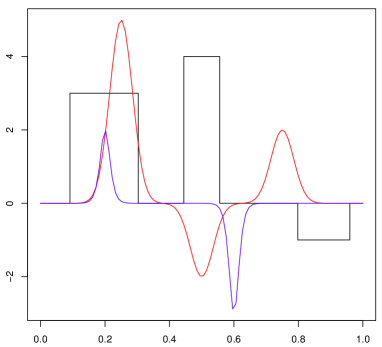
Figure 2: Coefficient functions for numerical illustrations. The black (resp. red and blue) curve corresponds to the coefficient function of Shape 1 (resp. 2 and 3).

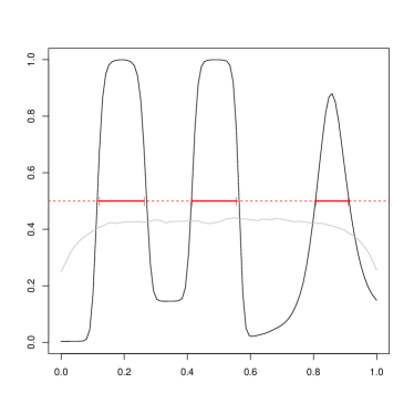
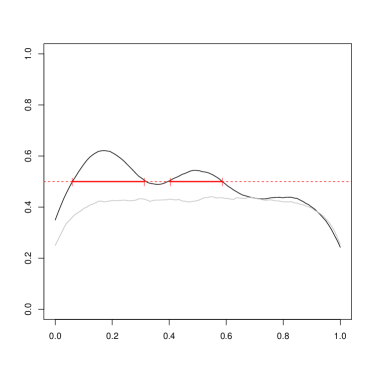
Dataset 1 ($r=5$, $\zeta=1$)	Dataset 3 ($r=5$, $\zeta=1/5$)

Figure 3: Prior (in gray) and posterior (in black) probabilities of being in the support computed on Datasets 1 and 2. Bayes estimate of support using Theorem 1 with $\gamma=1/2$ are given in red.

3.1 Simulation scheme

First of all, we describe how we generate different datasets on which we applied and compared the methods. The support of the covariate curves $x_{i}$ is $\mathcal{T}=[0,1]$, observed on a regular grid $(t_{j})_{j=1,\dots,p}$ on $\mathcal{T}$, for $p=100$. We simulate $p$-multivariate Gaussian vectors $x_{i}$, $i=1,\dots,100$, corresponding to the values of curves $x_{i}$ for the observation times $(t_{j})_{j}$. The covariance matrix $\Sigma$ of these Gaussian vectors is given by

$$\Sigma_{i,j}=\sqrt{\Sigma_{i,i}\Sigma_{j,j}}\exp\left(-\zeta^{2}(t_{i}-t_{j})^{2}\right),\hskip 14.22636pt\text{ for $i$ and $j$ from 1 to $p$},$$

where the coefficient $\zeta$ tunes the autocorrelation of the $x_{i}(t)$. Three different shapes are considered for the functional coefficient $\beta$, given in Figure 2.

The first one is a step function, the second one is smooth and is null on small intervals of $\mathcal{T}$ (Smooth), the third one is nonnull only on small intervals of $\mathcal{T}$ (Spiky).

• Step function: $\beta(t)=3\,\mathbf{1}{\{t\in[0.1,0.3]\}}+4\,\mathbf{1}\{t\in[0.45,0.55]\}-\mathbf{1}\{t\in[0.8,0.95]\}$.

• Smooth: $\beta(t)=5\times e^{-20(t-0.25)^{2}}-2\times e^{-20(t-0.5)^{2}}+2\times e^{-20(t-0.75)^{2}}$.

• Spiky: $\beta(t)=8\times\big{(}2+e^{20-100t}+e^{100t-20}\big{)}^{-1}-12\times\big{(}2+e^{60-100t}+e^{100t-60}\big{)}^{-1}$.

The outcomes $y_{i}$ are calculated according to (3) with an additional noise following a centred Gaussian distribution with variance $\sigma^{2}$. The value of $\sigma^{2}$ is fixed such that the signal to noise ratio is equal to a chosen value $r$. Datasets are simulated for $\mu=1$ and for the following different values of $\zeta$ and $r$:

• $\zeta=1,{1}/{3},{1}/{5}$,

• $r=1,3,5.$

Hence, we simulate 27 datasets with different characteristics, that we use in Section 3.3 to compare the methods.

3.2 Performances regarding support estimates

Table 1: Comparison of the support estimate and the support of the Bliss estimate.

			Support Error		Dataset
Shape	$r$	$\zeta$	Support of the stepwise estimate	Bayes support estimate
Step function	$5$	$1$	0.242	0.152	1
	$5$	$1/3$	0.384	0.202	2
	$5$	$1/5$	0.242	0.293	3
2-6	$3$	$1$	0.232	0.091	4
	$3$	$1/3$	0.323	0.394	5
	$3$	$1/5$	0.424	0.465	6
2-6	$1$	$1$	0.283	0.162	7
	$1$	$1/3$	0.404	0.333	8
	$1$	$1/5$	0.439	0.394	9
2-6

Section 3.1 describes the simulation scheme of the datasets. Section 3.3 describes the criteria: Support Error. We begin by assessing the performances of our proposal in term of support recovery. We focus here on the datasets simulated with the step function as the true coefficient function. It is the only function among the three functions we have chosen where the real definition of the support matches with the answer a statistician would expect, see Figure 1. The numerical results are given in Table 3.2, where we evaluated the error with the Lebesgue measure of the symmetric difference between the true support $S_{0}$ and the estimated one $\widehat{S}$, that is to say $2L_{1/2}(\widehat{S},S_{0})$ with the notation of Section 2.3.

As we claim at the end of Section 2.4, the Bayes estimates we have defined in Theorem 1 performs much better than relying on the support of a stepwise estimate of the coefficient function. As also expected the accuracy of the Bayes support estimate worsens when the autocorrelation within the functional covariate $x_{i}(t)$ increases. The signal to noise ratio is the second most influent factor that explains the accuracy of the estimate.

The third interval of the true support, namely $[0.8,0.95]$, is the most difficult to recover because the true value of the coefficient function over this interval is relatively low ($-1$) compared to the other values ($4$ and $3$) of the coefficient function. Figure 3 gives two examples of the posterior probability function $\alpha(t|\mathcal{D})$ defined in Eq. (10) where we have highlighted (in red) the Bayes support estimate with $\gamma=1/2$. Among these two examples, the Figure shows that the third interval is recovered only when there is low autocorrelation in $x_{i}(t)$ (i.e. Dataset 1). Figure 3 exhibits that the support estimate of Dataset 1 (low autocorrelation within the covariate) is more trustworthy than the support estimate of Dataset 3 (high autocorrelation within the covariate).

For more complex coefficient functions, see Figure 2, we cannot compare directly the Bayes support estimate with the true support of the coefficient function that generated the data. Nevertheless, in the next section, we will compare the coefficient estimate with the true value of the coefficient function.

3.3 Performances regarding the coefficient function

Flirti	Fused Lasso
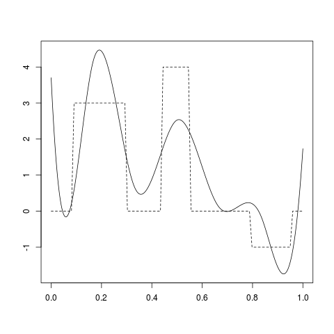
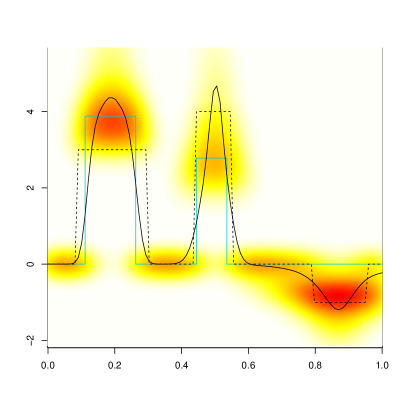
FDA	Bliss

Figure 4: Estimates of the coefficient function on Dataset 4 ($r=3$, $\zeta=1$)

Flirti	Fused Lasso
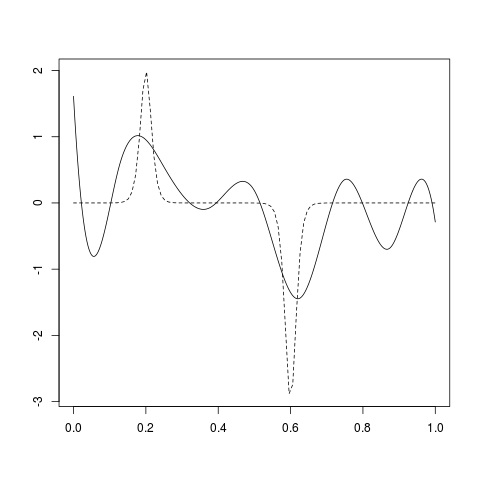
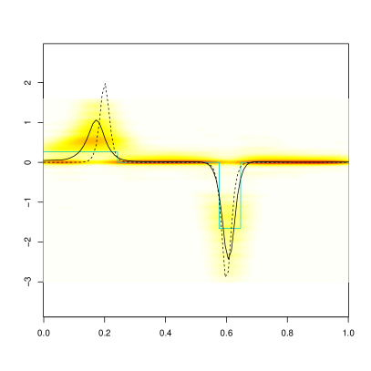
FDA	Bliss

Figure 5: Estimates of the coefficient function on Dataset 25 ($r=1$, $\zeta=1$))

In order to compare the methods for the estimation of the coefficient function, we use the $L^{2}$-loss, namely

$$\int_{0}^{1}(\widehat{\beta}(t)-\beta_{0}(t))^{2}\mathrm{d}t$$

where $\widehat{\beta}(t)$ is an estimate we compare to the true coefficient function $\beta_{0}(t)$. Table LABEL:tab:estimate_error shows the results of Bliss and its competitors on these simulated datasets. It appears that the numerical results of the three methods have the same order of magnitude. Although the three methods may have different accuracy, depending on the shape of the coefficient function that generated the dataset.

Regarding Fused Lasso, we can see in Table LABEL:tab:estimate_error that its accuracy worsens when the problem is not sparse, that is to say when the true function is the “smooth” function (the red curve of Figure 2). Next, we observe that Flirti is very sensitive. Its numerical results can be sometimes rather accurate, but sometimes the $L^{2}$-error can blow up (to exceed $100$) because the method did not manage to tune its parameters. The $L^{2}$-Bliss estimate defined in Proposition 2 frequently overperforms the other methods. This first conclusion is not surprising because the $L^{2}$-Bliss estimate has been defined to optimize the $L^{2}$-loss integrated over the posterior distribution.

Even in situations where the true function is stepwise, the stepwise Bliss estimate of Proposition 3 is less accurate than the $L^{2}$-Bliss estimate, except for two examples (datasets 6 and 9). Nevertheless we do argue that the stepwise Bliss estimate was built to provide a trade off between accuracy regarding the support estimate and accuracy regarding the coefficient function estimate. Thus the stepwise estimate is a balance between support estimate and coefficient function estimate that can help the statistician who can then get an interpretation of the underlying phenomena that generated the data. In other words, the stepwise-Bliss estimate is not the best neither at estimating the support nor at approximating the coefficient function, but provides a tradeoff.

To show more detailed results we have presented the estimate of the coefficient function in two cases.

• Figure 4 displays the numerical results on Dataset 4 (medium level of signal, low level of autocorrelation with the covariates). As can be expected when the true coefficient is a stepwise function, the stepwise Bliss estimate behaves nicely. The representation of the marginals of the posterior distribution with a heat map shows the confidence we can have in the Bayes estimate of the coefficient function. The smooth estimate nicely follows the regions of high posterior density. Here, the stepwise estimate clearly highlights two time periods (the first two intervals of the true support) and the sign of the coefficient function on these intervals. We can compare our proposal with its competitors. Flirti did not manage to tune its own parameters, and the Flirti estimate is completely irrelevant. Fused Lasso on a discretized version of the functional covariate provides a relatively nice estimate of the coefficient function. And FDA is not that bad, although the estimate is clearly too smooth to match the true coefficient function.

• Figure 5 displays the numerical results on Dataset 25 (low level of signal, and low level of autocorrelation within the covariates). In this example, the true coefficient is not stepwise, but smooth, and is around zero on large time periods. The $L^{2}$-Bliss estimate of Proposition 2 matches approximately the true coefficient function. The stepwise-Bliss estimate is a little bit poorer (maybe because of the difficult calibration of the simulated annealing algorithm). When comparing these results with other estimates on this dataset, we see that Flirti and Fused Lasso performed also decently, even if they both highlight a third time period (around $t=0.85$) where they infer a negative coefficient function instead of $0$. Flirti is at its best here, and has obviously managed to tune its own parameters in a relevant way. The confidence bands of Flirti are then reliable, but we stress here that they are relatively wide around periods where the Flirti estimate is null and does not reflect high confidence in any support estimate based on Flirti. Finally, the comments on FDA are the same as Dataset 4, the FDA estimate is clearly too smoothed to match the true coefficient function.

Table 2: Numerical results of Bliss, Flirti, Fused lasso and FDA on the Simulated Datasets.

			$L^{2}$-error					Dataset
Shape	$r$	$\zeta$	stepwise Bliss	$L^{2}$-Bliss	Fused lasso	Flirti	FDA
Step function	$5$	$1$	1.126	0.740	0.666	1.288	1.514	1
	$5$	$1/3$	2.221	1.415	1.947	1.781	1.997	2
	$5$	$1/5$	2.585	1.656	1.777	3.848	1.739	3
2-9	$3$	$1$	1.283	0.821	0.984	$10^{3}$	1.203	4
	$3$	$1/3$	1.531	1.331	1.936	$10^{4}$	1.830	5
	$3$	$1/5$	2.266	2.989	2.036	1.772	2.144	6
2-9	$1$	$1$	1.589	0.747	0.995	3.848	1.577	7
	$1$	$1/3$	2.229	1.817	2.214	$10^{4}$	2.307	8
	$1$	$1/5$	1.945	2.364	2.028	3.848	4.437	9
2-9 Smooth	$5$	$1$	0.510	0.134	0.601	0.166	0.573	10
	$5$	$1/3$	0.807	0.609	0.442	2.068	1.103	11
	$5$	$1/5$	1.484	1.352	2.325	2.068	1.650	12
2-9	$3$	$1$	0.776	0.416	0.320	0.263	3.295	13
	$3$	$1/3$	0.855	0.954	6.790	2.068	1.819	14
	$3$	$1/5$	1.291	1.162	1.742	1.328	1.759	15
2-9	$1$	$1$	0.932	0.641	0.652	2.335	0.616	16
	$1$	$1/3$	0.719	0.283	0.613	$10^{4}$	1.308	17
	$1$	$1/5$	1.536	1.006	4.680	5.430	2.985	18
2-9 Spiky	$5$	$1$	0.099	0.013	0.059	0.035	0.239	19
	$5$	$1/3$	0.208	0.144	0.260	0.271	0.349	20
	$5$	$1/5$	0.285	0.251	0.181	0.226	0.306	21
2-9	$3$	$1$	0.187	0.023	0.638	0.136	0.584	22
	$3$	$1/3$	0.257	0.202	0.159	0.277	0.258	23
	$3$	$1/5$	0.269	0.260	0.459	0.276	1.050	24
2-9	$1$	$1$	0.144	0.087	0.123	0.166	0.270	25
	$1$	$1/3$	0.242	0.223	0.260	$10^{2}$	0.270	26
	$1$	$1/5$	0.273	0.279	0.221	0.301	0.405	27
2-9

3.4 Tuning the hyperparameters

We can now discuss our recommandation on the hyperparameters of the model, given at the end of Section 2.2. For this study, we applied our methodology on Dataset 1 and fixed the hyperparameters $v_{0}$, $v$, $a$ around the recommended values.We recall that Dataset 1 is a synthetic dataset simulated with a coefficient function that is a step function (the black curve of Figure 2), with a high level of signal over noise ($r=5$) and with a low level of autocorrelation within the covariates($\zeta=1$). The following values are considered for each hyperparameter:

• for $a$: $0.5/K$, $0.2/K$, $0.1/K$, $0.07/K$ and $0.05/K$;

• for $v$: 10, 5, 2, 1 and 0.5;

• and for $K$: any integer between $1$ and $10$.

The numerical results are given in Table 3.4. The default values we recommend are not the best values here, but we have done numerous other trials on many synthetic datasets and these choices are relatively robust. We do not highlight any particular value for $K$ since this value can (and should) be chosen with the Bayesian model choice machinery.

Table 3: Performances of Bliss with respect to the tuning of the hyperparameters.

The $\heartsuit$ symbol indicates the default values.

4 Application to the black Périgord truffle dataset

We apply the Bliss method on a dataset to predict the amount of production of black truffles given the rainfall curves.

Figure 6: Rainfall of the Truffle datsaset. Left:Plot shows the rainfall for each year, color-coded by their truffle yield. Right:Autocorrelation of the 13 observed rainfall covariates, with lag in number of ten-day periods.

The black Périgord truffle (Tuber Melanosporum Vitt.) is one of the most famous and valuable edible mushrooms, because of its excellent aromatic and gustatory qualities. It is the fruiting body of a hypogeous Ascomycete fungus, which grows in ectomycorrhizal symbiosis with oaks species or hazelnut trees in Mediterranean conditions. Modern truffle cultivation involves the plantation of orchards with tree seedlings inoculated with Tuber Melanosporum. The planted orchards could then be viewed as ecosystems that should be managed in order to favour the formation and the growth of truffles. The formation begins in late winter with the germination of haploid spores released by mature ascocarps. Tree roots are then colonised by haploid mycelium to form ectomycorrhizal symbiotic associations. Induction of the fructification (sexual reproduction) occurs in May or June (the smallest truffles have been observed in mid-June). Then the young truffles grow during summer months and are mature between the middle of November and the middle of March (harvest season). The production of truffles should then be sensitive to climatic conditions throughout the entire year (Le Tacon et al., , 2014). However, to our knowledge few studies focus on the influence of rainfall or irrigation during the entire year (Demerson and Demerson, , 2014; Le Tacon et al., , 2014). Our aim is then to investigate the influence of rainfall throughout the entire year on the production of black truffles. Knowing this influence could lead to a better management of the orchards, to a better understanding of the sexual reproduction, and to a better understanding of the effects of climate change. Indeed, concerning sexual reproduction, Le Tacon et al., (2014, 2016) made the assumption that climatic conditions could be critical for the initiation of sexual reproduction throughout the development of the mitospores expected to occur in late winter or spring. And concerning climate change, its consequences on the geographic distribution of truffles is of interest (see Splivallo et al., , 2012 or Büntgen et al., , 2011, among others).

The analyzed data were provided by J. Demerson. They consist of the rainfall records on an orchard near Uzès (France) between 1985 and 1999, and of the production of black truffles on this orchard between 1985 and 1999. In practice, to explain the production of the year $n$, we take into account the rainfall between the 1st of January of the year $n-1$ and the 31st of March of the year $n$. Indeed, we want to take into account the whole life cycle, from the formation of new ectomycorrhizas following acospore germination during the winter preceding the harvest (year $n-1$) to the harvest of the year $n$. The cumulative rainfall is measured every 10 days, hence between the 1st of January of the year $n-1$ and the 31st of March of the year $n$ we have the rainfalls associated with 45 ten-day periods, see Figure 3.2. This dataset can be considered as reliable, as the rainfall records have been made exactly on the orchard, and the orchard was not irrigated.

Biological assumptions at stake

From the literature we can spotlight the following periods of time which might influence the growth of truffles.

• Late spring and summer of year $n-1$. This is the (only) period for which all experts are unanimous to say it has a particular effect. Büntgen et al., (2012), Demerson and Demerson, (2014) or Le Tacon et al., (2014) all confirm the importance of the negative effect of summer hydric deficit on truffle production: they found it to be the most important factor influencing the production. Indeed, in summer the truffles need water to survive the high temperatures and to grow. Otherwise they can dry out and die.

• Late winter of year $n-1$, as shown by Demerson and Demerson, (2014) and Le Tacon et al., (2014). Indeed, as explained in Le Tacon et al., (2014), consistent water availability in late winter could support the formation of new mycorrhizae, thus allowing a new cycle. Moreover, from results obtained by Healy et al., (2013) they made the assumption that rainfall is critical for the initiation of sexual reproduction throughout development of mitospores, which is expected to occur in late winter or spring of the year $n-1$. This is an assumption as the occurrence and the initiation of sexual reproduction is largely unknown, see Murat et al., (2013) or Le Tacon et al., (2016).

• November and December of year $n-1$, as claimed by Demerson and Demerson, (2014) and Le Tacon et al., (2014). Le Tacon et al. explained that rainfall in autumn allows the growth of young truffles which have survived the summer.

• September of year $n-1$, as claimed by Demerson and Demerson, (2014). Excess water in this period should be harmuful to truffles. The assumption made was that in September the soil temperature is still high, so micro-organisms responsible for rot are quite active, while a wet truffle has its respiratory system disturbed and can not defend itself against these micro-organisms.

The challenge is to confirm some of these periods with Bliss, despite the small size of the dataset. In particular, each rainfall curve is discretized with only 45 points (cumulative rainfall every 10 days) and we have at our disposal only 13 observations.

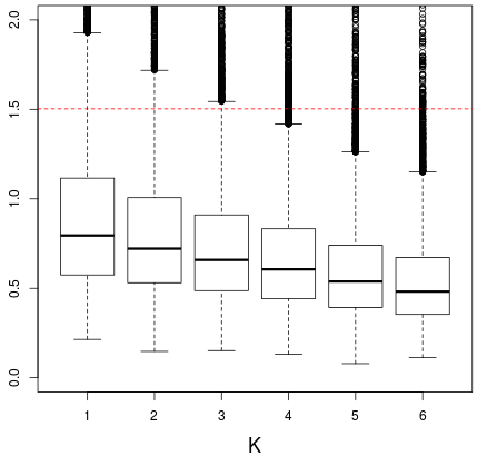
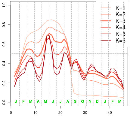
Figure 7: Sensitivity of Bliss to the value of $K$ on the truffle dataset. Left: Boxplot of the posterior distribution of the variance of the error, $\sigma^{2}$, compared to the variance of the output $y$ (red dashed line). Right: Posterior probability $\alpha(t|\mathcal{D})$ for different values of $K$.

Running Bliss

As explained above (in Section 3.2), part of the difficulty of the inference problem comes from autocorrelation within the covariate. Figure 3.2 shows that the autocorrelation can be considered as null when the lag is 3 or more in number of ten-day periods. In other words the rainfall background presents autocorrelation within a period of time of about a month (keeping in mind that the whole history we consider lasts 15 months).

The first and maybe most important hyperparameter is $K$, the number of intervals in the coefficient functions from the prior. Because of the discretization of the rainfall, and the number of observations, the value of $K$ should stay small to remain parsimonious. Because of the size of the dataset, we have set the hyperparameter $a$ to obtain a prior probability of being in the support of about $0.5$. The results are given in Figure 7. As can be seen on the left of this Figure, the error variance $\sigma^{2}$ decreases when $K$ increases, because models of higher dimension can more easily fit the data. The main question is when do they overfit the data? Looking at the right panel of Figure 7, we can consider how the posterior probability $\alpha(t|\mathcal{D})$ depends on the value of $K$ and choose a reasonable value. First, for $K=1$ or $2$, the posterior probability is high during a first long period time until August of year $n-1$ and falls to much lower values after that. Thus, these small values of $K$ provide a rough picture of dependency. Secondly, for $K=4,5$ or $6$, the posterior probability $\alpha(t|\mathcal{D})$ varies between $0.2$ and $0.7$ and shows doubtful variations after November of year $n-1$ and other strong variations during the summer of year $n-1$ that are also doubtful. Hence we decided to rely on $K=3$ although this choice is rather subjective.

Conclusions on the truffle dataset

We begin by noting that about half of the variance of the output (the amount of production of truffle) is explained by the rainfall given the posterior distribution of $\sigma^{2}$ in the left panel of Figure 7. The support estimate $\widehat{S}_{0.5}(\mathcal{D})$ with $K=3$ is composed of two disjoint intervals: a first one from May of year $n-1$ to the second ten-day period of August with the highest posterior probability, and a second one from the third ten-day period of February of year $n-1$ to the end of March of year $n-1$ with a smaller posterior probability. Thus, as far as we can tell from this analysis, Periods #1 and #2 are validated by the data. Period #3 cannot be validated although the posterior probability $\alpha(t|\mathcal{D})$ presents small bumps around theses periods of time for highest values of $K$. For $K=3$, the value of $\alpha(t|\mathcal{D})$ stays around $0.3$ on Period #3. Finally, regarding Period #4, we can see a small bump on the curve $\alpha(t|\mathcal{D})$ around this period of time even for $K=3$, but the highest value of the posterior probability on this period is about $0.4$. Hence we chose to remain undecided on Period #4.

5 Conclusion

In this paper, we have provided a full Bayesian methodology to analyse linear models with time-dependent functional covariates. The main purpose of our study was to estimate of the support of the coefficient function to search the periods of time which influences the most the outcome. We rely on piecewise constant coefficient functions to set the prior, which has four benefits. The first benefit is parsimony of the Bliss model, which turns two thirds of the parameter’s dimension to the estimation of the support. The second benefit with our Bayesian setting that begins by defining the support is that we can rely on the ridge-Zellner prior to handle the autocorrelation within the functional covariate. This fact sets Bliss apart from Bayesian methods relying on spike-and-slab prior to handle sparsity. The third benefit is avoiding cross-validation to tune internal parameters of the method. Indeed, cross-validation methods optimize the performance regarding the model’s predictive power, and not the accuracy of the support estimate. And, last but not least, the fourth benefit is the ability to compute numerically the posterior probability that a given date is in the support, $\alpha(t|\mathcal{D})$, whose value gives a clear hint on the reliability of the support estimate. Nevertheless a serious limitation of our Bayesian model is that it can handle only covariate functions of one variable (we call time in the paper). Indeed the shape of the support of a function of more than one variable is much more complex than an union of intervals and cannot be easily modelled in a nonparametric, but parsimonious manner.

We have provided numerical results regarding the power of Bliss on a bunch of synthetic datasets as well as a dataset studying the black Périgord truffle. We have shown by presenting some of these examples in details how we can interpret the results of Bliss, in particular how we can rely on the posterior probabilities $\alpha(t|\mathcal{D})$ or the heatmap of posterior distribution of the coefficient function to assess the reliability of our estimates. Bliss provides two main outputs: first an estimate of the support of the coefficient function without targeting the coefficient function, and second a trade-off between support estimate and coefficient function estimate through the stepwise estimate of Proposition 3. Moreover our prior can straightforwardly be encompassed into a linear model with other functional or scalar covariates.

Acknowledgement

We are very grateful to Jean Demerson for providing the truffle dataset and for his explanations. Pierre Pudlo carried out this work in the framework of the Labex Archimède (ANR-11-LABX-0033) and of the A*MIDEX project (ANR-11-IDEX-0001-02), funded by the “Investissements d’Avenir” French Government program managed by the French National Research Agency (ANR).

Supplementary Materials

The implementation of the method is available at the following webpage: http://www.math.univ-montp2.fr/~grollemund/Implementation/BLiSS/.

Appendix A Theoretical results

A.1 Proof of Theorem 1

Without loss of generality we can assume that $\mathcal{T}=[0;1]$. We begin the proof with the following lemma whose simple proof is left to the reader.

Lemma 4.

Set $\psi^{\ast}(\gamma,\alpha)=\min\{\gamma(1-\alpha)\,;\,(1-\gamma)\alpha\}$ for any $\alpha,\gamma\in[0;1]$. We have

$$\psi^{\ast}(\gamma,\alpha)=\begin{cases}\gamma(1-\alpha)&\text{if }\gamma\leq\alpha,\\ (1-\gamma)\alpha&\text{if }\gamma\geq\alpha.\end{cases}$$

Recall that the posterior loss we optimise is given in (12), where $S$ is any Borel subset of $\mathcal{T}=[0;1]$. Using Fubini’s theorem (for non-negative functions) and the definition of $\alpha(t|\mathcal{D})$ given in (10), we have

$$\int_{\Theta_{K}}L_{\gamma}(S,S_{\theta})\pi_{K}(\theta|\mathcal{D})\mathrm{d}\theta =\gamma\int_{0}^{1}\int_{\Theta_{K}}\mathds{1}\{t\in S\setminus S_{\theta}\}\pi_{K}(\theta|\mathcal{D})\mathrm{d}\theta\mathrm{d}t$$

$$\quad+(1-\gamma)\int_{0}^{1}\int_{\Theta_{K}}\mathds{1}\{t\in S_{\theta}\setminus S\}\pi_{K}(\theta|\mathcal{D})\mathrm{d}\theta\mathrm{d}t$$

$$=\int_{0}^{1}\psi_{S}\big{(}t,\gamma,\alpha(t|\mathcal{D})\big{)}\mathrm{d}t$$ (17)

where, for all $\alpha\in[0;1]$ we have set

$$\psi_{S}(t,\gamma,\alpha)=\mathds{1}\{t\in S\}\gamma\big{(}1-\alpha\big{)}+\mathds{1}\{t\not\in S\}(1-\gamma)\alpha.$$

Now, whatever the set $S$, $\psi_{S}(t,\gamma,\alpha)\geq\psi^{\ast}(\gamma,\alpha)$. Reporting this bound in (17) yields

$$\int_{\Theta_{K}}L_{\gamma}(S,S_{\theta})\pi_{K}(\theta|\mathcal{D})\mathrm{d}\theta\geq\int_{0}^{1}\psi^{\ast}\big{(}\gamma,\alpha(t|\mathcal{D})\big{)}\mathrm{d}t$$

whatever the Borel set $S$. Moreover, this inequality is an equality if and only if the Borel set $S$ is chosen so that, for almost all $t\in[0;1]$, $\psi_{S}\big{(}t,\gamma,\alpha(t|\mathcal{D})\big{)}=\psi^{\ast}\big{(}\gamma,\alpha(t|\mathcal{D})\big{)}$. Using Lemma 4, the last condition is equivalent to saying that for almost all $t\in[0;1]$, either $\alpha(t|\mathcal{D})=\gamma$ or $\big{(}t\in S\iff\gamma\leq\alpha(t|\mathcal{D})\big{)}$. This concludes the proof of Theorem 1. ∎

A.2 Proof of Proposition 2

Obviously, $\widehat{\beta}_{L^{2}}(\cdot)$ minimizes

$$\int\int_{\mathcal{T}}\left(\beta_{\theta}(t)-d(t)\right)^{2}\mathrm{d}t\ \pi_{K}(\theta|\mathcal{D})\mathrm{d}\theta=\int_{\mathcal{T}}\int\left(\beta_{\theta}(t)-d(t)\right)^{2}\pi_{K}(\theta|\mathcal{D})\mathrm{d}\theta\ \mathrm{d}t$$

because it does optimize $\int\left(\beta_{\theta}(t)-d(t)\right)^{2}\pi_{K}(\theta|\mathcal{D})\mathrm{d}\theta$ for all $t\in\mathcal{T}$. It remains to show that $\widehat{\beta}_{L^{2}}(\cdot)\in L^{2}(\mathcal{T})$. We have

$$\|\widehat{\beta}_{L^{2}}(\cdot)\|^{2} =\int_{\mathcal{T}}\left(\int\beta_{\theta}(t)\pi_{K}(\theta|\mathcal{D})\mathrm{d}\theta\right)^{2}\mathrm{d}t$$

$$=\int_{\mathcal{T}}\iint\beta_{\theta}(t)\beta_{\theta^{\prime}}(t)\ \pi_{K}(\theta|\mathcal{D})\pi_{K}(\theta^{\prime}|\mathcal{D})\mathrm{d}\theta\mathrm{d}\theta^{\prime}\mathrm{d}t$$

$$=\iint\int_{\mathcal{T}}\beta_{\theta}(t)\beta_{\theta^{\prime}}(t)\mathrm{d}t\ \pi_{K}(\theta|\mathcal{D})\pi_{K}(\theta^{\prime}|\mathcal{D})\mathrm{d}\theta\mathrm{d}\theta^{\prime}$$

$$\leq\iint\|\beta_{\theta}(\cdot)\|\|\beta_{\theta^{\prime}}(\cdot)\|\ \pi_{K}(\theta|\mathcal{D})\pi_{K}(\theta^{\prime}|\mathcal{D})\mathrm{d}\theta\mathrm{d}\theta^{\prime}\quad\text{with Cauchy-Schwarz inequality}$$

$$\leq\left(\int\|\beta_{\theta}(\cdot)\|\pi_{K}(\theta|\mathcal{D})\mathrm{d}\theta\right)^{2}$$

And the last integral is finite because of the assumption. Hence $\widehat{\beta}_{L^{2}}(\cdot)$ is in $L^{2}(\mathcal{T})$. ∎

A.3 Proof of Proposition 3

First, the norm $\|d(\cdot)-\widehat{\beta}_{L^{2}}(\cdot)\|$ is non negative, hence the set

$$\Big{\{}\|d(\cdot)-\widehat{\beta}_{L^{2}}(\cdot)\|,\ d(\cdot)\in\mathcal{E}_{K_{0}}^{\varepsilon}\Big{\}}$$

admits an infimum. Let $m$ denote this infimum. We have to prove that $m$ is actually a minimum of the above set, namely that there exists a function $d(\cdot)\in\mathcal{E}_{K_{0}}^{\varepsilon}$ such that $m=\|d(\cdot)-\widehat{\beta}_{L^{2}}(\cdot)\|$.

To this end, we introduce a minimizing sequence $\{d_{n}(\cdot)\}$ and we will show that one of its subsequence admits a limit within $\mathcal{E}_{K_{0}}^{\varepsilon}$. Let $d_{n}(\cdot)$ be such that

$$m=\inf\Big{\{}\|d(\cdot)-\widehat{\beta}_{L^{2}}(\cdot)\|,\ d(\cdot)\in\mathcal{E}_{K_{0}}^{\varepsilon}\Big{\}}\leq\|d_{n}(\cdot)-\widehat{\beta}_{L^{2}}(\cdot)\|\leq m+2^{-n}.$$ (18)

The step function $d_{n}(\cdot)$ can be written as

$$d_{n}(t)=\sum_{k=1}^{L}\alpha_{k,n}\mathds{1}\{t\in(a_{k,n},\ b_{k,n})\}$$

where the $(a_{k,n},\ b_{k,n})$, $k=1,\ldots,L$ are non overlapping intervals. Note that their number $L$ does not depend on $n$ because all $d_{n}(\cdot)$ lie in $\mathcal{E}_{K_{0}}$ for some fixed value of $K_{0}$, and we can always choose $L=2K_{0}-1$. Moreover, because $d_{n}(t)$ is in $\mathcal{F}^{\varepsilon}$, we can assume that

$$b_{k,n}-a_{k,n}\geq\varepsilon,\quad\text{for all }k,n.$$ (19)

Now the sequence $\{a_{1,n}\}_{n}$ has its elements in the compact interval $\mathcal{T}$ hence we extract a subsequence (still denoted $\{a_{1,n}\}_{n}$) which converges an element $a_{1,\infty}$ of $\mathcal{T}$. Likewise, by extracting subsequences $2L$ times, we can assume that all sequences $\{a_{1,n}\}_{n}$,…, $\{a_{L,n}\}_{n}$, $\{b_{1,n}\}_{n}$, …, $\{b_{L,n}\}_{n}$ are convergent, and that

$$a_{k,\infty}=\lim_{n\to\infty}a_{k,n},\quad b_{k,\infty}=\lim_{n\to\infty}b_{k,n},\quad\text{and}\quad b_{k,\infty}-a_{k,\infty}\geq\varepsilon,\quad k=1,\ldots,L$$

where the last inequalities come from (19).

The sequence $d_{n}(\cdot)$ is bounded (in $L^{2}$-norm):

$$\|d_{n}(\cdot)\|\leq\|\widehat{\beta}_{L^{2}}(\cdot)\|+\|d_{n}(\cdot)-\widehat{\beta}_{L^{2}}(\cdot)\|\leq R+\sqrt{m+1}$$

with (18), where $R=\|\widehat{\beta}_{L^{2}}(\cdot)\|$. Moreover

$$\|d_{n}(\cdot)\|^{2}=\sum_{k=1}^{L}\alpha^{2}_{k,n}\big{(}b_{k,n}-a_{k,n}\big{)}\geq\varepsilon\sum_{k=1}^{L}\alpha^{2}_{k,n}.$$

Hence, each sequence $\{\alpha_{1,n}\}_{n}$, …, $\{\alpha_{L,n}\}_{n}$ is bounded. Thus, by further extracting subsubsequences, we can assume that, for $k=1,\ldots,L$,

$$\lim_{n\to\infty}\alpha_{k,n}=\alpha_{k,\infty}$$

Finally, by setting

$$d_{\infty}(\cdot)=\sum_{k=1}^{L}\alpha_{k,\infty}\mathds{1}\{t\in(a_{k,\infty},\ b_{k,\infty})\}$$

we can easily prove that $d_{n}(\cdot)$ tends to $d_{\infty}(\cdot)$ in $L^{2}$-norm and that $d_{\infty}(\cdot)\in\mathcal{E}_{K_{0}}^{\varepsilon}$. And, with (18)

$$m=\|d_{\infty}(\cdot)-\widehat{\beta}_{L^{2}}(\cdot)\|$$

which concludes the proof. ∎

A.4 Topological properties of $\mathcal{E}_{K}$

Proposition 5.

Let $K\geq 1$.

• The convex hull of $\mathcal{E}_{K}$ is $\mathcal{E}$.

• Under the $L^{2}(\mathcal{T})$-topology, the closure of $\mathcal{E}$ is $L^{2}(\mathcal{T})$.

Proof.

The result of (ii) is rather classical, see, e.g., Rudin, (1986). The convex hull of $\mathcal{E}_{K}$ includes any step function. Indeed, any step function can be written as a convex combination of simple $a\mathbf{1}\{t\in I\}$’s which all belongs to $\mathcal{E}_{K}$. Moreover, $\mathcal{E}$ is convex because it is a linear space. Hence claim (i) is proven. ∎

For a given $K$, the set of functions $\mathcal{E}_{K}$ is not suitable to define a projection of $\hat{\beta}_{L^{2}}(\cdot)$. Indeed, let $\{d_{n}(\cdot)\}$ be a minimizing sequence of the set $\big{\{}\|d(\cdot)-\hat{\beta}_{L^{2}}(\cdot)\|,\,d(\cdot)\in\mathcal{E}_{K}(\cdot)\big{\}}$, so

$$m=\inf\Big{\{}\|d(\cdot)-\widehat{\beta}_{L^{2}}(\cdot)\|,\ d(\cdot)\in\mathcal{E}_{K}\Big{\}}\leq\|d_{n}(\cdot)-\widehat{\beta}_{L^{2}}(\cdot)\|\leq m+2^{-n}.$$

Knowing that $\hat{\beta}_{L^{2}}(\cdot)$ and $d_{n}(\cdot)$ belong to $L^{2}$ for all $n$, we have d_n(.) ∈E_K ∩B_L^2(R + m +1),   for all n, where $\mathcal{B}_{L^{2}}(r)$ is the $L^{2}$-ball of radius $r$ around the origin. Note that $\mathcal{E}_{K}\cap\mathcal{B}_{L^{2}}(R+m+1)$ is not a compact set, for example consider $d_{n}(t)=\sqrt{n}\,\mathbf{1}\{t\in[0,\frac{1}{n}]\}$. Hence it is not possible to extract a subsequence of $\{d_{n}(\cdot)\}$ which converges to a $d_{\infty}(\cdot)\in\mathcal{E}_{K}$ such that $\|d(\cdot)-\hat{\beta}_{L^{2}}(\cdot)\|=m$.

Appendix B Details of the implementations

B.1 Gibbs algorithm and Full conditional distributions

The full conditional distributions for the Gibbs Sampler in Section 2.5 are the following,

$$\mu,\beta^{*}|y,\sigma^{2},m,\ell \sim\mathcal{N}_{K+1}\left((\underline{x}^{T}\underline{x}+\underline{V})^{-1}\underline{x}y~{},~{}\sigma^{2}(\underline{x}^{T}\underline{x}+\underline{V})^{-1}\right),$$

$$\sigma^{2}|y,\mu,\beta^{*},m,\ell \sim\Gamma^{-1}\left(a+\frac{n+K+1}{2},b+\frac{1}{2}\text{SSE}+\frac{1}{2}\left\|\beta^{*}-\eta\right\|^{2}_{V^{-1}}\right),$$

$$\pi\left(m_{k}|y,\mu,\beta^{*},\sigma^{2},m_{-k},\ell\right) \propto\exp\left(-{\text{SSE}}/{2\sigma^{2}}\right)\times\pi(\beta^{\ast}|m,\ell,\sigma^{2})$$

$$\pi\left(\ell_{k}|y,\mu,\beta^{*},\sigma^{2},m,\ell_{-k}\right) \propto\exp\left(-{\text{SSE}}/{2\sigma^{2}}\right)\times\pi(\ell_{k})\times\pi(\beta^{\ast}|m,\ell,\sigma^{2})$$

where $\text{SSE}=\left\|y-\mu\mathbf{1}_{n}-x_{.}(\mathcal{I}_{.})\beta^{*}\right\|^{2}$, $\underline{x}=\Big{(}\mathbf{1}_{n}~{}\mid~{}x.(\mathcal{I}.)\Big{)}$, and V = (v0-10 0 n-1(x.(I.)Tx.(I.) + v IK) ). The full conditional distributions for the hyperparameters $m_{k}$ and $\ell_{k}$ are unusual distributions. As the covariate curves $x_{i}$ are observed on a grid $\mathcal{T}_{G}=(t_{j})_{j=1,\dots,p}$, we consider that $m_{k}$ belongs to $\mathcal{T}_{G}$ and $\ell_{k}$ is such that $m_{k}\pm\ell_{k}\in\mathcal{T}_{G}$. Thus, the number of possible values for $m_{k}$ and $\ell_{k}$ is finite and the full conditional distributions of $m_{k}$ and $\ell_{k}$ are easily computable.

B.2 Simulated annealing algorithm

We give in this section the details of the Simulated Annealing algorithm we use. Let $\tilde{\Theta}_{K_{0}}=\bigotimes_{K=1}^{K_{0}}\big{(}K,\Theta_{K}\big{)}$ where $\Theta_{K}$ is the space of all $\theta=(\beta_{1}^{*},\dots,\beta_{K}^{*},m_{1},\dots,m_{K},\ell_{1},\dots,\ell_{K})$ and let the function $C(d(\cdot))=\big{\|}d(\cdot)-\hat{\beta}_{L^{2}}(\cdot)\big{\|}^{2}$.

Algorithm : Simulated Annealing

• Initialize: a deterministic decreasing schedule of temperature $(\tau_{i})_{i=1,\dots,N_{\text{SANN}}}$, a value of $K_{0}$ and an initial vector $(K_{(0)},\theta_{(0)})\in\tilde{\Theta}_{K_{0}}$.

• Compute the function $\beta_{(0)}(t)$ from $(K_{(0)},\theta_{(0)})$.

• Repeat for $i$ from $1$ to $N_{\text{SANN}}$ :

else $(K_{(i)},\theta_{(i)})=(K_{(i-1)},\theta_{(i-1)})$ (move rejected). $\bullet$ Compute the function $\beta_{(i)}(t)$ from $(K_{(i)},\theta_{(i)})$. $\bullet$ Return the iteration $(K_{(i)},\theta_{(i)})$ minimizing the criteria $C(.)$. For the schedule of temperature, we use by default a logarithmic schedule (see Bélisle, , 1992), which is given for each iteration $i$ by $$\text{Te}/\log\left((i-1)+e\right),$$ (20) where Te is a parameter to calibrate and corresponds to the initial temperature. The result of the Simulated Annealing algorithm is sensitive to the scale of Te and it is quite difficult to find an a priori suitable value. For example, if the initial temperature is too small, almost all the proposed moves are rejected during the algorithm. On the opposite, if it is too large, they are almost all accepted. So, we run the algorithm a few times and each time Te is determined with respect to the previous runs. For instance, if for a run the moves are always rejected or always accepted, the initial temperature for the next run is accordingly adjusted. Only 2 or 3 runs are sufficient to find a suitable scale of Te.

References

- Arlot and Celisse, (2010) Arlot, S. and Celisse, A. (2010). A survey of cross-validation procedures for model selection. Statistics Surveys, 4.
- Baragatti and Pommeret, (2012) Baragatti, M. and Pommeret, D. (2012). A study of variable selection using g-prior distribution with ridge parameter. Computational Statistics and Data Analysis, 56(6).
- Bélisle, (1992) Bélisle, C. (1992). Convergence Theorems for a Class of Simulated Annealing Algorithms on . Journal of Applied Probability, 29(4).
- Büntgen et al., (2012) Büntgen, U., Egli, S., Camarero, J., Fischer, E., Stobbe, U., Kauserud, H., Tegel, W., Sproll, L., and Stenseth, N. (2012). Drought-induced decline in Mediterranean truffle harvest. Nature Climate Change, 2:827–829.
- Büntgen et al., (2011) Büntgen, U., Tegel, W., Egli, S., Stobbe, U., Sproll, L., and Stenseth, N. (2011). Truffles and climate change. Frontiers in Ecology and the Environment, 9(3):150–151.
- Demerson and Demerson, (2014) Demerson, J. and Demerson, M. (2014). La truffe, la trufficulture, vues par les Demerson, Uzès (1989-2015). Les éditions de la Fenestrelle.
- Goldsmith et al., (2014) Goldsmith, J., Huang, L., and Crainiceanu, C. (2014). Smooth Scalar-on-Image Regression via Spatial Bayesian Variable Selection. J. Comput. Graph. Stat., 23(1).
- Healy et al., (2013) Healy, R., Smith, M., Bonito, G., Pfister, D., Ge, Z., Guevara, G., Williams, G., Stafford, K., Kumar, L., Lee, T., Hobart, C., Trappe, J., Vilgalys, R., and McLaughlin, D. (2013). High diversity and widespread occurence of mitotic spore mats in ectomycorrhizal Pezizales. Molecular Ecology, 22(6):1717–1732.
- James et al., (2009) James, G., Wang, J., and Zhu, J. (2009). Functional linear regression that’s interpretable. The Annals of Statistics, 37(5A).
- Kang et al., (2016) Kang, J., Reich, B. J., and Staicu, A.-M. (2016). Scalar-on-image regression via the soft-thresholded gaussian process. arXiv preprint arXiv:1604.03192.
- Kirkpatrick et al., (1983) Kirkpatrick, S., Gelatt, C. D., and Vecchi, M. P. (1983). Optimization by Simulated Annealing. Science, 220(4598).
- Le Tacon et al., (2014) Le Tacon, F., Marçais, B., Courvoisier, M., Murat, C., Montpied, P., and Becker, M. (2014). Climatic variations explain annual fluctuations in French Périgord black truffle wholesale markets but do not explain the decrease in black truffle production over the last 48 years. Mycorrhiza, 24:S115–S125.
- Le Tacon et al., (2016) Le Tacon, F., Rubini, A., Murat, C., Riccioni, C., Robin, C., Belfiori, B., Zeller, B., De La Varga, H., Akroume, E., Deveau, A., Martin, F., and Paolocci, F. (2016). Certainties and uncertainties about the life cycle of the Périgord black Truffle (Tuber melanosporum Vittad.). Annals of Forest Science, 73(1):105–117.
- Li et al., (2015) Li, F., Zhang, T., Wang, Q., Gonzalez, M., Maresh, E., and Coan, J. (2015). Spatial Bayesian Variable Selection and Grouping for High-Dimensional Scalar-on-Image Regression. The Annals of Applied Statistics, 23(2).
- Murat et al., (2013) Murat, C., Rubini, A., Riccioni, C., De La Varga, H., Akroume, E., Belfiori, B., Guaragno, M., Le Tacon, F., Robin, C., Halkett, F., Martin, F., and Paolocci, F. (2013). Fine-scale spatial genetic structure of the black truffle (Tuber Melanosporum) investigated with neutral microsatellites and functional mting type genes. The New Phytologist, 199(1):176–187.
- Picheny et al., (2016) Picheny, V., Servien, R., and Villa-Vialaneix, N. (2016). Interpretable sparse sir for functional data. arXiv preprint arXiv:1606.00614.
- Ramsay and Silverman, (2005) Ramsay, J. and Silverman, B. (2005). Functional Data Analysis. Springer-Verlag New York.
- Reiss et al., (2016) Reiss, P., Goldsmith, J., Shang, H., and Ogden, T. R. (2016). Methods for scalar-on-function regression. International Statistical Review.
- Robert, (2007) Robert, C. P. (2007). The Bayesian choice: from decision-theoretic foundations to computational implementation. Springer-Verlag New York.
- Robert and Casella, (2013) Robert, C. P. and Casella, G. (2013). Monte Carlo statistical methods. Springer-Verlag New York.
- Rudin, (1986) Rudin, W. (1986). Real and complex analysis. McGraw-Hill Inc, New York, 3rd edition.
- Splivallo et al., (2012) Splivallo, R., Rittersma, R., Valdez, N., Chevalier, G., Molinier, V., Wipf, D., and Karlovsky, P. (2012). Is climate change altering the geographic distribution of truffles? . Frontiers in Ecology and the Environment, 10(9):461–462.
- Tibshirani et al., (2005) Tibshirani, R., Saunders, M., Rosset, S., Zhu, J., and Knight, K. (2005). Sparsity and smoothness via the fused lasso. Journal of the Royal Statistical Society Series B.
- Zhou et al., (2013) Zhou, J., Wang, N.-Y., and Wang, N. (2013). Functional Linear Model with Zero-Value Coefficient Function at Sub-Regions. Statistica Sinica.