Adaptive multiscale model reduction with Generalized Multiscale Finite Element Methods

Abstract

In this paper, we discuss a general multiscale model reduction framework based on multiscale finite element methods. We give a brief overview of related multiscale methods. Due to page limitations, the overview focuses on a few related methods and is not intended to be comprehensive. We present a general adaptive multiscale model reduction framework, the Generalized Multiscale Finite Element Method. Besides the method’s basic outline, we discuss some important ingredients needed for the method’s success. We also discuss several applications. The proposed method allows performing local model reduction in the presence of high contrast and no scale separation.

1 Introduction

1.1 Objectives

In this paper, we will present a novel multiscale model reduction technique for solving many challenging problems with multiple scales and high contrast. Our approach systematically and adaptively adds degrees of freedom in local regions as needed and goes beyond scale separation cases. The objectives of the paper are the following: (1) to demonstrate the main concepts of our unified approach for local multiscale model reduction; (2) to discuss the method’s main ingredients; and (3) to demonstrate its applications to a variety of challenging multiscale problems.

1.2 The need for a systematic multiscale model reduction approach

Computational meshes. In order to present our approach, we need the notions of coarse and fine meshes, which are illustrated in Figure 1. We assume that the computational domain $\Omega$ is partitioned by a coarse grid $\mathcal{T}^{H}$, which does not necessarily resolve any multiscale features. We let $N_{c}$ be the number of nodes in the coarse grid and $N_{e}$ be the number of coarse edges. We use the notation $K$ to represent a generic coarse element in $\mathcal{T}^{H}$. To represent multiscale basis functions, we perform a refinement of $\mathcal{T}^{H}$ to obtain a fine grid $\mathcal{T}^{h}$, with mesh size $h>0$. The fine grid can essentially resolve all multiscale features of the problem and we perform the computations of the local basis functions on the fine grid.

Scale separation approaches and their limitations. Many current approaches for handling complex multiscale problems typically limit themselves to two or more distinct idealized scales (e.g., pore and Darcy scales). These include homogenization and numerical homogenization methods [64, 37, 68]. To demonstrate some of the main concepts, we consider

$$\mathcal{L}(u)=f,$$ (1)

where $\mathcal{L}(u)$ is a differential operator representing the fine-scale process. One can use many different examples for $\mathcal{L}(u)$. To convey our main idea, we consider a simple and well-studied heterogeneous diffusion $\mathcal{L}(u)=-\mbox{div}(\kappa(x)\nabla u)$, where one assumes $\kappa(x)$ to be a multiscale field representing the media properties. Homogenization and numerical homogenization techniques derive or postulate macroscopic equations and formulate local problems for computing the macroscopic parameters. For example, in the heterogeneous diffusion example, one computes the effective properties $\kappa^{*}(x)$ on a coarse grid as a constant tensor, $\kappa_{ij}^{*}$, (see Figure 1 for illustration of coarse and fine grids) via solving local problems (see Section 2). Using $\kappa^{*}(x)$, one solves the global problem (1). The number of macroscopic parameters represents the effective dimension of the local solution space. Consequently, these (numerical homogenization) approaches cannot represent many important local features of the solution space unless they are identified apriori in a modeling step. In this paper, we propose a novel approach that avoids these limitations and determines necessary local degrees of freedom as needed.

Global model reduction approaches. The proposed approaches share some common features with global model reduction techniques [49, 5, 12], which construct global basis functions. Our approach uses local dimension reduction techniques. However, there are many important differences as we will discuss. First, global model reduction approaches, though powerful in reducing the degrees of freedom, lack local adaptivity and numerical discretization properties (e.g., conservations of local mass and energy,…) that local approaches enjoy. Many successful macroscopic laws (e.g., Darcy’s law, and so on) are possible because the solution space admits a large compression locally. We will present several distinct examples to demonstrate this. For this reason, it is important to construct local multiscale model reduction techniques that can identify local degrees of freedom and be consistent with homogenization when there is scale separation. The proposed method is a first systematic step in developing such approaches.

Multiscale Finite Element Methods and some related methods. The proposed methods take their origin in Multiscale Finite Element Methods [50, 54] and Generalized Finite Element Methods [60]. The main idea of MsFEM is to construct local multiscale basis functions, $\phi^{\omega_{i}}$ for each coarse block $\omega_{i}$, and replace macroscopic equations by using a limited number of basis functions. More precisely, for each coarse node $i$ (see Figure 1), we construct multiscale basis function $\phi^{\omega_{i}}$ and seek an approximate solution of (1) $u_{\text{approx}}=\sum_{i}c_{i}\phi^{\omega_{i}}$. These approaches motivate our new techniques as MsFEMs are the first methods that replace macroscopic equation concepts with carefully designed multiscale basis functions within finite element methods. Multiscale finite element approaches are shown to be powerful and have many advantages over numerical homogenization methods as MsFEMs can recover fine-scale information and be flexible in terms of gridding. However, these methods do not contain a systematic way to add degrees of freedom locally and adaptively, which are the proposed method’s main contributions. Approaches, such as variational multiscale methods [53] (see also, [47]), multiscale finite volume [54], mortar multiscale method [4], localized reduced basis [6, 28] can be related to the MsFEM and seek to approximate the solution when there is no scale separation. Other classes of approaches built on numerical homogenization methods (e.g., [29, 58, 48, 41]) are limited to problems with scale separation and when macroscopic equations can be formulated. Due to the lack of space, we will briefly discuss a few of these methods in the paper.

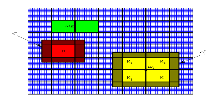
Figure 1: Illustration of fine grid, coarse grid, coarse neighborhood and oversampled domain.

1.3 The basic concepts of Generalized Multiscale Finite Element Method

General idea of GMsFEM. In this paper, we will develop novel solution strategies centered around adaptive multiscale model reduction. The GMsFEM was first presented in [32] and later investigated in several other papers (e.g., [43, 44, 33, 35, 8, 25, 26, 23, 24]). The GMsFEM is motivated by our earlier works on designing multiscale coarse spaces for domain decomposition preconditioners [42, 31, 34], the studies in MsFEM, and the concepts of global model reduction methods (e.g., [49, 5] and references therein), which employ global snapshots and Proper Orthogonal Decomposition (POD). The proposed approach is a generalization of the MsFEM and defines appropriate local snapshots and local spectral decompositions. The need for such systematic methods will be discussed in the examples of various applications. Our proposed approaches add local degrees of freedom as needed and provide numerical macroscopic equations for problems without scale separation and high contrast. Because of the proposed multiscale model reduction’s local nature of, one can adaptively add the degrees of freedom based on error estimators and rigorously estimate the errors. To our best knowledge, this is one of the first local systematic multiscale model reduction frameworks that can be easily adopted for different applications.

Multiscale basis functions and snapshot spaces. The main idea of our multiscale approach is to systematically select important degrees of freedom for the solution in each coarse block (see Figure 1 for coarse and fine grid illustration). More precisely, for each coarse block $\omega_{i}$ (or $K$), we identify local multiscale basis functions $\phi_{j}^{\omega_{i}}$ ($j=1,...,N_{\omega_{i}}$) and seek the solution in the span of these basis functions. For problems with scale separation, one needs a limited number of degrees of freedom. However, as the heterogeneities get more complicated, one needs a systematic approach to find the additional degrees of freedom. In each coarse grid, we first build the snapshot space, $V_{\text{snap}}^{\omega_{i}}=\text{span}\{\psi_{j}^{\omega_{i}}$}. The choice of the snapshot space depends on the global discretization and the particular application. The appropriate snapshot space (1) yields faster convergence, (2) imposes problem relevant restrictions on the coarse spaces (e.g., divergence free solutions) and (3) reduces the computational cost of building the offline spaces. Each snapshot can be constructed, for example, using random boundary conditions or source terms [9].

Reducing the degrees of freedom. Once we construct the snapshot space $V_{\text{snap}}^{\omega_{i}}$, we identify the offline space, which is a principal component subspace of the snapshot space and derived based on analysis. To obtain the offline space, we perform a dimension reduction of the snapshot space. This reduction identifies dominant modes, which we use to construct a multiscale space. If the snapshot space and the local spectral problems are appropriately chosen, we obtain reduced dimensional spaces corresponding to numerical homogenization in the case of scale separation. When there is no scale separation, we have a constructive method to add the necessary extra degrees of freedom that capture the relevant interactions between scales.

Adaptivity and nonlinearities. The algorithmic framework proposed above is general and can be used for different multiscale, high contrast, and perforated problems [22, 26, 43, 8]. The multiscale basis functions are constructed locally and using an adaptive criteria. Thus, in different regions, we expect a different number of basis functions depending on the local features of the problem, such as heterogeneities and high contrast. For example, in the regions with scale separation, we expect only a limited number of degrees of freedom. The adaptivity will be achieved using error indicators. In nonlinear problems, one performs local nonlinear interpolation to approximate the Jacobian or other nonlinear terms. The above multiscale procedure can be complemented with online basis functions which helps to converge to the fine-scale solution by constructing multiscale basis functions in the simulations [23, 24] (also, see Figure 2 for the ingredients of proposed multiscale method).

Limitations. Though the proposed approaches can be used in many applications, it is limited to problems where the solution space locally has a low dimensional structure. If the latter is not the case, our approaches will use many degrees of freedom and the computational gain may not be significant in those regions. Many multiscale application problems we have encountered can benefit from local adaptive multiscale model reduction.

1.3.1 Methodological ingredients of GMsFEM

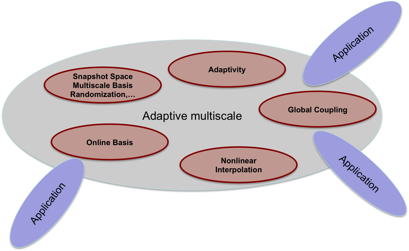
Figure 2: Multiscale model reduction. Ingredients and Applications.

Our computational framework will rely on several important ingredients (see Figure 2) that are general for various discretizations (such as mixed methods, discontinuous Galerkin, and etc,) and applications. These ingredients include (1) a procedure for identifying local snapshot spaces and multiscale basis, (2) developing global coupling mechanisms for multiscale basis functions, (3) adaptivity strategies, (4) local nonlinear interpolation tools, and (5) online basis functions. These ingredients are building blocks that are needed for constructing an accurate and robust multiscale model reduction. We will motivate the use of multiscale model reduction by showing how it can take us beyond conventional macroscopic modeling and discuss some relevant ingredients.

The proposed framework provides a promising tool and capability for solving a large class of multiscale problems without scale separation and high contrast. This framework is tested and applied in various applications where we have followed the general framework to construct local multiscale spaces. We identify main ingredients of the framework, which can be further investigated for speed-up and accuracy.

1.4 Applications and organization of the paper

We apply the proposed adaptive multiscale framework to several challenging and distinct applications where one deals with a rich hierarchy of scales. These include (1) flows in heterogeneous porous media (2) diffusion in fractured media (3) multiscale processes in perforated regions (4) wave propagation in heterogeneous media (5) nonlinear diffusion equations in heterogeneous media. We will discuss some of the applications here.

In Section 2, we describe numerical homogenization and its limitations. In Section 3, we discuss Multiscale Finite Element Method. In Section 4, we describe the GMsFEM and its basic principles. In Section 5, adaptive strategies for the GMsFEM are described. Section 6 is devoted to the construction of the online basis functions. We describe the selected global couplings in Section 7. The GMsFEM using sparsity in the snapshot space is discussed in Section 8. We discuss the GMsFEM for space-time heterogeneous problems in Section 9. In Section 10, we discuss the GMsFEM for problems in perforated domains. We present some selected applications in Section 11. In Section 12, we discuss some remaining aspects of the GMsFEM, such as applications to nonlinear problems and its use in global model reduction techniques.

2 A brief introduction to numerical homogenization

2.1 Numerical homogenization

The main idea of numerical homogenization is to identify the homogenized coefficients in each coarse-grid block. The basic underlying principle is to compute these upscaled quantities such that they preserve some averages for a given set of local boundary conditions. We discuss it on an example.

We consider a simple example

$$\frac{\partial}{\partial x_{i}}\left(\kappa_{ij}(x)\frac{\partial}{\partial x_{j}}u\right)=f,$$ (2)

where $\kappa_{ij}(x)$ is a heterogeneous field. The objective is to define an upscaled (or homogenized) conductivity for each coarse block without directly using the periodicity. Following the homogenization technique, the local problems are solved in each coarse block

$$\frac{\partial}{\partial x_{i}}\left(\kappa_{ij}(x)\frac{\partial}{\partial x_{j}}\mathcal{N}_{l}\right)=0\ \text{in}\ K,$$ (3)

where $K$ is a coarse block. The boundary condition needs to be chosen such that it represents the local heterogeneities. We limit ourselves to Dirichlet boundary conditions ${\mathcal{N}}_{l}=x_{l}$ on $\partial K$. One can use other boundary conditions [68].

We note that if the local problem is homogenized and the homogenized coefficients are constant, then the solution of the homogenized equation is $\mathcal{N}_{l}^{*}=x_{l}$ in $K$. The upscaled coefficients $\kappa^{*,nh}_{ij}$ can be defined by averaging the fluxes:

$$\int_{K}\kappa_{ij}^{*,nh}\frac{\partial}{\partial x_{j}}\mathcal{N}_{l}^{*}=\int_{K}\kappa_{ij}(x)\frac{\partial}{\partial x_{j}}\mathcal{N}_{l}.$$ (4)

The motivation behind this upscaling is to state that the average flux response for the fine-scale local problem with prescribed boundary conditions is the same as that for the upscaled solution. If we take $\mathcal{N}_{l}^{*}=x_{l}\ \text{in}\ \ K$, we have

$$\kappa_{il}^{*,nh}={1\over|K|}\int_{K}\kappa_{ij}(x)\frac{\partial}{\partial x_{j}}\mathcal{N}_{l}.$$ (5)

Remark 1 (Convergence).

Assuming that $\kappa_{ij}(x)=\kappa_{ij}(x/\epsilon)$, one can study the convergence of the numerical homogenization technique and show ([68]) that

$$|\kappa_{il}^{*,nh}-\kappa_{il}^{*}|\leq C\sqrt{\epsilon\over H},$$

where $\kappa_{il}^{*,nh}$ is the numerical homogenization and $\kappa_{il}^{*}$ is the “correct” homogenized coefficients.

Remark 2 (Oversampling).

The convergence analysis suggests that the boundary layers due to artificial linear boundary conditions, $\mathcal{N}_{l}=x_{l}$, cause the resonance errors. To reduce these resonance errors, oversampling technique has been proposed. The main idea of this method is to solve local problems in a larger domain. In oversampling method [50], the local problem that is analogous to (3) is solved in a larger domain (see Figure 1). In particular, if we denote the large domain by $K^{+}$ while the target coarse block by $K$ (see Figure 1), then

$$\frac{\partial}{\partial x_{i}}\left(\kappa_{ij}(x)\frac{\partial}{\partial x_{j}}\mathcal{N}_{l}^{ovs}\right)=0\ \text{in}\ K^{+}.$$ (6)

For simplicity, we can use $\mathcal{N}_{l}^{ovs}=x_{l}\ \text{on}\ \partial K^{+}$. The upscaled conductivity $\kappa^{*,ovs}_{ij}$ is computed by equating the fluxes on the target coarse block:

$$\int_{K}\kappa_{ij}^{*,ovs}\frac{\partial}{\partial x_{j}}\mathcal{N}_{l}^{*,ovs}=\int_{K}\kappa_{ij}(x)\frac{\partial}{\partial x_{j}}\mathcal{N}_{l}^{ovs}.$$ (7)

Noting that the domain $K^{+}$ is only slightly larger, we can still claim that $\mathcal{N}_{l}^{*,ovs}=x_{l}$, and thus,

$$\kappa_{il}^{*,ovs}={1\over|K|}\int_{K}\kappa_{ij}(x)\frac{\partial}{\partial x_{j}}\mathcal{N}_{l}^{ovs}.$$ (8)

The advantage of this approach is that one reduces the effects of the oscillatory boundary conditions. One can show ([68]) that the error for the residual is small and scales as $\epsilon/H$ instead of $\sqrt{\epsilon/H}$.

2.2 Limitations

The above numerical homogenization concepts (for linear and nonlinear problems) are often used to derive macroscopic equations. These techniques assume that the solution space has a reduced dimensional structure. For example, as we can observe from the above example and derivations, the solution in each coarse block is approximated by three local fields (in 3D). In fact, this “effective” dimension is related to the number of elements (constants) in the effective properties. In general, for many macroscopic equations, one implicitly assumes the local effective dimension for the solution space related to the number of macroscopic parameters. In many cases, the assumptions on the limited effective dimension of microscale problem break down and the local solution space may need more degrees of freedom. This requires general approaches, where we do not rely on macroscale equations, and approximate the solution space via multiscale basis functions. Next, we give a brief overview of these concepts.

3 Multiscale Finite Element Method

In this section, we will give a brief overview of MsFEM as a method for solving a problem on a coarse grid. MsFEMs consist of two major ingredients: (1) multiscale basis functions and (2) a global numerical formulation which couples these multiscale basis functions. Multiscale basis functions are designed to capture the fine-scale features of the solution. Important multiscale features of the solution need to be incorporated into these localized basis functions which contain information about the scales which are smaller (as well as larger) than the local numerical scale defined by the basis functions. In particular, we need to incorporate the features of the solution that can be localized and use additional basis functions to capture the information about the features that need to be separately included in the coarse space. A global formulation couples these basis functions to provide an accurate approximation of the solution.

As before, we consider the second order elliptic equations with heterogeneous coefficients

$$\mathcal{L}(u)=f,$$ (9)

where $\mathcal{L}(u)=-\frac{\partial}{\partial x_{i}}\left(\kappa_{ij}(x)\frac{\partial}{\partial x_{j}}u\right)$ with appropriate boundary conditions. We seek multiscale basis functions supported in each domain $\omega_{j}$, denoted by $\phi^{\omega_{j}}$. Then, the coarse-grid solution is represented by

$$u_{H}=\sum_{i}c_{i}\phi^{\omega_{i}},$$

where $c_{i}$ are determined from

$$a(u_{H},v_{H})=(f,v_{H}),\quad\text{for all}\ v_{H}\in V_{0}.$$ (10)

In the above formulation, we define $V_{0}=\text{span}\{\phi^{\omega_{i}}\}$,

$$a(u,v)=\int_{\Omega}\kappa(x)\nabla u(x)\nabla v(x)\quad\text{and}\quad(f,v)=\int_{\Omega}f(x)v(x).$$ (11)

One can also view MsFEM in the discrete setting. Assume that the basis functions are defined on a fine grid as $\Phi^{\omega_{i}}$ with $i$ varying from $1$ to $N_{c}$, where $N_{c}$ is the number of multiscale basis functions. Given coarse-scale basis functions, the coarse space is given by

$$V_{0}=\mbox{span}\{\Phi^{\omega_{i}}\}_{i=1}^{N_{c}},$$ (12)

and the coarse matrix is given by $A_{H}=R_{0}^{T}AR_{0}$ where $A$ is the fine-scale stiffness matrix and

$$R_{0}=[\Phi^{\omega_{1}},\dots,\Phi^{\omega_{N_{c}}}].$$

Here $\Phi^{\omega_{i}}$’s are discrete coarse-scale basis functions defined on a fine grid (i.e., column vectors). Multiscale finite element solution is the finite element projection of the fine-scale solution into the space $V_{0}$. More precisely, multiscale solution $U_{H}$ is given by

$$A_{H}u_{H}=f_{H},$$

where $f_{H}=R_{0}^{T}b$. Next, we discuss some coarse spaces.

Linear boundary conditions. Let $\chi_{i}^{0}$ be the standard piecewise linear or piecewise polynomial basis function supported in $\omega_{i}$. We define multiscale finite element basis functions that coincide with $\chi_{i}^{0}$ on the boundaries of the coarse partition. In particular,

$$\mbox{div}(\kappa\nabla\chi_{i}^{ms})=0\ \ \mbox{in }K\in\omega_{i},\quad\chi_{i}^{ms}=\chi_{i}^{0}\ \ \mbox{in }\partial K,\ \ \forall\ K\subset\omega_{i},$$ (13)

where $K$ is a coarse grid block within $\omega_{i}$. Note that multiscale basis functions coincide with standard finite element basis functions on the boundaries of coarse grid blocks, while are oscillatory in the interior of each coarse grid block.

Remark 3.

We would like to remark that the MsFEM formulation allows one to take advantage of scale separation. In particular, $K$ can be chosen to be a volume smaller than the coarse grid and the integrals in the stiffness matrix computations need to be re-scaled (see [37] for discussions).

Remark 4 (The relation between MsFEM and numerical homogenization).

It can be shown ([37]) that the MsFEM with one basis function on triangular elements yields the same coarse-grid stiffness matrix as the numerical homogenization.This is due to the fact that the numerical homogenization uses the local solutions of PDEs as in the MsFEM. However, the MsFEM has several advantages, which include fine-scale information recovery, adaptivity based on the residual, the use of global information and so on ([37]).

Remark 5 (The relation between MsFEM and some other multiscale techniques).

The relation between the MsFEM and other multiscale methods is discussed in [37]. It can be shown that the MsFEM can use an approximation of multiscale basis functions if there is a periodicity. As a result, the MsFEM can recover a similar approximation and the computational cost as Heterogeneous Multiscale Method ([29]) for elliptic equations in the presence of scale separation. The relation of the MsFEM and variational multiscale method ([53]) is also discussed in [37]. The variational multiscale method (VMM) recovers the fine-scale information via the equation for the residual. The localization of this equation and the choice of the initial multiscale spaces are important for the VMM. It can be shown that with a simple choice, one can recover the MsFEM. On the other hand, one can use more sophisticated coarse spaces and the residual recovery, to improve the accuracy of the VMM [10].

Oversampling technique. Because of linear boundary conditions, the basis functions do not capture the fine-scale features of the solution along the boundaries. This can lead to large errors. When coefficients have a single physical scale $\epsilon$, it has been shown that the error (see [52]) is proportional to $\epsilon/H$, and thus can be large when $H$ is close to $\epsilon$. Motivated by such examples, Hou and Wu in [50] proposed an oversampling technique for multiscale finite element method. Specifically, let $\psi^{+,\omega_{i}}$ be the basis functions satisfying the homogeneous elliptic equation in the larger domain $K^{+}\supset K$ (see Figure 1). We then form the actual basis $\phi^{+,\omega_{i}}$ by linear combination of $\psi^{+,\omega_{i}}$, $\phi^{+,\omega_{i}}=\sum_{j}\alpha_{ij}\psi^{+,\omega_{j}}$, and restricting them to $K$. The coefficients $\alpha_{ij}$ are determined by condition $\phi^{+,\omega_{i}}(x_{j})=\delta_{ij}$, where $x_{j}$ are nodal points. Other conditions can also be imposed (e.g., $\alpha_{ij}$ are determined based on homogenized parts of $\psi^{+,\omega_{i}}$). Note that this method is non-conforming. One can also multiply the oversampling functions by linear basis functions to restrict them onto $\omega_{i}$ and have a conforming method. Numerical results and more discussions on oversampling methods can be found in [37]. Many other boundary conditions are introduced and analyzed in the literature. For example, reduced boundary conditions are found to be efficient in many porous media applications ([54]).

The use of limited global information. Previously, we discussed multiscale methods which employ local information in computing basis functions with the exception of energy minimizing basis functions. The accuracy of these approaches depends on local boundary conditions. Though effective in many cases, multiscale methods that only use local information may not accurately capture the local features of the solution. In a number of previous papers, multiscale methods that employ limited global information is introduced. The main idea of these multiscale methods is to incorporate some fine-scale information about the solution that can not be computed locally and that is given globally. More precisely, in these approaches, we assume that the solution can be represented by a number of fields $p_{1}$,…, $p_{N}$, such that

$$u\approx G(p_{1},...,p_{N}),$$ (14)

where $G$ is sufficiently smooth function, and $p_{1}$,.., $p_{N}$ are global fields. These fields typically contain the essential information about the heterogeneities at different scales and can also be local fields defined in larger domains. In the above assumption (14), $p_{i}$ are solutions of elliptic equations. These global fields are used to construct multiscale basis functions (often multiple basis functions per a coarse node). Finding $p_{1}$, …, $p_{N}$, in general, can be a difficult task and we refer to Owhadi and Zhang [62] as well as to [36] where various choices of global information are proposed.

4 Generalized Multiscale Finite Element Method. Basic Concepts

4.1 Overview

Previous multiscale finite element concepts focus on constructing one basis function per node. As we discussed earlier these approaches are similar to numerical homogenization (upscaling), i.e., one can use one basis function to localize the effects of local heterogeneities. However, for many complex heterogeneities, multiple basis functions are needed to represent the local solution space. For example, if the coarse region contains several high-conductivity regions, one needs multiple multiscale basis functions to represent the local solution space. In this section, we discuss how to systematically construct multiscale basis functions in a general framework Generalized Multiscale Finite Element Methods.

Generalized Multiscale Finite Element Method (GMsFEM) incorporates complex input space information and the input-output relation. It systematically enriches the coarse space through our local construction. Our approach, as in many multiscale and model reduction techniques, divides the computation into two stages (see Figure 3): offline and online. In the offline stage, we construct a small dimensional space that can be efficiently used in the online stage to construct multiscale basis functions. These multiscale basis functions can be re-used for any input parameter to solve the problem on a coarse-grid. Thus, this provides a substantial computational saving in the online stage. Below, we present an outline of the algorithm and will discuss its main ideas on the example of (9).

Offline computations: (1) Coarse grid generation; (2) Construction of snapshot space that will be used to compute an offline space. (3) Construction of a small dimensional offline space by performing dimension reduction in the space of snapshots.

Online computations: (1) For each input parameter, compute multiscale basis functions (for parameter dependent problems); (2) Solution of a coarse-grid problem for any force term and boundary condition; (3) Iterative solvers, if needed.

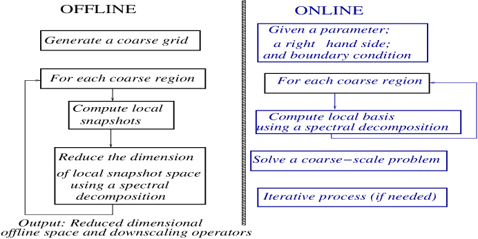
Figure 3: Flow chart

4.2 Examples of snapshot spaces. Oversampling and non-oversampling

The snapshot space, denoted by $V_{H,\text{snap}}^{\omega_{i}}$ for a generic domain $\omega_{i}$, is defined for each coarse region $\omega_{i}$ (with elements of the space denoted $\psi_{l}^{\omega_{i}}$) and can approximate the solution space with a prescribed accuracy. The appropriate snapshot space (1) yields faster convergence, (2) imposes problem relevant restrictions on the coarse spaces (e.g., divergence free solutions) and (3) reduces the computational cost of building the offline spaces. In particular, we emphasize that the use of oversampling in the snapshot spaces can improve the convergence.

4.2.1 All fine-grid functions

We can use local fine-scale spaces consisting of fine-grid basis functions within a coarse region. More precisely, the snapshot vectors consists of unit vectors defined on a fine grid within a coarse region. In this case, the offline spaces will be computed on a fine grid directly ([31]).

4.2.2 Harmonic extensions

This choice of snapshot space consists of harmonic extension of fine-grid functions defined on the boundary of $\omega_{i}$. More precisely, for each fine-grid function, $\delta_{l}^{h}(x)$, which is defined by $\delta_{l}^{h}(x_{k})=\delta_{l,k},\,\forall x_{k}\in\textsl{J}_{h}(\omega_{i})$, where $\textsl{J}_{h}(\omega_{i})$ denotes the set of fine-grid boundary nodes on $\partial\omega_{i}$, we obtain a snapshot function $\psi_{l}^{\omega_{i}}$ by

$$\mathcal{L}(\psi_{l}^{\omega_{i}})=0\ \ \text{in}\ \omega_{i}$$

subject to the boundary condition, $\psi_{l}^{\omega_{i}}=\delta_{l}^{h}(x)$ on $\partial\omega_{i}$. Here $\delta_{l,k}=1$ if $l=k$ and $\delta_{l,k}=0$ if $l\neq k$.

4.2.3 Oversampling approaches

To describe the oversampling approach, we consider the harmonic extension as described above in the oversampled region (see, e.g., Figure 1). This choice of snapshot space consists of harmonic extension of fine-grid functions defined on the boundary of $\omega_{i}^{+}$. More precisely, for each fine-grid function, $\delta_{l}^{h}(x)$, which is defined by $\delta_{l}^{h}(x_{k})=\delta_{l,k},\,\forall x_{k}\in\textsl{J}_{h}(\omega_{i}^{+})$, where $\textsl{J}_{h}(\omega_{i}^{+})$ denotes the set of fine-grid boundary nodes on $\partial\omega_{i}^{+}$, we obtain a snapshot function $\psi_{l}^{+,\omega_{i}}$ by

$$\mathcal{L}(\psi_{l}^{+,\omega_{i}})=0\ \ \text{in}\ \omega_{i}^{+}$$

subject to the boundary condition, $\psi_{l}^{+,\omega_{i}}=\delta_{l}^{h}(x)$ on $\partial\omega_{i}^{+}$.

4.2.4 Randomized boundary conditions

In the above construction of snapshot vectors, many local problems are solved. This is not necessary and one can only solve a relatively small number of snapshot vectors. The number of snapshot vectors is defined by the number of offline multiscale basis functions. In this case, we will use random boundary conditions.

More precisely, for each fine-grid function, $r_{l}^{h}(x)$, which is defined by $r_{l}^{h}(x_{k})=r_{l,k},\,\forall x_{k}\in\textsl{J}_{h}(\omega_{i}^{+})$, where $r_{l,k}$ are random numbers, we obtain a snapshot function $\psi_{l}^{+,\omega_{i}}$ by

$$\mathcal{L}(\psi_{l}^{+,\omega_{i}})=0\ \ \text{in}\ \omega_{i}^{+}$$

subject to the boundary condition, $\psi_{l}^{+,\text{snap}}=r_{l}^{h}(x)$ on $\partial\omega_{i}^{+}$.

4.3 Offline spaces

The offline space, denoted by $V_{H,\text{off}}^{\omega_{i}}$ for a generic domain $\omega_{i}$, is defined for each coarse region $\omega_{i}$ (with elements of the space denoted $\phi_{l}^{\omega_{i}}$) and used to approximate the solution. The offline space is constructed by performing a spectral decomposition in the snapshot space and selecting the dominant eigenvectors (corresponding to the smallest eigenvalues). The choice of the spectral problem is important for the convergence and is derived from the analysis as it is described below. The convergence rate of the method is proportional to $1/\Lambda_{*}$, where $\Lambda_{*}$ is the smallest eigenvalue among all coarse blocks whose corresponding eigenvector is not included in the offline space. Our goal is to select the local spectral problem to remove as many small eigenvalues as possible so that we can obtain smaller dimensional coarse spaces to achieve a higher accuracy.

4.3.1 General concept and example

The construction of the offline space requires solving an appropriate local spectral eigenvalue problem. The local spectral problem is derived from the analysis. A first step in the analysis is to decompose the energy functional corresponding to the error into coarse subdomains. For simplicity, we denote the energy functional corresponding to the domain $\Omega$ by $a_{\Omega}(u,u)$, e.g., $a_{\Omega}(u,u)=\int_{\Omega}\kappa\nabla u\cdot\nabla u$. Then,

$$\begin{split}a_{\Omega}(u-u_{H},u-u_{H})\preceq\sum_{\omega}a_{\omega}(u^{\omega}-u_{H}^{\omega},u^{\omega}-u_{H}^{\omega}),\end{split}$$ (15)

where $\omega$ are coarse regions ($\omega_{i}$), $u^{\omega}$ is the localization of the solution using the snapshot vectors defined for $\omega$ and $u_{H}^{\omega}$ is the component of the solution $u_{H}$ spanned by the basis in $\omega$.

The local spectral decomposition is chosen to bound $a_{\omega}(u^{\omega}-u_{H}^{\omega},u^{\omega}-u_{H}^{\omega})$. We seek the subspace $V_{H,\text{off}}^{\omega}$ (since $u^{\omega}\in V_{H,\text{snap}}^{\omega}$) such that for any $\psi\in V_{H,\text{snap}}^{\omega}$, there exists $\psi_{0}\in V_{H,\text{off}}^{\omega}$ with,

$$a_{\omega}(\psi-\psi_{0},\psi-\psi_{0})\preceq{\delta}s_{\omega}(\psi-\psi_{0},\psi-\psi_{0}),$$ (16)

where $s_{\omega}(\cdot,\cdot)$ is an auxiliary bilinear form, which needs to be chosen and $\delta$ is a threshold related to eigenvalues. First, we would like the fine-scale solution to be bounded in $s_{\omega}(\cdot,\cdot)$. We note that, in computations, (16) involves solving a generalized eigenvalue problem with a mass matrix defined using $s_{\omega}(\cdot,\cdot)$ and the basis functions are selected based on dominant eigenvalues as described above. The threshold value $\delta$ is chosen based on the eigenvalue distribution. Secondly, we would like the eigenvalue problem to have a fast decay in the spectrum (this typically requires using oversampling techniques). Thirdly, we would like to bound

$$\sum_{\omega}s_{\omega}(u^{\omega}-u_{H}^{\omega},u^{\omega}-u_{H}^{\omega})\preceq\widetilde{a}_{\Omega}(u,u),$$

where $\widetilde{a}_{\Omega}(u,u)$ can be bounded independent of physical parameters and the mesh sizes. In this step, one can need energy minimizing snapshots (See Remark 8 and [18]).

Next, we discuss a choice for $a_{\omega}(\cdot,\cdot)$ and $s_{\omega}(\cdot,\cdot)$. Recall that for (16), we need a a local spectral problem, which is to find a real number $\lambda$ and $v\in V_{H,\text{snap}}^{\omega_{i}}$ such that

$$a_{\omega_{i}}(v,w)=\lambda s_{\omega_{i}}(v,w),\qquad\forall w\in V_{H,\text{snap}}^{\omega_{i}},$$ (17)

where $a_{\omega_{i}}$ is a symmetric non-negative definite bilinear operator and $s_{\omega_{i}}$ is a symmetric positive definite bilinear operators defined on $V_{H,\text{snap}}^{\omega_{i}}\times V_{H,\text{snap}}^{\omega_{i}}$. Based on our analysis, we can choose

$$a_{\omega_{i}}(v,w)=\int_{\omega_{i}}\kappa\nabla v\cdot\nabla w,\ s_{\omega_{i}}(v,w)=\int_{\omega_{i}}\widetilde{\kappa}vw,$$

where $\widetilde{\kappa}=\sum_{i=1}^{N_{c}}\kappa\nabla\chi_{i}^{ms}\cdot\nabla\chi_{i}^{ms}$ and $\chi_{i}^{ms}$ are multiscale basis functions (see (13)). We let $\lambda_{j}^{\omega_{i}}$ be the eigenvalues of (17) arranged in ascending order. We will use the first $l_{i}$ eigenfunctions to construct our offline space $V_{H,\text{off}}^{\omega_{i}}$. The choice of the eigenvalue problem is motivated by the convergence analysis. The convergence rate is proportional to $1/\Lambda_{*}$ (with the proportionality constant depending on $H$), where $\Lambda_{*}$ is the smallest eigenvalue that the corresponding eigenvector is not included in the offline space. We would like to remove as many small eigenvalues as possible. The eigenvectors of the corresponding small eigenvalues represent important features of the solution space. By choosing the multiscale basis functions, $\chi_{i}^{ms}$, in the construction of local spectral problem, some localizable important features are taken into consideration through $\chi_{i}^{ms}$ and, as a result, we have fewer small eigenvalues (see [31] for more discussions).

For constructing conforming multiscale basis functions, the selected eigenfunctions are multiplied by the partition of unity functions, such as $\chi_{i}^{ms}$ or $\chi_{i}^{0}$ (cf., [60]). The multiplication by the partition of unity functions modifies the multiscale nature of the selected multiscale eigenfunctions. We will discuss some other important discretizations such as mixed, discontinuous Galerkin discretizations, which can be more suitable for the coupling of the multiscale eigenfunctions and which avoid the multiplication by the partition of unity functions. The global offline space $V_{H,\text{off}}$ is formed as the union of all $V_{H,\text{off}}^{\omega_{i}}$. Once the offline space is constructed, we solve (10) and find $u_{H}=\sum c_{i,j}\phi_{j}^{\omega_{i}}\in V_{H,\text{off}}$ such that

$$a(u_{H},v_{H})=(f,v_{H}),\ \forall v_{H}\in V_{H,\text{off}}.$$ (18)

4.3.2 An implementation view

Next, we present an implementation view of the local spectral decomposition. The space formed by the snapshot vectors is

$$V_{H,\text{snap}}^{\omega_{i}}=\text{span}\{\Psi_{l}^{\omega_{i}}:\leavevmode\nobreak\ \leavevmode\nobreak\ \leavevmode\nobreak\ 1\leq l\leq L_{i}\},\ \ V_{H,\text{snap}}^{+,\omega_{i}}=\text{span}\{\Psi_{l}^{+,\omega_{i}}:\leavevmode\nobreak\ \leavevmode\nobreak\ \leavevmode\nobreak\ 1\leq l\leq L_{i}^{+}\}$$

for each coarse neighborhood $\omega_{i}$ and for each oversampled coarse neighborhood $\omega_{i}^{+}$, respectively, where $L_{i}$ and $L_{i}^{+}$ are the dimensions of the snapshot spaces $V_{H,\text{snap}}^{\omega_{i}}$ and $V_{H,\text{snap}}^{+,\omega_{i}}$. We note that in the case when $\omega_{i}$ is adjacent to the global boundary, no oversampled domain is used. We can put all snapshot functions using a matrix representation

$$R_{\text{snap}}^{\omega_{i}}=\left[\Psi_{1}^{\omega_{i}},\ldots,\Psi_{L_{i}}^{\omega_{i}}\right],\quad R_{\text{snap}}^{+,\omega_{i}}=\left[\Psi_{1}^{+,\omega_{i}},\ldots,\Psi_{L_{i}^{+}}^{+,\omega_{i}}\right],$$

The local spectral problems (17) can be written in a matrix form as

$$A^{\omega_{i}}\Psi_{k}^{\omega_{i}}=\lambda_{k}^{\omega_{i}}S^{\omega_{i}}\Psi_{k}^{\omega_{i}},\quad A^{+,\omega_{i}}\Psi_{k}^{\omega_{i}}=\lambda_{k}^{\omega_{i}}S^{+,\omega_{i}}\Psi_{k}^{\omega_{i}}$$ (19)

for the $k$-th eigenpair. We present two choices: one with no oversampling and one with oversampling, though one can consider various options [35]. In (19), with no oversampling, we can choose $A^{\omega_{i}}=[a^{\omega_{i}}_{mn}]$ and $S^{\omega_{i}}=[s^{\omega_{i}}_{mn}]$, where $a^{\omega_{i}}_{mn}=\int_{\omega_{i}}{\kappa}\nabla\psi_{m}^{\omega_{i}}\cdot\nabla\psi_{n}^{\omega_{i}}=(R^{\omega_{i}}_{\text{snap}})^{T}{A}R^{\omega_{i}}_{\text{snap}}$ and  and $s^{\omega_{i}}_{mn}=\int_{\omega_{i}}\widetilde{{\kappa}}\,\psi_{m}^{\omega_{i}}\,\psi_{n}^{\omega_{i}}=(R^{\omega_{i}}_{\text{snap}})^{T}{S}R_{\text{snap}}^{\omega_{i}}$. With oversampling, we can choose $A^{+,\omega_{i}}=[a^{+,\omega_{i}}_{mn}]$ and $S^{+,\omega_{i}}=[s^{+,\omega_{i}}_{mn}]$, where $a^{+,\omega_{i}}_{mn}=\int_{\omega_{i}^{+}}{\kappa}\nabla\psi_{m}^{+,\omega_{i}}\cdot\nabla\psi_{n}^{+,\omega_{i}}=(R^{+,\omega_{i}}_{\text{snap}})^{T}{A}R^{+,\omega_{i}}_{\text{snap}}$ and $s^{+,\omega_{i}}_{mn}=\int_{\omega_{i}^{+}}\widetilde{{\kappa}}\,\psi_{m}^{+,\omega_{i}}\,\psi_{n}^{+,\omega_{i}}=(R^{+,\omega_{i}}_{\text{snap}})^{T}{S}R_{\text{snap}}^{+,\omega_{i}}$. To generate the offline space we then choose the smallest $l_{i}$ eigenvalues and form the corresponding eigenvectors in the respective space of snapshots by setting $\phi_{k}^{\omega_{i}}=\sum_{j=1}^{L_{i}}\Psi_{kj}^{\omega_{i}}\psi_{j}^{\omega_{i}}$ or $\phi_{k}^{+,\omega_{i}}=\sum_{j=1}^{L_{i}^{+}}\Psi_{kj}^{+,\omega_{i}}\psi_{j}^{+,\omega_{i}}$ (for $k=1,\ldots,L_{i}$ or $k=1,\cdots,L_{i}^{+}$), where $\Psi_{kj}^{\omega_{i}}$ and $\Psi_{kj}^{+,\omega_{i}}$ are the coordinates of the vector $\Psi_{k}^{\omega_{i}}$ and $\Psi_{k}^{+,\omega_{i}}$ respectively. Collecting all offline basis functions and using a single index notation, we then create the offline matrices $R_{\text{off}}^{+}=\left[\psi_{1}^{+,\text{off}},\ldots,\psi_{M_{\text{off}}}^{+,\text{off}}\right]$ and $R_{\text{off}}=\left[\psi_{1}^{\text{off}},\ldots,\psi_{M_{\text{off}}}^{\text{off}}\right]$ to be used in the online space construction, where $M_{\text{off}}$ is the total number of offline basis functions. The discrete system corresponding to (18) is

$$R_{\text{off}}^{T}AR_{\text{off}}u_{H}^{\text{discrete}}=R_{\text{off}}^{T}f$$

where $u_{H}^{\text{discrete}}$ is the discrete version of $u_{H}$.

4.4 A numerical example

We present a numerical result that demonstrate the convergence of the GMsFEM. More detailed numerical studies can be found in the literature. We consider the permeability field, $\kappa(x)$ (see (9)) that is shown in Figure 4, the source term $f=0$, and the boundary condition to be $x_{1}$. The fine grid is $100\times 100$, coarse grid is $10\times 10$. We consider the snapshot space spanned by harmonic functions in the oversampled domain (with randomized boundary conditions) and vary the number of basis functions per node. The numerical results are shown in Table 1 in which $e_{a}$ and $e_{2}$ denote errors in energy and $L^{2}$ norms repsectively. As we observe from these numerical results the GMsFEM converges as we increase the number of basis functions. We also show the convergence when using polynomial basis functions. It is clear that the FEM method with polynomial basis functions does not converge and one can only observe this convergence only after a very large number of basis functions are chosen so that we cross the fine-scale threshold. We note that the convergence with one basis function per node does not perform well for the GMsFEM because of the high contrast. The first, second, and third smallest eigenvalues, $\Lambda_{*}$, among all coarse blocks are $0.0024$, $24.0071$, $35.6941$, respectively. We emphasize that if the eigenvalue problem (and the snapshot space) is not chosen appropriately, one can get more very small eigenvalues ([31]). As we see that the first smallest eigenvalue is very small and, as a result, the error is large, when using one basis function. The eigenvalue distribution is important for online basis construction, as will be discussed later.

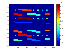
Figure 4: The permeability field $\kappa(x)$.

#basis (DOF)	$e_{a}$	$e_{2}$
1 (81)	69.05%	12.19%
2 (162)	22.55%	1.19%
3 (243)	19.86%	0.99%
4 (324)	16.31%	0.70%
5 (405)	14.20%	0.65%

DOF	$e_{a}$	$e_{2}$
81	103.2%	23%
361	100%	23%
841	80.33%	15%

Table 1: Left table: The convergence for the GMsFEM using multiscale basis functions. Right table: The convergence for FEM using polynomials basis functions.

5 Adaptivity in GMsFEM

The success of the GMsFEM depends on adaptive implementation and appropriate error indicators. In this section, we discuss an a-posteriori error indicator for the GMsFEM framework. We will demonstrate the main idea using a continuous Galerkin formulation; however, this concept can be generalized to other discretizations as we will discuss later on. This error indicator is further used to develop an adaptive enrichment algorithm for the linear elliptic equation with multiscale high-contrast coefficients. Rigorous a-posteriori error indicators are needed to perform an adaptive enrichment. We would like to point out that there are many related activities in designing a-posteriori error estimates for global reduced models. The main difference is that the error estimators presented in this section are based on a special local eigenvalue problem and use the eigenstructure of the offline space.

We can consider various kinds of error indicators that are based on the $L^{2}$-norm of the local residual and the other is based on the weighted $H^{-1}$-norm (we will also call it $H^{-1}$-norm based) of the local residual where the weight is related to the coefficient of the elliptic equation. The latter will be studied in the paper and we refer to [25] for more details.

Let $u_{H}\in V_{H,\text{off}}$ be the solution obtained in (18). Consider a given coarse neighborhood $\omega_{i}$. We define a space $V_{i}=H^{1}_{0}(\omega_{i})\cap V$ which is equipped with the norm $\|v\|_{V_{i}}^{2}=\int_{\omega_{i}}\kappa(x)|\nabla v|^{2}$. We also define the following linear functional on $V_{i}$ by

$$R_{i}(v)=\int_{\omega_{i}}fv-\int_{\omega_{i}}\kappa\nabla u_{H}\cdot\nabla v.$$ (20)

This is called the $H^{-1}$-residual on $\omega_{i}$, The functional norm of $R_{i}$, denoted by $\|R_{i}\|_{V_{i}^{*}}$, gives a measure of the size of the residual. The first important result states that these residuals give a computable indicator of the error $u-u_{H}$ in the energy norm. We have

$$\|u-u_{H}\|_{V}^{2}\leq C_{\text{err}}\sum_{i=1}^{N_{c}}\|R_{i}\|^{2}_{V_{i}^{*}}(\lambda^{\omega_{i}}_{l_{i}+1})^{-1},$$ (21)

where $C_{\text{err}}$ is a uniform constant, and $\lambda^{\omega_{i}}_{l_{i}+1}$ denotes the $({l_{i}+1})$-th eigenvalue for the problem (19) in the coarse neighborhood $\omega_{i}$, and corresponds to the first eigenvector that is not included in the construction of $V_{H,\text{off}}^{\omega_{i}}$.

The above error indicator allows one to construct an adaptive enrichment algorithm. It is an iterative process, and basis functions are added in each iteration based on the current solution. We use the index $m\geq 1$ to represent the enrichment level. At the enrichment level $m$, we use $V_{H,\text{off}}^{m}$ to denote the corresponding GMsFEM space and $u_{H}^{m}$ the corresponding solution obtained in (18) using the space $V_{H,\text{off}}^{m}$. Furthermore, we use $l_{i}^{m}$ to denote the number of basis functions used in the coarse neighborhood $\omega_{i}$. We will present the strategy for getting the space $V_{H,\text{off}}^{m+1}$ from $V_{H,\text{off}}^{m}$. Let $0<\theta<1$ be a given number independent of $m$. First of all, we compute the local residuals for every coarse neighborhood $\omega_{i}$:

$$\eta_{i}^{2}=\|R_{i}\|^{2}_{V_{i}^{*}}(\lambda^{\omega_{i}}_{l^{m}_{i}+1})^{-1},\quad\quad i=1,2,\cdots,N_{c},$$

where $R_{i}(v)$ is defined using $u_{H}^{m}$, namely,

$$R_{i}(v)=\int_{\omega_{i}}fv-\int_{\omega_{i}}\kappa\nabla u^{m}_{H}\cdot\nabla v,\quad\forall v\in V_{i}.$$

Next, we will add basis functions for the coarse neighborhoods with large residuals. To do so, we re-enumerate the coarse neighborhoods so that the above local residuals $\eta_{i}^{2}$ are arranged in decreasing order $\eta^{2}_{1}\geq\eta^{2}_{2}\geq\cdots\geq\eta^{2}_{N}$. We then select the smallest integer $k$ such that

$$\theta\sum_{i=1}^{N_{c}}\eta_{i}^{2}\leq\sum_{i=1}^{k}\eta_{i}^{2}.$$ (22)

For those coarse neighborhoods $\omega_{1},\cdots,\omega_{k}$ (in the new enumeration) chosen in the above procedure, we will add basis functions by using the next eigenfunctions $\Psi_{l_{i}+1}^{\omega_{i}},\Psi_{l_{i}+2}^{\omega_{i}},\cdots$. We remark that the number of new additional basis depends on the eigenvalue decay. The resulting space is called $V_{\text{off}}^{m+1}$. We remark that the choice of $k$ defined in (22) is called the Dorlfer’s bulk marking strategy [27].

As we mentioned the local basis functions do not contain any global information, and thus they cannot be used to efficiently capture these global behaviors. We will therefore present in the next section a fundamental ingredient of GMsFEM - the development of online basis functions that is necessary to obtain a coarse representation of the fine-scale solution and gives a rapid convergence of the corresponding adaptive enrichment algorithm.

Remark 6 (Implementation).

The algorithm above can be described as follows. We start with an initial space with a small number of basis functions for each coarse grid block. Then we solve the problem and compute the error estimator. We locate the coarse grid blocks with large errors and add more basis functions for these coarse grid blocks. This procedure is repeated until the error goes below a certain tolerance. We remark that the adaptive strategy belongs to the online process, because it is the actual simulation. On the other hand, the generation of basis functions belongs to the offline process. About stopping criteria for this algorithm, one can stop the algorithm when the total number of basis functions reach a certain level. On the other hand, one can stop the algorithm when the value of the error indicator goes below a certain tolerance.

Remark 7 (Goal Oriented Adaptivity).

For some practical problems, one is interested in approximating some function of the solution, known as the quantity of interest, rather than the solution itself. Examples include an average or weighted average of the solution over a particular subdomain, or some localized solution response. In these cases, goal-oriented adaptive methods yield a more efficient approximation than standard adaptivity, as the enrichment of degrees of freedom is focused on the local improvement of the quantity of interest rather than across the entire solution. In [30], we study goal-oriented adaptivity for multiscale methods, and in particular the design of error indicators to drive the adaptive enrichment based on the goal function. In this methodology, one seeks to determine the number of multiscale basis functions adaptively for each coarse region to efficiently reduce the error in the goal functional. Two estimators are studied. One is a residual based strategy and the other uses dual weighted residual method for multiscale problems. The method is demonstrated on high-contrast problems with heterogeneous multiscale coefficients, and is seen to outperform the standard residual based strategy with respect to efficient reduction of error in the goal function.

5.1 Numerical Results

We show numerical results for the $H^{-1}$ adaptivity. We consider the permeability field shown in Figure 4 for (9) and the forcing term shown in Figure 5. In Table 2, we present the numerical results and in Figure 5 (right plot), we compare the convergence of the adaptive GMsFEM and the GMsFEM, which uses a uniform number of basis functions. As we observe that the adaptive GMsFEM converges faster.

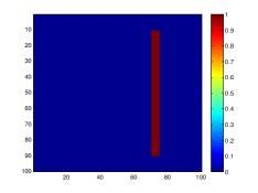
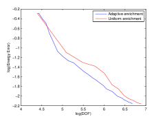
Figure 5: Left: Source function $f$. Right: The convergence of adaptive vs. uniform enrichment.

#DOF	$e_{a}$	$e_{2}$
81	75.04%	42.48%
151	30.47%	7.84%
245	22.65%	4.70%
334	18.76%	3.59%
395	16.84%	3.08%

#DOF	$e_{a}$	$e_{2}$
81	75.04%	42.48%
162	33.39%	6.74%
243	27.00%	5.52%
324	25.11%	4.72%
405	21.68%	3.50%

Table 2: Errors for the adaptive GMsFEM. Left: Adaptive enrichment. Right: Uniform enrichment.

6 Residual-based online procedure

Previously, we discussed adaptive enrichment procedures and derived an a-posteriori error indicator, which gives an estimate of the local error over coarse grid regions. We developed the error indicators based on the $L^{2}$-norm of the local residual and on the weighted $H^{-1}$-norm of the local residual, where the weight is related to the coefficient of the elliptic equation. Adaptivity is important for local multiscale methods as it identifies regions with large errors. However, after adding some initial basis functions, one needs to take into account some global information as the distant effects can be important. In this section, we discuss the development of online basis functions that substantially accelerate the convergence of GMsFEM. The online basis functions are constructed based on a residual and motivated by the analysis. We show that one needs to have a sufficient number of initial (offline) basis functions to guarantee an error decay independent of the contrast. In particular, the error decay in one adaptive iteration is proportional to $1-C\Lambda_{*}$ (see (25) for more precise estimate), where $\Lambda_{*}$ is the smallest eigenvalue among all coarse blocks that the corresponding eigenvector is not included in the offline space. Thus, it is important to include all eigenvectors corresponding to very small eigenvalues in the offline space. In general, we would like to apply one iteration of the online procedure and reach a desired error threshold. Numerical results are presented to demonstrate that one needs to have a sufficient number of initial basis functions in the offline space before constructing online multiscale basis functions.

6.1 Residual-based online adaptive GMsFEM

We use the index $m\geq 1$ to represent the enrichment level. At the enrichment level $m$, we use $V_{H,\text{off}}^{m}$ to denote the corresponding GMsFEM space and $u_{H}^{m}$ the corresponding solution. The sequence of functions $\{u_{H}^{m}\}_{m\geq 1}$ will converge to the fine-scale solution. We emphasize that the space $V_{H,\text{off}}^{m}$ can contain both offline and online basis functions. We will construct a strategy for getting the space $V_{H,\text{off}}^{m+1}$ from $V_{H,\text{off}}^{m}$. The online basis functions are computed based on some local residuals for the current multiscale solution, that is, the function $u_{H,\text{off}}^{m}$.

Suppose that we need to add a basis function $\phi^{\text{on},\omega_{i}}\in V_{i}$ on the $i$-th coarse neighbourhood $\omega_{i}$. Let $V_{H,\text{off}}^{m+1}=V_{H,\text{off}}^{m}+\text{span}\{\phi^{\text{on},\omega_{i}}\}$ be the new approximation space, and $u_{H}^{m+1}\in V_{H,\text{off}}^{m+1}$ be the corresponding GMsFEM solution. It is easy to see that $u_{H}^{m+1}$ satisfies

$$\|u-u_{H}^{m+1}\|_{V}^{2}=\inf_{v\in V_{H,\text{off}}^{m+1}}\|u-v\|_{V}^{2}.$$

Taking $v=u_{H}^{m+1}+\alpha\phi^{\text{on},\omega_{i}}$, where $\alpha$ is a scalar to be determined, we have

$$\|u-u_{H}^{m+1}\|_{V}^{2}\leq\|u-u_{H}^{m}-\alpha\phi^{\text{on},\omega_{i}}\|_{V}^{2}=\|u-u_{H}^{m}\|^{2}_{V}-2\alpha a(u-u_{H}^{m},\phi^{\text{on},\omega_{i}})+\alpha^{2}a(\phi^{\text{on},\omega_{i}},\phi^{\text{on},\omega_{i}}).$$ (23)

The last two terms in the above inequality measure the amount of reduction in error when the new basis function $\phi^{\text{on},\omega_{i}}$ is added to the space $V_{H,\text{off}}^{m}$. To determine $\phi^{\text{on},\omega_{i}}$, we first assume that the basis function $\phi^{\text{on},\omega_{i}}$ is normalized so that $a(\phi^{\text{on},\omega_{i}},\phi^{\text{on},\omega_{i}})=1$. In order to maximize the reduction in error, one can show that $\alpha=a(u-u_{H}^{m},\phi^{\text{on},\omega_{i}})$. Using this choice of $\alpha$, we have

$$\|u-u^{m+1}_{H}\|_{V}^{2}\leq\|u-u^{m}_{H}\|^{2}_{V}-|a(u-u^{m}_{H},\phi^{\text{on},\omega_{i}})|^{2}.$$

We can show that

$$a(\phi^{\text{on},\omega_{i}},v)=(f,v)-a(u^{m}_{H},v),\quad\forall v\in V_{i}$$ (24)

and $\|\phi^{\text{on},\omega_{i}}\|_{V_{i}}=\|R_{i}\|_{V_{i}^{*}}$. Hence, the new online basis function $\phi^{\text{on},\omega_{i}}\in V_{i}$ can be obtained by solving (24). In addition, the residual norm $\|R_{i}\|_{V_{i}^{*}}$ provides a measure on the amount of reduction in energy error.

In [23, 24], we have studied the convergence of the above online adaptive procedure. To simplify notations, we write $r_{i}=\|R_{i}\|_{V_{i}^{*}}$. We have shown that

$$\|u-u^{m+1}_{H}\|_{V}^{2}\leq\Big{(}1-\frac{\lambda_{n_{i}+1}^{\omega_{i}}}{C_{\text{err}}}\frac{r_{i}^{2}(\lambda_{n_{i}+1}^{\omega_{i}})^{-1}}{\sum_{j=1}^{N_{c}}r_{j}^{2}(\lambda_{n_{j}+1}^{\omega_{j}})^{-1}}\Big{)}\|u-u^{m}_{H}\|_{V}^{2},$$ (25)

where $n_{i}$ is the number of offline basis in $\omega_{i}$. The above inequality gives the convergence of the online adaptive GMsFEM with a precise convergence rate for the case when one online basis function is added per iteration. The estimate (25) shows that the eigenvectors corresponding to very small eigenvalues need to be included in the offline space in order to achieve a significant error reduction in one iteration. To enhance the convergence and efficiency of the online adaptive GMsFEM, we consider enrichment on non-overlapping coarse neighborhoods. Let $I\subset\{1,2,\cdots,N\}$ be the index set of some non-overlapping coarse neighborhoods. For each $i\in I$, we can obtain a basis function $\phi^{\text{on},\omega_{i}}\in V_{i}$ using (24). We define $V_{H,\text{off}}^{m+1}=V_{H,\text{off}}^{m}+\text{span}\{\phi^{\text{on},\omega_{i}}\,,\,i\in I\}$.

We remark that the error will decrease independent of physical parameters such as the contrast and scales if the offline space is appropriately chosen. We will demonstrate the effectiveness of this method by a numerical example. We remark that one can also derive apriori error estimate for $\|u-u^{m+1}_{H,\text{off}}\|_{V}^{2}$.

6.2 Numerical result

In Table 3, we present numerical results for online enrichment for the GMsFEM. We use the permeability field shown in Figure 4 and the forcing term shown in Figure 5 (left figure). As we observe the online enrichment does not improve the error if we have only one offline basis function. We remind that the first, second, and third smallest eigenvalues, $\Lambda_{*}$, among all coarse blocks are $0.0024$, $24.0071$, $35.6941$, respectively. Because the first eigenvalue is small, the error decrease in one online iteration is small. In particular, for each online iteration, the error decreases slightly. It is important that one adaptive online iteration can decrease the error substantially. As we increase the number of offline basis functions, the convergence is very fast and one online iteration is sufficient to reduce the error significantly. In one iteration, the error drops below $1$% for the energy error. We note that this procedure can be implemented adaptively and we add online basis functions only in some regions.

DOF\#initial basis	1	2	3		1	2	3
81	75.06%	-	-		42.49%	-	-
162	32.77%	33.50%	-		16.29%	6.76%	-
243	21.59%	1.13%	27.14%		7.33%	0.079%	5.54
324	3.46%	0.019%	1.35%		1.21%	0.0018%	0.081
405	2.45%	2.61e-04%	0.018%		0.68%	1.81e-05%	0.0011
486	1.18%	2.88e-06%	2.49e-04%		0.31%	1.74e-07%	1.60e-05%

Table 3: The errors for the GMsFEM with the online procedure (left table: $H^{1}$ errors; right table: $L^{2}$ errors).

7 Selected global discretizations and energy minimizing oversampling

In previous sections, we used continuous Galerkin coupling for multiscale basis functions. In many applications, one needs to use various discretizations. For example, for flows in porous media, mass conservation is very important and, thus, it is advantageous to use mixed methods. In seismic wave applications involving the time-explicit discretization of wave equations, one needs block-diagonal mass matrices, which can be obtained using discontinuous Galerkin approaches. In this section, we present two global couplings, mixed finite element and Interior Penalty Discontinuous Galerkin (IPDG) couplings. We refer to [39] for Hybridized Discontinuous Galerkin (HDG) coupling and to [18] for comparisons between using IPDG and HDG couplings with multiscale basis functions.

For each discretization, we define snapshot spaces and local spectral decompositions in the snapshot spaces. As we emphasized earlier the construction of the snapshot spaces and local multiscale spaces depends on the global discretization. For example, for mixed GMsFEM, the multiscale spaces are constructed for the velocity field using two neighboring coarse elements. We will present some ingredients of GMsFEM introduced earlier in the construction of multiscale basis functions, e.g., oversampling techniques and online multiscale basis functions. We also mention a new ingredient for multiscale basis construction - energy minimizing snapshots.

In a mixed formulation, the problem can be formulated as

$$\kappa^{-1}v+\nabla u=0\ \mbox{in }\Omega,\ \ \ \mbox{div}(v)=f\ \mbox{in }\Omega,$$ (26)

with Neumann boundary condition $v\cdot n=v_{\Omega}$ on $\partial\Omega$. Depending on a discretization technique, the coarse grid configuration will vary. For a mixed formulation, coarse grid blocks that share common edges (faces) will be used in constructing multiscale basis functions. In a discontinuous Galerkin formulation, the support of multiscale basis functions is limited to coarse blocks.

7.1 Discretizations

7.1.1 The mixed GMsFEM

For the mixed GMsFEM, we will construct basis functions whose supports are $\omega_{E}$, which are the two coarse elements that share a common edge (face) $E$. In particular, we let $\mathcal{E}^{H}$ be the set of all edges (faces) of the coarse grid and let $N_{e}$ be the total number of edges (faces) of the coarse grid. We define the coarse grid neighborhood $\omega_{E}$ of a face $E\in\mathcal{E}^{H}$ as

$$\omega_{E}=\bigcup\{K\in\mathcal{T}^{H}:E\in\partial K\},\quad i=1,2,\cdots,N_{e},$$

which is a union of two coarse grid blocks if $E_{i}$ is an interior edge (face) (see Figure 1). For a coarse edge $E_{i}$, we write $\omega_{E_{i}}=\omega_{i}$ to unify the notations.

Next, we define the notations for the solution spaces for the pressure $u$ and the velocity $v$. Let $Q_{H,\text{off}}$ be the space of functions which are constant on each coarse grid block. We will use this space to approximate $u$. For the multiscale approximation of the velocity $v$, we will follow the general framework of the GMsFEM and construct a multiscale space $V_{H,\text{off}}$ for the velocity. Using the pressure space $Q_{H,\text{off}}$ and the velocity space $V_{H,\text{off}}$, we solve for $u_{H}\in Q_{H,\text{off}}$ and $v_{H}\in V_{H,\text{off}}$ such that

$$\int_{\Omega}\kappa^{-1}v_{H}\cdot w-\int_{\Omega}\mbox{div}(w)u_{H}=0,\ \forall w\in\dot{V}_{H,\text{off}},\quad\int_{\Omega}\mbox{div}(v_{H})q=\int_{\Omega}fq,\ \forall q\in Q_{H,\text{off}},$$ (27)

with boundary condition $v_{H}\cdot n=v_{\Omega,H}$ on $\partial\Omega$, where $\dot{V}_{H,\text{off}}=\{v\in V_{H,\text{off}}:v\cdot n=0\mbox{ on }\partial\Omega\}$, and $v_{\Omega,H}$ is the projection of $v_{\Omega}$ in the multiscale space. We remark that we will define the snapshot and offline spaces so that the functions in $V_{H,\text{off}}$ are globally $H(\text{div})$-conforming, and as a result the normal components of the basis are continuous across coarse grid edges.

7.1.2 DG GMsFEM (GMsDGM)

For the GMsDGM, the general methodology for the construction of multiscale basis functions is similar to the above mixed GMsFEM. We will construct multiscale basis functions for the approximation of $u$ in (9). The main difference is that the functions in the snapshot space $V_{H,\text{snap}}$ and the offline space $V_{H,\text{off}}$ are supported in coarse element $K$, instead of the coarse neighborhood $\omega_{i}$. Moreover, in the oversampling approach, the oversampled regions $K^{+}$ are defined by enlarging coarse elements $K$ (see Figure 1). The construction of basis functions will be given in the next section. When the offline space $V_{H,\text{off}}$ is available, we can find the solution $u_{H}\in V_{H,\text{off}}$ such that (see [15, 24])

$$a_{\text{DG}}(u_{H},q)=(f,q),\quad\forall q\in V_{H,\text{off}},$$ (28)

where the bilinear form $a_{\text{DG}}$ is defined as

$$\begin{split}a_{\text{DG}}(u,q)=a_{H}(u,q)-\sum_{E\in\mathcal{E}^{H}}\int_{E}\Big{(}\{\!\!\!\{{{\kappa}\nabla{u}\cdot{n}_{E}}\}\!\!\!\}[\![{q}]\!]+\{\!\!\!\{{{\kappa}\nabla{q}\cdot{n}_{E}}\}\!\!\!\}[\![{u}]\!]\Big{)}+\sum_{E\in\mathcal{E}^{H}}\frac{\gamma}{h}\int_{E}\overline{\kappa}[\![{u}]\!][\![{q}]\!]\end{split}$$ (29)

with $a_{H}({p},{q})=\sum_{K\in\mathcal{T}^{H}}a_{H}^{K}(p,q)$, $a_{H}^{K}(p,q)=\int_{K}\kappa\nabla p\cdot\nabla q$, where $\gamma>0$ is a penalty parameter, ${n}_{E}$ is a fixed unit normal vector defined on the coarse edge $E\in\mathcal{E}^{H}$. Note that, in (29), the average and the jump operators are defined in the classical way. Specifically, consider an interior coarse edge $E\in\mathcal{E}^{H}$ and let $K_{L}$ and $K_{R}$ be the two coarse grid blocks sharing the edge $E$. For a piecewise smooth function $G$, we define $\{\!\!\!\{{G}\}\!\!\!\}=\frac{1}{2}(G_{R}+G_{L}),\;[\![{G}]\!]=G_{R}-G_{L},\;\text{on}\,E$, where $G_{R}=G|_{K_{R}}$ and $G_{L}=G|_{K_{L}}$ and we assume that the normal vector ${n}_{E}$ is pointing from $K_{R}$ to $K_{L}$. Moreover, on the edge $E$, we define $\overline{\kappa}=(\kappa_{K_{R}}+\kappa_{K_{L}})/2$ where $\kappa_{K_{L}}$ is the maximum value of $\kappa$ over $K_{L}$ and $\kappa_{K_{R}}$ is defined similarly. For a coarse edge $E$ lying on the boundary $\partial D$, we define $\{\!\!\!\{{G}\}\!\!\!\}=[\![{G}]\!]=G,\;\text{and}\;\overline{\kappa}=\kappa_{K}\;\text{on}\,E$, where we always assume that ${n}_{E}$ is pointing outside of $D$. We note that the DG coupling (28) is the classical interior penalty discontinuous Galerkin (IPDG) method with the multiscale basis functions as the approximation space.

7.2 Basis construction

7.2.1 Multiscale basis functions in mixed GMsFEM. Non-oversampling

First, we present the construction of the snapshot space for the approximation of the velocity $v$. The space is a large function space containing basis functions whose normal traces on coarse grid edges are resolved up to the fine grid level. Let $E_{i}\in\mathcal{E}^{H}$ be a coarse edge. We can write the edge $E_{i}=\bigcup^{J_{i}}_{j=1}e_{j}$, where the $e_{j}$’s are the fine grid edges (faces) contained in $E_{i}$ and $J_{i}$ is the total number of those fine grid edges. To construct the snapshot vectors, for each $j=1,2,\cdots,J_{i}$, we will solve the following local problem

$$\kappa^{-1}\psi_{i,j}+\nabla\eta_{i,j}=0\ \mbox{in }K\subset\omega_{i},\ \ \ \mbox{div}(\psi_{i,j})=\alpha_{i,j}\ \mbox{in }K\subset\omega_{i},$$ (30)

subject to the Neumann boundary conditions $\psi_{i,j}\cdot n_{i}=0$ on $\partial\omega_{i}$ and $\psi_{i,j}\cdot n_{E_{i}}=\delta^{h}_{j}$ on $E_{i}$, where $n_{E_{i}}$ is a unit normal vector on $E_{i}$, $\delta^{h}_{j}$ is a fine-scale discrete delta function defined by

$$\delta^{h}_{j}=\{1\ \mbox{on }e_{j};\ 0\ \mbox{on }E_{i}\backslash e_{j}\}$$ (31)

and $n$ is the outward unit-normal vector on $\partial\omega_{i}$. The function $\alpha_{i,j}$ is constant on each coarse grid block within $\omega_{i}$ and it should satisfy the condition $\int_{K}\alpha_{i,j}=\int_{\partial K}\psi_{i,j}\cdot n_{i}$ for each coarse grid $K\in\omega_{i}$. We denote the number of snapshots from (30) by $L_{i}$ and the space spanned by these functions by $V_{H,\text{snap}}^{\omega_{i}}$.

Now, we define the local spectral problem for $V_{H,\text{snap}}^{\omega_{i}}$ for the construction of the offline space $V_{H,\text{off}}^{\omega_{i}}$. The local spectral problem is to find real number $\lambda$ and $v\in V_{H,\text{snap}}^{\omega_{i}}$ such that

$$a_{i}(v,w)=\lambda s_{i}(v,w),\qquad\forall w\in V_{H,\text{snap}}^{\omega_{i}},$$ (32)

where $a_{i}$ is a symmetric non-negative definite bilinear operator and $s_{i}$ is a symmetric positive definite bilinear operators defined on $V_{H,\text{snap}}^{\omega_{i}}\times V_{H,\text{snap}}^{\omega_{i}}$. Motivated by the analysis ([21]), we choose

$$a_{i}(v,w)=\int_{E_{i}}(v\cdot n_{E_{i}})(w\cdot n_{E_{i}}),\ \ s_{i}(v,w)=\int_{\omega_{i}}\kappa^{-1}v\cdot w+\text{div}(v)\text{div}(w).$$

We let $\lambda_{j}^{\omega_{i}}$ be the eigenvalues of (32) arranged in ascending order, and $\psi_{j}^{\omega_{i}}$ be the corresponding eigenfunctions. We will use the first $l_{i}$ eigenfunctions to construct our offline space $V_{H,\text{off}}^{\omega_{i}}$. We note that it is important to keep the eigenfunctions with small eigenvalues in the offline space. The global offline space $V_{H,\text{off}}$ is the union of all $V_{H,\text{off}}^{\omega_{i}}$.

The oversampling can be performed by using the snapshots in the regions surrounding the edge and computing boundary conditions. We refer to [21] for the details.

7.2.2 Multiscale basis functions in GMsDGM. Oversampling

For each $K_{i}\in\mathcal{T}^{H}$, we consider an oversampled region $K^{+}_{i}\supset K_{i}$. We define $\psi^{+}_{i,j}$ such that

$$-\nabla\cdot(\kappa\nabla\psi^{+}_{i,j})=0\ \text{ in }\ K^{+}_{i},\quad\psi_{i,j}=\delta_{j}^{h}\ \text{ on }\ \partial K^{+}_{i},$$ (33)

where $\delta^{h}_{j}$ is the delta function defined in Section 4. We denote the number of local snapshots by $L^{+}_{i}$ and the space spanned by these functions by $V^{+,K_{i}}_{H,\text{snap}}$.

These basis functions $\psi^{+}_{i,j}$ are supported in $K^{+}_{i}$. We denote the restriction of $\psi^{+}_{i,j}$ on $K_{i}$ by $\psi_{i,j}$. Then we remove the linear dependence of $\psi_{i,j}$ by performing Proper Orthogonal Decomposition (POD) ([49]). Next, we will define the local spectral problem as finding $\lambda$ and $v\in V^{+,\omega_{i}}_{H,\text{snap}}$ such that

$$a_{i}(v,w)=\lambda s_{i}(v,w)\quad\forall w\in V^{+,\omega_{i}}_{H,\text{snap}},$$ (34)

where $a_{i}$ is a symmetric non-negative definite bilinear operator and $s_{i}$ is a symmetric positive bilinear operators defined on $V^{+,\omega_{i}}_{H,\text{snap}}\times V^{+,\omega_{i}}_{H,\text{snap}}$, $a_{i}(v,w)=\int_{K_{i}^{+}}\kappa\nabla v\cdot\nabla w$ and $s_{i}(v,w)=\int_{\partial K_{i}}\kappa\,v\,w$.

We let $\lambda_{j}^{\omega_{i}}$ be the eigenvalues of (34) arranged in ascending order, and $\psi_{j}^{+,\omega_{i}}$ be the corresponding eigenfunctions. We denote $\psi_{j}^{\omega_{i}}$ as the restriction of $\psi_{j}^{+,\omega_{i}}$ on $K_{i}$ We will use the first $l_{i}$ restricted eigenfunctions to construct the offline space $V_{H,\text{off}}^{\omega_{i}}$. We note that it is important to keep the eigenfunctions with small eigenvalues in the offline space. The global offline space $V_{H,\text{off}}$ is the union of all $V_{H,\text{off}}^{\omega_{i}}$.

Remark 8 (Energy minimizing oversampling).

For efficient online simulations, one needs to develop energy minimizing snapshot vectors [18]. In these approaches, the snapshot vectors are computed by solving local constrained minimization problems. More precisely, first, we use an oversampled region to construct the snapshot space. We denote them $\psi_{1}^{+},...,\psi_{N}^{+}$ for simplicity and consider one coarse block. Next, we consider the restriction of these snapshot vectors in a target coarse block and identify linearly independent components, $\psi_{1},...,\psi_{M}$, $M\leq N$. A next important ingredient is to construct minimum energy snapshot vectors that represent the snapshot functions in the target coarse region. These snapshot vectors are constructed by solving a local minimization problem. We denote them by $\widetilde{\psi}_{1},...,\widetilde{\psi}_{M}$. In the final step, we perform a local spectral decomposition to compute multiscale basis functions ([18]). Energy minimizing snapshots are important for online basis computations and are used to show the stable decomposition.

7.3 Numerical results

We present the numerical results for the mixed GMsFEM. The permeability field is as shown in Figure 4 and $f=1$. The coarse grid $10\times 10$ and we use zero Dirichlet boundary conditions. In Table 4, the relative errors measured in the norm $\|v\|^{2}=\int_{\Omega}\kappa^{-1}|v|^{2}$ are shown as we increase the number of basis functions. As we observe from this table, the mixed GMsFEM has a very good convergence rate. In general, we have observed a good accuracy when the mixed formulation of the GMsFEM is used. With only $3$ basis functions per node, the error in the velocity field is less than $5$%. We note that the total degrees of freedom for the fine-grid solution is $20200$.

#basis	1 (220)	2 (440)	3 (660)	4 (880)	5 (1100)
${\|v_{h}-v_{H}\|}/{\|v_{h}\|}$	16.50%	6.41%	3.91%	2.65%	1.64%

Table 4: Convergence history with increasing number of offline basis functions for the mixed GMsFEM.

8 Discussions on the sparsity in the snapshot space

In previous approaches, multiscale basis functions are constructed using local snapshot spaces, where a snapshot space is a large space that represents the solution behavior in a coarse block. In a number of applications, one may have a sparsity in the snapshot space for an appropriate choice of a snapshot space. More precisely, the solution may only involve a portion of the snapshot space. In this case, one can use sparsity techniques to identify multiscale basis functions. We briefly discuss two such sparse local multiscale model reduction approaches (see [14] for details).

In the first approach (which is used for parameter-dependent multiscale PDEs), we use local minimization techniques, such as sparse POD, to identify multiscale basis functions, which are sparse in the snapshot space. These minimization techniques use $l_{1}$ minimization to find local multiscale basis functions, which are further used for finding the solution. In the second approach (which is used for the Helmholtz equation), we directly apply $l_{1}$ minimization techniques to solve the underlying PDEs. This approach is more expensive as it involves a large snapshot space; however, in this example, we cannot identify a local minimization principle, such as local generalized SVD.

We consider $\mathcal{L}u=f$, where $\mathcal{L}$ is a differential operator. For example, we consider parameter-dependent heterogeneous flows, $\mathcal{L}u=-\text{div}(\kappa(x;\mu)\nabla u)$, and the Helmholtz equation, $\mathcal{L}u=-\text{div}(\kappa(x)\nabla u)-\zeta^{2}n(x)u$. Previous approaches use all snapshot vectors when seeking multiscale basis functions. In a number of applications, the solution is sparse in the snapshot space, which implies that in the expansion

$$u=\sum_{i,j}c_{i,j}\psi_{i}^{\omega_{j}},$$

many coefficients $c_{i,j}$ are zeros. In this case, one can save computational effort by employing sparsity techniques.

The main challenge in these applications is to construct a snapshot space, where the solution is sparse. In the first example, this can be achieved, because an online parameter value $\mu$ can be close to some of the pre-selected offline values of $\mu$’s, and thus, the multiscale basis functions (and the solution) can have a sparse representation in the snapshot space. In the second example, we select cases where the solution $u$ contains only a few snapshot vectors corresponding to some wave directions. We note that if the snapshot space is not chosen carefully, one may not have the sparsity. We can consider two distinct cases.

• First approach: “Local-Sparse Snapshot Subspace Approach”. Determining the online sparse space locally via local spectral sparse decomposition in the snapshot space (motivated by parameter-dependent problems).

• Second approach: “Sparse Snapshot Subspace Approach”. Determining the online space globally via a global solve (motivated by using plane wave snapshot vectors and the Helmholtz equation).

See Figure 6 for illustration. We use sparsity techniques (e.g., [11, 67]) to identify local multiscale basis functions and solve the global problem. The numerical results and more discussions can be found in [14].

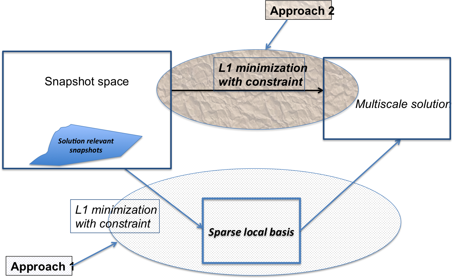
Figure 6: Illustration of the approaches.

9 Space-time GMsFEM

Many multiscale processes vary over multiple space and time scales. In many applications, the heterogeneities change due to the time can be significant and it needs to be taken into account in reduced-order models. Some well-known approaches for handling separable spatial and temporal scales are homogenization techniques [55, 63, 65, 40]. In these methods, one solves local problems in space and time. We remind a well-known case of the parabolic equation

$$\begin{split}{\partial u/\partial t}-\text{div}(\kappa(x,t)\nabla u)=f,\end{split}$$ (35)

subject to smooth initial and boundary conditions. The homogenized equation has the same form as (35), but with the smooth coefficients $\kappa^{*}(x,t)$. One can compute the coefficients using the solutions of local space-time parabolic equations in the periodic cell. This localization is possible thanks to the scale separation. One can extend this homogenization procedure to numerical homogenization type methods [61, 41], where one solves the local parabolic equations in each coarse block.

Previous approaches within GMsFEM focused on constructing multiscale spaces and relevant ingredients in space only. The extension of the GMsFEM to space-time heterogeneous problems requires a modification of the space only problems because of (1) the parabolic nature of cell solutions, (2) extra degrees of freedom associated with space-time cells, and (3) local boundary conditions in space-time cells. In the approach that we are going to discuss, we construct snapshot spaces in space-time local domains. We construct the snapshot solutions by solving local problems. We can construct a complete snapshot space by taking all possible boundary conditions; however, this can lead to very high computational cost. For this reason, we use randomized boundary conditions for local snapshot vectors. Computing multiscale basis functions employs local spectral problems in space-time domain.

We consider the parabolic differential equation (35) in a space-time domain $\Omega\times(0,T)$ and assume $u=0$ on $\partial\Omega\times(0,T)$ and $u(x,0)=\beta(x)$ in $\Omega$. The proposed method follows the space-time finite element framework, where the time dependent multiscale basis functions are constructed on the coarse grid. Therefore, compared with the time independent basis structure, it gives a more efficient numerical solver for the parabolic problem in complicated media.

We would like to compute the solution $u_{H}$ in the whole time interval $(0,T)$. In fact, if we assume the solution space $V_{H,\text{off}}^{(0,T)}$ is a direct sum of the spaces only containing the functions defined on one single coarse time interval $(T_{n-1},T_{n})$, we can decompose the problem into a sequence of problems and find the solution $u_{H}$ in each time interval sequentially. The coarse space will be constructed in each time interval and $V_{H,\text{off}}^{(0,T)}=\oplus_{n=1}^{N}V_{H,\text{off}}^{(T_{n-1},T_{n})}$, where $V_{H,\text{off}}^{(T_{n-1},T_{n})}$ only contains the functions having zero values in the time interval $(0,T)$ except $(T_{n-1},T_{n})$, namely $\forall v\in V_{H,\text{off}}^{(T_{n-1},T_{n})},$ $v(\cdot,t)=0\text{ for }t\in(0,T)\backslash(T_{n-1},T_{n})$.

The coarse-grid equation consists of finding $u_{H}^{(n)}\in V_{H,\text{off}}^{(T_{n-1},T_{n})}$ (where $V_{H,\text{off}}^{(T_{n-1},T_{n})}$ will be defined later) satisfying

$$\int_{T_{n-1}}^{T_{n}}\int_{\Omega}\cfrac{\partial u_{H}^{(n)}}{\partial t}v+\int_{T_{n-1}}^{T_{n}}\int_{\Omega}\kappa\nabla u_{H}^{(n)}\cdot\nabla v+\int_{\Omega}u_{H}^{(n)}(x,T_{n-1}^{+})v(x,T_{n-1}^{+})=\int_{T_{n-1}}^{T_{n}}\int_{\Omega}fv+\int_{\Omega}g_{H}^{(n)}(x)v(x,T_{n-1}^{+}),$$

for all $v\in V_{H,\text{off}}^{(T_{n-1},T_{n})}$, where $g_{H}^{(n)}(\cdot)=\{u_{H}^{(n-1)}(\cdot,T_{n-1}^{-})\text{ for }n\geq 1;\beta(\cdot)\text{ for }n=0\}$, and $F(\alpha^{+})$ and $F(\alpha^{-})$ denote the right hand and left hand limits of $F$ at $\alpha$ respectively. Then, the solution $u_{H}$ of the problem in $(0,T)$ is the direct sum of all these $u_{H}^{(n)}$’s, that is $u_{H}=\oplus_{n=1}^{N}u_{H}^{(n)}$.

Next, we motivate the use of space-time multiscale basis functions by comparing it to space multiscale basis functions. In particular, we discuss the savings in the reduced models when space-time multiscale basis functions are used compared to space multiscale basis functions. We denote $\{t_{n1},\cdot\cdot\cdot,t_{np}\}$ as the $p$ fine time steps in $(T_{n-1},T_{n})$. When we construct space-time multiscale basis functions, the solution can be represented as $u_{H}^{(n)}=\sum_{l,i}c_{l,i}\psi_{l}^{\omega_{i}}(x,t)$ in the interval $(T_{n-1},T_{n})$. In this case, the number of coefficients $c_{l,i}$ is related to the size of the reduced system in space-time interval. On the other hand, if we use only space multiscale basis functions, we need to construct these multiscale basis functions at each fine time instant $t_{nj}$, denoted by $\psi_{l}^{\omega_{i}}(x,t_{nj})$. The solution $u_{H}$ spanned by these basis functions will have a much larger dimension because each time instant is represented by multiscale basis functions. Thus, performing space-time multiscale model reduction can provide a substantial CPU savings.

9.1 Construction of offline basis functions

9.1.1 Snapshot space

Let $\omega$ be a given coarse neighborhood in space. We omit the coarse node index to simplify the notations. The construction of the offline basis functions on coarse time interval $(T_{n-1},T_{n})$ starts with a snapshot space $V_{H,\text{snap}}^{\omega}$ (or $V_{H,\text{snap}}^{\omega,(T_{n-1},T_{n})}$). We also omit the coarse time index $n$ to simplify the notations. The snapshot space $V_{H,\text{snap}}^{\omega}$ is a set of functions defined on $\omega$ and contains all or most necessary components of the fine-scale solution restricted to $\omega$. A spectral problem is then solved in the snapshot space to extract the dominant modes in the snapshot space. These dominant modes are the offline basis functions and the resulting reduced space is called the offline space. There are two choices of $V_{H,\text{snap}}^{\omega}$ that are commonly used.

The first choice is to use all possible fine-grid functions in $\omega\times(T_{n-1},T_{n})$. This snapshot space provides an accurate approximation for the solution space; however, this snapshot space can be very large. The second choice for the snapshot spaces consists of solving local problems for all possible boundary conditions, which we present here. As before, we denote by $\omega^{+}$ the oversampled space region of $\omega\subset\omega^{+}$, defined by adding several fine- or coarse-grid layers around $\omega$. Also, we define $(T_{n-1}^{*},T_{n})$ as the left-side oversampled time region for $(T_{n-1},T_{n})$. In the following, we generate inexpensive snapshots using random boundary conditions on the oversampled space-time region $\omega^{+}\times(T_{n-1}^{*},T_{n})$. That is for each fine boundary node on $\partial\left(\omega^{+}\times(T_{n-1}^{*},T_{n})\right)$, we solve a small number of local problems imposed with random boundary conditions

$$\begin{split}\partial\psi_{j}^{+,\omega}/\partial t-\text{div}(\kappa(x,t)\nabla\psi_{j}^{+,\omega})=0\ \ \text{in}\ \omega^{+}\times(T_{n-1}^{*},T_{n}),\ \ \psi_{j}^{+,\omega}(x,t)=r_{l}\ \ \text{on}\ \ \partial\left(\omega^{+}\times(T_{n-1}^{*},T_{n})\right),\end{split}$$

where $r_{l}$ are independent identically distributed (i.i.d.) standard Gaussian random vectors on the fine-grid nodes of the boundaries $t=T_{n-1}^{*}$ and on $\partial\omega^{+}\times(T_{n-1}^{*},T_{n})$.

Then the local snapshot space on $\omega^{+}\times(T_{n-1}^{*},T_{n})$ is

$$V_{H,\text{snap}}^{+,\omega}=\text{span}\{\psi_{j}^{+,\omega}(x,t)|j=1,\cdot\cdot\cdot,l^{\omega}+p_{\text{bf}}^{\omega}\},$$

where $l^{\omega}$ is the number of local offline basis we want to construct in $\omega$ and $p_{\text{bf}}^{\omega}$ is the buffer number. Later on, we use the same buffer number for all $\omega$’s and simply use the notation $p_{\text{bf}}$. In the following sections, if we specify one special coarse neighborhood $\omega_{i}$, we use the notation $l_{i}$ to denote the number of local offline basis. With these snapshots, we follow the procedure in the following subsection to generate offline basis functions by using an auxiliary spectral decomposition.

9.1.2 Offline space

To obtain the offline basis functions, we need to perform a space reduction by appropriate spectral problems. Motivated by a convergence analysis, we adopt the following spectral problem on $\omega^{+}\times(T_{n-1},T_{n})$. Find $(\phi,\lambda)\in V_{H,\text{snap}}^{+,\omega}\times\mathbb{R}$ such that

$$A_{n}(\phi,v)=\lambda S_{n}(\phi,v),\quad\forall v\in V_{\text{snap}}^{\omega^{+}},$$ (36)

where the bilinear operators $A_{n}(\phi,v)$ and $S_{n}(\phi,v)$ are defined by

$$\begin{split}A_{n}(\phi,v)=\frac{1}{2}\left(\int_{\omega^{+}}\phi(x,T_{n})v(x,T_{n})+\int_{\omega^{+}}\phi(x,T_{n-1})v(x,T_{n-1})\right)+\int_{T_{n-1}}^{T_{n}}\int_{\omega^{+}}\kappa(x,t)\nabla\phi\cdot\nabla v,\\ S_{n}(\phi,v)=\int_{\omega_{+}}\phi(x,T_{n-1})v(x,T_{n-1})+\int_{T_{n-1}}^{T_{n}}\int_{\omega^{+}}\widetilde{\kappa}^{+}(x,t)\phi v,\end{split}$$ (37)

where the weight function $\widetilde{\kappa}^{+}(x,t)$ is defined by $\widetilde{\kappa}^{+}(x,t)=\kappa(x,t)\sum_{i=1}^{N_{c}}|\nabla\chi_{i}^{+}|^{2}$, $\{\chi_{i}^{+}\}_{i=1}^{N_{c}}$ is a partition of unity associated with the oversampled coarse neighborhoods $\{\omega_{i}^{+}\}_{i=1}^{N_{c}}$ and satisfies $|\nabla\chi_{i}^{+}|\geq|\nabla\chi_{i}|$ on $\omega_{i}$, where $\chi_{i}$ is the standard multiscale basis function for the coarse node $x_{i}$, $-\text{div}(\kappa(x,T_{n-1})\nabla\chi_{i})=0$, in $K$, $\chi_{i}=g_{i}$ on $\partial K$, for all $K\in\omega_{i}$, where $g_{i}$ is linear on each edge of $\partial K$.

We arrange the eigenvalues $\{\lambda_{j}^{\omega}|j=1,2,\cdot\cdot\cdot\,L_{\omega}+p_{\text{bf}}^{\omega}\}$ from (36) in the ascending order, and select the first $L_{\omega}$ eigenfunctions, which are corresponding to the first $L_{\omega}$ ordered eigenvalues, and then we can obtain the dominant modes $\psi_{j}^{\omega}(x,t)$ on the target region $\omega\times(T_{n-1},T_{n})$ by restricting $\psi_{j}^{+,\omega}(x,t)$ onto $\omega\times(T_{n-1},T_{n})$. Finally, the offline basis functions on $\omega\times(T_{n-1},T_{n})$ are defined by $\phi_{j}^{\omega}(x,t)=\chi^{\omega}\psi_{j}^{\omega}(x,t)$, where $\chi^{\omega}$ is the standard multiscale basis function for a generic coarse neighborhood $\omega$. This product gives conforming basis functions (Discontinuous Galerkin discretizations can also be used). We also define the local offline space on $\omega\times(T_{n-1},T_{n})$ as

$$V_{H,\text{off}}^{\omega}=\text{span}\{\phi_{j}^{\omega}(x,t)|j=1,\cdot\cdot\cdot,l^{\omega}\}.$$

Note that one can take $V_{H,\text{off}}^{(T_{n-1},T_{n})}$ in the coarse-grid equation as $V_{H,\text{off}}^{(T_{n-1},T_{n})}=\text{span}\{\phi_{j}^{\omega_{i}}(x,t)|1\leq i\leq N_{c},1\leq j\leq l_{i}\}$.

9.2 Numerical result

We start with a high-contrast permeability field shown in Figure 4, which is translated uniformly in $x_{2}$ direction after every other fine time step. The total translation is $10$% of the global domain. The number of local offline basis that will be used in each $\omega_{i}$, is denoted by $l_{i}$, and the buffer number $p_{\text{bf}}$ needs to be chosen in advance since they determine how many local snapshots are used. Then, we can construct the lower dimensional offline space by performing space reduction on the snapshot space. In the experiments, we use the same buffer number and the same number of local offline basis for all coarse neighborhood $\omega_{i}$’s. Our numerical experiments show that the error does not change beyond $p_{\text{bf}}=4$. In our numerical simulations, we take $p_{\text{bf}}=8$ and vary $l_{i}$. The errors are displayed in Table 5. These are $L^{2}$ and energy errors. We observe that with a fixed buffer number, the relative errors are decreasing as using more offline basis. We can also observe that the values $1/\Lambda_{*}$’s and energy errors are correlated as predict our theory [19].

$L_{i}$	$dim(V_{\text{off}})$	$L^{2}([0,T],\Omega)$	energy
2	162	23.05%	87.86%
6	486	7.86%	43.29%
10	810	5.93%	35.23%
14	1134	3.43%	25.66%
18	1458	1.57%	17.42%
22	1782	0.88%	12.89%

Table 5: Relative errors using different $l_{i}$’s.

10 GMsFEM in perforated domains

One important class of multiscale problems consists in perforated domains. In these problems, differential equations are formulated in perforated domains. These domains can be considered to be the outside of inclusions or connected bodies of various sizes. Due to the variable sizes and geometries of these perforations, solutions to these problems have multiscale features. One solution approach involves posing the problem in a domain without perforations but with a very high contrast penalty term representing the domain heterogeneities ([45]). However, the void space can be a small portion of the whole domain and, thus, it is computationally expensive to enlarge the domain substantially.

The main difference in developing multiscale methods for problems in perforated domains is the complexity of the domains and that many portions of the domain are excluded in the computational domain. This poses a challenging task. For typical upscaling and numerical homogenization (e.g., [66, 48]), the macroscopic equations do not contain perforations and one computes the effective properties.

Several multiscale methods have been developed for problems in perforated domains. The use of GMsFEM for solving multiscale problems in perforated domains is motivated by recent works [59, 56, 48]. Using snapshot spaces is essential in problems with perforations, because the snapshots contain necessary geometry information. In the snapshot space, we perform local spectral decomposition to identify multiscale basis functions. In this section, we show an example for Stokes equations and refer to [26] for more discussions and extensions to other problems.

10.1 Problem setting

In this section, we present the underlying problem as stated in [20] and the corresponding fine-scale and coarse-scale discretization. Let $\Omega\subset\mathbb{R}^{d}$ ($d=2,3$) be a bounded domain covered by inactive cells (for Stokes flow and Darcy flow) or active cells (for elasticity problem) $\mathcal{B}^{\varepsilon}$. We will consider $d=2$ case, though the results can be extended to $d>2$. We use the superscript $\varepsilon$ to denote quantities related to perforated domains. The active cells are where the underlying problem is solved, while inactive cells are the rest of the region. Suppose the distance between inactive cells (or active cells) is of order $\varepsilon$. Define $\Omega^{\varepsilon}:=\Omega\backslash\mathcal{B}^{\varepsilon}$. See Figure 7 (left) for an illustration of the perforated domain. We consider the following problem defined in a perforated domain $\Omega^{\varepsilon}$

$$\mathcal{L}^{\varepsilon}(w)=f\ \text{in}\ \ \Omega^{\varepsilon},\ \ w=0\text{ or }\frac{\partial w}{\partial n}=0\text{ on }\partial\Omega^{\varepsilon}\cap\partial\mathcal{B}^{\varepsilon},$$ (38)

$w=g$ on $\partial\Omega\cap\partial\Omega^{\varepsilon}$, where $\mathcal{L}^{\varepsilon}$ denotes a linear differential operator, $n$ is the unit outward normal to the boundary, $f$ and $g$ denote given functions with sufficient regularity. We will focus on the Dirichlet problem, namely, $w=0$ in (38).

Denote by ${V}(\Omega^{\varepsilon})$ the appropriate solution space, and ${V}_{0}(\Omega^{\varepsilon})=\{v\in{V}(\Omega^{\varepsilon}),v=0\text{ on }\partial\Omega^{\varepsilon}\}$. The variational formulation of (38) is to find $w\in{V}(\Omega^{\varepsilon})$ such that

$${\left\langle\mathcal{L}^{\varepsilon}(w),v\right\rangle}_{\Omega^{\varepsilon}}=(f,v)_{\Omega^{\varepsilon}}\qquad\text{for all }v\in V_{0}(\Omega^{\varepsilon}),$$

where ${\left\langle\cdot,\cdot\right\rangle}_{\Omega^{\varepsilon}}$ denotes a specific inner product over $\Omega^{\varepsilon}$ for either scalar functions or vector functions and and $(f,v)_{\Omega^{\varepsilon}}$ is the $L^{2}$ inner product. Some specific examples for the above abstract notations are given below.

Laplace: For the Laplace operator with homogeneous Dirichlet boundary conditions on $\partial\Omega^{\varepsilon}$, we have $\mathcal{L}^{\varepsilon}(u)=-\Delta u$, and ${V}(\Omega^{\varepsilon})=H^{1}_{0}(\Omega^{\varepsilon})$, ${\left\langle\mathcal{L}^{\varepsilon}(u),v\right\rangle}_{\Omega^{\varepsilon}}=(\nabla u,\nabla v)_{\Omega^{\varepsilon}}$.

Elasticity: For the elasticity operator with a homogeneous Dirichlet boundary condition on $\partial\Omega^{\varepsilon}$, we assume the medium is isotropic. Let ${u}\in(H^{1}(\Omega^{\varepsilon}))^{2}$ be the displacement field. The strain tensor ${\mbox{$\boldsymbol{\varepsilon}$}}({u})\in(L^{2}(\Omega^{\varepsilon}))^{2\times 2}$ is defined by ${\mbox{$\boldsymbol{\varepsilon}$}}({u})=\frac{1}{2}(\nabla{u}+\nabla{u}^{T})$. Thus, the stress tensor ${\sigma}({u})\in(L^{2}(\Omega^{\varepsilon}))^{2\times 2}$ relates to the strain tensor ${\mbox{$\boldsymbol{\varepsilon}$}}({u})$ such that ${\sigma}(u)=2\mu{\mbox{$\boldsymbol{\varepsilon}$}}+\xi\nabla\cdot{u}\,{I}$, where $\xi>0$ and $\mu>0$ are the Lamé coefficients. We have $\mathcal{L}^{\varepsilon}(u)=-\nabla\cdot{\sigma}$, where ${V}(\Omega^{\varepsilon})=(H^{1}_{0}(\Omega^{\varepsilon}))^{2}$ and ${\left\langle\mathcal{L}^{\varepsilon}(u),v\right\rangle}_{\Omega^{\varepsilon}}=2\mu(\mbox{$\boldsymbol{\varepsilon}$}(u),\mbox{$\boldsymbol{\varepsilon}$}(v))_{\Omega^{\varepsilon}}+\xi(\nabla\cdot u,\nabla\cdot v)_{\Omega^{\varepsilon}}$.

Stokes: For Stokes equations, we have

$$\mathcal{L}^{\varepsilon}(u\;,p)=(\nabla p-\Delta{u},\nabla\cdot{u})^{T},$$ (39)

where $\mu$ is the viscosity, $p$ is the fluid pressure, $u$ represents the velocity, ${V}(\Omega^{\varepsilon})=(H^{1}_{0}(\Omega^{\varepsilon}))^{2}\times L^{2}_{0}(\Omega^{\varepsilon})$, and

$${\left\langle\mathcal{L}^{\varepsilon}(u\;,p),(v\;,q)\right\rangle}_{\Omega^{\varepsilon}}=\begin{pmatrix}(\nabla u,\nabla v)_{\Omega^{\varepsilon}}&-(\nabla\cdot v,p)_{\Omega^{\varepsilon}}\\ (\nabla\cdot u,q)_{\Omega^{\varepsilon}}&0\end{pmatrix}.$$

We recall that $L^{2}_{0}(\Omega^{\varepsilon})$ contains functions in $L^{2}(\Omega^{\varepsilon})$ with zero average in $\Omega^{\varepsilon}$. We will illustrate our ideas and results using the Stokes equations.

For the numerical approximation of the above problems, we first introduce the notations of fine and coarse grids pertinent to perforated domains. It follows similar constructions as before with the exception of domain geometries, which can intersect the boundaries of coarse regions. Let $\mathcal{T}_{H}$ be a coarse-grid partition of the domain $\Omega^{\varepsilon}$ with mesh size $H$. Notice that, the edges of the coarse elements do not necessarily have straight edges because of the perforations (see Figure 7, left). By conducting a conforming refinement of the coarse mesh $\mathcal{T}^{H}$, we can obtain a fine mesh $\mathcal{T}^{h}$ of $\Omega^{\varepsilon}$ with mesh size $h$. Typically, we assume that $0<h\ll H<1$, and that the fine-scale mesh $\mathcal{T}_{h}$ is sufficiently fine to fully resolve the small-scale information of the domain, and $\mathcal{T}_{H}$ is a coarse mesh containing many fine-scale features. Let $N_{v}$ and $N_{e}$ be the number of nodes and edges in coarse grid respectively. We denote by $\{x_{i}|1\leq i\leq N_{c}\}$ the set of coarse nodes, and $\{E_{j}|1\leq j\leq N_{e}\}$ the set of coarse edges. We define a coarse neighborhood $\omega_{i}^{\varepsilon}$ for each coarse node $x_{i}$ by $\omega_{i}^{\varepsilon}=\cup\{K_{j}^{\varepsilon}\in\mathcal{T}^{H};\leavevmode\nobreak\ \leavevmode\nobreak\ x_{i}\in\bar{K_{j}^{\varepsilon}}\}$, which is the union of all coarse elements having the node $x_{i}$. For the Stokes problem, additionally, we define a coarse neighborhood $\omega_{m}^{\varepsilon}$ for each coarse edge $E_{m}$ by

$$\omega_{m}^{\varepsilon}=\cup\{K_{j}^{\varepsilon}\in\mathcal{T}^{H};\leavevmode\nobreak\ \leavevmode\nobreak\ E_{m}\in\bar{K_{j}^{\varepsilon}}\},$$ (40)

which is the union of all coarse elements having the edge $E_{m}$. We let $V_{h}$ be the fine scale space for velocity $u$ and $Q_{h}$ be the fine scale space for the pressure $p$. One can choose $V_{h}$ to be piecewise quadratic and $Q_{h}$ to be piecewise constant with respect to the fine mesh $\mathcal{T}^{h}$.

We will then obtain the fine-scale solution $(u,p)\in V_{h}\times Q_{h}$ for the Stokes system by solving the following variational problem

$${\left\langle\mathcal{L}^{\varepsilon}(u,p),(v,q)\right\rangle}_{\Omega^{\varepsilon}}=((f,0),(v,q))_{\Omega^{\varepsilon}},\qquad\text{for all }(v,q)\in V_{h}\times Q_{h}.$$ (41)

These solutions are used as reference solutions to test the performance of the schemes.

10.2 The construction of offline basis functions

In this section, we describe the construction of offline basis for the Stokes problem in perforated domains. We refer to [16] for online basis construction and the analysis, as well as GMsFEM for the elliptic equation and the elasticity equations in perforated domains.

10.2.1 Snapshot space

To compute snapshot functions, we solve the following problem on the coarse neighborhood $\omega_{i}^{\varepsilon}$: find $(u^{i}_{l},p^{i}_{l})$ (on a fine grid) such that

$$\begin{split}\int_{\omega_{i}^{\varepsilon}}\nabla u^{i}_{l}:\nabla v-\int_{\omega_{i}^{\varepsilon}}p^{i}_{l}\text{div}(v)=0,\ \forall v\in V^{i}_{h,0},\ \ \int_{\omega_{i}^{\varepsilon}}q\text{div}(u^{i}_{l})=\int_{\omega_{i}^{\varepsilon}}cq,\ \forall q\in Q^{i}_{h},\end{split}$$ (42)

with boundary conditions $u^{i}_{l}=(0,0),\text{ on }\partial\mathcal{B}^{\varepsilon}$, $u^{i}_{l}=(\delta^{h}_{l},0)\text{ or }(0,\delta^{h}_{l}),\text{ on }\partial\omega_{i}^{\varepsilon}\backslash\partial\mathcal{B}^{\varepsilon}$. Here, we write $\omega_{i}^{\varepsilon}\backslash\partial\mathcal{B}^{\varepsilon}=\cup_{l=1}^{S_{i}}e_{l}$, where $e_{l}$ are the fine-grid edges and $S_{i}$ is the number of these fine grid edges on $\omega_{i}^{\varepsilon}\backslash\partial\mathcal{B}^{\varepsilon}$. Moreover, $\delta^{h}_{l}$ is a fine-scale delta function such that it has value $1$ on $e_{l}$ and value $0$ on other fine-grid edges. In (42), we define $V_{h}^{i}$ and $Q_{h}^{i}$ as the restrictions of the fine grid space in $\omega_{i}^{\varepsilon}$ and $V_{h,0}^{i}\subset V_{h}^{i}$ are functions that vanish on $\partial\omega_{i}^{\varepsilon}$. We remark that we choose the constant $c$ in (42) by compatibility condition, $c=\frac{1}{|\omega_{i}^{\varepsilon}|}\int_{\partial\omega_{i}^{\varepsilon}/\partial\mathcal{B}^{\varepsilon}}u^{i}_{l}\cdot n_{i}\,ds$. We emphasize that, for the Stokes problem, we will solve (42) in both node-based coarse neighborhoods and edge-based coarse neighborhoods (40). Collecting the solutions of the local problems generates the snapshot space, $\psi_{l}^{\omega_{i}^{\epsilon}}=u^{i}_{l}$ in $\omega_{i}^{\varepsilon}$:

$$V_{H,\text{snap}}^{\omega_{i}^{\epsilon}}=\{\psi_{l}^{\omega_{i}^{\epsilon}}:1\leq l\leq 2S_{i},\,1\leq i\leq(N_{e}+N_{v})\}.$$

One can reduce the cost of solving local problems by using the randomization techniques [9].

10.2.2 Offline Space

We perform a space reduction in the snapshot space through using a local spectral problem in $\omega_{i}^{\varepsilon}$. We consider the following local eigenvalue problem in the snapshot space

$$A^{\omega_{i}^{\epsilon}}{\Psi}_{k}^{\omega_{i}^{\epsilon}}=\lambda_{k}^{\omega_{i}^{\epsilon}}S^{\omega_{i}^{\epsilon}}{\Psi}_{k}^{\omega_{i}^{\epsilon}},$$ (43)

where $(A^{\omega_{i}^{\epsilon}})_{mn}=a_{i}(\psi_{m}^{\omega_{i}^{\varepsilon}},\psi_{n}^{\omega_{i}^{\varepsilon}})$, $(S^{\omega_{i}^{\varepsilon}})_{mn}=s_{i}(\psi_{m}^{\omega_{i}^{\varepsilon}},\psi_{n}^{\omega_{i}^{\varepsilon}})$ and $a_{i}(u,v)=\int_{\omega_{i}^{\varepsilon}}\nabla u:\nabla v$, $s_{i}(u,v)=\int_{\omega_{i}^{\varepsilon}}|\nabla\chi_{i}|^{2}u\cdot v$ with $\chi_{i}$ specified below. Note that we solve the above spectral problem in the local snapshot space corresponding to the neighborhood domain $\omega_{i}^{\varepsilon}$. We arrange the eigenvalues in an increasing order, choosing the first $l_{i}$ eigenvalues and taking the corresponding eigenvectors ${\Psi}_{k}^{\omega_{i}^{\epsilon}}$, for $k=1,2,...,l_{i}$, to form the basis functions, i.e., $\widetilde{{\Phi}}_{k}^{\omega_{i}^{\epsilon}}=\sum_{j}\Psi_{kj}^{\omega_{i}^{\epsilon}}\psi_{j}^{\omega_{i}^{\epsilon}}$, where $\Psi_{kj}^{\omega_{i}^{\epsilon}}$ are the coordinates of the vector ${\Psi}_{k}^{\omega_{i}^{\epsilon}}$. Then we define

$$\widetilde{V}^{\omega_{i}^{\varepsilon}}_{H,\text{off}}=\text{span}\{\widetilde{{\Phi}}_{k}^{\omega_{i}^{\epsilon}},\leavevmode\nobreak\ \leavevmode\nobreak\ k=1,2,...,l_{i}\}.$$

For constructing the conforming offline space, we multiply the functions $\widetilde{{\Phi}}_{k}^{\omega_{i}^{\epsilon}}=(\widetilde{\Phi}_{x_{1},k}^{\omega_{i}^{\epsilon}},\widetilde{\Phi}_{x_{2},k}^{\omega_{i}^{\epsilon}})$ by a partition of unity function $\chi_{i}$. Note that discontinuous Galerkin methods will eliminate the need for $\chi_{i}$. We remark that we define the partition of unity functions $\{\chi_{i}\}$ with respect to the coarse nodes and the mid-points of coarse edges. One can choose $\{\chi_{i}\}$ to be the standard multiscale finite element basis. However, upon multiplying by partition of unity functions, the resulting basis functions no longer have constant divergence, which affects the scheme’s stability. Moreover, the multiplication by partition of unity functions may not honor the perforation boundary conditions as discussed before. To resolve the problem with the divergence, for each $\widetilde{{\Phi}}_{k}^{\omega_{i}^{\epsilon}}$ we find two functions ${\Phi}_{1,k}^{\omega_{i}^{\epsilon}}$ and ${\Phi}_{2,k}^{\omega_{i}^{\epsilon}}$ (these are vector functions) that solve two local optimization problems in every coarse-grid element $K^{i}_{j}\subset\omega_{i}^{\varepsilon}$:

$$\min{\left\|\nabla{\Phi}_{1,k}^{\omega_{i}^{\epsilon}}\right\|_{L^{2}(K^{i}_{j})}}\text{\leavevmode\nobreak\ \leavevmode\nobreak\ such that\leavevmode\nobreak\ \leavevmode\nobreak\ }\text{div}({\Phi}_{1,k}^{\omega_{i}^{\epsilon}})=\frac{1}{|K^{i}_{j}|}\int_{\partial K^{i}_{j}}(\chi_{i}\widetilde{\Phi}_{x_{1},k}^{\omega_{i}^{\epsilon}},0)\cdot n_{ij}\,ds\quad\text{in }K^{i}_{j}$$ (44)

with $n_{ij}$ the outward normal vector to $\partial K^{i}_{j}$ and the boundary condition ${\Phi}_{1,k}^{\omega_{i}^{\epsilon}}=(\chi_{i}\widetilde{\Phi}_{x_{1},k}^{\omega_{i}^{\epsilon}},0),\text{ on }\partial K^{i}_{j}$; and

$$\min{\left\|\nabla{\Phi}_{2,k}^{\omega_{i}^{\epsilon}}\right\|_{L^{2}(K^{i}_{j})}}\text{\leavevmode\nobreak\ \leavevmode\nobreak\ such that\leavevmode\nobreak\ \leavevmode\nobreak\ }\text{div}({\Phi}_{2,k}^{\omega_{i}^{\epsilon}})=\frac{1}{|K^{i}_{j}|}\int_{\partial K^{i}_{j}}(0,\chi_{i}\widetilde{\Phi}_{x_{2},k}^{\omega_{i}^{\epsilon}})\cdot n_{ij}\,ds\quad\text{in }K^{i}_{j},$$ (45)

with the boundary condition ${\Phi}_{2,k}^{\omega_{i}^{\epsilon}}=(0,\chi_{i}\widetilde{\Phi}_{x_{2},k}^{\omega_{i}^{\epsilon}}),\text{ on }\partial K^{i}_{j}$.

Combining them, we obtain the global offline space:

$$V_{H,\text{off}}=\text{span}\{{\Phi}_{1,k}^{\omega_{i}^{\epsilon}}\text{ and }{\Phi}_{2,k}^{\omega_{i}^{\epsilon}}:\quad 1\leq i\leq(N_{e}+N_{v})\text{ and }1\leq k\leq l_{i}\}.$$

Using a single index notation, we can write $V_{H,\text{off}}=\text{span}\{{\Phi}^{\text{off}}_{i}\}_{i=1}^{N_{u}}$, where $N_{u}=\sum_{i=1}^{N_{e}+N_{v}}l_{i}$. We will use this as an approximation space for the velocity. For coarse approximation of the pressure, we will take $Q_{H,\text{off}}$ to be the space of piecewise constant functions on the coarse mesh. Note that for many applications, the size of the coarse problem can be substantially small compared to the fine-scale problem. For example, for problems with scale separation, we can only use 1-2 basis functions. Once multiscale basis functions are constructed, the global coarse-grid problem can be solved on the coarse grid with pre-computed multiscale basis functions.

10.2.3 Numerical results

We present a numerical result for Stokes equations in $\Omega=[0,1]\times[0,1]$. We consider a perforated domain as illustrated in Figure 7, where the perforated regions $\mathcal{B}^{\varepsilon}$ are circular. We coarsely discretize the computational domain using uniform triangulation, where the coarse mesh size $H=\frac{1}{5}$ for Stokes problem. Note that our approach does not impose any geometry restriction on coarse meshes. Furthermore, we use nonuniform triangulation inside each coarse triangular element to obtain a finer discretization.

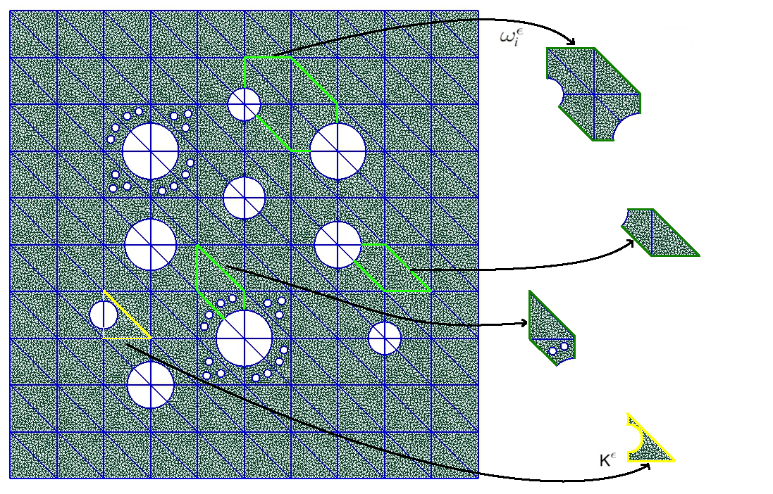
Figure 7: Heterogeneous perforated medium and the description of coarse and fine meshes.

We consider the Stokes operator with zero velocity $u=(0,0)$ on $\partial\Omega^{\varepsilon}\cap\partial\mathcal{B}^{\varepsilon}$ and ${\partial u\over\partial n}=(0,0)$ on $\partial\Omega$. For the fine-scale approximation of the Stokes problem, we use $P^{2}$-elements for velocity and piecewise constants for pressure. The $x_{1}$-component of the velocity solution is shown in Figure 8. We present the offline solution with one basis function and three basis functions. We observe that the offline velocity solution with one basis function (DOF=1082) is not able to capture the solution accurately. The $L^{2}$-error is $10.1$%. If we use three multiscale basis functions per coarse element (DOF=2846), we obtain a more accurate solution, the $L^{2}$-error is only $1.02$%. These results show that one needs a systematic and rigorous approach for enriching coarse-grid spaces in order to obtain accurate solutions using only a small number of basis functions.

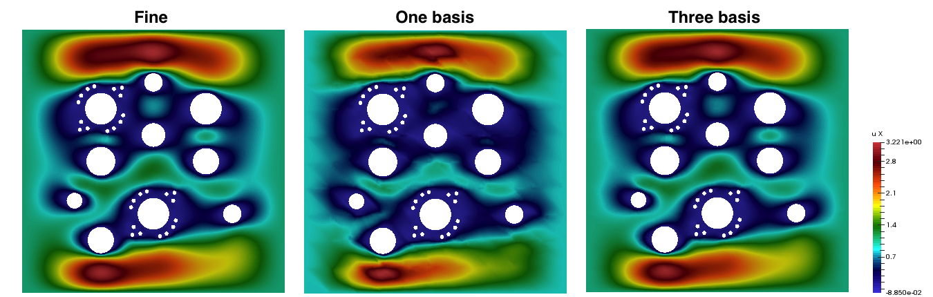
Figure 8: Stokes problem. Fine-scale and multiscale solutions for velocity $u_{1}$ in perforated domain (Figure 7). Left: fine-scale solution, $DOF=171688$. Middle: multiscale solutions using 1 multiscale basis function for the velocity ($L_{2}$ error is $10.1$%). Right: multiscale solutions with 3 multiscale basis function for the velocity ($L_{2}$ error is $1.02$%).

11 Selected Applications

Previously, we discussed the main concept of the GMsFEM and some important ingredients. The GMsFEM can be used in various applications. Below, we discuss a few applications.

11.1 Two-phase flow

We present simulation results for two-phase flow and transport problems. We consider the two-phase flow problem with zero Neumann boundary condition

$$\begin{split}-\eta(S)\kappa\nabla p={v}\mbox{ in }\Omega,\ \text{div}\,{v}=f\mbox{ in }\Omega,\ v\cdot n=0\mbox{ on }\partial\Omega,\end{split}$$ (46)

where $\eta(S)=\frac{\kappa_{rw}(S)}{\mu_{w}}+\frac{\kappa_{ro}(S)}{\mu_{o}}$ and $\kappa_{rw}(S)=S^{2}$, $\kappa_{ro}(S)=(1-S)^{2}$, $\mu_{w}=1$, $\mu_{o}=5$. The saturation equation is given by

$$S_{t}+v\cdot\nabla F(S)=r,$$

where $F(S)=\frac{\kappa_{rw}(S)/\mu_{w}}{\kappa_{rw}(S)/\mu_{w}+\kappa_{ro}(S)/\mu_{o}}$. The above flow equation (46) is solved by the mixed GMsFEM, and the saturation equation is solved on the fine grid by the finite volume method. In our simulations, we take $f$ to be zero except for the top-left and bottom-right fine-grid elements, where $f$ takes the values of $1$ and $-1$, respectively. Moreover, we set the initial value of $S$ to be zero. For the source $r$, we also take it as zero except for the top-left fine element where $r=1$.

For the simulations of two-phase flow, the mixed GMsFEM is used for the flow equations. The multiscale basis functions are computed at time zero using the unit mobility, i.e., $\eta=1$. These multiscale basis function for the velocity field is used without any modification to compute the fine-scale velocity field. The fine-scale velocity field is further used to update the saturation file. We note that each time the flow equation is solved on a coarse grid, which provides a substantial computational saving. We present the numerical results for the saturation in Figure 9 for the permeability field shown in Figure 4. As we observe from this figure that with three basis functions, we obtain very good agreement ($L^{2}$ error is $1.8$%).

(a) Fine-grid solution

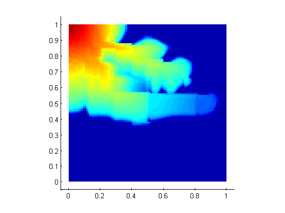
(b) Relative $L^{2}$ error = 1.8%

Figure 9: Saturation solution obtained by using $v_{o}$ ($10\times 10$ coarse grid, 3 basis per coarse edge)

11.2 Flow in fractured media

In this section, we briefly discuss the application of the GMsFEM to flows in fractured media, in particular, the application to shale gas transport in fractured media. We remark that the study of flows in fractured media has a long history (see, e.g., [57, 46]). We study nonlinear gas transport in fractured media (cf., [2])

$$a_{z}(c){\partial c\over\partial t}=\text{div}(b_{z}(c,x)\nabla c),$$ (47)

where $z=m,f$ with $m$ referring to the matrix phase and $f$ referring to the fracture phase. The fractures have “zero” thickness and are represented on a fine-scale variational formulation as edge elements. More precisely, the domain $\Omega$ can be represented by $\Omega=\Omega_{m}\oplus_{i}\,d_{i}\Omega_{f,i}$. Here, $d_{i}$ is the aperture of the $i$ th fracture and $i$ is the index of the fractures (see Figure 10). Then, the fine-scale equations have the form

$$\begin{split}\int_{\Omega_{m}}a_{m}(c){\partial c\over\partial t}v+\sum\limits_{i}d_{i}\int_{\Omega_{f,i}}a_{f}(c){\partial c\over\partial t}v++\int_{\Omega_{m}}b_{m}(c,x)\nabla c\cdot\nabla v+\sum\limits_{i}d_{i}\int_{\Omega_{f,i}}b_{m}(c,x)\nabla c\cdot\nabla v=0.\end{split}$$ (48)

In our numerical simulations, we solve the above problem using the GMsFEM framework for some specific parameter values that are specified below. We note that the fractures are modeled within snapshot space via harmonic extensions as we discussed above (see [1] for more details). In the method, the basis functions are constructed using the steady state with $b_{z}=1$ in (47) and taking into account the fracture distribution. The problem (47) is solved by using implicit discretization and by linearizing $c$ at the previous time step.

We use following parameters: $a_{{m}}(c)=\phi+(1-\phi){\partial F}/{\partial c}$; $b_{m}(c,x)=\phi D+(1-\phi)D_{s}{\partial F}/{\partial c}+\phi{\kappa}RTc/\mu$; $a_{f}(c)=\phi_{f}$; $b_{f}(c,x)={\kappa_{f}}RTc/\mu$; $D=510^{-7}[m^{2}/s]$, $\phi=0.04$, $T=413[K]$, $\mu=2\cdot 10^{-5}[kg/(m\,s)]$ and for fractures $k_{f}=10^{-12}[m^{2}]$, $\phi_{f}=0.001$. As for permeability $\kappa$, we use constant $\kappa=10^{-18}[m^{2}]$. $p=RTc$, $p_{c}=10^{9}[Pa]$, $p_{1}=1.8\cdot 10^{9}[Pa]$, $\alpha=0.5$ and $\mathcal{M}=0.5$. For the sorbed gas, we use Langmuir model $F(c)=c_{\mu s}\frac{s}{(1+sc)^{2}}$, where $s=0.26\cdot 10^{-3}$ and $c_{\mu s}=0.25\cdot 10^{-5}[mol/m^{3}]$. We present the numerical results in Figure 10. In the left figure, we depict the fracture distributions, and then, show the fine-scale and the coarse-scale solution. We observe that with only $4$ basis functions, we obtain a good agreement between the fine-scale and multiscale solution ($L^{2}$ error $0.34$%, $H^{1}$ error $4.69$%).

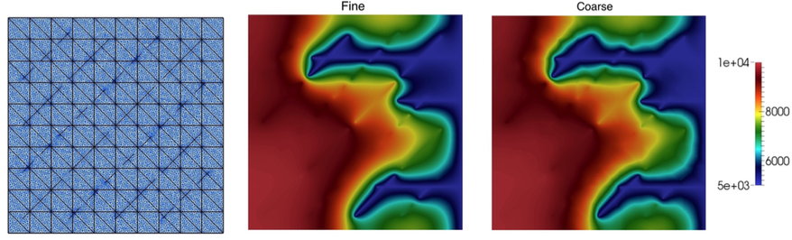
Figure 10: Left: the fracture distributions. Middle: the fine-scale solution. Right: the coarse-grid solution.

11.3 Other applications

We have demonstrated two applications of the GMsFEM. The GMsFEM can be used for other complex multiscale problems. For example, in [13], we have applied the GMsFEM for elastic wave propagation in fractured media. We have also used the GMsFEM for acoustic wave propagation [22]. The GMsFEM can also be effectively used in inverse problem, where the forward problem is solved many times. In [38], we apply the GMsFEM in uncertainty quantification in inverse problems.

12 Discussions

In this paper, we give an overview of multiscale finite element methods and discuss their generalizations. Due to page limitations, we do not present a comprehensive overview of multiscale methods and mention only some important aspects of the GMsFEM as a tool for performing adaptive multiscale model reduction. The application of the method to nonlinear problems is not discussed in the paper. We refer to ([17]) for the application to nonlinear problems, where we consider nonlinear eigenvalue problems, hybridization, and nonlinear interpolation ideas to efficiently solve these problems.

The proposed local reduced-order models can be used in performing global model reduction. The GMsFEM can be employed to construct the snapshots for the global model reduction methods. In this case, using reduced representation of the global snapshots, we can perform POD or another model reduction for the global modes. Moreover, we can use adaptively local approaches to update the global snapshots when online computations are needed. These global-local approaches can be effective in many applications [3].

Optimal multiscale basis functions can be obtained using the oversampling techniques, optimization, and singular value decomposition [51]. In this paper, we focus on a general adaptive strategy that can be easily adapted for various applications and discretization, as demonstrated. One can use the ideas of optimized multiscale basis functions as in [51] in the proposed framework.

The stochastic multiscale problems are challenging due to additional degrees of freedom due to randomness. For stochastic problems, one can use multiscale finite element framework with Monte Carlo techniques or separation of variables. A promising approach for solving multiscale stochastic problems is to use data driven stochastic method concepts as shown in [69].

Multiscale framework proposed in the paper can also be employed for the stabilization. For example, in [7], the authors use the GMsFEM to stabilize the convection-dominated problems by constructing multiscale test spaces.

Finally, we would like to remark that the proposed methods are well suited for the parallel computation, in particular, the task of multiscale basis computations is embarrassingly parallel. Our numerical results (using up to $1000$ processors) on 3D perforated problems show that one can achieve almost perfect scaling in the parallel computations.

Acknowledgements. TYH’s research was in part supported by DOE Grant DE-FG02-06ER257, and NSF Grant No. DMS-1318377, DMS-1159138. EC’s research was in part supported by Hong Kong RGC General Research Fund Project No. 400813.

References

- [1] IY Akkutlu, Yalchin Efendiev, and Maria Vasilyeva. Multiscale model reduction for shale gas transport in fractured media. arXiv preprint arXiv:1507.00113, 2015.
- [2] Y Akkutlu, Y Efendiev, and V Savatarova. Multiscale asymptotic analysis of gas transport in shale matrix. Transport in Porous Media, pages 1–26, 2015.
- [3] M Alotaibi, VM Calo, Y Efendiev, JC Galvis, and M Ghommem. Global–local nonlinear model reduction for flows in heterogeneous porous media. Computer Methods in Applied Mechanics and Engineering, 292:122–137, 2015.
- [4] T. Arbogast, G. Pencheva, M.F. Wheeler, and I. Yotov. A multiscale mortar mixed finite element method. SIAM J. Multiscale Modeling and Simulation, 6(1):319–346, 2007.
- [5] M. Barrault, Y. Maday, N.C. Nguyen, and A.T. Patera. An ‘Empirical Interpolation’ Method: Application to Efficient Reduced-Basis Discretization of Partial Differential Equations. C.R. Acad. Sci. Paris, Ser. I, 339:667–672, 2004.
- [6] S. Boyaval, C. LeBris, T. Lelièvre, Y. Maday, N. Nguyen, and A. Patera. Reduced basis techniques for stochastic problems. Archives of Computational Methods in Engineering, 17:435–454, 2010.
- [7] V. Calo, E. Chung, Y. Efendiev, and W. T. Leung. Multiscale stabilization for convection-dominated diffusion in heterogeneous media. arXiv preprint arXiv:1509.06833. to appear in CMAME.
- [8] VM Calo, Y Efendiev, J Galvis, and M Ghommem. Multiscale empirical interpolation for solving nonlinear PDEs. Journal of Computational Physics, 278:204–220, 2014.
- [9] VM Calo, Y Efendiev, J Galvis, and G Li. Randomized oversampling for generalized multiscale finite element methods. http://arxiv.org/pdf/1409.7114.pdf. to appear in SIAM MMS.
- [10] VM Calo, Y Efendiev, and JC Galvis. A note on variational multiscale methods for high-contrast heterogeneous porous media flows with rough source terms. ADWR, 34(9):1177–1185, 2011.
- [11] E. Candès et al. Compressive sampling. Proceedings of the ICM, 3:1433–1452, 2006.
- [12] S. Chaturantabut and D. C. Sorensen. Application of POD and DEIM to dimension reduction of nonlinear miscible viscous fingering in porous media. Mathematical and Computer Modeling of Dynamical Systems, 17:337–353, 2011.
- [13] E. Chung, Y. Efendiev, R. Gibson, and M. Vasilyeva. A generalized multiscale finite element method for elastic wave propagation in fractured media. 2015. submitted.
- [14] E. Chung, Y. Efendiev, T. W. Leung, and G. Li. Sparse generalized multiscale finite element methods and their applications. arXiv preprint arXiv:1506.08509. to appear in IJ Multiscale Computational Engineering.
- [15] E. Chung, Y. Efendiev, and W. T. Leung. An adaptive generalized multiscale discontinuous galerkin method (GMsDGM) for high-contrast flow problems. arXiv preprint arXiv:1409.3474, 2014.
- [16] E. Chung, Y. Efendiev, W.T. Leung, M. Vasilyeva, and Y. Wang. Adaptive online generalized multiscale finite element method for multiscale problems in perforated domain. submitted.
- [17] E. Chung, Y. Efendiev, K. Shi, and S. Ye. A multiscale model reduction method for nonlinear monotone elliptic equations in heterogeneous media. submitted.
- [18] E. Chung, Y. Efendiev, and T. Wing. Generalized multiscale finite element methods with energy minimizing oversampling. submitted.
- [19] E. Chung, Y. Efendiev, T. Wing, and S. Ye. Generalized multiscale finite element methods for space-time heterogeneous parabolic equations. submitted.
- [20] E. T. Chung, Y. Efendiev, G. Li, and M. Vasilyeva. Generalized multiscale finite element method for problems in perforated heterogeneous domains. Applicable Analysis, 255:1–15, 2015.
- [21] ET Chung, Y Efendiev, and CS Lee. Mixed generalized multiscale finite element methods and applications. Multiscale Modeling & Simulation, 13(1):338–366, 2015.
- [22] E.T. Chung, Y. Efendiev, and W.T. Leung. Generalized multiscale finite element method for wave propagation in heterogeneous media. to appear in SIAM MMS.
- [23] ET Chung, Y Efendiev, and WT Leung. Residual-driven online generalized multiscale finite element methods. To appear in J. Comput. Phys.
- [24] ET Chung, Y Efendiev, and WT Leung. An online generalized multiscale discontinuous Galerkin method (GMsDGM) for flows in heterogeneous media. arXiv preprint arXiv:1504.04417, 2015.
- [25] ET Chung, Y Efendiev, and G Li. An adaptive GMsFEM for high-contrast flow problems. Journal of Computational Physics, 273:54–76, 2014.
- [26] ET Chung, Y Efendiev, G Li, and M Vasilyeva. Generalized multiscale finite element methods for problems in perforated heterogeneous domains. Applicable Analysis, to appear, 2015.
- [27] W. Dorfler. A convergent adaptive algorithm for poisson’s equation. SINUM, 33:1106 – 1124, 1996.
- [28] M. Drohmann, B. Haasdonk, and M. Ohlberger. Reduced basis approximation for nonlinear parametrized evolution equations based on empirical operator interpolation. SIAM J. Sci. Comput., 34(2):A937–A969, 2012.
- [29] W. E and B. Engquist. Heterogeneous multiscale methods. Comm. Math. Sci., 1(1):87–132, 2003.
- [30] W.T. Leung E. Chung and S. Pollock. Goal-oriented adaptivity for GMsFEM. Journal of Computational and Applied Mathematics, 296:625–637, 2016.
- [31] Y. Efendiev and J. Galvis. A domain decomposition preconditioner for multiscale high-contrast problems. In Y. Huang, R. Kornhuber, O. Widlund, and J. Xu, editors, Domain Decomposition Methods in Science and Engineering XIX, volume 78 of Lect. Notes in Comput. Science and Eng., pages 189–196. Springer-Verlag, 2011.
- [32] Y. Efendiev, J. Galvis, and T. Hou. Generalized multiscale finite element methods. Journal of Computational Physics, 251:116–135, 2013.
- [33] Y Efendiev, J Galvis, R Lazarov, M Moon, and M Sarkis. Generalized multiscale finite element method. Symmetric interior penalty coupling. Journal of Computational Physics, 255:1–15, 2013.
- [34] Y. Efendiev, J. Galvis, R. Lazarov, and J. Willems. Robust domain decomposition preconditioners for abstract symmetric positive definite bilinear forms. ESIAM : M2AN, 46:1175–1199, 2012.
- [35] Y. Efendiev, J. Galvis, G. Li, and M. Presho. Generalized multiscale finite element methods. Oversampling strategies. International Journal for Multiscale Computational Engineering, accepted, 2013.
- [36] Y. Efendiev, V. Ginting, T. Hou, and R. Ewing. Accurate multiscale finite element methods for two-phase flow simulations. Journal of Computational Physics, 220:155–174, 2006.
- [37] Y. Efendiev and T. Hou. Multiscale Finite Element Methods: Theory and Applications. Springer, 2009.
- [38] Y. Efendiev, B. Jin, M. Presho, and X. Tan. Multilevel markov chain monte carlo method for high-contrast single-phase flow problems. Communications in Computational Physics, 17(01):259–286, 2015.
- [39] Y. Efendiev, R. Lazarov, M. Moon, and K. Shi. A spectral multiscale hybridizable discontinuous Galerkin method for second order elliptic problems. Computer Methods in Applied Mechanics and Engineering, 292:243–256, 2015.
- [40] Y Efendiev, A Pankov, et al. Homogenization of nonlinear random parabolic operators. Advances in Differential Equations, 10(11):1235–1260, 2005.
- [41] Jacob Fish. Practical multiscaling. John Wiley & Sons, 2013.
- [42] J. Galvis and Y. Efendiev. Domain decomposition preconditioners for multiscale flows in high contrast media. Reduced dimensional coarse spaces. SIAM J. Multiscale Modeling and Simulation, 8:1621–1644, 2010.
- [43] J Galvis, G Li, and K Shi. A generalized multiscale finite element method for the Brinkman equation. Journal of Computational and Applied Mathematics, 280:294–309, 2015.
- [44] J. Galvis and J. Wei. Ensemble level multiscale finite element and preconditioner for channelized systems and applications. Journal of Computational and Applied Mathematics, 255:456–467, 2014.
- [45] M. Griebel and M. Klitz. Homogenization and numerical simulation of flow in geometries with textile microstructures. Multiscale Modeling & Simulation, 8(4):1439–1460, 2010.
- [46] H. Hajibeygi, D. Kavounis, and P. Jenny. A hierarchical fracture model for the iterative multiscale finite volume method. Journal of Computational Physics, 230(4):8729–8743, 2011.
- [47] Patrick Henning, Axel Malqvist, and Daniel Peterseim. A localized orthogonal decomposition method for semi-linear elliptic problems. arXiv preprint arXiv:1211.3551, 2012.
- [48] Patrick Henning and Mario Ohlberger. The heterogeneous multiscale finite element method for elliptic homogenization problems in perforated domains. Numerische Mathematik, 113(4):601–629, 2009.
- [49] M. Hinze and S. Volkwein. POD surrogate models for nonlinear dynamical systems: error estimates and suboptimal control. volume 45 of Lecture Notes in CSE, pages 261–306. 2005.
- [50] T. Hou and X.H. Wu. A multiscale finite element method for elliptic problems in composite materials and porous media. J. Comput. Phys., 134:169–189, 1997.
- [51] Thomas Y Hou and Pengfei Liu. Optimal local multi-scale basis functions for linear elliptic equations with rough coefficient. arXiv preprint arXiv:1508.00346, 2015.
- [52] T.Y. Hou, X.H. Wu, and Z. Cai. Convergence of a multiscale finite element method for elliptic problems with rapidly oscillating coefficients. Math. Comp., 68:913–943, 1999.
- [53] TJR Hughes, G Feijoo, L Mazzei, and J Quincy. The variational multiscale method—a paradigm for computational mechanics. Comput. Methods Appl. Mech. Engrg., 166:3–24, 1998.
- [54] P. Jenny, S.H. Lee, and H. Tchelepi. Multi-scale finite volume method for elliptic problems in subsurface flow simulation. J. Comput. Phys., 187:47–67, 2003.
- [55] V. Jikov, S. Kozlov, and O. Oleinik. Homogenization of differential operators and integral functionals. Springer Science & Business Media, 2012.
- [56] C. Le Bris, F. Legoll, and A. Lozinski. An MsFEM type approach for perforated domains. Multiscale Modeling & Simulation, 12(3):1046–1077, 2014.
- [57] S.H. Lee, M.F. Lough, and C.L. Jensen. Hierarchical modeling of flow in naturally fractured formations with multiple length scales. Water resources research, 37(3):443–455, 2001.
- [58] Ana-Maria Matache and Christoph Schwab. Two-scale fem for homogenization problems. ESAIM: Mathematical Modelling and Numerical Analysis, 36(04):537–572, 2002.
- [59] V. Maz’ya, A. Movchan, and M. Nieves. Green Kernels and Meso-Scale Approximations in Perforated Domains. Springer-Berlin, Lecture Notes in Mathematics, 2077, 2013.
- [60] Jens M Melenk and Ivo Babuška. The partition of unity finite element method: basic theory and applications. Computer methods in applied mechanics and engineering, 139(1):289–314, 1996.
- [61] P. Ming and P. Zhang. Analysis of the heterogeneous multiscale method for parabolic homogenization problems. Mathematics of Computation, 76(257):153–177, 2007.
- [62] H. Owhadi and L. Zhang. Metric-based upscaling. Comm. Pure. Appl. Math., 60:675–723, 2007.
- [63] Aleksandr Andreevich Pankov. G-convergence and homogenization of nonlinear partial differential operators, volume 422. Springer Science & Business Media, 2013.
- [64] G Papanicolau, A Bensoussan, and J-L Lions. Asymptotic analysis for periodic structures. Elsevier, 1978.
- [65] Grigorios A Pavliotis and Andrew Stuart. Multiscale methods: averaging and homogenization. Springer Science & Business Media, 2008.
- [66] Enrique Sánchez-Palencia. Non-homogeneous media and vibration theory. In Non-homogeneous media and vibration theory, volume 127, 1980.
- [67] Hayden Schaeffer, Russel Caflisch, Cory D Hauck, and Stanley Osher. Sparse dynamics for partial differential equations. Proceedings of the National Academy of Sciences, 110(17):6634–6639, 2013.
- [68] X.H. Wu, Y. Efendiev, and T.Y. Hou. Analysis of upscaling absolute permeability. Discrete and Continuous Dynamical Systems, Series B., 2:158–204, 2002.
- [69] Zhiwen Zhang, Maolin Ci, and Thomas Y Hou. A multiscale data-driven stochastic method for elliptic pdes with random coefficients. Multiscale Modeling & Simulation, 13(1):173–204, 2015.