Gravitational bending angle of light for finite distance and the Gauss-Bonnet theorem

Abstract

We discuss a possible extension of calculations of the bending angle of light in a static, spherically symmetric and asymptotically flat spacetime to a non-asymptotically flat case. We examine a relation between the bending angle of light and the Gauss-Bonnet theorem by using the optical metric. A correspondence between the deflection angle of light and the surface integral of the Gaussian curvature may allow us to take account of the finite distance from a lens object to a light source and a receiver. Using this relation, we propose a method for calculating the bending angle of light for such cases. Finally, this method is applied to two examples of the non-asymptotically flat spacetimes to suggest finite-distance corrections: Kottler (Schwarzschild-de Sitter) solution to the Einstein equation and an exact solution in Weyl conformal gravity.

I Introduction

The gravitational bending of light by mass led to the first experimental confirmations of the theory of general relativity. In modern astronomy and cosmology, the gravitational lensing is widely used as one of the important tools for probing extrasolar planets, dark matter and dark energy.

The light bending is also of theoretical importance, especially for studying a null structure of a spacetime. A rigorous form of the bending angle plays an important role in understanding properly a strong gravitational field Frittelli ; VE2000 ; Virbhadra ; VNC ; VE2002 ; VK2008 ; ERT ; Perlick . For example, strong gravitational lensing in a Schwarzschild black hole was considered by Frittelli, Kling and Newman Frittelli , by Virbhadra and Ellis VE2000 and more comprehensively by Virbhadra Virbhadra ; Virbhadra, Narasimha and Chitre VNC studied distinctive lensing features of naked singularities. Virbhadra and Ellis VE2002 and Virbhadra and Keeton VK2008 later described the strong gravitational lensing by naked singularities; DeAndrea and Alexander DA discussed the lensing by naked singularities to test the cosmic censorship hypothesis; Eiroa, Romero and Torres ERT treated Reissner-Nordström black hole lensing; Perlick Perlick discussed the lensing by a Barriola-Vilenkin monopole and also that by an Ellis wormhole. Kitamura, Nakajima and Asada proposed a lens model whose gravitational potential declines as $1/r^{n}$ Kitamura in order to study the gravitational lensing by exotic matter (or energy) Tsukamoto ; Izumi ; Kitamura2014 ; Nakajima2014 that might follow a non-standard equation of state. See Tsukamoto et. al. (2015) Tsukamoto2014 for its possible connection to the Tangherlini solution to the higher-dimensional Einstein equation.

Some recent papers give the expressions for the deflection of light for the Kottler (often called Schwarzschild-de Sitter) spacetime Kottler ; Lake ; RI ; Park ; Sereno ; Bhadra ; Simpson ; AK and for the spherical, static and vacuum exact solution in Weyl conformal gravity MK ; Riegert ; Edery ; Sultana ; Cattani . However, their results are not in agreement with each other and hence they are controversial. The apparent inconsistency among the previous works might be caused, because the spacetimes are not asymptotically flat and their methods are no longer appropriate for treating such a non-asymptotically flat spacetime. In the non-asymptotically flat spacetime, we can never assume that the source of light is located at infinite distance from a gravitational lens object. The main purpose of this paper is to discuss a possible extension of calculations of the bending angle of light in a static, spherically symmetric and asymptotically flat spacetime, particularly in order to find finite-distance corrections.

For this purpose, we shall examine a relation between the bending angle of light and the Gauss-Bonnet theorem in differential geometry. In this sense, the present paper may discuss a possible extension of Gibbons and Werner (2008) GW2008 . They considered two different domains: one (say, $\cal{D}$) bounded by two light rays, to exhibit the connection between topology and multiple images; and the other (say, $\cal{D}^{\prime}$) bounded by one light ray and a non-geodesic circular arc, to compute the asymptotic deflection angle. They suggested that the asymptotic deflection angle of light can be written as the surface integral of the Gaussian curvature over the domain $\cal D^{\prime}$. They did integrate only for the asymptotic case, for which they assumed the observer and source are in the asymptotically Euclidean region. Namely, the angles at the location of the observer and source are defined only in Euclidean space GW2008 .

Throughout this paper, we use the unit of $G=c=1$. In the following, the observer may be called the receiver in order to avoid a confusion between $r_{O}$ and $r_{0}$ by using $r_{R}$.

II Light Propagation, optical metric and Gauss-Bonnet theorem

II.1 Static and spherically symmetric spacetime

We consider a static and spherically symmetric (SSS) spacetime. The SSS spacetime can be described as

$$ds^{2} = g_{\mu\nu}dx^{\mu}dx^{\nu}$$ (1)

$$= g_{tt}(r)dt^{2}+g_{rr}(r)dr^{2}+r^{2}d\Omega^{2},$$

where the origin of the spatial coordinates is chosen as the location of a lens object, $\mu$ and $\nu$ run from $0$ to $3$, and $d\Omega^{2}\equiv d\theta^{2}+\sin^{2}\theta d\phi^{2}$. By introducing two functions as $A(r)\equiv-g_{tt}$ and $B(r)\equiv g_{rr}$, Eq. (1) is rewritten as

$$ds^{2} = -A(r)dt^{2}+B(r)dr^{2}+r^{2}d\Omega^{2}.$$ (2)

II.2 Optical metric

Light rays satisfy the null condition as $ds^{2}=0$, which is rearranged as, via Eq. (2),

$$dt^{2} = \gamma_{ij}dx^{i}dx^{j}$$ (3)

$$= \frac{B(r)}{A(r)}dr^{2}+\frac{r^{2}}{A(r)}d\Omega^{2},$$

where $i$ and $j$ denote $1$, $2$ and $3$, and $\gamma_{ij}$ is often called the optical metric gamma . The optical metric defines a three-dimensional Riemannian space (denoted as $M^{\mbox{opt}}$), in which the light ray is expressed as a spatial curve.

For the spherically symmetric spacetime, without the loss of generality, we can choose the photon orbital plane as the equatorial plane ($\theta=\pi/2$). The two-dimensional coordinates on the equatorial plane are denoted as $x^{I}$ ($I=1,2$), where $I$ may mean $r$, $\phi$ particularly in the polar coordinates. The nonvanishing components of the optical metric are

$$\gamma_{rr} = \frac{B(r)}{A(r)},$$ (4)

$$\gamma_{\phi\phi} = \frac{r^{2}}{A(r)}.$$ (5)

Let us suppose the tangent vector field along the light ray. The unit tangential vector along the light ray in $M^{\mbox{opt}}$ can be defined as

$$K^{I}\equiv\frac{dx^{I}}{dt}.$$ (6)

This is a spatial vector. Note that $K^{I}$ is defined in terms of $\gamma_{IJ}$ but not $g_{IJ}$, because we consider light rays.

II.3 Impact parameter

In the SSS spacetime, there are two constants of motion for a massless particle such as a photon. They are the specific energy and the specific angular momentum as

$$E = A(r)\frac{dt}{d\lambda},$$ (7)

$$L = r^{2}\frac{d\phi}{d\lambda},$$ (8)

where $\lambda$ denotes the affine parameter along the light ray. As usual, we define the impact parameter of the light ray as

$$b \equiv \frac{L}{E}$$ (9)

$$= \frac{r^{2}}{A(r)}\frac{d\phi}{dt}.$$

In terms of the impact parameter and the metric components at the position of the massless particle, the components of $K^{I}$ can be expressed as

$$(K^{r},K^{\phi})=\frac{bA(r)}{r^{2}}\left(\frac{dr}{d\phi},1\right).$$ (10)

Here, the unity of the vector $K^{I}$ leads to the orbit equation as

$$\left(\frac{dr}{d\phi}\right)^{2}+\frac{r^{2}}{B(r)}=\frac{r^{4}}{b^{2}A(r)B(r)}.$$ (11)

This can be also derived directly from $ds^{2}=0$.

Is it safe for us to call what is defined as $b$ the impact parameter of light? Let us briefly mention this. If there were no lens objects, then the spacetime would be Minkowskian, namely $A(r)=1$ and $B(r)=1$ in the polar coordinates, and $b$ would thus equal to the closest distance according to Eq. (11). Therefore, $b$ can be safely called the impact parameter of the orbit.

II.4 Angles

We can define the dyad as

$$e^{I}_{\mbox{rad}} = \left(\frac{1}{\sqrt{\gamma_{rr}}},0\right),$$ (12)

$$e^{I}_{\mbox{ang}} = \left(0,\frac{1}{\sqrt{\gamma_{\phi\phi}}}\right),$$ (13)

which correspond to the unit vector along the radial direction from the center of the lens object and that along the angular direction, respectively.

Let $\Psi$ denote the angle of the light ray measured from the radial direction. It can be defined by

$$\cos\Psi\equiv\gamma_{IJ}e^{I}_{\mbox{rad}}K^{J},$$ (14)

where we used that $e^{I}_{\mbox{rad}}$ and $K^{J}$ are unit vectors. This expression is rewritten more explicitly as

$$\cos\Psi = \gamma_{rr}e^{r}_{\mbox{rad}}K^{r}$$ (15)

$$= \frac{\sqrt{\gamma_{rr}}bA(r)}{r^{2}}\frac{dr}{d\phi}.$$

This leads to

$$\sin\Psi=\frac{b\sqrt{A(r)}}{r},$$ (16)

where we used Eq. (11).

When we want to obtain $\Psi$ at a point in $M^{\mbox{opt}}$, $\sin\Psi$ by Eq. (16) is more convenient than $\cos\Psi$ by Eq. (15), because $b\sqrt{A(r)}/r$ can be immediately calculated but $\cos\Psi$ includes $dr/d\phi$ that requires a more lengthy calculation.

Let $\Psi_{R}$ and $\Psi_{S}$ denote the angles that are measured at the receiver position and the source position, respectively. Moreover, let $\phi_{R}$ and $\phi_{S}$ denote the longitudes of the receiver and the source, respectively Memo-Scalars . Let $\phi_{RS}\equiv\phi_{R}-\phi_{S}$ denote the coordinate separation angle between the receiver and source. From the three angles $\Psi_{R}$, $\Psi_{S}$ and $\phi_{RS}$, let us define

$$\alpha\equiv\Psi_{R}-\Psi_{S}+\phi_{RS}.$$ (17)

This is a key equation in the present paper.

Every two points among the three points of the receiver (R), the source (S) and the lens center (L) are connected by the geodesics in the space $M^{\mbox{opt}}$. Hence, the three points in a non-Euclidean space constitute an embedded triangle (denoted as ${}^{R}\bigtriangledown^{S}_{L}$). The above definition of $\alpha$ depends on the three angles. Therefore, we might be dissatisfied with the definition of $\alpha$, because the comparison of the scalars at spatially distinct points such as $R$ and $S$ is quite unclear and even questionable. Let us examine whether $\alpha$ is well-defined.

First, we focus on the triangle ${}^{R}\bigtriangledown^{S}_{L}$. Let $\Psi_{L}$ denote the the interior angle at the vertex $L$. The angle $\Psi_{S}$ is the exterior angle at the vertex $S$ and $\Psi_{R}$ is the opposite angle of the interior angle at the vertex $R$ by definition. Let us define

$$\alpha_{\Psi}\equiv\Psi_{R}-\Psi_{S}+\Psi_{L}.$$ (18)

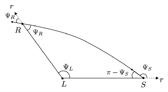
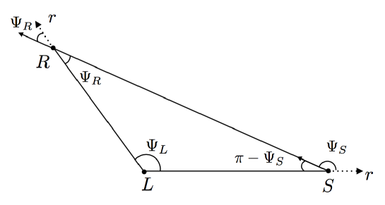
Figure 1: Top: Triangle embedded in a curved space. $\alpha_{\Psi}$ does not always vanish. Bottom: Triangle in Euclidean space. It follows that $\alpha_{\Psi}=0$.

Note that $\Psi_{R}$ is the same as the interior angle at $R$. See Figure 1. Consequently, Eq. (18) is rearranged as

$$\alpha_{\Psi}=\sum_{a=1}^{3}\varepsilon_{a}-\pi,$$ (19)

where $\varepsilon_{a}$ $(a=1,2$ and $3$) mean the interior angles in the triangle ${}^{R}\bigtriangledown^{S}_{L}$.

If the space $M^{\mbox{opt}}$ is flat, it follows that $\alpha_{\Psi}=0$. Hence, this might allow us to interpret $\alpha_{\Psi}$ as a measure of the deviation from Euclidean space. We shall apply Gauss-Bonnet theorem to the triangle ${}^{R}\bigtriangledown^{S}_{L}$ below.

II.5 Gauss-Bonnet theorem

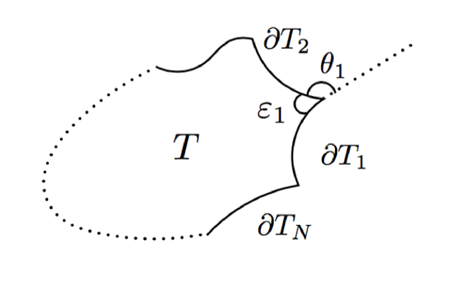
Figure 2: Schematic figure for the Gauss-Bonnet theorem.

Suppose that $T$ is a two-dimensional orientable surface with boundaries $\partial T_{a}$ ($a=1,2,\cdots,N$) that are differentiable curves (See Figure 2). Let the jump angles between the curves be $\theta_{a}$ ($a=1,2,\cdots,N$). Then, the Gauss-Bonnet theorem can be expressed as GB-theorem

$$\iint_{T}KdS+\sum_{a=1}^{N}\int_{\partial T_{a}}\kappa_{g}d\ell+\sum_{a=1}^{N}\theta_{a}=2\pi,$$ (20)

where $K$ denotes the Gaussian curvature of the surface $T$, $dS$ is the area element of the surface, $\kappa_{g}$ means the geodesic curvature of $\partial T_{a}$, and $\ell$ is the line element along the boundary. The sign of the line element is chosen such that it is compatible with the orientation of the surface.

By using the Gauss-Bonnet theorem for $N=3$ case, Eq. (19) is rewritten as

$$\alpha_{\Psi}=\iint_{{}^{R}\bigtriangledown^{S}_{L}}KdS+\int_{L}^{S}\kappa_{g}d\ell+\int_{S}^{R}\kappa_{g}d\ell+\int_{R}^{L}\kappa_{g}d\ell,$$ (21)

where we use $\varepsilon_{a}+\theta_{a}=\pi$ at each point ($a=1,\cdots,N=3$).

For our case, $\kappa_{g}=0$ along the boundary curves kappag=0 . Therefore, we obtain

$$\alpha_{\Psi}=\iint_{{}^{R}\bigtriangledown^{S}_{L}}KdS.$$ (22)

Eq. (22) shows clearly that $\alpha_{\Psi}$ is invariant in differential geometry. The definition by Eq. (18) is thus justified geometrician . The Gaussian curvature can be related with the Riemannian tensor. See e.g. Werner (2012) for this relation Werner2012 ; K-Comment .

However, it seems impossible to define $\Psi_{L}$ for a case of a black hole, because $L$ is the singularity. On the other hand, $\phi_{RS}$ seems preferred for practical calculations in order to avoid such a problem associated with $\Psi_{L}$, because $\phi_{RS}$ can be defined outside the horizon for a black hole case.

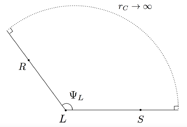
Figure 3: Embedded triangle ${}^{\infty}\bigtriangledown^{\infty}_{L}$. It consists of a circular arc segment $C_{r}$ of coordinate radius $r_{C}$ centered at the lens with taking $r_{C}\to\infty$, and two radial geodesics through either the receiver or the source. One can determine $\Psi_{L}$ at the point $L$ from this figure by using the Gauss-Bonnet theorem. See Eq. (23).

We begin by considering another embedded triangle, which consists of a circular arc segment $C_{r}$ of coordinate radius $r_{C}$ centered at the lens which intersects the radial geodesic through the receiver or the source. See Figure 3, in which we assume the asymptotically flat spacetime and a sufficiently large $r_{C}$, for which the embedded triangle is denoted by ${}^{\infty}\bigtriangledown^{\infty}_{L}$. Then, $\kappa_{g}\to 1/r_{C}$ and $d\ell\to r_{C}d\phi$ as $r_{C}\to\infty$ (See e.g. GW2008 ). Hence, we obtain $\int_{C_{r}}\kappa_{g}d\ell\to\phi_{RS}$. Applying this result to the Gauss-Bonnet theorem for ${}^{\infty}\bigtriangledown^{\infty}_{L}$ leads to

$$\Psi_{L}=\phi_{RS}+\iint_{{}^{\infty}\bigtriangledown^{\infty}_{L}}KdS.$$ (23)

By substituting Eq. (23) into $\Psi_{L}$ in $\alpha_{\Psi}$ of Eq. (22), we obtain

$$\alpha = \Psi_{R}-\Psi_{S}+\phi_{RS}$$ (24)

$$= -\iint_{{}^{\infty}_{R}\Box^{\infty}_{S}}KdS,$$

where we use Eq. (17) and ${}^{\infty}_{R}\Box^{\infty}_{S}$ denotes an oriented area of ${}^{\infty}\bigtriangledown^{\infty}_{L}$ subtracted by ${}^{R}\bigtriangledown^{S}_{L}$. Eq. (24) shows that $\alpha$ is invariant in differential geometry. Moreover, it follows that $\alpha=0$ in Euclidean space.

Both $\alpha$ and $\alpha_{\Psi}$ are geometrically invariant. The integration domain for $\alpha_{\Psi}$ includes the lens position. Therefore, $\alpha_{\Psi}$ might not be suitable for a black hole case.

On the other hand, it is likely that $\alpha$ can avoid such a problem. Furthermore, in next section, we shall see that (1) $\alpha$ by Eq. (17) recovers the known formula of the bending angle for the asymptotic receiver and source and (2) it can be done in practice to calculate $\alpha$ without encountering an infinitely large term for a non-asymptotically flat model, though the justification of $\alpha$ by Eq. (24) is currently limited within an asymptotically flat case.

III Method of calculating the bending angle of light

There are two ways of calculating $\alpha$, because Eq. (17) always agrees with Eq. (24). One method is to use Eq. (17). For this method, all we have to do is to calculate the three angles of $\Psi_{R}$, $\Psi_{S}$ and $\phi_{RS}$. The other method is to use Eq. (24), where we first calculate the Gaussian curvature $K$ by using the optical metric and next we integrate $K$ over the quadrilateral ${}^{\infty}_{R}\Box^{\infty}_{S}$. Note that the integration domain ${}^{\infty}_{R}\Box^{\infty}_{S}$, especially an expression of the geodesic curve from $S$ to $R$, is unknown a priori and hence it must be looked for, though the calculation must be straightforward but tedious. Let us suppose an asymptotic receiver and source of light in the Schwarzschild spacetime for instance. Even in this case, it is a quite elaborate task to calculate the surface integral to recover the known formula $\alpha=4M/b$. See Gibbons ans Werner (2008) GW2008 . As a result, it is likely that the first method is much easier than the second one.

III.1 Asymptotically flat case

Let us consider the case of the asymptotic flatness. Then, we can assume $A(r)\to 1$ and $B(r)\to 1$ as $r\to\infty$. As usual, we assume also that the source and receiver are located at the null infinity. Namely, we assume $r_{R}\to\infty$ and $r_{S}\to\infty$. Then, let us examine whether Eq. (17) can recover the textbook formula for the deflection angle of light. For this purpose, we assume $\Psi_{R}=0$ and $\Psi_{S}=\pi$, because we keep $b$ constant with $r_{R}\to\infty$ and $r_{S}\to\infty$.

Hence, we obtain

$$\alpha=\phi_{RS}-\pi.$$ (25)

All we have to do is to compute $\phi_{RS}$.

The orbit equation for the light ray in the SSS spacetime is in a general form as

$$\left(\frac{du}{d\phi}\right)^{2} = F(u),$$ (26)

where $u$ denotes the inverse of $r$. Please see Eq. (11) for more detail.

Integrating Eq. (26) leads to the angle $\phi_{RS}$ as

$$\phi_{RS} = 2\int_{0}^{u_{0}}\frac{du}{\sqrt{F(u)}},$$ (27)

where $u_{0}$ is the inverse of the closest approach (often denoted as $r_{0}$). Therefore, substituting this into Eq. (17) gives

$$\alpha=2\int_{0}^{u_{0}}\frac{du}{\sqrt{F(u)}}-\pi.$$ (28)

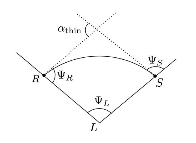
Figure 4: Thin lens approximation. In this approximation, the light ray deflects only at the lens plane. Namely, we assume that the spacetime is flat except for the location of the thin lens, so that $\Psi_{L}$ in this figure can be identified with $\phi_{RS}$. Let $\alpha_{\mbox{thin}}$ denote the deflection angle of light in the thin lens approximation. The dotted straight lines are tangential to the light ray at the receiver or at the source. For the quadrilateral in Euclidean space, $\alpha_{\mbox{thin}}=\Psi_{R}-\Psi_{S}+\phi_{RS}$, because the sum of the inner angles is $2\pi$.

This is exactly the deflection angle of light in the literature. Therefore, $\alpha$ may be interpreted as the deflection angle of light. See also Figure 4 for the thin lens approximation. One can see that $\alpha$ is likely to correspond to $\alpha_{\mbox{thin}}$, where $\alpha_{\mbox{thin}}$ denotes the deflection angle of light in the thin lens approximation.

III.2 Finite distance cases

In practice, the thin lens approximation works well for most cases in astronomy so far. This approximation is almost the same as an assumption that a light source and a receiver are nearly at the null infinity in the asymptotically flat case. To be more specific, the present paper assumes that the distance from the source to the receiver is finite because every observed stars and galaxies are located at finite distance from us (e.g., at finite redshift in cosmology) and the distance is much larger than the size of the lens. Hence, we keep $r_{R}$ and $r_{S}$ finite. Then, let $u_{R}$ and $u_{S}$ denote the inverse of $r_{R}$ and $r_{S}$, respectively. Eq. (17) becomes

$$\alpha=\int_{u_{R}}^{u_{0}}\frac{du}{\sqrt{F(u)}}+\int_{u_{S}}^{u_{0}}\frac{du}{\sqrt{F(u)}}+\Psi_{R}-\Psi_{S}.$$ (29)

Eq. (28) is thus corrected.

Eq. (17), Eq. (24) and Eq. (29) are equivalent to each other. They are different from the deflection angle that is often used (or argued) in the recent papers previous .

For the Schwarzschild spacetime, the line element becomes

$$ds^{2} = -\left(1-\frac{r_{g}}{r}\right)dt^{2}+\frac{dr^{2}}{\displaystyle 1-\frac{r_{g}}{r}}$$ (30)

$$+r^{2}(d\theta^{2}+\sin^{2}\theta d\phi^{2}).$$

Then, $F(u)$ is

$$F(u)=\frac{1}{b^{2}}-u^{2}+r_{g}u^{3}.$$ (31)

By using Eq. (16), $\Psi_{R}-\Psi_{S}$ in the Schwarzschild spacetime is expanded in a power series in $r_{g}$ as

$$\Psi_{R}^{\mbox{Sch}}-\Psi_{S}^{\mbox{Sch}} \equiv [\arcsin(bu_{R})+\arcsin(bu_{S})-\pi]$$ (32)

$$-\frac{1}{2}br_{g}\left(\frac{u_{R}^{2}}{\sqrt{1-b^{2}u_{R}^{2}}}+\frac{u_{S}^{2}}{\sqrt{1-b^{2}u_{S}^{2}}}\right)+O(br_{g}^{2}u_{S}^{3},br_{g}^{2}u_{R}^{3}).$$

It follows that $\Psi_{R}-\Psi_{S}$ for the Schwarzschild case approaches $\pi$ as $u_{S}\to 0$ and $u_{R}\to 0$.

IV Non-asymptotically flat cases

Finally, we consider a non-asymptotically flat spacetime such as the Kottler solution to the Einstein equation and an exact solution in the Weyl conformal gravity. For such cases, we cannot assume the source at the past null infinity ($r_{S}\to\infty$) nor the receiver at the future null infinity ($r_{R}\to\infty$), because $A(r)$ diverges or does not exist as $r\to\infty$. Hence, we should keep the source and the receiver to be at finite distance from the lens object. It is Eq. (29) that we can use for such a case. As mentioned already, Eq. (16) is more convenient for calculating $\Psi_{R}$ and $\Psi_{S}$ than Eq. (14), since Eq. (16) needs a local quantity but not any derivative. For the two cases, the explicit expressions are as follows.

IV.1 Kottler case

For the Kottler spacetime Kottler , the line element is

$$ds^{2} = -\left(1-\frac{r_{g}}{r}-\frac{\Lambda}{3}r^{2}\right)dt^{2}+\frac{dr^{2}}{\displaystyle 1-\frac{r_{g}}{r}-\frac{\Lambda}{3}r^{2}}$$ (33)

$$+r^{2}(d\theta^{2}+\sin^{2}\theta d\phi^{2}),$$

where $\Lambda$ denotes the cosmological constant.

By using Eq. (16), $\Psi_{R}-\Psi_{S}$ is expanded in terms of $r_{g}$ and $\Lambda$ as

$$\Psi_{R}-\Psi_{S} =\Psi^{Sch}_{R}-\Psi^{Sch}_{S}-\frac{b\Lambda}{6u_{R}\sqrt{1-b^{2}u_{R}^{2}}}-\frac{b\Lambda}{6u_{S}\sqrt{1-b^{2}u_{S}^{2}}}$$

$$+\frac{bu_{R}(-1+2b^{2}u_{R}^{2})}{8(1-b^{2}u_{R}^{2})^{3/2}}\left(r_{g}^{2}u_{R}^{2}+\frac{2r_{g}\Lambda}{3u_{R}}+\frac{\Lambda^{2}}{9u_{R}^{4}}\right)$$

$$+\frac{bu_{S}(-1+2b^{2}u_{S}^{2})}{8(1-b^{2}u_{S}^{2})^{3/2}}\left(r_{g}^{2}u_{S}^{2}+\frac{2r_{g}\Lambda}{3u_{S}}+\frac{\Lambda^{2}}{9u_{S}^{4}}\right)$$

$$+O(r_{g}^{3},r_{g}^{2}\Lambda,r_{g}\Lambda^{2},\Lambda^{3}),$$ (34)

where $\Psi_{R}^{\mbox{Sch}}-\Psi_{S}^{\mbox{Sch}}$ is a part existing in Schwarzschild spacetime. Note that the above expansion of $\Psi_{R}-\Psi_{S}$ is divergent as $u_{S}\to 0$ and $u_{R}\to 0$. This is because the spacetime is not asymptotically flat and hence it does not allow the limit of $u_{S}\to 0$ and $u_{R}\to 0$. Hence, the power series form by Eq. (34) must be used within a certain finite radius of convergence.

For the Kottler case, $F(u)$ becomes

$$F(u)=\frac{1}{b^{2}}-u^{2}+r_{g}u^{3}+\frac{\Lambda}{3}.$$ (35)

Hence, we obtain

$$\phi_{RS}= \pi-\arcsin(bu_{R})-\arcsin(bu_{S})$$

$$+\frac{r_{g}}{b}\left[\frac{1}{\sqrt{1-b^{2}u_{R}^{2}}}\left(1-\frac{1}{2}b^{2}u_{R}^{2}\right)+\frac{1}{\sqrt{1-b^{2}u_{S}^{2}}}\left(1-\frac{1}{2}b^{2}u_{S}^{2}\right)\right]$$

$$+\frac{\Lambda b^{3}}{6}\left[\frac{u_{R}}{\sqrt{1-b^{2}u_{R}^{2}}}+\frac{u_{S}}{\sqrt{1-b^{2}u_{S}^{2}}}\right]+\frac{r_{g}\Lambda b}{12}\left[\frac{2-3b^{2}u_{R}^{2}}{(1-b^{2}u_{R}^{2})^{\frac{3}{2}}}+\frac{2-3b^{2}u_{S}^{2}}{(1-b^{2}u_{S}^{2})^{\frac{3}{2}}}\right]+O(r_{g}^{2},\Lambda^{2}).$$ (36)

By using Eqs. (34) and (36), we obtain the correct deflection angle of light as

$$\alpha= \frac{r_{g}}{b}\left[\sqrt{1-b^{2}u_{R}^{2}}+\sqrt{1-b^{2}u_{S}^{2}}\right]$$

$$-\frac{\Lambda b}{6}\left[\frac{\sqrt{1-b^{2}u_{R}^{2}}}{u_{R}}+\frac{\sqrt{1-b^{2}u_{S}^{2}}}{u_{S}}\right]$$

$$+\frac{r_{g}\Lambda b}{12}\left[\frac{1}{\sqrt{1-b^{2}u_{R}^{2}}}+\frac{1}{\sqrt{1-b^{2}u_{S}^{2}}}\right]+O(r_{g}^{2},\Lambda^{2}).$$ (37)

Some terms in this expression may apparently diverge in the limit as both $bu_{R}\to 0$ and $bu_{S}\to 0$. Note that this limit has no relevance with astronomical observations in the Kottler spacetime. Therefore, the apparent divergence does not matter.

Aghili, Bolen and Bombelli have recently discussed numerically effects of a slowly varying Hubble parameter on the gravitational lensing Aghili . It is left as a future work to examine an application of the present approach to such a cosmological model with a slowly varying Hubble parameter.

IV.2 Weyl conformal gravity case

Weyl conformal gravity introduces three independent parameters (often denoted as $\beta$, $\gamma$ and $k$) into the spherical solution, for which Birkhoff’s theorem was proven in conformal gravity Riegert . The line element with the three parameters is MK

$$ds^{2} = -A(r)dt^{2}+\frac{1}{A(r)}dr^{2}+r^{2}(d\theta^{2}+\sin^{2}\theta d\phi^{2}),$$

$$A(r) = 1-3m\gamma-\frac{2m}{r}+\gamma r-kr^{2},$$ (38)

where we defined $m\equiv\beta(2-3\beta\gamma)/2$. The term with the coefficient $k$ makes the same contribution as the cosmological constant in the Kottler spacetime that has been studied above. Henceforth, we omit the $r^{2}$ term for brevity.

By using Eq. (16), $\Psi_{R}-\Psi_{S}$ is expanded in a power series in $\beta$ and $\gamma$ as

$$\Psi_{R}-\Psi_{S}\equiv \Psi_{R}^{\mbox{Sch}}-\Psi_{S}^{\mbox{Sch}}$$

$$+\frac{b\gamma}{2}\left(\frac{u_{R}}{\sqrt{1-b^{2}u^{2}_{R}}}+\frac{u_{S}}{\sqrt{1-b^{2}u^{2}_{S}}}\right)$$

$$-\frac{m\gamma}{2}\left[\frac{bu_{R}(2-b^{2}u_{R}^{2})}{(1-b^{2}u_{R}^{2})^{3/2}}+\frac{bu_{S}(2-b^{2}u_{S}^{2})}{(1-b^{2}u_{S}^{2})^{3/2}}\right]+O(m^{2},\gamma^{2}).$$ (39)

Note that this series expansion of $\Psi_{R}-\Psi_{S}$ is divergent as $u_{S}\to 0$ and $u_{R}\to 0$. This is because the non-asymptotic flatness of the spacetime does not allow the limit of $u_{S}\to 0$ and $u_{R}\to 0$. Hence, we must use Eq. (39) within its certain radius of convergence.

For the conformal gravity case with $k=0$, $F(u)$ becomes

$$F(u)=\frac{1}{b^{2}}-u^{2}+2mu^{3}+\Gamma u^{2}-\gamma u.$$ (40)

Then, $\phi_{RS}$ is obtained as

$$\phi_{RS}= [\pi-\arcsin(bu_{R})-\arcsin(bu_{S})]$$

$$+\frac{m}{b}\left(\frac{2-b^{2}u_{R}^{2}}{\sqrt{1-b^{2}u_{R}^{2}}}+\frac{2-b^{2}u_{S}^{2}}{\sqrt{1-b^{2}u_{S}^{2}}}\right)$$

$$-\frac{\gamma}{2}\left(\frac{b}{\sqrt{1-b^{2}u_{R}^{2}}}+\frac{b}{\sqrt{1-b^{2}u_{R}^{2}}}\right)$$

$$+\frac{m\gamma}{2}\left[\frac{b^{3}u_{R}^{3}}{(1-b^{2}u_{R}^{2})^{3/2}}+\frac{b^{3}u_{S}^{3}}{(1-b^{2}u_{S}^{2})^{3/2}}\right]+O(m^{2},\gamma^{2}).$$ (41)

In total, we obtain $\alpha$ for the Weyl conformal gravity case as

$$\alpha= \frac{2m}{b}\left(\sqrt{1-b^{2}u_{R}^{2}}+\sqrt{1-b^{2}u_{S}^{2}}\right)$$

$$-m\gamma\left(\frac{bu_{R}}{\sqrt{1-b^{2}u_{R}^{2}}}+\frac{bu_{S}}{\sqrt{1-b^{2}u_{S}^{2}}}\right)+O(m^{2},\gamma^{2}).$$ (42)

The terms linear in $\gamma$ cancel out in the expression for the deflection angle of light. Hence, this might correct the results in previous papers Edery ; Sultana ; Cattani that reported non-zero contributions from $\gamma$.

IV.3 Far source and receiver

Finally, let us consider an asymptotic case as $bu_{S}\ll 1$ and $bu_{R}\ll 1$, which mean that both the source and the receiver are very far from the lens object. Note that $bu_{S}\to 0$ and $bu_{R}\to 0$ might cause the divergent terms in the deflection angle. Hence, we focus on the dominant part of each term in a series expansion without taking the limit. Let us write down approximate expressions for the deflection of light.

(1) Kottler case:
It follows that the expression for $\phi_{RS}$ in the far approximation coincides with the seventh and eighth terms of Eq. (5) in Sereno , the third and fifth terms of Eq. (15) in Bhadra , and the second term of Eq. (14) in AK . However, they Sereno ; Bhadra ; AK did not consider $\Psi_{R}-\Psi_{S}$. Eq. (37) becomes

$$\alpha\sim\frac{2r_{g}}{b}-\frac{1}{6}\Lambda b\left(\frac{1}{u_{R}}+\frac{1}{u_{S}}\right)+\frac{1}{6}r_{g}\Lambda b.$$ (43)

This might give a correction to the previous results Sereno ; Bhadra ; AK . For instance, Sereno (2009) considered only $\phi_{RS}$. See previous for a more subtle case associated with Rindler and Ishak’s approach.

(2) Weyl conformal gravity case:
For the Weyl conformal gravity, the deflection angle of light in the far approximation becomes

$$\alpha \sim \frac{4m}{b}+O(m^{2},\gamma^{2}).$$ (44)

Note that $m\gamma$ parts from $\Psi_{R}-\Psi_{S}$ and from $\psi_{RS}$ cancel out. See Eqs. (39) and (41).

Before closing this section, we briefly mention another light path (Path 2 in Figure 5). The bending angle for this path is computable, if we take account of the orientation of Path 2 (See Fig. 5).

V Conclusion

In this paper, we studied a connection between the bending angle of light and the Gauss-Bonnet theorem by using the optical metric in the SSS spacetimes. A correspondence of the deflection angle of light to the surface integral of Gaussian curvature may allow us to take account of the finite distance of a light source and a receiver from a lens object.

The proposed approach of calculating the deflection angle of light by Eq. (17) was applied to two examples of the non-asymptotically flat spacetimes: Kottler solution to the Einstein equation and an exact solution in Weyl conformal gravity. For the both cases, we suggested finite-distance corrections to the deflection angle of light without encountering an infinitely large term, as a conjecture, because the justification of $\alpha$ by Eq. (24) cannot be applied to such a non-asymptotically flat case as it is. It would be interesting to examine whether or not the justification of Eq. (17) is extended to a non-asymptotically flat case. If it is not, we may find new corrections to the deflection angle of light. It would be interesting to study along this direction.

Moreover, let us suppose that the light ray passes near a relativistic compact object. For this case, the deflection angle of light may exceed $2\pi$ to procedure the relativistic images. For such a large deflection case, the orbit has the winding number $W$ that may be the unity or more. Eqs. (17) and (22) still work, because the light ray lives on a single plane in $M^{\mbox{opt}}$ Weyl-Comment . Further study along the direction of the relativistic strong lensing by using the present approach is left for future work.

We are grateful to Marcus Werner for the stimulating discussions, especially for his useful comments on the Gauss-Bonnet theorem and the earlier version of the manuscript. We wish to thank Makoto Sakaki for giving us the useful literature information on the Gauss-Bonnet theorem. We would like to thank Toshifumi Futamase, Masumi Kasai, Yuuiti Sendouda, Ryuichi Takahashi, Koji Izumi, Tomohito Suzuki and Takumi Takahashi for the useful conversations. This work was supported in part by JSPS Grant-in-Aid for Scientific Research, (Kiban C) No. 26400262 (H.A.) and in part by MEXT (Shingakujutsu) No. 15H00772 (H.A.).

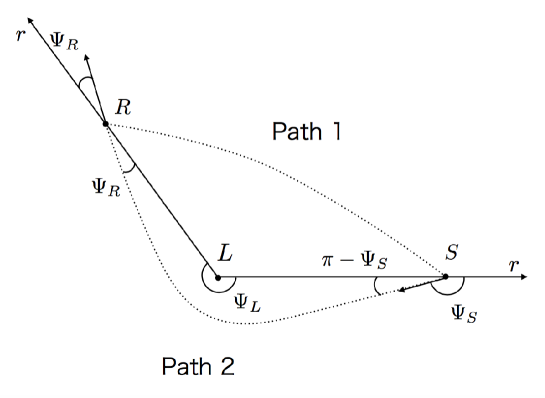
Figure 5: Two light paths. In the present paper, we focus on the path 1 in this figure, because it corresponds to the brightest lensed image and it plays a crucial role in astronomy. There is another possible path (Path 2 in this figure). The two light paths are denoted by dotted lines.

References

- (1) S. Frittelli, T. P. Kling, and E. T. Newman, Phys. Rev. D 61, 064021 (2000).
- (2) K. S. Virbhadra, and G. F. R. Ellis, Phys. Rev. D 62, 084003 (2000).
- (3) K. S. Virbhadra, Phys. Rev. D 79, 083004 (2009).
- (4) K. S. Virbhadra, D. Narasimha, and S. M. Chitre, Astron. Astrophys. 337, 1 (1998).
- (5) K. S. Virbhadra, and G. F. R. Ellis, Phys. Rev. D 65, 103004 (2002).
- (6) K. S. Virbhadra, and C. R. Keeton, Phys. Rev. D 77, 124014 (2008).
- (7) E. F. Eiroa, G. E. Romero, and D. F. Torres, Phys. Rev. D 66, 024010 (2002).
- (8) V. Perlick, Phys. Rev. D 69, 064017 (2004).
- (9) J. P. DeAndrea, and K. M. Alexander, Phys. Rev. D 89, 123012 (2014).
- (10) T. Kitamura, K. Nakajima, and H. Asada, Phys. Rev. D 87, 027501 (2013).
- (11) K. Izumi, C. Hagiwara, K. Nakajima, T. Kitamura, and H. Asada, Phys. Rev. D 88, 024049 (2013).
- (12) T. Kitamura, K. Izumi, K. Nakajima, C. Hagiwara, and H. Asada, Phys. Rev. D 89, 084020 (2014).
- (13) K. Nakajima, K. Izumi, and H. Asada, Phys. Rev. D 90, 084026 (2014).
- (14) N. Tsukamoto, and T. Harada, Phys. Rev. D 87, 024024 (2013).
- (15) N. Tsukamoto, T. Kitamura, K. Nakajima, and H. Asada, Phys. Rev. D 90, 064043 (2014).
- (16) F. Kottler, Annalen. Phys. 361, 401 (1918).
- (17) K. Lake, Phys. Rev. D 65, 087301 (2002).
- (18) W. Rindler and M. Ishak, Phys. Rev. D 76, 043006 (2007); M. Ishak and W. Rindler, Gen. Relativ. Gravit. 42, 2247 (2010).
- (19) M. Park, Phys. Rev. D 78, 023014 (2008).
- (20) M. Sereno, Phys. Rev. Lett. 102, 021301 (2009).
- (21) A. Bhadra, S. Biswas, and K. Sarkar, Phys. Rev. D 82, 063003 (2010).
- (22) F. Simpson, J. A. Peacock, and A. F. Heavens, Mon. Not. R. Astron. Soc. 402, 2009 (2010).
- (23) H. Arakida, and M. Kasai, Phys. Rev. D 85, 023006 (2012).
- (24) P. D. Mannheim and D. Kazanas, Astrophys. J. 342, 635 (1989).
- (25) M. E. Aghili, B. Bolen and L. Bombelli, ArXiv:1408.0786
- (26) R. J. Riegert, Phys. Rev. Lett. 53, 315 (1984).
- (27) A. Edery, and M. B. Paranjape, Phys. Rev. D 58, 024011 (1998).
- (28) J. Sultana, and D. Kazanas, Phys. Rev. D 81, 127502 (2010).
- (29) Carlo Cattani, Massimo Scalia, Ettore Laserra, Ivana Bochicchio, and Kamal K. Nandi, Phys. Rev. D 87, 047503 (2013).
- (30) G. W. Gibbons, M. C. Werner, Class. Quant. Grav. 25, 235009 (2008).
- (31) To be more precise, might be denoted as , since the notation as is often used for the induced metric on a hypersurface in the 3+1 formulation in the literature. However, we use for denoting the optical metric for its simplicity in this paper, because the induced metric does not appear in this paper and hence readers would not be confused.
- (32) Let us suppose two scalars. One scalar is defined at a point . The other scalar is at a very different point . The sum of and and the difference between and have no invariant meaning in general.
- (33) Fermat’s principle in a spacetime is the principle that the light path makes the arrival time stationary. It is expressed as along the light ray Perlick . In our case, hence, Eq. (3) implies that the orbit of light is a geodesic in with the optical metric .
- (34) M. P. Do Carmo, Differential Geometry of Curves and Surfaces, pages 268-269, (Prentice-Hall, New Jersey, 1976).
- (35) It is likely that mathematicians prefer to define by Eq. (22). However, it is quite elaborate in practice to perform the areal integral of Eq. (22). In order to do it, we have to find out the integration domain first, especially the domain boundary connecting the receiver and the source. This boundary is the light ray that is unknown a priori for most cases and hence the expression of the boundary can be obtained only after the orbit equation is solved.
- (36) M. C. Werner, Gen. Relativ. Grav. 44, 3047 (2012).
- (37) in our notation. See e.g. Eq. (16) in Werner(2012) Werner2012 . can diverge at for black hole cases. For such cases, it is likely that Eq. (22) requires more mathematical treatments, because the singularity at is hidden by a horizon. Further study along this mathematical direction is left for future work.
- (38) In discussing the effect of the cosmological constant on the bending of light, Rindler and Ishak have proposed a different definition of the deflection angle of light as , where the source (and also the receiver) is assumed to be at rest at the very special point that is defined as an intersection between the light ray and the curve. Note that their calculations and results, even if they were correct, can be applied only for the particular positions of the receiver and source ( and ) and hence the applicability of their argument seems very narrow. Moreover, their deflection angle (denoted as ) can be written as in the notation of the present paper. Apparently, agrees with Eq. (17) only for a particular case that is chosen by hand, such that the geometrical configuration of the lens, receiver and source can be the same as that in Rindler and Ishak. There is a significant difference, in spite of the apparent coincidence between the two definitions. Note that they use a simple spatial metric to define a covariant angle that is different from the angle in the present paper. The definition of and in the present paper is based on the optical metric that respects describing the null geodesics projected onto a spatial sector . Practically speaking, is different from by a factor in a SSS spacetime. See also Eqs. (4) and (5). Rindler and Ishak’s approach has been criticized by numerous authors (See Park ; Sereno ; Simpson ; AK ). Following the pioneering work by Lake Lake , for instance, Arakida and Kasai claimed that, even if the cosmological constant is taken into account, the deflection angle of light can be rearranged as to agree with that in Schwarzschild spacetime, if the impact parameter is replaced by a new impact parameter in order to absorb the influence of the cosmological constant AK . Arakida and Kasai continued to argue that the orbit equation in the presence of the cosmological constant becomes the same as that for the Schwarzschild case, after the impact parameter is suitably shifted. Therefore, they concluded that the deflection angles for both cases agreed with each other. However, this final step in their argument is misleading. The receiver and source can be located at the null infinity for the Schwarzschild case. On the other hand, we can never assume and for the Kottler case, because the receiver and source go across de-Sitter horizon in this limit. In other words, they should have integrated the orbit equation from a finite-distance source to a finite-distance receiver. If they had done it, they might have obtained the deflection angle with certain corrections due to the finiteness of distance. Note that their paper did not even define the deflection angle of light for finite distance nor take care of the optical metric. The observer at rest in a static slice of the spacetime may be in motion in a different slice. This is the case, for instance in the Kottler solution, where an observer at rest at the static chart can be in motion in the cosmological coordinates of the same spacetime. See e.g. Park (2008), Simpson et al. (2010) for detailed discussions on the corrections to the deflection angle of light due to different time slices Park ; Simpson .
- (39) It is likely that the nonvanishing contributions to at the linear order of and in the previous works are because they did not use the optical metric to define the angles at the receiver and the source and they employed a different definition of by following RI . In particular, does not contribute at the leading order. It might be interesting to interpret this thing by a projective equivalence GWW between the solution in the Weyl conformal gravity and another spacetime.
- (40) G. W. Gibbons, C. M. Warnick, M. C. Werner, Class. Quant. Grav. 25, 245009 (2008).