Abnormality Detection in Correlated Gaussian Molecular Nano-Networks: Design and Analysis

Siavash Ghavami and Farshad Lahouti S. Ghavami is with the Department of Electrical & Computer Engineering, University of Minnesota, USA and F. Lahouti is with the Electrical Engineering Department, California Institute of Technology, USA; E-mail: sghavami@umn.edu,lahouti@caltech.edu.
Abstract

A nano abnormality detection scheme (NADS) in molecular nano-networks is studied. This is motivated by the fact that early detection of diseases such as cancer play a crucial role in their successful treatment. The proposed NADS is in fact a two-tier network of sensor nano-machines (SNMs) in the first tier and a data-gathering node (DGN) at the sink. The SNMs detect the presence of competitor cells (abnormality) by variations in input and/or parameters of a nano-communications channel (NCC). The noise of SNMs as their nature suggest is considered correlated in time and space and herein assumed additive Gaussian. In the second step, the SNMs transmit micro-scale messages over a noisy micro communications channel (MCC) to the DGN, where a decision is made upon fusing the received signals. We find an optimum design of detectors for each of the NADS tiers based on the end-to-end NADS performance. The detection performance of each SNM is analyzed by setting up a generalized likelihood ratio test. Next, taking into account the effect of the MCC, the overall performance of the NADS is analyzed in terms of probabilities of misdetection and false alarm. In addition, computationally efficient expressions to quantify the NADS performance is derived by providing respectively an approximation and an upper bound for the probabilities of misdetection and false alarm. This in turn enables formulating a design problem, where the optimized concentration of SNMs in a sample is obtained for a high probability of detection and a limited probability of false alarm. The results indicate that otherwise ignoring the spatial and temporal correlation of SNM noise in the analysis, leads to an NADS that noticeably underperforms in operations.

Index Terms:
Abnormality detection, Molecular communication, Mathematical modeling, Correlation.

I Introduction

Cancer is a leading cause of death in the world and accounts for about 13% of all death per annum [1]. In addition, it incurs serious disability and emotional challenges to the people and heavily affects them financially [2]. There have been many advances by significant technological innovations in the treatment of cancer. However, success is still a distant goal in this direction. Indeed, research in early detection and diagnostics of cancer and their associated enabling technologies are of extraordinary importance.

It is believed that the overall behavior of cancer is determined with genes expressions and/or proteins. In fact, proteomic data and collective functions of proteins are known to directly set the cell function. Hence, modeling and analysis of genomic and proteomic data using micro array and mass spectrometry technologies have found various applications in cancer studies [3]. In [4], an interesting review of technologies for nano-scale cancer bio-molecular detection using proteomic and genomic approaches is presented. In [5], application of nano-technologies for bio-molecular detection and medical diagnostics is studied. In [6] and [7], investigating the profile of molecules based on genetic expressions, reliable cancer classifiers are designed. The gene and/or protein changes due to certain types of cancer lead to peroxidation of cell membrane. This emits biomarkers in the blood or exhaled breath that may be detected using tailor-made cross-reactive sensors [8, 9]. A high level of insulin-like growth factor or estrogen in the blood of women before menopause is one sign of breast cancer [10]. In [11], combining engineered proteins with an appropriate detection technique is suggested to enable a new type of molecular sensor. Also in [12], nano-bio sensors are designed and simulated for dye molecules targeting to enhance targeting efficiency.

The development of novel mathematical models and analytical approaches for disease diagnostics in the nano-scale is crucial to take advantage of nano-technology for this purpose. The mathematical modeling and simulation of cancer progression are studied in [13] and [14], respectively. A model for nano-communications channel is proposed in [15, 16]. In [17], the noise in diffusion-based molecular communication over nano-networks is analyzed. The design of optimized molecular recognizers is studied in the biochemical noisy environment using a Bayesian cost in [18]. Such recognizers could serve as abnormality detection (AD) mechanisms by distinguishing between two molecule types, which one exists in the body on the healthy setting and the other appears only in the presence of a certain disease. In [19], a layered architecture of molecular communication is investigated. In practical schemes for abnormality detection, one can typically identify a two-tier architecture for detection. In the first tier, the presence of abnormality is detected in the molecular nano-scale level. In the second tier, the abnormality is reported in a bigger scale to a data gathering node (DGN) in the outside world. A similar hierarchical architecture, which includes two levels of nano and micro scale messages is considered in [20] for body sensor networks. In [21], a two-tier nano abnormality detection scheme (NADS) in which the sensor nano-machines (SNMs) have independent Poisson observations [17] is suggested and its detection performance is analyzed.

Table I presents the two tiers of abnormality detection, i.e., detection in nano-scale and micro-scale, in different methods of cancer detection based on nano-technology. In detection of breast cancer, quantum dot bio-conjugates with targeting antibodies have been used to recognize associated molecular signatures including ERBB2 (Avian erythroblastosis oncogene B-2) [22, 23]. In the second tier, this feature is recognized using long-term multiple color imaging or immune-fluorescent labeling [22, 23]. In early detection of lung cancer, the increasing level of epidermal growth factor receptor (EGFR) can react at the nano-scale with injected single chain forward variable (SCFV) polypeptide with embedded Au [24], which act as a SNM. Next, the product of this reaction may be recognized by imaging techniques for finding Au in the body [25].

TABLE I: NADS in cancer detection using nano-technology.
Cancer detection method Detection in tier 1-NCC Detection in tier 2-MCC
Nano-sized magnetic resonance imaging (MRI) contrast agents for intraoperative imaging in the context of neuro-oncological interventions [26, 27] Gadolinium-based nano-particle [28] Combined MRI with biological targeting [29] and optical detection [29, 26, 30]
Ironoxide-based nano-particles [31, 32]
Multiple-mode imaging contrast nano-agents
Optical detection Semiconductor nano-crystals [33, 34, 35, 36] Optical detection
Quantum dots [33, 34, 35, 36]
Nano scale field-effect bio-transistor Silicon nano-wires [37, 38] Reporting changes in their conductance that are generated by molecular binding events on their surface
Carbon nano-technology Nano-tubes have been reported as high-specificity sensors of antibody signatures of autoimmune disease [39] and of single-nucleotide polymorphisms (SNPs) [40] Electronic biosensors
Quantum dot bio-conjugates with targeting Molecular signatures including ERBB2 [22, 23] Long-term multiple color imaging, immune-fluorescent labeling
Nano-particle-based methods Covalently linked antibodies [41, 42] Confocal microscopy
Fluorophore-laden silica beads have been used for the identification of leukaemia cells in blood samples [43] Optical identification
Fluorescent nanoparticles have been used for an ultrasensitive DNA-detection system [44] Fluorescence identification

A potential candidate for SNM in NADS is graphene-based bio-sensors, which are optimized for detecting proteins, nucleic acids, carbohydrates, or compounds generated by metabolic processes. Existing detection methods employed by these sensors include electrical, electrochemical, and photonic approaches with respect to detecting labeled (or enzyme-assisted) and label-free (or enzyme-free) probe structures [45]. In this context, design and analysis of a wireless nanosensor network for monitoring human lung cells using graphene based sensors are considered in [46], where graphene antennas would be able to communicate in the terahertz band. In this case, respiration is the major process that influences the terahertz channel inside lung cells. The channel has been characterized as a two-state channel, where it periodically switches between good and bad states. It has been shown that the channel absorbs terahertz signal much faster when it is in the bad state as opposed to the good state [46]. Another reported application of in-vivo wireless network is graphene-based wireless bacteria detection on tooth enamel [47]. In this case, the DGN based on terminology of [48] is a so-called bio-cyber interface on the skin, which receives the electromagnetic signal transmitted by the graphene-based SNMs.

For the second tier of abnormality detection architecture, one may also consider the recent proposals of wireless nano sensor networks; including diffusion-based molecular communication [49], medical imaging techniques [31], ultrasonic communications  [50][51], optical communication using plasmonic nano-antennas [52] and terahertz communication techniques [53].

In this paper, a nano abnormality detection scheme (NADS) is proposed for the detection of nano-scale abnormality in a bio-molecular environment using a two-tier decision-making process. The abnormality is due to the existence of competitor cells in the said environment. The NADS includes a set of SNMs for the detection of a nano-scale abnormality over a nano-communication channel (NCC) with spatially correlated noise. The spatial correlation of noise among SNMs is motivated by the nature of bio-molecular environment in the nano-scale, and as we shall demonstrate highly influences the overall detection performance of the NADS. The SNMs communicate their decisions over a noisy micro-communication channel (MCC) to a data gathering node using micro-scale messages (MSMs). Fusing the collected signals, the DGN makes a decision and may alarm the presence of an abnormality as necessary. In Table II list of used acronyms in this paper and their definitions are discribed.

The performance analysis of the SNMs over the NCC is set up as a generalized likelihood ratio test, which quantifies the probability of false alarm and the probability of misdetection. Next, incorporating the effect of MCC, the total detection performance of NADS at the DGN is analyzed. The correlated noise in the NCC is assumed Gaussian (similar to [54, 55, 56, 57]). In this case, the overall NADS detection performance is efficiently approximated and expressed in terms of the performances of the constituent NCCs and MCC. The presented analyses are then used to obtain the optimized concentration of SNMs in the sample for a prescribed high probability of abnormality detection and a bounded false alarm probability. Extensive numerical results are provided to quantify the effect of different design and system parameters on the NADS performance. Specifically, the effects of temporal and spatial correlation of noise at the SNMs on the detection performance are investigated.

TABLE II: List of acronyms
Acronym Definition
AWGN Additive white Gaussian noise
AD Abnormality detection
DGN Data gathering node
EGFR Epidermal growth factor receptor
ERBB2 Avian erythroblastosis oncogene B-2
GLRT Generalized likelihood ratio test
MAP Maximum a-posteriori probability
MCC Micro communication channel
MRI Magnetic resonance imaging
MSM Micro-scale message
NADS Nano abnormality detection scheme
NCC Nano communication channel
PDF Probability distribution function
SNM Sensor nano-machine
VTNM Virtual transmitter nano-machine

The outline of this paper is as follows. In Section II, preliminaries and problem statement are presented. The communication strategy on nano and micro communication channels are described in Section III. In Section IV, the performance of NADS is evaluated analytically. Numerical results are presented in Section V. Finally, conclusions are made in Section VI.

II Preliminaries and Problem Statement

In this Section, the setup of NADS and the problem statement under consideration are described. The NADS comprises of two tiers. In the first tier, each SNM detects the detection feature in nano-scale and emits a micro-scale message [58]. In the second tier, a DGN collects the transmitted MSMs from multiple SNMs.

The NCC models the molecular environment. In the healthy setting, no abnormality (here competitor cell) exists in the molecular environment. The molecular competitor changes the rate of binding between the molecules and the nano-receptors on the SNM or changes the number of transmitted molecules by the so-called virtual transmitter nano-machine (VTNM). This is reflected in the NCC model, with the VTNM as the transmitter and the SNMs as the receivers.

Each of the SNMs generate an MSM as it detects an abnormality. The DGN collects the MSMs over a noisy micro-communication channel. Then it decides, and declares the presence or the absence of the abnormality to the outside world. The MCC is considered an additive white Gaussian noise (AWGN) channel. Below, we continue with a detailed description of the NCC model and the detection feature.

TABLE III: Effective parameters in transition probability of NCC [15]
Parameter Parameter Description Unit
θ𝜃\theta Temperature Kkelvin\mathrm{K}
χ𝜒\chi Distance between nano-transmitter and SNM mmeter\mathrm{m}
CRsubscript𝐶𝑅C_{R} Concentration of nano receptors, denoted by R𝑅R, on the SNM µmol/ldividemicromolelitre\mathrm{\SIUnitSymbolMicro mol}\text{/}\mathrm{l}
CAsubscript𝐶𝐴{C_{A}} Concentration of Molecular bit A𝐴A, transmitted by VTNM µmol/(l s)dividemicromoletimeslitresecond\mathrm{\SIUnitSymbolMicro mol}\text{/}\text{(}\mathrm{l}\text{\,}\mathrm{s}\text{)}
CBsubscript𝐶𝐵C_{B} Concentration of bind-receptor, denoted by B𝐵B, on the SNM µmol/(l s)dividemicromoletimeslitresecond\mathrm{\SIUnitSymbolMicro mol}\text{/}\text{(}\mathrm{l}\text{\,}\mathrm{s}\text{)}
κ1subscript𝜅1{\kappa_{1}} Binding rate µmol/(l s)dividemicromoletimeslitresecond\mathrm{\SIUnitSymbolMicro mol}\text{/}\text{(}\mathrm{l}\text{\,}\mathrm{s}\text{)}
κ1subscript𝜅1{\kappa_{-1}} Release rate µmol/(l s)dividemicromoletimeslitresecond\mathrm{\SIUnitSymbolMicro mol}\text{/}\text{(}\mathrm{l}\text{\,}\mathrm{s}\text{)}
κ01superscriptsubscript𝜅01\kappa_{0}^{-1} Zero force release s1second1{\mathrm{s}}^{-1}
k𝐵𝐶subscript𝑘𝐵𝐶{k_{\mathit{BC}}} Boltzmann Constant J/Kdividejoulekelvin\mathrm{J}\text{/}\mathrm{K}
Nxisubscript𝑁subscript𝑥𝑖{\mathit{N_{x_{i}}}} The number of received molecule when the VTNM sends the molecular bit xi{A,0}subscript𝑥𝑖𝐴0x_{i}\in\{A,0\} during time t𝑇𝑁subscript𝑡𝑇𝑁{t_{\mathit{TN}}} at time i𝑖i. µmol/ldividemicromolelitre\mathrm{\SIUnitSymbolMicro mol}\text{/}\mathrm{l}
PAsubscript𝑃𝐴{P_{A}} Probability of transmission of molecular bit A𝐴A by the VTNM.

II-A Nano Communication Channel

The NCC characterizes chemical reactions in the molecular environment. We consider a set of SNMs, which act as molecular receivers, injected into the biological tissue for test. We assume that the existing molecules in the molecular environment react with the receptors on SNMs. The molecules are assumed to be transmitted by a VTNM with a periodic square pulse propagation pattern. A molecular pulse A𝐴A (or 00) is emitted by VTNM as xisubscript𝑥𝑖x_{i}, xi{A,0}subscript𝑥𝑖𝐴0x_{i}\in\{A,0\}, with concentration CAsubscript𝐶𝐴C_{A} (or 00) and probability PAsubscript𝑃𝐴P_{A} (or (1PA)1subscript𝑃𝐴(1-P_{A})), during time itTNtitTN+tTN𝑖subscript𝑡𝑇𝑁𝑡𝑖subscript𝑡𝑇𝑁subscript𝑡𝑇𝑁i{t_{TN}}\leq t\leq i{t_{TN}}+{t_{TN}}, i=0,1,𝑖01i=0,1,..., where tTNsubscript𝑡𝑇𝑁t_{TN} is the duration of the pulses transmitted by VTNM  [59]. The transmitted molecules are absorbed at the sensor nano-machine. If the VTNM transmits a molecular pulse A𝐴A, the number of received molecules during the time t𝑇𝑁subscript𝑡𝑇𝑁{t_{\mathit{TN}}} is quantified by

NA=0t𝑇𝑁CB(t)𝑑t,subscript𝑁𝐴superscriptsubscript0subscript𝑡𝑇𝑁subscript𝐶𝐵𝑡differential-d𝑡\mathit{N_{A}}=\int_{0}^{{t_{\mathit{TN}}}}{C_{B}\left(t\right)dt}, (1)

in which CB(t)subscript𝐶𝐵𝑡C_{B}\left(t\right) denotes the concentration of the bound receptors, in terms of μmol/liter𝜇𝑚𝑜𝑙/𝑙𝑖𝑡𝑒𝑟{{\mu mol}\mathord{\left/{\vphantom{{\mu mol}{liter}}}\right.\kern-1.2pt}{liter}} and is given by

CB(t)=CB()(1et(κ1+κ1CA)),0tt𝑇𝑁,formulae-sequencesubscript𝐶𝐵𝑡subscript𝐶𝐵1superscript𝑒𝑡subscript𝜅1subscript𝜅1subscript𝐶𝐴0𝑡subscript𝑡𝑇𝑁C_{B}\left(t\right)=C_{B}\left(\infty\right)\left({1-{e^{-t\left({{\kappa_{-1}}+{\kappa_{1}}{C_{A}}}\right)}}}\right),0\leq t\leq t_{\mathit{TN}}, (2)

where CB()=κ1CACR/(κ1+κ1CA)subscript𝐶𝐵subscript𝜅1subscript𝐶𝐴subscript𝐶𝑅/subscript𝜅1subscript𝜅1subscript𝐶𝐴C_{B}\left(\infty\right)={{{\kappa_{1}}{C_{A}}C_{R}}\mathord{\left/{\vphantom{{{\kappa_{1}}{C_{A}}N}{\left({{\kappa_{-1}}+{\kappa_{1}}{C_{A}}}\right)}}}\right.\kern-1.2pt}{\left({{\kappa_{-1}}+{\kappa_{1}}{C_{A}}}\right)}} is the steady state concentration of the bound receptors [15]. The parameters κ1subscript𝜅1{\kappa_{1}} and κ1subscript𝜅1{\kappa_{-1}}, respectively are binding and release rates for the following reactions

A+Rκ1B,𝐴𝑅superscriptsubscript𝜅1𝐵\displaystyle A+R\mathop{\to}\limits^{{\kappa_{1}}}B, (3a)
Bκ1A+R,𝐵superscriptsubscript𝜅1𝐴𝑅\displaystyle B\mathop{\to}\limits^{{\kappa_{-1}}}A+R, (3b)

where R𝑅R and B𝐵B respectively, denote nano-receptors on the SNMs and the bound-receptors after reaction between A𝐴A and R𝑅R. It is evident in (2) that CB(t)subscript𝐶𝐵𝑡C_{B}\left(t\right) is increased exponentially over time within the pulse period with concentration of CAsubscript𝐶𝐴C_{A}. After time tTNsubscript𝑡𝑇𝑁{t_{TN}}, when the pulse duration ends, CB(t)subscript𝐶𝐵𝑡C_{B}\left(t\right) is reduced as

CB(t)=CB(tTN)exp(κ1(ttTN))fort>tTN.subscript𝐶𝐵𝑡subscript𝐶𝐵subscript𝑡𝑇𝑁subscript𝜅1𝑡subscript𝑡𝑇𝑁for𝑡subscript𝑡𝑇𝑁C_{B}\left(t\right)=C_{B}\left({{t_{TN}}}\right)\exp\left({-{\kappa_{-1}}\left({t-{t_{TN}}}\right)}\right){\rm{}}~{}{\rm{for}}~{}{\rm{}}t>{t_{TN}}. (4)

As a result, at the SNM and over the subsequent time interval, this previous pulse is reflected as follows in the receiver

NA=0t𝑇𝑁NAe(κ1t)𝑑t.subscriptsuperscript𝑁𝐴superscriptsubscript0subscript𝑡𝑇𝑁subscript𝑁𝐴superscript𝑒subscript𝜅1𝑡differential-d𝑡{\mathit{N^{\prime}_{A}}}=\int_{0}^{{t_{\mathit{TN}}}}{\mathit{N_{A}}}{e^{\left({-{\kappa_{-1}}t}\right)}}dt. (5)

Obviously, we have N0=N0=0subscript𝑁0subscriptsuperscript𝑁00\mathit{N_{0}}=\mathit{N^{\prime}_{0}}=0. The rates of interaction of the molecules with the SNM receptors, κ1subscript𝜅1{\kappa_{1}} and κ1subscript𝜅1{\kappa_{-1}}, depend on the molecular diffusion over the NCC. Hence, κ1subscript𝜅1{\kappa_{1}} may be influenced by such parameters as the molecular diffusion coefficient and the temperature of the environment, θ𝜃\theta [60], and may be assessed analytically [61]. The release rate, κ1subscript𝜅1{\kappa_{-1}} is given by [60]

κ1=κ10eχυ/k𝐵𝐶θ,subscript𝜅1superscriptsubscript𝜅10superscript𝑒𝜒𝜐/subscript𝑘𝐵𝐶𝜃{\kappa_{-1}}=\kappa_{-1}^{0}{e^{{{\chi\upsilon}\mathord{\left/{\vphantom{{\chi\upsilon}{{k_{\mathit{BC}}}\theta}}}\right.\kern-1.2pt}{{k_{\mathit{BC}}}\theta}}}}, (6)

in which υ𝜐\upsilon depends on the energy of the molecules propagated between the VTNM and the SNMs and environment factors, and χ𝜒\chi, k𝐵𝐶subscript𝑘𝐵𝐶k_{\mathit{BC}} and θ𝜃\theta are defined in Table III. The parameter κ10superscriptsubscript𝜅10\kappa_{-1}^{0} can be obtained by matching experimental measurements, and depends on the absorption capability of molecules at the SNM [60]. Hence, it is assumed that κ10superscriptsubscript𝜅10\kappa_{-1}^{0} is a variable, which depends on the properties of nano-receptors in the SNM.

The noise of the SNM measurement is correlated over time and space. The former is due to the slow variation of SNM measurement as it models a bio-chemical reaction. The latter is due to the relatively small volume of the molecular environment in the range of nm3𝑛superscript𝑚3nm^{3} to μm3𝜇superscript𝑚3\mu m^{3}. The NCC is modeled by a first order Markov model with additive noise, and as such the input of SNM j𝑗j at time i𝑖i is described by

yij=g+(xi,κ1,κ1,t𝑇𝑁,CA,θ)+g(xi1,κ1,κ1,t𝑇𝑁,CA,θ)+εij.subscript𝑦𝑖𝑗superscript𝑔subscript𝑥𝑖subscript𝜅1subscript𝜅1subscript𝑡𝑇𝑁subscript𝐶𝐴𝜃superscript𝑔subscript𝑥𝑖1subscript𝜅1subscript𝜅1subscript𝑡𝑇𝑁subscript𝐶𝐴𝜃subscript𝜀𝑖𝑗{y_{ij}}={{g^{+}}\left({{x_{i}},{\kappa_{1}},{\kappa_{-1}},{t_{\mathit{TN}}},{C_{A}},\theta}\right)+{g^{-}}\left({{x_{i-1}},{\kappa_{1}},{\kappa_{-1}},{t_{\mathit{TN}}},{C_{A}},\theta}\right)}+{\varepsilon_{ij}}. (7)

In (7), if the VTNM transmits the molecular bit xi{A,0}subscript𝑥𝑖𝐴0{x_{i}}\in\{A,0\}, then

g+(xi,κ1,κ1,t𝑇𝑁,CA,θ)=Nxi,superscript𝑔subscript𝑥𝑖subscript𝜅1subscript𝜅1subscript𝑡𝑇𝑁subscript𝐶𝐴𝜃subscript𝑁subscript𝑥𝑖{g^{+}}\left({{x_{i}},{\kappa_{1}},{\kappa_{-1}},{t_{\mathit{TN}}},{C_{A}},\theta}\right)=\mathit{N_{x_{i}}}, (8)
g(xi1,κ1,κ1,t𝑇𝑁,CA,θ)=Nxi1,superscript𝑔subscript𝑥𝑖1subscript𝜅1subscript𝜅1subscript𝑡𝑇𝑁subscript𝐶𝐴𝜃subscriptsuperscript𝑁subscript𝑥𝑖1{g^{-}}\left({{x_{i-1}},{\kappa_{1}},{\kappa_{-1}},{t_{\mathit{TN}}},{C_{A}},\theta}\right)={\mathit{N^{\prime}_{x_{i-1}}}}, (9)

indicate the number of molecules received in the current time interval from the current and previous transmissions, respectively. Also, εijsubscript𝜀𝑖𝑗{\varepsilon_{ij}}’s are jointly normal distributed with an assumed time correlation span of p𝑝p. The temporal (normalized) covariance matrix of εijsubscript𝜀𝑖𝑗{\varepsilon_{ij}}’s is given by

Ω𝑇𝐶=[ωij𝑇𝐶]p×p.superscriptΩ𝑇𝐶subscriptdelimited-[]superscriptsubscript𝜔𝑖𝑗𝑇𝐶𝑝𝑝{\Omega^{\mathit{TC}}}={\left[{\omega_{ij}^{\mathit{TC}}}\right]_{p\times p}}. (10)

The SNM observes the nano-communications channel for a time duration of np𝑛𝑝n\geq p. We next consider the spatial correlation. The spatial (normalized) covariance matrix of SNM noises εijsubscript𝜀𝑖𝑗{\varepsilon_{ij}} is given by

Ω𝑆𝐶=[ωjl𝑆𝐶]M×M,superscriptΩ𝑆𝐶subscriptdelimited-[]superscriptsubscript𝜔𝑗𝑙𝑆𝐶𝑀𝑀{\Omega^{\mathit{SC}}}={\left[{\omega_{jl}^{\mathit{SC}}}\right]_{M\times M}}, (11)

in which M𝑀M is the number of SNMs, ωjl𝑆𝐶superscriptsubscript𝜔𝑗𝑙𝑆𝐶\omega_{jl}^{\mathit{SC}} is the correlation coefficient of observations of SNMs j𝑗j and l𝑙l. Moreover, in this paper we assume that the space-time correlation function of SNM noises is separable [62, 63]. As such, the correlation coefficient of εijsubscript𝜀𝑖𝑗\varepsilon_{ij} and εklsubscript𝜀𝑘𝑙\varepsilon_{kl} is given by

E(εijεkl)E(εij2)E(εkl2)=ωikTCωjlSC.𝐸subscript𝜀𝑖𝑗subscript𝜀𝑘𝑙𝐸superscriptsubscript𝜀𝑖𝑗2𝐸superscriptsubscript𝜀𝑘𝑙2superscriptsubscript𝜔𝑖𝑘𝑇𝐶superscriptsubscript𝜔𝑗𝑙𝑆𝐶\frac{{E({\varepsilon_{ij}}{\varepsilon_{kl}})}}{{\sqrt{E(\varepsilon_{ij}^{2})E(\varepsilon_{kl}^{2})}}}=\omega_{ik}^{TC}\omega_{jl}^{SC}. (12)

The Gaussian NCC model we consider here is also justified from a molecular communication perspective. The propagation models of molecules over a diffusive molecular communication channel are widely studied in the literature [64, 17, 65, 66, 67, 68]. In a molecular communication system, with information encoded in the number of molecules, the number of received molecules exhibits a binomial process [68]. When multiple emissions are considered, due to the ISI caused by the diffusion channel, previous transmissions must also be taken into account for the determination of the current symbol. This requires a summation of the binomial random variables, which is analytically hard to work with. Therefore, in the literature, two approximations of the binomial distribution are used, namely the Poisson and Gaussian approximations  [69, 70, 67, 71]. In [72], it is shown that when the number of transmitted molecules increases, the Gaussian approximation provides a good model for the molecular communications channel.

II-B Detection Feature

The biochemical activities of the competitor cells, e.g., cancer cells, affect the molecular environment and change its parameters [18]. We model this as an abnormality or intrusion in the molecular environment, which is to be detected as early as possible. The presence of competitor cells affects the NCC. For example, the competitor cells can react with the molecules transmitted by the VTNM. This reduces the concentration of transmitted molecules CAsubscript𝐶𝐴{C_{A}}, and hence, changes the NCC parameters or input. This variation in NCC parameters or input is used for modeling of protein identification for early cancer detection in the nano-scale [18]. Alternatively, the competitor cells may devitalize the receptors on the SNMs, change κ1subscript𝜅1\kappa_{-1} and κ1subscript𝜅1\kappa_{1} on the SNM by a biochemical reaction or vary the temperature of nano-receptors on the SNMs.

In the NCC, for a given size of sample tissue and the parameters in Table III, a measurable parameter is defined as detection feature, which is to be constant during measurement. In presence of competitor cells, this parameter deviates from its normal value, that in turn is detected by the SNM. Here, we consider two scenarios although other scenarios may also be similarly considered. In the first scenario, we assume that the VTNM always sends molecular bit 0 (PA=0subscript𝑃𝐴0P_{A}=0) in the healthy setting, and sends only molecular bit A𝐴A (PA=1subscript𝑃𝐴1P_{A}=1) when an abnormality exists. In this case, the detection feature is defined as follows

𝑁𝑅=g+(xi,κ1,κ1,t𝑇𝑁,CA,θ)+g(xi1,κ1,κ1,t𝑇𝑁,CA,θ).𝑁𝑅superscript𝑔subscript𝑥𝑖subscript𝜅1subscript𝜅1subscript𝑡𝑇𝑁subscript𝐶𝐴𝜃superscript𝑔subscript𝑥𝑖1subscript𝜅1subscript𝜅1subscript𝑡𝑇𝑁subscript𝐶𝐴𝜃\mathit{NR}={{g^{+}}\left({{x_{i}},{\kappa_{1}},{\kappa_{-1}},{t_{\mathit{TN}}},{C_{A}},\theta}\right)+{g^{-}}\left({{x_{i-1}},{\kappa_{1}},{\kappa_{-1}},{t_{\mathit{TN}}},{C_{A}},\theta}\right)}. (13)

Hence, 𝑁𝑅𝑁𝑅\mathit{NR} in (13) is a constant value in the healthy setting and changes to another constant value as the environmental parameters vary in the non-healthy setting.

In the second scenario, we assume that VTNM sends molecular bit A𝐴A with probability PAsubscript𝑃𝐴P_{A} and the presence of a competitor cell in the environment can change PAsubscript𝑃𝐴P_{A} and/or channel parameters. In this case, 𝑁𝑅𝑁𝑅\mathit{NR} in (13) is not a constant value over multiple transmissions, but its average is still so. As such, the detection feature is defined as follows

𝑁𝑅=E(g+(xi,κ1,κ1,t𝑇𝑁,CA,θ)+g(xi1,κ1,κ1,t𝑇𝑁,CA,θ)),𝑁𝑅𝐸superscript𝑔subscript𝑥𝑖subscript𝜅1subscript𝜅1subscript𝑡𝑇𝑁subscript𝐶𝐴𝜃superscript𝑔subscript𝑥𝑖1subscript𝜅1subscript𝜅1subscript𝑡𝑇𝑁subscript𝐶𝐴𝜃\mathit{NR}=E\left({{g^{+}}\left({{x_{i}},{\kappa_{1}},{\kappa_{-1}},{t_{\mathit{TN}}},{C_{A}},\theta}\right)+{g^{-}}\left({{x_{i-1}},{\kappa_{1}},{\kappa_{-1}},{t_{\mathit{TN}}},{C_{A}},\theta}\right)}\right), (14)

where, the expectation (average) at the receiver is naturally computed over multiple transmission time slots, tTNsubscript𝑡𝑇𝑁t_{TN}. By this definition, 𝑁𝑅𝑁𝑅\mathit{NR} in (14) has two distinct constant values in the healthy and non-healthy settings, and is used as an abnormality detection feature. In this case, we rewrite (7), with a new channel output interpretation, as follows (this allows us to treat both scenarios in a common setting in the sequel)

yij=E(g+(xi,κ1,κ1,t𝑇𝑁,CA,θ)+g(xi1,κ1,κ1,t𝑇𝑁,CA,θ))+εij.subscript𝑦𝑖𝑗𝐸superscript𝑔subscript𝑥𝑖subscript𝜅1subscript𝜅1subscript𝑡𝑇𝑁subscript𝐶𝐴𝜃superscript𝑔subscript𝑥𝑖1subscript𝜅1subscript𝜅1subscript𝑡𝑇𝑁subscript𝐶𝐴𝜃subscript𝜀𝑖𝑗{y_{ij}}=E\left({{g^{+}}\left({{x_{i}},{\kappa_{1}},{\kappa_{-1}},{t_{\mathit{TN}}},{C_{A}},\theta}\right)+{g^{-}}\left({{x_{i-1}},{\kappa_{1}},{\kappa_{-1}},{t_{\mathit{TN}}},{C_{A}},\theta}\right)}\right)+{\varepsilon_{ij}}. (15)

Note that the same Gaussian model described in (10)-(12) for εijsubscript𝜀𝑖𝑗{\varepsilon_{ij}} is adopted here. Obviously the model parameters may not be necessarily the same in the two mentioned scenarios. It is noteworthy that the separability of the space-time correlation function remains valid.

In both noted scenarios, the NCC is considered homogeneous and we have E[(yij𝑁𝑅)2]=E[(yil𝑁𝑅)2]𝐸delimited-[]superscriptsubscript𝑦𝑖𝑗𝑁𝑅2𝐸delimited-[]superscriptsubscript𝑦𝑖𝑙𝑁𝑅2E\left[{{{\left({{y_{ij}}-{\mathit{NR}}}\right)}^{2}}}\right]=E\left[{{{\left({{y_{il}}-\mathit{NR}}\right)}^{2}}}\right], j,l{1,,M}𝑗𝑙1𝑀j,l\in\left\{{1,...,M}\right\} and i{1,,n}𝑖1𝑛i\in\left\{1,...,n\right\}. In the healthy setting, 𝑁𝑅=𝑁𝐻𝑁𝑅𝑁𝐻\mathit{NR}=\mathit{NH}; and in presence of a competitor cell or an abnormality that affects the NCC parameters or input, 𝑁𝑅𝑁𝑅\mathit{NR} deviates from 𝑁𝐻𝑁𝐻\mathit{NH}. In the sequel, we consider yijsubscript𝑦𝑖𝑗y_{ij} as a decision variable, whose time average 𝑁𝑅𝑁𝑅\mathit{NR} serves as a detection feature for abnormality detection at SNM j𝑗j.

II-C Problem Statement

We consider a design optimization problem to determine the minimum required concentration of SNMs, M¯=M/𝑣𝑜𝑙¯𝑀𝑀/𝑣𝑜𝑙\bar{M}={M\mathord{\left/{\vphantom{M{vol}}}\right.\kern-1.2pt}\mathit{vol}} , in the test environment for a reliable NADS, where 𝑣𝑜𝑙𝑣𝑜𝑙\mathit{vol} is the volume of the sample. The SNMs are typically synthesized chemical compounds that could be expensive or could create side effects if used in vivo. Hence, we wish to use them in the smallest concentration possible. A reliable NADS would identify the existence of an abnormality with sufficiently high probability, PDsubscript𝑃𝐷P_{D}. At the same time, when the abnormality in fact does not exist it only makes a (false) alarm with sufficiently small probability, PFsubscript𝑃𝐹P_{F}. The PDsubscript𝑃𝐷P_{D} and PFsubscript𝑃𝐹P_{F} are later analyzed in Theorem 3. The desired optimization problem in this paper is formulated as follows.

Problem. The NADS design optimization problem is given by

M¯=minM¯superscript¯𝑀¯𝑀\displaystyle{{\bar{M}}^{*}}{\rm{=}}\min\bar{M} (16)
subjecttosubjectto\displaystyle{\rm{}}\rm{subject}~{}\rm{to} PDξ,PFγ.formulae-sequencesubscript𝑃𝐷𝜉subscript𝑃𝐹𝛾\displaystyle{P_{D}}\geq\xi,{P_{F}}\leq\gamma.

where, ξ𝜉\xi is a constant close to unity and γ𝛾\gamma is a constant close to zero. As observed in Section V for given values of ξ𝜉\xi and γ𝛾\gamma, the optimized concentration of SNMs, M¯¯𝑀\bar{M}, depends on type or level of abnormality, k𝑘k.

III Detection Strategy over NCC and MCC

In this Section, the detection strategy over NCC and MCC is studied. In the first Subsection, a hypothesis test is set up for the detection of competitor cells in the bio-molecular environment. Subsequently, the communication and detection strategies over the MCC are studied.

III-A Hypothesis Test for AD in NCC

This test determines the functionality of the SNM over the NCC. We derive a threshold level for each SNM to alarm the presence of competitor cells by generating a micro scale message. This is accomplished such that the detection probability of each SNM over the NCC is maximized for a bounded probability of false alarm. The detection probability in terms of the false alarm probability is the basic performance characteristic of an SNM over the NCC.

The following hypothesis test is considered for the detection of a competitor cell in the molecular environment

{H0,𝑁𝑅=𝑁𝐻H1,𝑁𝑅𝑁𝐻.casessubscript𝐻0𝑁𝑅𝑁𝐻missing-subexpressionmissing-subexpressionmissing-subexpressionmissing-subexpressionmissing-subexpressionmissing-subexpressionmissing-subexpressionmissing-subexpressionmissing-subexpressionmissing-subexpressionmissing-subexpressionmissing-subexpressionmissing-subexpressionmissing-subexpressionmissing-subexpressionmissing-subexpressionmissing-subexpressionmissing-subexpressionsubscript𝐻1𝑁𝑅𝑁𝐻missing-subexpressionmissing-subexpressionmissing-subexpressionmissing-subexpressionmissing-subexpressionmissing-subexpressionmissing-subexpressionmissing-subexpressionmissing-subexpressionmissing-subexpressionmissing-subexpressionmissing-subexpressionmissing-subexpressionmissing-subexpressionmissing-subexpressionmissing-subexpressionmissing-subexpressionmissing-subexpression\left\{{\begin{array}[]{*{20}{c}}{{H_{0}},}&{\mathit{NR}=\mathit{NH}}\\ {{H_{1}},}&{\mathit{NR}\neq\mathit{NH}.}\end{array}}\right. (17)

The Gaussian assumption for the observation is motivated based on thermal noise distribution, the noise in gene expression levels [55] and the noise of biochemical systems [57]. In the sequel, the detection performance of the hypothesis test in (17) is analyzed, where we consider maximum likelihood estimate of 𝑁𝑅𝑁𝑅\mathit{NR} at the SNM over the observation period n𝑛n, i.e., 𝑁𝑅j^=argmax𝑁𝑅P(𝐲jn|𝑁𝑅)^subscript𝑁𝑅𝑗subscript𝑁𝑅𝑃conditionalsuperscriptsubscript𝐲𝑗𝑛𝑁𝑅\widehat{\mathit{NR}_{j}}=\arg\mathop{\max}\limits_{{\mathit{NR}}}{P\left({\left.{{{\bf{y}}_{j}^{n}}}\right|{\mathit{NR}}}\right)}, where 𝐲jn=[y1j,y2j,,ynj]superscriptsubscript𝐲𝑗𝑛superscriptsubscript𝑦1𝑗subscript𝑦2𝑗subscript𝑦𝑛𝑗{{\bf{y}}_{j}^{n}}={\left[{{y_{1j}},{y_{2j}},...,{y_{nj}}}\right]^{\dagger}}, where denotes the transpose operation. If we rewrite (7) and (15) at the receiver in terms of 𝑁𝑅𝑁𝑅\mathit{NR}, respectively based on definition of 𝑁𝑅𝑁𝑅\mathit{NR} in (13) or  (14), for SNM j=1,2,,M𝑗12𝑀j=1,2,\ldots,M and time i=1,2,,n𝑖12𝑛i=1,2,\ldots,n, we have

yij=𝑁𝑅+εij.subscript𝑦𝑖𝑗𝑁𝑅subscript𝜀𝑖𝑗{y_{ij}}={\mathit{NR}}+{\varepsilon_{ij}}. (18)

Without loss of generality, we consider np𝑛𝑝n\geq p, and define the extended temporal (normalized) covariance matrix of observations within the observation period n𝑛n as follows

ΩT=[ωij𝑇𝐶]n×n=[Ω𝑇𝐶0¯0¯Ω𝑇𝐶]n×n.superscriptΩ𝑇subscriptdelimited-[]superscriptsubscript𝜔𝑖𝑗𝑇𝐶𝑛𝑛subscriptdelimited-[]superscriptΩ𝑇𝐶¯0missing-subexpressionmissing-subexpressionmissing-subexpressionmissing-subexpressionmissing-subexpressionmissing-subexpressionmissing-subexpressionmissing-subexpressionmissing-subexpressionmissing-subexpressionmissing-subexpressionmissing-subexpressionmissing-subexpressionmissing-subexpressionmissing-subexpressionmissing-subexpressionmissing-subexpressionmissing-subexpressionmissing-subexpressionmissing-subexpressionmissing-subexpressionmissing-subexpressionmissing-subexpressionmissing-subexpressionmissing-subexpressionmissing-subexpressionmissing-subexpressionmissing-subexpressionmissing-subexpressionmissing-subexpressionmissing-subexpressionmissing-subexpressionmissing-subexpressionmissing-subexpression¯0superscriptΩ𝑇𝐶missing-subexpressionmissing-subexpressionmissing-subexpressionmissing-subexpressionmissing-subexpressionmissing-subexpressionmissing-subexpressionmissing-subexpressionmissing-subexpressionmissing-subexpressionmissing-subexpressionmissing-subexpressionmissing-subexpressionmissing-subexpressionmissing-subexpressionmissing-subexpressionmissing-subexpression𝑛𝑛{\Omega^{T}}={\left[{\omega_{ij}^{\mathit{TC}}}\right]_{n\times n}}={\left[{\begin{array}[]{*{20}{c}}{{\Omega^{\mathit{TC}}}}&\cdots&\underline{0}\\ \vdots&\ddots&\vdots\\ \underline{0}&\cdots&{{\Omega^{\mathit{TC}}}}\end{array}}\right]_{n\times n}}. (19)

For example with p=2𝑝2p=2 and ω12𝑇𝐶=ω21𝑇𝐶=ρsuperscriptsubscript𝜔12𝑇𝐶superscriptsubscript𝜔21𝑇𝐶𝜌\omega_{12}^{\mathit{TC}}=\omega_{21}^{\mathit{TC}}=\rho , ΩTsuperscriptΩ𝑇{\Omega^{T}} is given by

ΩT=[1ρ0ρ1000ρ1]n×n.superscriptΩ𝑇subscriptdelimited-[]1𝜌0missing-subexpressionmissing-subexpressionmissing-subexpressionmissing-subexpressionmissing-subexpressionmissing-subexpressionmissing-subexpressionmissing-subexpressionmissing-subexpressionmissing-subexpressionmissing-subexpressionmissing-subexpressionmissing-subexpressionmissing-subexpressionmissing-subexpressionmissing-subexpression𝜌10missing-subexpressionmissing-subexpressionmissing-subexpressionmissing-subexpressionmissing-subexpressionmissing-subexpressionmissing-subexpressionmissing-subexpressionmissing-subexpressionmissing-subexpressionmissing-subexpressionmissing-subexpressionmissing-subexpressionmissing-subexpressionmissing-subexpressionmissing-subexpressionmissing-subexpressionmissing-subexpressionmissing-subexpressionmissing-subexpressionmissing-subexpressionmissing-subexpressionmissing-subexpressionmissing-subexpressionmissing-subexpressionmissing-subexpressionmissing-subexpressionmissing-subexpressionmissing-subexpressionmissing-subexpressionmissing-subexpressionmissing-subexpression00𝜌1missing-subexpressionmissing-subexpressionmissing-subexpressionmissing-subexpressionmissing-subexpressionmissing-subexpressionmissing-subexpressionmissing-subexpressionmissing-subexpressionmissing-subexpressionmissing-subexpressionmissing-subexpressionmissing-subexpressionmissing-subexpressionmissing-subexpressionmissing-subexpression𝑛𝑛{\Omega^{T}}={\left[{\begin{array}[]{*{20}{c}}1&\rho&\cdots&0\\ \rho&1&\cdots&0\\ \vdots&\vdots&\ddots&\vdots\\ 0&0&\rho&1\end{array}}\right]_{n\times n}}. (20)

By this model of channel, as the status of the molecular environment departs from a healthy setting, the detection feature, 𝑁𝑅𝑁𝑅\mathit{NR}, deviates from 𝑁𝐻𝑁𝐻\mathit{NH}. Here, 𝑁𝑅𝑁𝑅\mathit{NR} deviates form 𝑁𝐻𝑁𝐻\mathit{NH} as follows

𝑁𝑅=(1±kσ𝑁𝐶𝐶)𝑁𝐻,𝑁𝑅plus-or-minus1𝑘subscript𝜎𝑁𝐶𝐶𝑁𝐻\mathit{NR}=\left({1\pm k{\sigma_{\mathit{NCC}}}}\right)\mathit{NH}, (21)

in which k𝑘k could indicate the type or level of abnormality and σNCCsubscript𝜎𝑁𝐶𝐶\sigma_{NCC} is standard deviation of noise in NCC. For k=0𝑘0k=0, the molecular environment is healthy (𝑁𝑅=𝑁𝐻𝑁𝑅𝑁𝐻\mathit{NR}=\mathit{NH}) and we assume 1±kσ𝑁𝐶𝐶0plus-or-minus1𝑘subscript𝜎𝑁𝐶𝐶01\pm k{\sigma_{\mathit{NCC}}}\geq 0 , k0𝑘0k\geq 0. A certain value of k𝑘k could correspond to a given progress level of a disease.

The conditional probability of observations vector 𝐲jnsuperscriptsubscript𝐲𝑗𝑛{\bf{y}}_{j}^{n} , given 𝑁𝑅𝑁𝑅{\mathit{NR}} at SNM j𝑗j is computed as follows, where denotes the transpose operation,

P(𝐲jn|𝑁𝑅)=P(y1j,y2j,,ynj|𝑁𝑅)=1(2π)n/2σ𝑁𝐶𝐶n|ΩT|1/2exp(12σ𝑁𝐶𝐶2(𝐲jn𝐍𝐑n)ΩT1(𝐲jn𝐍𝐑n)).𝑃conditionalsuperscriptsubscript𝐲𝑗𝑛𝑁𝑅𝑃subscript𝑦1𝑗subscript𝑦2𝑗conditionalsubscript𝑦𝑛𝑗𝑁𝑅absent1superscript2𝜋𝑛/2superscriptsubscript𝜎𝑁𝐶𝐶𝑛superscriptsuperscriptΩT1/212superscriptsubscript𝜎𝑁𝐶𝐶2superscriptsuperscriptsubscript𝐲𝑗𝑛superscript𝐍𝐑𝑛superscriptsuperscriptΩ𝑇1superscriptsubscript𝐲𝑗𝑛superscript𝐍𝐑𝑛\begin{array}[]{l}P\left({\left.{{{\bf{y}}_{j}^{n}}}\right|{\mathit{NR}}}\right)=P\left({\left.{{y_{1j}},{y_{2j}},\ldots,{y_{nj}}}\right|{\mathit{NR}}}\right)=\\ \frac{1}{{{{\left({2\pi}\right)}^{{n\mathord{\left/{\vphantom{n2}}\right.\kern-1.2pt}2}}}\sigma_{\mathit{NCC}}^{n}{{\left|{{\Omega^{\emph{T}}}}\right|}^{{1\mathord{\left/{\vphantom{12}}\right.\kern-1.2pt}2}}}}}\exp\left({-\frac{1}{{2\sigma_{\mathit{NCC}}^{2}}}{{\left({{{\bf{y}}_{j}^{n}}-{\bf{NR}}^{n}}\right)}^{\dagger}}{\Omega^{T}}^{{}^{-1}}\left({{{\bf{y}}_{j}^{n}}-{\bf{NR}}^{n}}\right)}\right).\end{array} (22)

and 𝐍𝐑n=[𝑁𝑅𝑁𝑅𝑁𝑅]n×1superscript𝐍𝐑𝑛subscriptsuperscriptdelimited-[]𝑁𝑅𝑁𝑅𝑁𝑅missing-subexpressionmissing-subexpressionmissing-subexpressionmissing-subexpressionmissing-subexpressionmissing-subexpressionmissing-subexpressionmissing-subexpressionmissing-subexpressionmissing-subexpressionmissing-subexpressionmissing-subexpressionmissing-subexpressionmissing-subexpressionmissing-subexpressionmissing-subexpression𝑛1{\bf{NR}}^{n}={\left[{\begin{array}[]{*{20}{c}}{{\mathit{NR}}}&{{\mathit{NR}}}&\cdots&{{\mathit{NR}}}\end{array}}\right]^{\dagger}_{n\times 1}}. Considering the Logarithm of (22), we have

logP(𝐲jn|𝑁𝑅)=nlog(|ΩT|1/(2n)2πσ𝑁𝐶𝐶2)12σ𝑁𝐶𝐶2(𝐲jn𝐍Rn)ΩT1(𝐲jn𝐍Rn).𝑃conditionalsuperscriptsubscript𝐲𝑗𝑛𝑁𝑅𝑛superscriptsuperscriptΩ𝑇1/2𝑛2𝜋superscriptsubscript𝜎𝑁𝐶𝐶212superscriptsubscript𝜎𝑁𝐶𝐶2superscriptsuperscriptsubscript𝐲𝑗𝑛superscriptsubscript𝐍𝑅𝑛superscriptsuperscriptΩ𝑇1superscriptsubscript𝐲𝑗𝑛superscriptsubscript𝐍𝑅𝑛\log P\left({\left.{{{\bf{y}}_{j}^{n}}}\right|{\mathit{NR}}}\right)=-n\log\left({{{\left|{{\Omega^{T}}}\right|}^{{1\mathord{\left/{\vphantom{1{\left({2n}\right)}}}\right.\kern-1.2pt}{\left({2n}\right)}}}}\sqrt{2\pi\sigma_{\mathit{NCC}}^{2}}}\right)-\frac{1}{{2\sigma_{\mathit{NCC}}^{2}}}{\left({{{\bf{y}}_{j}^{n}}-{\bf{N}}_{R}^{n}}\right)^{\dagger}}{\Omega^{T}}^{{}^{-1}}\left({{{\bf{y}}_{j}^{n}}-{\bf{N}}_{R}^{n}}\right). (23)

We define

ΨT=[ψij𝑇𝐶]n×n=ΔΩT1,superscriptΨ𝑇subscriptdelimited-[]superscriptsubscript𝜓𝑖𝑗𝑇𝐶𝑛𝑛superscriptΔsuperscriptΩsuperscript𝑇1{\Psi^{T}}={\left[{\psi_{ij}^{\mathit{TC}}}\right]_{n\times n}}\buildrel\Delta\over{=}{\Omega^{{T^{-1}}}}, (24)

and rewrite (23) as follows

logP(𝐲jn|𝑁𝑅)=nlog(|ΩT|1/(2n)2πσ𝑁𝐶𝐶2)12σ𝑁𝐶𝐶2l=1ni=1n(ylj𝑁𝑅)(yij𝑁𝑅)ψil𝑇𝐶.𝑃conditionalsuperscriptsubscript𝐲𝑗𝑛𝑁𝑅𝑛superscriptsuperscriptΩ𝑇1/2𝑛2𝜋superscriptsubscript𝜎𝑁𝐶𝐶212superscriptsubscript𝜎𝑁𝐶𝐶2superscriptsubscript𝑙1𝑛superscriptsubscript𝑖1𝑛subscript𝑦𝑙𝑗𝑁𝑅subscript𝑦𝑖𝑗𝑁𝑅superscriptsubscript𝜓𝑖𝑙𝑇𝐶\log P\left({\left.{{{\bf{y}}_{j}^{n}}}\right|{\mathit{NR}}}\right)=-n\log\left({{{\left|{{\Omega^{T}}}\right|}^{{1\mathord{\left/{\vphantom{1{\left({2n}\right)}}}\right.\kern-1.2pt}{\left({2n}\right)}}}}\sqrt{2\pi\sigma_{\mathit{NCC}}^{2}}}\right)-\frac{1}{{2\sigma_{\mathit{NCC}}^{2}}}\sum\limits_{l=1}^{n}{\sum\limits_{i=1}^{n}{\left({{y_{lj}}-{\mathit{NR}}}\right)}}\left({{y_{ij}}-{\mathit{NR}}}\right)\psi_{il}^{\mathit{TC}}. (25)

To maximize (23), we set its derivative with respect to 𝑁𝑅𝑁𝑅\mathit{NR} to zero and considering the symmetry of ΩTsuperscriptΩ𝑇{\Omega^{T}} obtain

𝑁𝑅j^=l=1ni=1nyljψil𝑇𝐶/l=1ni=1nψil𝑇𝐶^subscript𝑁𝑅𝑗superscriptsubscript𝑙1𝑛superscriptsubscript𝑖1𝑛subscript𝑦𝑙𝑗superscriptsubscript𝜓𝑖𝑙𝑇𝐶/superscriptsubscript𝑙1𝑛superscriptsubscript𝑖1𝑛superscriptsubscript𝜓𝑖𝑙𝑇𝐶\widehat{\mathit{NR_{j}}}={{\sum\limits_{l=1}^{n}{\sum\limits_{i=1}^{n}{{y_{lj}}\psi_{il}^{\mathit{TC}}}}}\mathord{\left/{\vphantom{{\sum\limits_{l=1}^{n}{\sum\limits_{i=1}^{n}{{y_{lj}}\psi_{il}^{\mathit{TC}}}}}{\sum\limits_{l=1}^{n}{\sum\limits_{i=1}^{n}{\psi_{il}^{\mathit{TC}}}}}}}\right.\kern-1.2pt}{\sum\limits_{l=1}^{n}{\sum\limits_{i=1}^{n}{\psi_{il}^{\mathit{TC}}}}}} (26)

To derive the decision rule of Neyman-Pearson as in the hypothesis test of (17), we employ the generalized likelihood ratio test (GLRT) in the next theorem due to the hypothesis test in (17) is composite test [73].

Theorem 1. Consider an SNM with n𝑛n temporally correlated Gaussian observations over the NCC. For the hypothesis test in (17), the decision threshold and the detection probability with limited probability of false alarm, PF𝑁𝐶𝐶<η1superscriptsubscript𝑃𝐹𝑁𝐶𝐶subscript𝜂1P_{F}^{\mathit{NCC}}<{\eta_{1}}, are given by

{H0,𝑁𝐻σDϕ1(1η12)<𝑁𝑅j^<𝑁𝐻+σDϕ1(1η12)H1,𝑁𝑅j^>𝑁𝐻+σDϕ1(1η12)𝑁𝑅j^<𝑁𝐻σDϕ1(1η12),casessubscript𝐻0𝑁𝐻subscript𝜎𝐷superscriptitalic-ϕ11subscript𝜂12^subscript𝑁𝑅𝑗𝑁𝐻subscript𝜎𝐷superscriptitalic-ϕ11subscript𝜂12missing-subexpressionmissing-subexpressionmissing-subexpressionmissing-subexpressionmissing-subexpressionmissing-subexpressionmissing-subexpressionmissing-subexpressionmissing-subexpressionmissing-subexpressionmissing-subexpressionmissing-subexpressionmissing-subexpressionmissing-subexpressionmissing-subexpressionmissing-subexpressionmissing-subexpressionmissing-subexpressionsubscript𝐻1^subscript𝑁𝑅𝑗𝑁𝐻subscript𝜎𝐷superscriptitalic-ϕ11subscript𝜂12missing-subexpressionmissing-subexpressionmissing-subexpressionmissing-subexpressionmissing-subexpressionmissing-subexpressionmissing-subexpressionmissing-subexpressionmissing-subexpressionmissing-subexpressionmissing-subexpressionmissing-subexpressionmissing-subexpressionmissing-subexpressionmissing-subexpressionmissing-subexpressionmissing-subexpressionmissing-subexpressionmissing-subexpression^subscript𝑁𝑅𝑗𝑁𝐻subscript𝜎𝐷superscriptitalic-ϕ11subscript𝜂12missing-subexpressionmissing-subexpressionmissing-subexpressionmissing-subexpressionmissing-subexpressionmissing-subexpressionmissing-subexpressionmissing-subexpressionmissing-subexpressionmissing-subexpressionmissing-subexpressionmissing-subexpressionmissing-subexpressionmissing-subexpressionmissing-subexpressionmissing-subexpressionmissing-subexpressionmissing-subexpressionmissing-subexpressionmissing-subexpressionmissing-subexpressionmissing-subexpressionmissing-subexpressionmissing-subexpressionmissing-subexpressionmissing-subexpressionmissing-subexpressionmissing-subexpressionmissing-subexpressionmissing-subexpressionmissing-subexpressionmissing-subexpressionmissing-subexpressionmissing-subexpressionmissing-subexpressionmissing-subexpressionmissing-subexpression\left\{{\begin{array}[]{*{20}{c}}{{H_{0}},}&{{\mathit{NH}}-{\sigma_{D}}{\phi^{-1}}\left({1-\frac{{{\eta_{1}}}}{2}}\right)<\widehat{\mathit{NR_{j}}}<{\mathit{NH}}+{\sigma_{D}}{\phi^{-1}}\left({1-\frac{{{\eta_{1}}}}{2}}\right)}\\ {{H_{1}},}&{\begin{array}[]{*{20}{c}}{\widehat{\mathit{NR_{j}}}>{\mathit{NH}}+{\sigma_{D}}{\phi^{-1}}\left({1-\frac{{{\eta_{1}}}}{2}}\right)}\\ {\widehat{\mathit{NR_{j}}}<{\mathit{NH}}-{\sigma_{D}}{\phi^{-1}}\left({1-\frac{{{\eta_{1}}}}{2}}\right),}\end{array}}\end{array}}\right. (27)
PD𝑁𝐶𝐶=1𝒬((σDϕ1(1η12)kσ𝑁𝐶𝐶𝑁𝐻)/σD)+𝒬((σDϕ1(1η12)kσ𝑁𝐶𝐶𝑁𝐻)/σD),superscriptsubscript𝑃𝐷𝑁𝐶𝐶limit-from1𝒬minus-or-plussubscript𝜎𝐷superscriptitalic-ϕ11subscript𝜂12𝑘subscript𝜎𝑁𝐶𝐶𝑁𝐻/subscript𝜎𝐷𝒬minus-or-plussubscript𝜎𝐷superscriptitalic-ϕ11subscript𝜂12𝑘subscript𝜎𝑁𝐶𝐶𝑁𝐻/subscript𝜎𝐷\begin{array}[]{l}P_{D}^{\mathit{NCC}}=1-\\ {{\cal Q}}\left({{{\left({-{\sigma_{D}}{\phi^{-1}}\left({1-\frac{{{\eta_{1}}}}{2}}\right)\mp k{\sigma_{\mathit{NCC}}}{\mathit{NH}}}\right)}\mathord{\left/{\vphantom{{\left({-{\sigma_{D}}{\phi^{-1}}\left({1-\frac{{{\eta_{1}}}}{2}}\right)\mp k{\sigma_{\mathit{NCC}}}{\mathit{NH}}}\right)}{{\sigma_{D}}}}}\right.\kern-1.2pt}{{\sigma_{D}}}}}\right)+{{\cal Q}}\left({{{\left({{\sigma_{D}}{\phi^{-1}}\left({1-\frac{{{\eta_{1}}}}{2}}\right)\mp k{\sigma_{\mathit{NCC}}}{\mathit{NH}}}\right)}\mathord{\left/{\vphantom{{\left({{\sigma_{D}}{\phi^{-1}}\left({1-\frac{{{\eta_{1}}}}{2}}\right)\mp k{\sigma_{\mathit{NCC}}}{\mathit{NH}}}\right)}{{\sigma_{D}}}}}\right.\kern-1.2pt}{{\sigma_{D}}}}}\right),\end{array} (28)

where ϕ1(.){\phi^{-1}}\left(.\right) is the inverse function of normal cumulative distribution, ϕitalic-ϕ\phi; 𝒬(.)=\cal{Q}\left(.\right)=1ϕ(.)-\phi\left(.\right) is Q-functions and

σD=(l=1ni=1nψil𝑇𝐶)2{l=1n(i=1nψil𝑇𝐶)2σ𝑁𝐶𝐶2+2l=1n1q=l+1nωkl𝑇𝐶σ𝑁𝐶𝐶2(i=1nψiq𝑇𝐶)(i=1nψil𝑇𝐶)}subscript𝜎𝐷superscriptsuperscriptsubscript𝑙1𝑛superscriptsubscript𝑖1𝑛superscriptsubscript𝜓𝑖𝑙𝑇𝐶2superscriptsubscript𝑙1𝑛superscriptsuperscriptsubscript𝑖1𝑛superscriptsubscript𝜓𝑖𝑙𝑇𝐶2superscriptsubscript𝜎𝑁𝐶𝐶22superscriptsubscript𝑙1𝑛1superscriptsubscript𝑞𝑙1𝑛superscriptsubscript𝜔𝑘𝑙𝑇𝐶superscriptsubscript𝜎𝑁𝐶𝐶2superscriptsubscript𝑖1𝑛superscriptsubscript𝜓𝑖𝑞𝑇𝐶superscriptsubscript𝑖1𝑛superscriptsubscript𝜓𝑖𝑙𝑇𝐶\\ {\sigma_{D}}=\sqrt{{{\left({\sum\limits_{l=1}^{n}{\sum\limits_{i=1}^{n}{\psi_{il}^{\mathit{TC}}}}}\right)}^{-2}}\left\{{\sum\limits_{l=1}^{n}{{{\left({\sum\limits_{i=1}^{n}{\psi_{il}^{\mathit{TC}}}}\right)}^{2}}\sigma_{\mathit{NCC}}^{2}}+2\sum\limits_{l=1}^{n-1}{\sum\limits_{q=l+1}^{n}{\omega_{kl}^{\mathit{TC}}\sigma_{\mathit{NCC}}^{2}}\left({\sum\limits_{i=1}^{n}{\psi_{iq}^{\mathit{TC}}}}\right)\left({\sum\limits_{i=1}^{n}{\psi_{il}^{\mathit{TC}}}}\right)}}\right\}}

Proof. See Appendix A. □

The probability of miss-detection for each SNM then is given by

PM𝑁𝐶𝐶=1PD𝑁𝐶𝐶.superscriptsubscript𝑃𝑀𝑁𝐶𝐶1superscriptsubscript𝑃𝐷𝑁𝐶𝐶P_{M}^{\mathit{NCC}}=1-P_{D}^{\mathit{NCC}}. (29)

As we shall demonstrate in Section V, a larger n𝑛n would enhance the performance in general. However, the level of obtained gain depends on the temporal dependency of the SNM observations. In the next Section, we study the abnormality detection and communication over the MCC.

III-B Detection and Communication Strategy over MCC

The DGN receives the MSMs from the SNMs over the MCC and declares either the existence or the absence of the competitor cells in the NCC. It is assumed that the MSMs have two alphabets. If the SNM j𝑗j detects the competitor cells, it generates the message Xj=Gsubscript𝑋𝑗𝐺{X_{j}}=G, otherwise it sets Xj=0subscript𝑋𝑗0{X_{j}}=0. Replacing (26) in the decision rule of SNM j𝑗j in (27), we have

Xj={0,𝑁𝐻σDϕ1(1η12)<l=1ni=1nyljψil𝑇𝐶/l=1ni=1nψil𝑇𝐶<𝑁𝐻+σDϕ1(1η12)G,l=1ni=1nyljψil𝑇𝐶/l=1ni=1nψil𝑇𝐶>𝑁𝐻+σDϕ1(1η12)l=1ni=1nyljψil𝑇𝐶/l=1ni=1nψil𝑇𝐶<𝑁𝐻σDϕ1(1η12),subscript𝑋𝑗cases0𝑁𝐻subscript𝜎𝐷superscriptitalic-ϕ11subscript𝜂12superscriptsubscript𝑙1𝑛superscriptsubscript𝑖1𝑛subscript𝑦𝑙𝑗superscriptsubscript𝜓𝑖𝑙𝑇𝐶/superscriptsubscript𝑙1𝑛superscriptsubscript𝑖1𝑛superscriptsubscript𝜓𝑖𝑙𝑇𝐶𝑁𝐻subscript𝜎𝐷superscriptitalic-ϕ11subscript𝜂12missing-subexpressionmissing-subexpressionmissing-subexpressionmissing-subexpressionmissing-subexpressionmissing-subexpressionmissing-subexpressionmissing-subexpressionmissing-subexpressionmissing-subexpressionmissing-subexpressionmissing-subexpressionmissing-subexpressionmissing-subexpressionmissing-subexpressionmissing-subexpressionmissing-subexpressionmissing-subexpression𝐺superscriptsubscript𝑙1𝑛superscriptsubscript𝑖1𝑛subscript𝑦𝑙𝑗superscriptsubscript𝜓𝑖𝑙𝑇𝐶/superscriptsubscript𝑙1𝑛superscriptsubscript𝑖1𝑛superscriptsubscript𝜓𝑖𝑙𝑇𝐶𝑁𝐻subscript𝜎𝐷superscriptitalic-ϕ11subscript𝜂12missing-subexpressionmissing-subexpressionmissing-subexpressionmissing-subexpressionmissing-subexpressionmissing-subexpressionmissing-subexpressionmissing-subexpressionmissing-subexpressionmissing-subexpressionmissing-subexpressionmissing-subexpressionmissing-subexpressionmissing-subexpressionmissing-subexpressionmissing-subexpressionmissing-subexpressionmissing-subexpressionmissing-subexpressionsuperscriptsubscript𝑙1𝑛superscriptsubscript𝑖1𝑛subscript𝑦𝑙𝑗superscriptsubscript𝜓𝑖𝑙𝑇𝐶/superscriptsubscript𝑙1𝑛superscriptsubscript𝑖1𝑛superscriptsubscript𝜓𝑖𝑙𝑇𝐶𝑁𝐻subscript𝜎𝐷superscriptitalic-ϕ11subscript𝜂12missing-subexpressionmissing-subexpressionmissing-subexpressionmissing-subexpressionmissing-subexpressionmissing-subexpressionmissing-subexpressionmissing-subexpressionmissing-subexpressionmissing-subexpressionmissing-subexpressionmissing-subexpressionmissing-subexpressionmissing-subexpressionmissing-subexpressionmissing-subexpressionmissing-subexpressionmissing-subexpressionmissing-subexpressionmissing-subexpressionmissing-subexpressionmissing-subexpressionmissing-subexpressionmissing-subexpressionmissing-subexpressionmissing-subexpressionmissing-subexpressionmissing-subexpressionmissing-subexpressionmissing-subexpressionmissing-subexpressionmissing-subexpressionmissing-subexpressionmissing-subexpressionmissing-subexpressionmissing-subexpressionmissing-subexpression{X_{j}}=\left\{{\begin{array}[]{*{20}{c}}{0,}&{\mathit{NH}-{\sigma_{D}}{\phi^{-1}}\left({1-\frac{{{\eta_{1}}}}{2}}\right)<{{\sum\limits_{l=1}^{n}{\sum\limits_{i=1}^{n}{{y_{lj}}\psi_{il}^{\mathit{TC}}}}}\mathord{\left/{\vphantom{{\sum\limits_{l=1}^{n}{\sum\limits_{i=1}^{n}{{y_{lj}}\psi_{il}^{\mathit{TC}}}}}{\sum\limits_{l=1}^{n}{\sum\limits_{i=1}^{n}{\psi_{il}^{\mathit{TC}}}}}}}\right.\kern-1.2pt}{\sum\limits_{l=1}^{n}{\sum\limits_{i=1}^{n}{\psi_{il}^{\mathit{TC}}}}}}<\mathit{NH}+{\sigma_{D}}{\phi^{-1}}\left({1-\frac{{{\eta_{1}}}}{2}}\right)}\\ {G,}&{\begin{array}[]{*{20}{c}}{{{\sum\limits_{l=1}^{n}{\sum\limits_{i=1}^{n}{{y_{lj}}\psi_{il}^{\mathit{TC}}}}}\mathord{\left/{\vphantom{{\sum\limits_{l=1}^{n}{\sum\limits_{i=1}^{n}{{y_{lj}}\psi_{il}^{\mathit{TC}}}}}{\sum\limits_{l=1}^{n}{\sum\limits_{i=1}^{n}{\psi_{il}^{\mathit{TC}}}}}}}\right.\kern-1.2pt}{\sum\limits_{l=1}^{n}{\sum\limits_{i=1}^{n}{\psi_{il}^{\mathit{TC}}}}}}>\mathit{NH}+{\sigma_{D}}{\phi^{-1}}\left({1-\frac{{{\eta_{1}}}}{2}}\right)}\\ {{{\sum\limits_{l=1}^{n}{\sum\limits_{i=1}^{n}{{y_{lj}}\psi_{il}^{\mathit{TC}}}}}\mathord{\left/{\vphantom{{\sum\limits_{l=1}^{n}{\sum\limits_{i=1}^{n}{{y_{lj}}\psi_{il}^{\mathit{TC}}}}}{\sum\limits_{l=1}^{n}{\sum\limits_{i=1}^{n}{\psi_{il}^{\mathit{TC}}}}}}}\right.\kern-1.2pt}{\sum\limits_{l=1}^{n}{\sum\limits_{i=1}^{n}{\psi_{il}^{\mathit{TC}}}}}}<\mathit{NH}-{\sigma_{D}}{\phi^{-1}}\left({1-\frac{{{\eta_{1}}}}{2}}\right),}\end{array}}\end{array}}\right. (30)

The probability of the events Xj=Gsubscript𝑋𝑗𝐺{X_{j}}=G and Xj=0subscript𝑋𝑗0{X_{j}}=0 depends on the presence or the absence of the competitor cell. If the competitor cell is present in the molecular environment, the probability of micro-scale message is given by

p(Xj|𝑁𝑅𝑁𝐻)={1PD𝑁𝐶𝐶Xj=0PD𝑁𝐶𝐶Xj=G.𝑝conditionalsubscript𝑋𝑗𝑁𝑅𝑁𝐻cases1superscriptsubscript𝑃𝐷𝑁𝐶𝐶subscript𝑋𝑗0missing-subexpressionmissing-subexpressionmissing-subexpressionmissing-subexpressionmissing-subexpressionmissing-subexpressionmissing-subexpressionmissing-subexpressionmissing-subexpressionmissing-subexpressionmissing-subexpressionmissing-subexpressionmissing-subexpressionmissing-subexpressionmissing-subexpressionmissing-subexpressionmissing-subexpressionmissing-subexpressionsuperscriptsubscript𝑃𝐷𝑁𝐶𝐶subscript𝑋𝑗𝐺missing-subexpressionmissing-subexpressionmissing-subexpressionmissing-subexpressionmissing-subexpressionmissing-subexpressionmissing-subexpressionmissing-subexpressionmissing-subexpressionmissing-subexpressionmissing-subexpressionmissing-subexpressionmissing-subexpressionmissing-subexpressionmissing-subexpressionmissing-subexpressionmissing-subexpressionmissing-subexpressionp\left({\left.{{X_{j}}}\right|{\mathit{NR}}\neq{\mathit{NH}}}\right)=\left\{{\begin{array}[]{*{20}{c}}{1-P_{D}^{\mathit{NCC}}}&{{X_{j}}=0}\\ {P_{D}^{\mathit{NCC}}}&{{X_{j}}=G.}\end{array}}\right. (31)

If the competitor cell is not present in the environment the probability of micro-scale message is given by

p(Xj|𝑁𝑅=𝑁𝐻)={1PF𝑁𝐶𝐶Xj=0PF𝑁𝐶𝐶Xj=G,𝑝conditionalsubscript𝑋𝑗𝑁𝑅𝑁𝐻cases1superscriptsubscript𝑃𝐹𝑁𝐶𝐶subscript𝑋𝑗0missing-subexpressionmissing-subexpressionmissing-subexpressionmissing-subexpressionmissing-subexpressionmissing-subexpressionmissing-subexpressionmissing-subexpressionmissing-subexpressionmissing-subexpressionmissing-subexpressionmissing-subexpressionmissing-subexpressionmissing-subexpressionmissing-subexpressionmissing-subexpressionmissing-subexpressionmissing-subexpressionsuperscriptsubscript𝑃𝐹𝑁𝐶𝐶subscript𝑋𝑗𝐺missing-subexpressionmissing-subexpressionmissing-subexpressionmissing-subexpressionmissing-subexpressionmissing-subexpressionmissing-subexpressionmissing-subexpressionmissing-subexpressionmissing-subexpressionmissing-subexpressionmissing-subexpressionmissing-subexpressionmissing-subexpressionmissing-subexpressionmissing-subexpressionmissing-subexpressionmissing-subexpressionp\left({\left.{{X_{j}}}\right|\mathit{NR}=\mathit{NH}}\right)=\left\{{\begin{array}[]{*{20}{c}}{1-P_{F}^{\mathit{NCC}}}&{{X_{j}}=0}\\ {P_{F}^{\mathit{NCC}}}&{{X_{j}}=G,}\end{array}}\right. (32)

The signal received at the DGN through the AWGN MCC then is given by

V=j=1MXj+εDGN,𝑉superscriptsubscript𝑗1𝑀subscript𝑋𝑗subscript𝜀𝐷𝐺𝑁V=\sum\limits_{j=1}^{M}{{X_{j}}}+{\varepsilon_{DGN}}, (33)

where, εDGN𝒩(0,σ𝑀𝐶𝐶2)similar-tosubscript𝜀𝐷𝐺𝑁𝒩0superscriptsubscript𝜎𝑀𝐶𝐶2{\varepsilon_{DGN}}\sim{{\cal N}}\left({0,\sigma_{\mathit{MCC}}^{2}}\right), and σ𝑀𝐶𝐶2superscriptsubscript𝜎𝑀𝐶𝐶2\sigma_{\mathit{MCC}}^{2} is the MCC noise variance. We set up the following hypothesis test at the DGN,

{H0j=1MXj<GH1j=1MXjG.casessubscript𝐻0superscriptsubscript𝑗1𝑀subscript𝑋𝑗𝐺missing-subexpressionmissing-subexpressionmissing-subexpressionmissing-subexpressionmissing-subexpressionmissing-subexpressionmissing-subexpressionmissing-subexpressionmissing-subexpressionmissing-subexpressionmissing-subexpressionmissing-subexpressionmissing-subexpressionmissing-subexpressionmissing-subexpressionmissing-subexpressionmissing-subexpressionmissing-subexpressionsubscript𝐻1superscriptsubscript𝑗1𝑀subscript𝑋𝑗𝐺missing-subexpressionmissing-subexpressionmissing-subexpressionmissing-subexpressionmissing-subexpressionmissing-subexpressionmissing-subexpressionmissing-subexpressionmissing-subexpressionmissing-subexpressionmissing-subexpressionmissing-subexpressionmissing-subexpressionmissing-subexpressionmissing-subexpressionmissing-subexpressionmissing-subexpressionmissing-subexpression\left\{{\begin{array}[]{*{20}{c}}{{H_{0}}}&{\sum\limits_{j=1}^{M}{{X_{j}}}<G}\\ {{H_{1}}}&{\sum\limits_{j=1}^{M}{{X_{j}}}\geq G.}\end{array}}\right. (34)

This fusion rule is known as the OR-rule [74]. The hypothesis H1subscript𝐻1{H_{1}}(H0subscript𝐻0{H_{0}}) is declared if at least one (none) of the SNMs transmits the MSM G𝐺G, stating that the abnormality exists (does not exist) in the bio-molecular environment. In the next Section, the NADS performance is analyzed when the SNMs observations are spatially, and temporally correlated.

IV NADS Performance Analysis

In this Section, the performance of NADS is analyzed and two closed-form expressions for the probabilities of detection and false alarm are derived. Then, in the next Subsection, a computationally efficient formulae is derived for performance of NADS.

IV-A Exact Performance Analysis

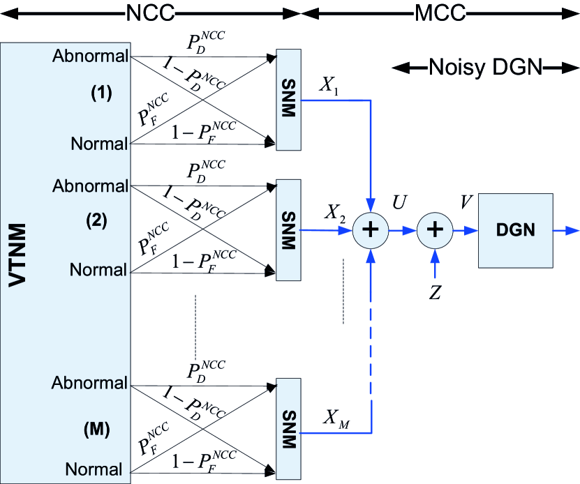
In this Subsection, the NADS performance is quantified using Theorem 1 on the NCC performance and considering the communication of SNMs over the MCC as discussed in Section III. Fig. 1 shows the modeling of the communication channels between the VTNM, the SNMs and the DGN. The NADS is composed of a broadcast channel with a common message followed by a Gaussian multiple access channel and an OR fusion rule.

Considering Fig. 1 and the communication of SNMs over the MCC, we have

U=j=1MXj.𝑈superscriptsubscript𝑗1𝑀subscript𝑋𝑗U=\sum\nolimits_{j=1}^{M}{{X_{j}}}. (35)

The event of abnormality detection alarm at the SNM j𝑗j, when the abnormality truly exists, is denoted by Djsubscript𝐷𝑗{D_{j}} and its complementary event is denoted by Djsubscriptsuperscript𝐷𝑗{D^{\prime}_{j}}. In this case, we consider QD=P(UG|𝑁𝑅𝑁𝐻)subscript𝑄𝐷𝑃𝑈conditional𝐺𝑁𝑅𝑁𝐻{Q_{D}}=P\left({\left.{U\geq G}\right|{\mathit{NR}}\neq{\mathit{NH}}}\right). Considering the spatially correlated observations of SNMs and using the OR-fusion rule, QDsubscript𝑄𝐷{Q_{D}} can be writen as follows

QD=1Pr{j=1MDj}.subscript𝑄𝐷1Prsuperscriptsubscript𝑗1𝑀subscriptsuperscript𝐷𝑗{Q_{D}}=1-\Pr\left\{{\bigcap\nolimits_{j=1}^{M}{{{D^{\prime}}_{j}}}}\right\}. (36)

The SNM j𝑗j alarms an abnormality over the NCC depending on its decision variable 𝑁𝑅j^^subscript𝑁𝑅𝑗\widehat{\mathit{NR_{j}}} in (26). Hence, to quantify the probability in (36), we need to derive the PDF of 𝐍𝐑^M=[𝑁𝑅^1𝑁𝑅^2𝑁𝑅^M]superscript^𝐍𝐑𝑀superscriptdelimited-[]subscript^𝑁𝑅1subscript^𝑁𝑅2subscript^𝑁𝑅𝑀missing-subexpressionmissing-subexpressionmissing-subexpressionmissing-subexpressionmissing-subexpressionmissing-subexpressionmissing-subexpressionmissing-subexpressionmissing-subexpressionmissing-subexpressionmissing-subexpressionmissing-subexpressionmissing-subexpressionmissing-subexpressionmissing-subexpressionmissing-subexpression{\widehat{{\bf{NR}}}^{M}}={[\begin{array}[]{*{20}{c}}{\widehat{\mathit{NR}}}_{1}&{\widehat{\mathit{NR}}}_{2}&\cdots&{\widehat{\mathit{NR}}}_{M}\end{array}]^{\dagger}}. The next lemma serves this purpose.

Refer to caption
Figure 1: Modeling of communication channels between VTNM, SNMs and the DGN.

Lemma 1. The decision variables of SNMs 𝐍𝐑^M=superscript^𝐍𝐑𝑀absent{\widehat{{\bf{NR}}}^{M}}= [𝑁𝑅^1𝑁𝑅^2𝑁𝑅^M]superscriptdelimited-[]subscript^𝑁𝑅1subscript^𝑁𝑅2subscript^𝑁𝑅𝑀missing-subexpressionmissing-subexpressionmissing-subexpressionmissing-subexpressionmissing-subexpressionmissing-subexpressionmissing-subexpressionmissing-subexpressionmissing-subexpressionmissing-subexpressionmissing-subexpressionmissing-subexpressionmissing-subexpressionmissing-subexpressionmissing-subexpressionmissing-subexpression{[\begin{array}[]{*{20}{c}}{\widehat{\mathit{NR}}}_{1}&{\widehat{\mathit{NR}}}_{2}&\cdots&{\widehat{\mathit{NR}}}_{M}\end{array}]^{\dagger}} are jointly Gaussian with mean 𝑁𝑅𝑁𝑅{\mathit{NR}} and (normalized) covariance matrix Ω𝑆𝐶superscriptΩ𝑆𝐶{\Omega^{\mathit{SC}}} in (11).

Proof. See Appendix B.

Using Lemma 1 and noting the decision region in (27), we have

QD=1𝑁𝐻τ𝑁𝐻+τ𝑁𝐻τ𝑁𝐻+τ1(2π)M/2σDM|Ω𝑆𝐶|1/2exp(12σD2(𝐍𝐑^M𝐍𝐑M)Ω𝑆𝐶1(𝐍𝐑^M𝐍𝐑M))d𝑁𝑅^1d𝑁𝑅^Msubscript𝑄𝐷1superscriptsubscript𝑁𝐻superscript𝜏𝑁𝐻superscript𝜏superscriptsubscript𝑁𝐻superscript𝜏𝑁𝐻superscript𝜏1superscript2𝜋𝑀/2superscriptsubscript𝜎𝐷𝑀superscriptsuperscriptΩ𝑆𝐶1/212superscriptsubscript𝜎𝐷2superscriptsuperscript^𝐍𝐑𝑀superscript𝐍𝐑𝑀superscriptsuperscriptΩ𝑆𝐶1superscript^𝐍𝐑𝑀superscript𝐍𝐑𝑀𝑑subscript^𝑁𝑅1𝑑subscript^𝑁𝑅𝑀\begin{array}[]{l}{Q_{D}}=1-\int\limits_{{\mathit{NH}}-\tau^{\prime}}^{{\mathit{NH}}+\tau^{\prime}}{...\int\limits_{{\mathit{NH}}-\tau^{\prime}}^{{\mathit{NH}}+\tau^{\prime}}}{}\\ \frac{1}{{{{\left({2\pi}\right)}^{{M\mathord{\left/{\vphantom{M2}}\right.\kern-1.2pt}2}}}\sigma_{D}^{M}{{\left|{{\Omega^{\mathit{SC}}}}\right|}^{{1\mathord{\left/{\vphantom{12}}\right.\kern-1.2pt}2}}}}}\exp\left({-\frac{1}{{2\sigma_{D}^{2}}}{{\left({{\widehat{{\bf{NR}}}^{M}}-{\bf{NR}}^{M}}\right)}^{\dagger}}{\Omega^{\mathit{SC}}}^{{}^{-1}}\left({{\widehat{{\bf{NR}}}^{M}}-{\bf{NR}}^{M}}\right)}\right)d\widehat{\mathit{{NR}}}_{1}\ldots d\widehat{\mathit{{NR}}}_{M}\end{array} (37)

where 𝐍𝐑M=[𝑁𝑅𝑁𝑅𝑁𝑅]1×Msuperscript𝐍𝐑𝑀subscriptdelimited-[]𝑁𝑅𝑁𝑅𝑁𝑅missing-subexpressionmissing-subexpressionmissing-subexpressionmissing-subexpressionmissing-subexpressionmissing-subexpressionmissing-subexpressionmissing-subexpressionmissing-subexpressionmissing-subexpressionmissing-subexpressionmissing-subexpressionmissing-subexpressionmissing-subexpressionmissing-subexpressionmissing-subexpression1𝑀{\bf{NR}}^{M}={\left[{\begin{array}[]{*{20}{c}}{{\mathit{NR}}}&{{\mathit{NR}}}&\cdots&{{\mathit{NR}}}\end{array}}\right]_{1\times M}} . In a similar manner, we consider Ejsubscript𝐸𝑗E_{j} as the false alarm event that SNM j𝑗j alarms an abnormality, when it does not exist in reality. The complementary event is denoted by Ejsubscriptsuperscript𝐸𝑗{E^{\prime}_{j}}. In this case, we consider QF=P(UG|𝑁𝑅=𝑁𝐻)subscript𝑄𝐹𝑃𝑈conditional𝐺𝑁𝑅𝑁𝐻{Q_{F}}=P\left({\left.{U\geq G}\right|{\mathit{NR}}={\mathit{NH}}}\right). Considering the spatially correlated observations of SNMs and using the OR-fusion rule, QFsubscript𝑄𝐹{Q_{F}} can be rewritten as follows

QF=1Pr{j=1MEj}subscript𝑄𝐹1Prsuperscriptsubscript𝑗1𝑀subscriptsuperscript𝐸𝑗{Q_{F}}=1-\Pr\left\{{\bigcap\nolimits_{j=1}^{M}{{{E^{\prime}}_{j}}}}\right\} (38)

Using Lemma 1 and noting the decision region in (27), we have

QF=1𝑁𝐻τ𝑁𝐻+τ𝑁𝐻τ𝑁𝐻+τ1(2π)M/2σDM|Ω𝑆𝐶|1/2exp(12σD2(𝐍𝐑^M𝐍𝐇M)Ω𝑆𝐶1(𝐍𝐑^M𝐍𝐇M))d𝑁𝑅^1d𝑁𝑅^Msubscript𝑄𝐹1superscriptsubscript𝑁𝐻superscript𝜏𝑁𝐻superscript𝜏superscriptsubscript𝑁𝐻superscript𝜏𝑁𝐻superscript𝜏1superscript2𝜋𝑀/2superscriptsubscript𝜎𝐷𝑀superscriptsuperscriptΩ𝑆𝐶1/212superscriptsubscript𝜎𝐷2superscriptsuperscript^𝐍𝐑𝑀superscript𝐍𝐇𝑀superscriptsuperscriptΩ𝑆𝐶1superscript^𝐍𝐑𝑀superscript𝐍𝐇𝑀𝑑subscript^𝑁𝑅1𝑑subscript^𝑁𝑅𝑀\begin{array}[]{l}{Q_{F}}=1-\int\limits_{{\mathit{NH}}-\tau^{\prime}}^{{\mathit{NH}}+\tau^{\prime}}{...\int\limits_{{\mathit{NH}}-\tau^{\prime}}^{{\mathit{NH}}+\tau^{\prime}}}{}\\ \frac{1}{{{{\left({2\pi}\right)}^{{M\mathord{\left/{\vphantom{M2}}\right.\kern-1.2pt}2}}}\sigma_{D}^{M}{{\left|{{\Omega^{\mathit{SC}}}}\right|}^{{1\mathord{\left/{\vphantom{12}}\right.\kern-1.2pt}2}}}}}\exp\left({-\frac{1}{{2\sigma_{D}^{2}}}{{\left({{\widehat{{\bf{NR}}}^{M}}-{\bf{NH}}^{M}}\right)}^{\dagger}}{\Omega^{\mathit{SC}}}^{{}^{-1}}\left({{\widehat{{\bf{NR}}}^{M}}-{\bf{NH}}^{M}}\right)}\right)d\widehat{\mathit{NR}}_{1}\ldots d\widehat{\mathit{NR}}_{M}\end{array} (39)

where 𝐍𝐇𝐌=[𝑁𝐻𝑁𝐻𝑁𝐻]1×Msuperscript𝐍𝐇𝐌subscriptdelimited-[]𝑁𝐻𝑁𝐻𝑁𝐻missing-subexpressionmissing-subexpressionmissing-subexpressionmissing-subexpressionmissing-subexpressionmissing-subexpressionmissing-subexpressionmissing-subexpressionmissing-subexpressionmissing-subexpressionmissing-subexpressionmissing-subexpressionmissing-subexpressionmissing-subexpressionmissing-subexpressionmissing-subexpression1𝑀{\bf{NH}^{M}}={\left[{\begin{array}[]{*{20}{c}}{\mathit{NH}}&{\mathit{NH}}&\cdots&{\mathit{NH}}\end{array}}\right]_{1\times M}} . If the observations of different SNMs are spatially independent, Ω𝑆𝐶superscriptΩ𝑆𝐶{\Omega^{\mathit{SC}}} is diagonal and (37) and (39) are simplified as follows [74],

QD=1(1PD𝑁𝐶𝐶)Msubscript𝑄𝐷1superscript1superscriptsubscript𝑃𝐷𝑁𝐶𝐶𝑀{Q_{D}}=1-{(1-P_{D}^{\mathit{NCC}})^{M}} (40)
QF=1(1PF𝑁𝐶𝐶)Msubscript𝑄𝐹1superscript1superscriptsubscript𝑃𝐹𝑁𝐶𝐶𝑀{Q_{F}}=1-{(1-P_{F}^{\mathit{NCC}})^{M}} (41)

where PF𝑁𝐶𝐶=η1superscriptsubscript𝑃𝐹𝑁𝐶𝐶subscript𝜂1P_{F}^{\mathit{NCC}}={\eta_{1}} and PM𝑁𝐶𝐶superscriptsubscript𝑃𝑀𝑁𝐶𝐶P_{M}^{\mathit{NCC}} is defined in (29).

At the DGN with the OR-rule, we are facing a channel with binary outputs. However, the input to the DGN is a noisy version of U𝑈U, i.e., V𝑉V, which is the basis for the decision on the possible presence of abnormality. The next theorem presents the corresponding decision region at the DGN based on maximum a-posteriori probability (MAP) rule. This is motivated to obtain a point estimate of the unobserved quantity of presence or non-presence of abnormality based on DGN observations.

Theorem 2. The decision region at the DGN based on MAP rule is given by

{H0:V<V𝑇𝐻𝑅H1:V>V𝑇𝐻𝑅cases:subscript𝐻0𝑉superscript𝑉𝑇𝐻𝑅:subscript𝐻1𝑉superscript𝑉𝑇𝐻𝑅\left\{\begin{array}[]{l}{H_{0}}:V<{V^{\mathit{THR}}}\\ {H_{1}}:V>{V^{\mathit{THR}}}\end{array}\right. (42)

where, V𝑇𝐻𝑅superscript𝑉𝑇𝐻𝑅V^{\mathit{THR}} is the minimum value of V𝑉V, satisfying the following inequality,

((1QF)P(H0)(1QD)P(H1))exp(V22σ𝑀𝐶𝐶2)+(QFP(H0)QDP(H1))1(1p0)l=1Mplexp((VlG)22σ𝑀𝐶𝐶2)>H0<0.limit-from1subscript𝑄𝐹𝑃subscript𝐻01subscript𝑄𝐷𝑃subscript𝐻1superscript𝑉22superscriptsubscript𝜎𝑀𝐶𝐶2subscript𝑄𝐹𝑃subscript𝐻0subscript𝑄𝐷𝑃subscript𝐻111subscript𝑝0superscriptsubscript𝑙1𝑀subscript𝑝𝑙superscript𝑉𝑙𝐺22superscriptsubscript𝜎𝑀𝐶𝐶2subscriptsuperscriptsubscript𝐻00\begin{array}[]{l}\left({\left({1-{Q_{F}}}\right)P({H_{0}})-\left({1-{Q_{D}}}\right)P({H_{1}})}\right)\exp\left({\frac{-{{V^{2}}}}{{2\sigma_{\mathit{MCC}}^{2}}}}\right)+\\ \left({{Q_{F}}P({H_{0}})-{Q_{D}}P({H_{1}})}\right)\frac{1}{{\left({1-{p_{0}}}\right)}}\sum\limits_{l=1}^{M}{{p_{l}}\exp\left({\frac{-{{{\left({V-lG}\right)}^{2}}}}{{2\sigma_{\mathit{MCC}}^{2}}}}\right)}\mathop{\mathop{>}\limits^{{H_{0}}}}\limits_{<}0.\end{array} (43)

In (43), pl=Pr{U=lG}subscript𝑝𝑙Pr𝑈𝑙𝐺{p_{l}}=\Pr\left\{{U=lG}\right\} for l{0,,M}𝑙0𝑀l\in\left\{{0,\ldots,M}\right\}, is given by

pl=P(H1)pl+P(H0)p′′lsubscript𝑝𝑙𝑃subscript𝐻1subscriptsuperscript𝑝𝑙𝑃subscript𝐻0subscriptsuperscript𝑝′′𝑙{p_{l}}=P\left({{H_{1}}}\right){{p^{\prime}}_{l}}+P\left({{H_{0}}}\right){{p^{\prime\prime}}_{l}} (44)

where plsubscriptsuperscript𝑝𝑙p^{\prime}_{l} and pl′′subscriptsuperscript𝑝′′𝑙p^{\prime\prime}_{l} are given by

pl=Pr{U=lG|H1}=(Ml)AAlACACMl1(2π)M/2σDM|Ω𝑆𝐶|1/2exp(12σD2(𝐍𝐑^M𝐍𝐑M)Ω𝑆𝐶1(𝐍𝐑^M𝐍𝐑M))d𝑁𝑅^1d𝑁𝑅^Msubscriptsuperscript𝑝𝑙Pr𝑈conditional𝑙𝐺subscript𝐻1𝑀missing-subexpressionmissing-subexpressionmissing-subexpressionmissing-subexpressionmissing-subexpressionmissing-subexpressionmissing-subexpressionmissing-subexpressionmissing-subexpressionmissing-subexpressionmissing-subexpressionmissing-subexpressionmissing-subexpressionmissing-subexpressionmissing-subexpressionmissing-subexpressionmissing-subexpressionmissing-subexpressionmissing-subexpression𝑙missing-subexpressionmissing-subexpressionmissing-subexpressionmissing-subexpressionmissing-subexpressionmissing-subexpressionmissing-subexpressionmissing-subexpressionmissing-subexpressionmissing-subexpressionmissing-subexpressionmissing-subexpressionmissing-subexpressionmissing-subexpressionmissing-subexpressionmissing-subexpressionmissing-subexpressionmissing-subexpressionmissing-subexpressionsubscriptsubscript𝐴subscript𝐴𝑙subscriptsubscriptsuperscript𝐴𝐶subscriptsuperscript𝐴𝐶𝑀𝑙1superscript2𝜋𝑀/2superscriptsubscript𝜎𝐷𝑀superscriptsuperscriptΩ𝑆𝐶1/212superscriptsubscript𝜎𝐷2superscriptsuperscript^𝐍𝐑𝑀superscript𝐍𝐑𝑀superscriptsuperscriptΩ𝑆𝐶1superscript^𝐍𝐑𝑀superscript𝐍𝐑𝑀𝑑subscript^𝑁𝑅1𝑑subscript^𝑁𝑅𝑀\begin{array}[]{l}{{p^{\prime}}_{l}}=\Pr\left\{{\left.{U=lG}\right|{H_{1}}}\right\}=\left({\begin{array}[]{*{20}{c}}M\\ l\end{array}}\right)\underbrace{\int_{A}{...}\int_{A}{}}_{l}\underbrace{\int_{{A^{C}}}{...}\int_{{A^{C}}}{}}_{M-l}\\ \frac{1}{{{{\left({2\pi}\right)}^{{M\mathord{\left/{\vphantom{M2}}\right.\kern-1.2pt}2}}}\sigma_{D}^{M}{{\left|{{\Omega^{\mathit{SC}}}}\right|}^{{1\mathord{\left/{\vphantom{12}}\right.\kern-1.2pt}2}}}}}\exp\left({-\frac{1}{{2\sigma_{D}^{2}}}{{\left({{\widehat{{\bf{NR}}}^{M}}-{\bf{NR}}^{M}}\right)}^{\dagger}}{\Omega^{\mathit{SC}}}^{{}^{-1}}\left({{\widehat{{\bf{NR}}}^{M}}-{\bf{NR}}^{M}}\right)}\right)d\widehat{\mathit{NR}}_{1}\ldots d\widehat{\mathit{NR}}_{M}\end{array} (45)
p′′l=Pr{U=lG|H0}=(Ml)AAlACACMl1(2π)M/2σDM|Ω𝑆𝐶|1/2exp(12σD2(𝐍𝐑^M𝐍𝐇M)Ω𝑆𝐶1(𝐍𝐑^M𝐍𝐇M))d𝑁𝑅^1d𝑁𝑅^M.subscriptsuperscript𝑝′′𝑙Pr𝑈conditional𝑙𝐺subscript𝐻0𝑀missing-subexpressionmissing-subexpressionmissing-subexpressionmissing-subexpressionmissing-subexpressionmissing-subexpressionmissing-subexpressionmissing-subexpressionmissing-subexpressionmissing-subexpressionmissing-subexpressionmissing-subexpressionmissing-subexpressionmissing-subexpressionmissing-subexpressionmissing-subexpressionmissing-subexpressionmissing-subexpressionmissing-subexpression𝑙missing-subexpressionmissing-subexpressionmissing-subexpressionmissing-subexpressionmissing-subexpressionmissing-subexpressionmissing-subexpressionmissing-subexpressionmissing-subexpressionmissing-subexpressionmissing-subexpressionmissing-subexpressionmissing-subexpressionmissing-subexpressionmissing-subexpressionmissing-subexpressionmissing-subexpressionmissing-subexpressionmissing-subexpressionsubscriptsubscript𝐴subscript𝐴𝑙subscriptsubscriptsuperscript𝐴𝐶subscriptsuperscript𝐴𝐶𝑀𝑙1superscript2𝜋𝑀/2superscriptsubscript𝜎𝐷𝑀superscriptsuperscriptΩ𝑆𝐶1/212superscriptsubscript𝜎𝐷2superscriptsuperscript^𝐍𝐑𝑀superscript𝐍𝐇𝑀superscriptsuperscriptΩ𝑆𝐶1superscript^𝐍𝐑𝑀superscript𝐍𝐇𝑀𝑑subscript^𝑁𝑅1𝑑subscript^𝑁𝑅𝑀\begin{array}[]{l}{{p^{\prime\prime}}_{l}}=\Pr\left\{{\left.{U=lG}\right|{H_{0}}}\right\}=\left({\begin{array}[]{*{20}{c}}M\\ l\end{array}}\right)\underbrace{\int_{A}{...}\int_{A}{}}_{l}\underbrace{\int_{{A^{C}}}{...}\int_{{A^{C}}}{}}_{M-l}\\ \frac{1}{{{{\left({2\pi}\right)}^{{M\mathord{\left/{\vphantom{M2}}\right.\kern-1.2pt}2}}}\sigma_{D}^{M}{{\left|{{\Omega^{\mathit{SC}}}}\right|}^{{1\mathord{\left/{\vphantom{12}}\right.\kern-1.2pt}2}}}}}\exp\left({-\frac{1}{{2\sigma_{D}^{2}}}{{\left({{\widehat{{\bf{NR}}}^{M}}-{\bf{NH}}^{M}}\right)}^{\dagger}}{\Omega^{\mathit{SC}}}^{{}^{-1}}\left({{\widehat{{\bf{NR}}}^{M}}-{\bf{NH}}^{M}}\right)}\right)d\widehat{\mathit{NR}}_{1}\ldots d\widehat{\mathit{NR}}_{M}.\end{array} (46)

A=𝑁𝐻τ+𝑁𝐻+τ\int_{A}\bullet=\int_{-\infty}^{{\mathit{NH}}-\tau^{\prime}}\bullet+\int_{{\mathit{NH}}+\tau^{\prime}}^{\infty}\bullet and AC=NHτNH+τ\int_{{A^{C}}}\bullet=\int_{NH-\tau^{\prime}}^{NH+\tau^{\prime}}\bullet,

Proof. See Appendix C.

Hence, the next theorem quantifies the NADS performance.

Theorem 3. The probabilities of detection and false alarm of NADS are given by

PD=𝒬(V𝑇𝐻𝑅σ𝑀𝐶𝐶)(1QD)+l=1M𝒬(V𝑇𝐻𝑅lGσ𝑀𝐶𝐶)pl1p0QDsubscript𝑃𝐷𝒬superscript𝑉𝑇𝐻𝑅subscript𝜎𝑀𝐶𝐶1subscript𝑄𝐷superscriptsubscript𝑙1𝑀𝒬superscript𝑉𝑇𝐻𝑅𝑙𝐺subscript𝜎𝑀𝐶𝐶subscriptsuperscript𝑝𝑙1subscriptsuperscript𝑝0subscript𝑄𝐷{P_{D}}={{\cal Q}}\left({\frac{{{V^{\mathit{THR}}}}}{{{\sigma_{\mathit{MCC}}}}}}\right)\left({1-{Q_{D}}}\right)+\frac{{\sum\nolimits_{l=1}^{M}{{{\cal Q}}\left({\frac{{{V^{\mathit{THR}}}-lG}}{{{\sigma_{\mathit{MCC}}}}}}\right){{p^{\prime}}_{l}}}}}{{1-{{p^{\prime}}_{0}}}}{Q_{D}} (47)
PF=𝒬(V𝑇𝐻𝑅σ𝑀𝐶𝐶)(1QF)+l=1M𝒬(V𝑇𝐻𝑅lGσ𝑀𝐶𝐶)p′′l1p′′0QFsubscript𝑃𝐹𝒬superscript𝑉𝑇𝐻𝑅subscript𝜎𝑀𝐶𝐶1subscript𝑄𝐹superscriptsubscript𝑙1𝑀𝒬superscript𝑉𝑇𝐻𝑅𝑙𝐺subscript𝜎𝑀𝐶𝐶subscriptsuperscript𝑝′′𝑙1subscriptsuperscript𝑝′′0subscript𝑄𝐹{P_{F}}={{\cal Q}}\left({\frac{{{V^{\mathit{THR}}}}}{{{\sigma_{\mathit{MCC}}}}}}\right)\left({1-{Q_{F}}}\right)+\frac{{\sum\nolimits_{l=1}^{M}{{{\cal Q}}\left({\frac{{{V^{\mathit{THR}}}-lG}}{{{\sigma_{\mathit{MCC}}}}}}\right){{p^{\prime\prime}}_{l}}}}}{{1-{{p^{\prime\prime}}_{0}}}}{Q_{F}} (48)

Proof. The proof is provided in Appendix D.

If the noise of SNMs are considered spatially independent, the next corollary presents the NADS probability of detection and false alarm.

Corollary 1. The probability of detection and false alarm of NADS for spatially independent NCCs are given by

PD=𝒬(V𝑇𝐻𝑅σ𝑀𝐶𝐶)(1PD𝑁𝐶𝐶)M+l=1MQ(V𝑇𝐻𝑅lGσ𝑀𝐶𝐶)pl1p0(1(1PD𝑁𝐶𝐶)M)subscript𝑃𝐷𝒬superscript𝑉𝑇𝐻𝑅subscript𝜎𝑀𝐶𝐶superscript1superscriptsubscript𝑃𝐷𝑁𝐶𝐶𝑀superscriptsubscript𝑙1𝑀𝑄superscript𝑉𝑇𝐻𝑅𝑙𝐺subscript𝜎𝑀𝐶𝐶subscriptsuperscript𝑝𝑙1subscriptsuperscript𝑝01superscript1superscriptsubscript𝑃𝐷𝑁𝐶𝐶𝑀{P_{D}}={{\cal Q}}\left({\frac{{{V^{\mathit{THR}}}}}{{{\sigma_{\mathit{MCC}}}}}}\right){(1-P_{D}^{\mathit{NCC}})^{M}}+\frac{{\sum\nolimits_{l=1}^{M}{Q\left({\frac{{{V^{\mathit{THR}}}-lG}}{{{\sigma_{\mathit{MCC}}}}}}\right){{p^{\prime}}_{l}}}}}{{1-{{p^{\prime}}_{0}}}}\left({1-{{(1-P_{D}^{\mathit{NCC}})}^{M}}}\right) (49)
PF=𝒬(V𝑇𝐻𝑅σ𝑀𝐶𝐶)(1PF𝑁𝐶𝐶)M+l=1MQ(V𝑇𝐻𝑅lGσ𝑀𝐶𝐶)p′′l1p′′0(1(1PF𝑁𝐶𝐶)M)subscript𝑃𝐹𝒬superscript𝑉𝑇𝐻𝑅subscript𝜎𝑀𝐶𝐶superscript1superscriptsubscript𝑃𝐹𝑁𝐶𝐶𝑀superscriptsubscript𝑙1𝑀𝑄superscript𝑉𝑇𝐻𝑅𝑙𝐺subscript𝜎𝑀𝐶𝐶subscriptsuperscript𝑝′′𝑙1subscriptsuperscript𝑝′′01superscript1superscriptsubscript𝑃𝐹𝑁𝐶𝐶𝑀{P_{F}}={{\cal Q}}\left({\frac{{{V^{\mathit{THR}}}}}{{{\sigma_{\mathit{MCC}}}}}}\right){(1-P_{F}^{\mathit{NCC}})^{M}}+\frac{{\sum\nolimits_{l=1}^{M}{Q\left({\frac{{{V^{\mathit{THR}}}-lG}}{{{\sigma_{\mathit{MCC}}}}}}\right){{p^{\prime\prime}}_{l}}}}}{{1-{{p^{\prime\prime}}_{0}}}}\left({1-{{(1-P_{F}^{\mathit{NCC}})}^{M}}}\right) (50)

where

pl=(Ml)(1PD𝑁𝐶𝐶)Ml(PD𝑁𝐶𝐶)lsubscriptsuperscript𝑝𝑙𝑀missing-subexpressionmissing-subexpressionmissing-subexpressionmissing-subexpressionmissing-subexpressionmissing-subexpressionmissing-subexpressionmissing-subexpressionmissing-subexpressionmissing-subexpressionmissing-subexpressionmissing-subexpressionmissing-subexpressionmissing-subexpressionmissing-subexpressionmissing-subexpressionmissing-subexpressionmissing-subexpressionmissing-subexpression𝑙missing-subexpressionmissing-subexpressionmissing-subexpressionmissing-subexpressionmissing-subexpressionmissing-subexpressionmissing-subexpressionmissing-subexpressionmissing-subexpressionmissing-subexpressionmissing-subexpressionmissing-subexpressionmissing-subexpressionmissing-subexpressionmissing-subexpressionmissing-subexpressionmissing-subexpressionmissing-subexpressionmissing-subexpressionsuperscript1superscriptsubscript𝑃𝐷𝑁𝐶𝐶𝑀𝑙superscriptsuperscriptsubscript𝑃𝐷𝑁𝐶𝐶𝑙{p^{\prime}_{l}}=\left({\begin{array}[]{*{20}{c}}M\\ l\end{array}}\right){\left({1-P_{D}^{\mathit{NCC}}}\right)^{M-l}}{\left({P_{D}^{\mathit{NCC}}}\right)^{l}} (51)
pl′′=(Ml)(1PF𝑁𝐶𝐶)Ml(PF𝑁𝐶𝐶)l.subscriptsuperscript𝑝′′𝑙𝑀missing-subexpressionmissing-subexpressionmissing-subexpressionmissing-subexpressionmissing-subexpressionmissing-subexpressionmissing-subexpressionmissing-subexpressionmissing-subexpressionmissing-subexpressionmissing-subexpressionmissing-subexpressionmissing-subexpressionmissing-subexpressionmissing-subexpressionmissing-subexpressionmissing-subexpressionmissing-subexpressionmissing-subexpression𝑙missing-subexpressionmissing-subexpressionmissing-subexpressionmissing-subexpressionmissing-subexpressionmissing-subexpressionmissing-subexpressionmissing-subexpressionmissing-subexpressionmissing-subexpressionmissing-subexpressionmissing-subexpressionmissing-subexpressionmissing-subexpressionmissing-subexpressionmissing-subexpressionmissing-subexpressionmissing-subexpressionmissing-subexpressionsuperscript1superscriptsubscript𝑃𝐹𝑁𝐶𝐶𝑀𝑙superscriptsuperscriptsubscript𝑃𝐹𝑁𝐶𝐶𝑙{p^{\prime\prime}_{l}}=\left({\begin{array}[]{*{20}{c}}M\\ l\end{array}}\right){\left({1-P_{F}^{\mathit{NCC}}}\right)^{M-l}}{\left({P_{F}^{\mathit{NCC}}}\right)^{l}}. (52)

Remark. 1. The analysis in Theorem 3 relies on an OR rule (1 out of M𝑀M rule). This can be extended to the case with m𝑚m out of M𝑀M rule at the DGN. Specifically, following similar steps, it is straight forward to show that the probabilities of detection and false alarm are given by

PD=l=0Mpl𝒬(V𝑇𝐻𝑅lGσMCC)subscript𝑃𝐷superscriptsubscript𝑙0𝑀subscriptsuperscript𝑝𝑙𝒬superscript𝑉𝑇𝐻𝑅𝑙𝐺subscript𝜎𝑀𝐶𝐶P_{D}=\sum_{l=0}^{M}p^{\prime}_{l}{\cal{Q}}\left(\frac{V^{\mathit{THR}}-lG}{\sigma_{MCC}}\right) (53)
PF=l=0Mpl′′𝒬(V𝑇𝐻𝑅lGσMCC).subscript𝑃𝐹superscriptsubscript𝑙0𝑀subscriptsuperscript𝑝′′𝑙𝒬superscript𝑉𝑇𝐻𝑅𝑙𝐺subscript𝜎𝑀𝐶𝐶P_{F}=\sum_{l=0}^{M}p^{\prime\prime}_{l}{\cal{Q}}\left(\frac{V^{\mathit{THR}}-lG}{\sigma_{MCC}}\right). (54)

where V𝑇𝐻𝑅superscript𝑉𝑇𝐻𝑅V^{\mathit{THR}} is smallest value of V𝑉V which satisfy the next inequality

((1QˇF)P(H0)(1QˇD)P(H1))2πσMCC2l=0m1pll=0m1plexp((VlG)22σMCC2)+limit-from1subscriptˇ𝑄𝐹𝑃subscript𝐻01subscriptˇ𝑄𝐷𝑃subscript𝐻12𝜋superscriptsubscript𝜎𝑀𝐶𝐶2superscriptsubscript𝑙0𝑚1subscript𝑝𝑙superscriptsubscript𝑙0𝑚1subscript𝑝𝑙superscript𝑉𝑙𝐺22superscriptsubscript𝜎𝑀𝐶𝐶2\displaystyle\frac{{\left({\left({1-{\check{Q}_{F}}}\right)P\left({{H_{0}}}\right)-\left({1-{\check{Q}_{D}}}\right)P\left({{H_{1}}}\right)}\right)}}{{\sqrt{2\pi\sigma_{MCC}^{2}}\sum\limits_{l=0}^{m-1}{{p_{l}}}}}\sum\limits_{l=0}^{m-1}{{p_{l}}}\exp\left({-\frac{{{{\left({V-lG}\right)}^{2}}}}{{2\sigma_{MCC}^{2}}}}\right)+
(QˇFP(H0)QˇDP(H1))2πσMCC2l=kMpll=mMplexp((VlG)22σMCC2)<>H00subscriptˇ𝑄𝐹𝑃subscript𝐻0subscriptˇ𝑄𝐷𝑃subscript𝐻12𝜋superscriptsubscript𝜎𝑀𝐶𝐶2superscriptsubscript𝑙𝑘𝑀subscript𝑝𝑙superscriptsubscript𝑙𝑚𝑀subscript𝑝𝑙superscript𝑉𝑙𝐺22superscriptsubscript𝜎𝑀𝐶𝐶2superscriptsuperscriptsubscript𝐻00\displaystyle\frac{{\left({{\check{Q}_{F}}P\left({{H_{0}}}\right)-{\check{Q}_{D}}P\left({{H_{1}}}\right)}\right)}}{{\sqrt{2\pi\sigma_{MCC}^{2}}\sum\limits_{l=k}^{M}{{p_{l}}}}}\sum\limits_{l=m}^{M}{{p_{l}}}\exp\left({-\frac{{{{\left({V-lG}\right)}^{2}}}}{{2\sigma_{MCC}^{2}}}}\right)\mathop{<}\limits^{\mathop{>}\limits^{{H_{0}}}}0 (55)

where QˇD=l=mMplsubscriptˇ𝑄𝐷superscriptsubscript𝑙𝑚𝑀subscriptsuperscript𝑝𝑙\check{Q}_{D}=\sum_{l=m}^{M}p^{\prime}_{l} and QˇF=l=mMpl′′subscriptˇ𝑄𝐹superscriptsubscript𝑙𝑚𝑀subscriptsuperscript𝑝′′𝑙\check{Q}_{F}=\sum_{l=m}^{M}p^{\prime\prime}_{l}. It is obvious that VTHRsuperscript𝑉THRV^{\rm THR} explicitly depends on m𝑚m. Indeed, for the case of m=1𝑚1m=1 replacing QDsubscript𝑄𝐷Q_{D} and QFsubscript𝑄𝐹Q_{F} in terms of plsubscriptsuperscript𝑝𝑙p^{\prime}_{l} and pl′′subscriptsuperscript𝑝′′𝑙p^{\prime\prime}_{l} in (45) and (46) leads to (53) and (54). Our experiments (not reported here) reveal that both PDsubscript𝑃𝐷P_{D} and PFsubscript𝑃𝐹P_{F} reduce as m𝑚m increases beyond one. Assuming SNMs have small PF𝑁𝐶𝐶superscriptsubscript𝑃𝐹𝑁𝐶𝐶P_{F}^{\mathit{NCC}} and PD𝑁𝐶𝐶superscriptsubscript𝑃𝐷𝑁𝐶𝐶P_{D}^{\mathit{NCC}} , and considering our application of early disease detection, in the sequel we focus on the 1 out M𝑀M rule and aim at improving the probability of detection, with a small and acceptable probability of false alarm. As elaborated, similar analysis can be carried out for the case of m𝑚m out of M𝑀M rule.

IV-B Computationally Efficient Performance Assessment

Performance evaluation of NADS based on the analyses in Theorem 2 and equations  (44), (45) and (46) is computationally challenging in general, due to the multiple nested integrals involved (especially for large number of SNMs). Therefore, in the next lemma we present approximations that enable more computationally efficient solutions.

Lemma 2. The probabilities plsubscriptsuperscript𝑝𝑙{p^{\prime}_{l}}, pl′′subscriptsuperscript𝑝′′𝑙{p^{\prime\prime}_{l}} and plsubscript𝑝𝑙{p_{l}} in (44), (45) and (46) are approximated by

pl(Ml)(1PDNCC)αMlM([𝟏]ΩSC1[𝟏])(PDNCC)αlM([𝟏]ΩSC1[𝟏]),subscriptsuperscript𝑝𝑙𝑀missing-subexpressionmissing-subexpressionmissing-subexpressionmissing-subexpressionmissing-subexpressionmissing-subexpressionmissing-subexpressionmissing-subexpressionmissing-subexpressionmissing-subexpressionmissing-subexpressionmissing-subexpressionmissing-subexpressionmissing-subexpressionmissing-subexpressionmissing-subexpressionmissing-subexpressionmissing-subexpressionmissing-subexpression𝑙missing-subexpressionmissing-subexpressionmissing-subexpressionmissing-subexpressionmissing-subexpressionmissing-subexpressionmissing-subexpressionmissing-subexpressionmissing-subexpressionmissing-subexpressionmissing-subexpressionmissing-subexpressionmissing-subexpressionmissing-subexpressionmissing-subexpressionmissing-subexpressionmissing-subexpressionmissing-subexpressionmissing-subexpressionsuperscript1superscriptsubscript𝑃𝐷𝑁𝐶𝐶𝛼𝑀𝑙𝑀superscriptdelimited-[]1superscriptΩ𝑆superscript𝐶1delimited-[]1superscriptsuperscriptsubscript𝑃𝐷𝑁𝐶𝐶𝛼𝑙𝑀superscriptdelimited-[]1superscriptΩ𝑆superscript𝐶1delimited-[]1{{p^{\prime}}_{l}}\approx\left({\begin{array}[]{*{20}{c}}M\\ l\end{array}}\right){\left({1-P_{D}^{NCC}}\right)^{\alpha\frac{{M-l}}{M}\left({{{\left[{\bf{1}}\right]}^{\dagger}}{\Omega^{S{C^{-1}}}}\left[{\bf{1}}\right]}\right)}}{\left({P_{D}^{NCC}}\right)^{\frac{{\alpha l}}{M}\left({{{\left[{\bf{1}}\right]}^{\dagger}}{\Omega^{S{C^{-1}}}}\left[{\bf{1}}\right]}\right)}}, (56)
p′′l(Ml)(1PFNCC)αMlM([𝟏]ΩSC1[𝟏])(PFNCC)αlM([𝟏]ΩSC1[𝟏]),subscriptsuperscript𝑝′′𝑙𝑀missing-subexpressionmissing-subexpressionmissing-subexpressionmissing-subexpressionmissing-subexpressionmissing-subexpressionmissing-subexpressionmissing-subexpressionmissing-subexpressionmissing-subexpressionmissing-subexpressionmissing-subexpressionmissing-subexpressionmissing-subexpressionmissing-subexpressionmissing-subexpressionmissing-subexpressionmissing-subexpressionmissing-subexpression𝑙missing-subexpressionmissing-subexpressionmissing-subexpressionmissing-subexpressionmissing-subexpressionmissing-subexpressionmissing-subexpressionmissing-subexpressionmissing-subexpressionmissing-subexpressionmissing-subexpressionmissing-subexpressionmissing-subexpressionmissing-subexpressionmissing-subexpressionmissing-subexpressionmissing-subexpressionmissing-subexpressionmissing-subexpressionsuperscript1superscriptsubscript𝑃𝐹𝑁𝐶𝐶𝛼𝑀𝑙𝑀superscriptdelimited-[]1superscriptΩ𝑆superscript𝐶1delimited-[]1superscriptsuperscriptsubscript𝑃𝐹𝑁𝐶𝐶𝛼𝑙𝑀superscriptdelimited-[]1superscriptΩ𝑆superscript𝐶1delimited-[]1{{p^{\prime\prime}}_{l}}\approx\left({\begin{array}[]{*{20}{c}}M\\ l\end{array}}\right){\left({1-P_{F}^{NCC}}\right)^{\alpha\frac{{M-l}}{M}\left({{{\left[{\bf{1}}\right]}^{\dagger}}{\Omega^{S{C^{-1}}}}\left[{\bf{1}}\right]}\right)}}{\left({P_{F}^{NCC}}\right)^{\frac{{\alpha l}}{M}\left({{{\left[{\bf{1}}\right]}^{\dagger}}{\Omega^{S{C^{-1}}}}\left[{\bf{1}}\right]}\right)}}, (57)
p~l=P(H1)p~l+P(H0)p~′′.subscript~𝑝𝑙𝑃subscript𝐻1subscriptsuperscript~𝑝𝑙𝑃subscript𝐻0superscript~𝑝′′{\tilde{p}_{l}}=P\left({{H_{1}}}\right){\tilde{p}^{\prime}_{l}}+P\left({{H_{0}}}\right)\tilde{p}^{\prime\prime}. (58)

where [𝟏]=[1,,1]M×1delimited-[]1subscriptsuperscript11𝑀1\left[{\bf{1}}\right]={\left[{1,...,1}\right]^{\dagger}_{M\times 1}} and α𝛼\alpha is a fitting parameter.

Proof. The proof is provided in Appendix E.

Since the DGN uses an OR-fusion rule, we have QD=1p0subscript𝑄𝐷1subscriptsuperscript𝑝0{Q_{D}}=1-{p^{\prime}_{0}} and QF=1p0′′subscript𝑄𝐹1subscriptsuperscript𝑝′′0{Q_{F}}=1-{p^{\prime\prime}_{0}}. Using (56) and (57) with l=0𝑙0l=0, we can approximate QDsubscript𝑄𝐷{Q_{D}} and QFsubscript𝑄𝐹Q_{F} in (37) and (39) for their efficient computation as follows:

Q~D=1(1PD𝑁𝐶𝐶)α[𝟏]Ω𝑆𝐶1[𝟏]subscript~𝑄𝐷1superscript1superscriptsubscript𝑃𝐷𝑁𝐶𝐶𝛼superscriptdelimited-[]1superscriptsuperscriptΩ𝑆𝐶1delimited-[]1{\tilde{Q}_{D}}=1-{(1-P_{D}^{\mathit{NCC}})^{\alpha{{\left[{\bf{1}}\right]}^{\dagger}}{\Omega^{\mathit{SC}}}^{{}^{-1}}\left[{\bf{1}}\right]}} (59)
Q~F=1(1PF𝑁𝐶𝐶)α[𝟏]Ω𝑆𝐶1[𝟏]subscript~𝑄𝐹1superscript1superscriptsubscript𝑃𝐹𝑁𝐶𝐶𝛼superscriptdelimited-[]1superscriptsuperscriptΩ𝑆𝐶1delimited-[]1{\tilde{Q}_{F}}=1-{(1-P_{F}^{\mathit{NCC}})^{\alpha{{\left[{\bf{1}}\right]}^{\dagger}}{\Omega^{\mathit{SC}}}^{{}^{-1}}\left[{\bf{1}}\right]}} (60)

Using the results of Lemma 2 and Corollary 1, computationally efficient expressions for PDsubscript𝑃𝐷P_{D} and PFsubscript𝑃𝐹P_{F} are obtained by replacing plsubscript𝑝𝑙p_{l}, plsubscriptsuperscript𝑝𝑙p^{\prime}_{l}, pl′′subscriptsuperscript𝑝′′𝑙p^{\prime\prime}_{l}, QDsubscript𝑄𝐷Q_{D} and QFsubscript𝑄𝐹Q_{F} with p~lsubscript~𝑝𝑙{\tilde{p}_{l}}, p~lsubscriptsuperscript~𝑝𝑙{\tilde{p}^{\prime}_{l}}, p~l′′subscriptsuperscript~𝑝′′𝑙{\tilde{p}^{\prime\prime}_{l}}, Q~Dsubscript~𝑄𝐷{\tilde{Q}_{D}} and Q~Fsubscript~𝑄𝐹{\tilde{Q}_{F}} , respectively.

V Numerical Results

In this Section, we present numerical results and assess the performance of the proposed NADS. In addition, the effects of different parameters including the temporal and spatial correlations of the SNM noise are studied. In the experiments of this Section, we assume that the observations of SNMs are temporally correlated by the correlation matrix in (20) and the spatial correlation matrix is Ω𝑆𝐶=[ωij𝑆𝐶]M×M,superscriptΩ𝑆𝐶subscriptdelimited-[]superscriptsubscript𝜔𝑖𝑗𝑆𝐶𝑀𝑀{\Omega^{\mathit{\mathit{SC}}}}={[\omega_{{}_{ij}}^{\mathit{\mathit{SC}}}]_{M\times M}}, and ωij𝑆𝐶=(1/4)|ij|\omega_{{}_{ij}}^{\mathit{\mathit{SC}}}=\left({{1\mathord{\left/{\vphantom{14}}\right.\kern-1.2pt}4}}\right){}^{\left|{i-j}\right|}. We also consider the volume of the sample size at 1000 nm3𝑛superscript𝑚3nm^{3}. Table IV presents the parameters of the numerical experiments.

Fig. 2 shows the probability of receiving no microscale messages at the DGN for spatially correlated noise of SNMs in presence of abnormality ( in  (45)) and its approximation (p0subscriptsuperscript𝑝0{p^{\prime}_{0}} in (56)) in terms of the number of SNMs, M𝑀M, for different values of observation time, n𝑛n. As evident the approximate expression p~0subscriptsuperscript~𝑝0{\tilde{p}^{\prime}_{0}} matches the analysis p0subscriptsuperscript𝑝0{p^{\prime}_{0}} reasonably well for the selected α=1.2𝛼1.2\alpha=1.2. As such in the subsequent numerical results, we set α=1.2𝛼1.2\alpha=1.2 when using the approximations.

Table V explains the presentation of numerical results in Figs 3(a)5(d). Two methods for obtaining the performance results are considered, which are labeled as approximate and numerical in the sequel. First, we elaborate the results and comment on how the two methods are compared. Fig. 3(a) shows the probability of miss-detection, PMsubscript𝑃𝑀{P_{M}} in terms of the number of SNMs in the sample size, M𝑀M for different values of observation time, n𝑛n and temporal correlation ρ𝜌\rho in spatially independent scenario. It is evident that even a small value of temporal correlation, e.g., ρ=0.1𝜌0.1\rho=0.1, greatly affects PMsubscript𝑃𝑀P_{M} . Fig. 3(b) shows PMsubscript𝑃𝑀P_{M} in terms of M𝑀M, for different values of observation time, n𝑛n in spatially correlated and temporally independent scenario. One sees that spatial correlation of SNM observations degrades PMsubscript𝑃𝑀{P_{M}}. For example, with M=8𝑀8M=8 and n=9𝑛9n=9, spatially independent SNM observations results in a 20 times smaller PMsubscript𝑃𝑀{P_{M}} when compared to the spatially correlated setting. Hence, if observations of SNMs are spatially correlated and we consider them as spatially independent, the reliability of NADS is substantially degraded. Figs 3(c) and  3(d) show PMsubscript𝑃𝑀{P_{M}} with σ𝑀𝐶𝐶=0.1subscript𝜎𝑀𝐶𝐶0.1{\sigma_{\mathit{MCC}}}=0.1 and σ𝑀𝐶𝐶=0.4subscript𝜎𝑀𝐶𝐶0.4{\sigma_{\mathit{MCC}}}=0.4 in terms of M𝑀M for different values of n𝑛n and ρ𝜌\rho in spatially and temporally correlated scenario. One sees that increasing σ𝑀𝐶𝐶subscript𝜎𝑀𝐶𝐶{\sigma_{\mathit{MCC}}} degrades PMsubscript𝑃𝑀P_{M}. Based on results in Figs 3(a)3(d), it is evident that the probability of miss-detection PMsubscript𝑃𝑀P_{M} obtained by the approximate method matches well with that computed based on the numerical method. Hence, the approximate method can be efficiently used to solve the design problem of (16).

Fig. 4(a) shows the probability of false alarm PFsubscript𝑃𝐹P_{F} in terms of M𝑀M, for different values of σ𝑀𝐶𝐶subscript𝜎𝑀𝐶𝐶{\sigma_{\mathit{MCC}}}. One sees that the behavior of PFsubscript𝑃𝐹{P_{F}} in terms of M𝑀M varies as σ𝑀𝐶𝐶subscript𝜎𝑀𝐶𝐶{\sigma_{\mathit{MCC}}} increases. For small values of σ𝑀𝐶𝐶subscript𝜎𝑀𝐶𝐶{\sigma_{\mathit{MCC}}}, the performance degradation is due to error in the NCC. As evident in (50), this performance result is valid for all values of n𝑛n and ρ𝜌\rho, since in this experiment, PF𝑁𝐶𝐶superscriptsubscript𝑃𝐹𝑁𝐶𝐶P_{F}^{\mathit{NCC}} is small (set to equality in (71)) and σ𝑀𝐶𝐶subscript𝜎𝑀𝐶𝐶\sigma_{\mathit{MCC}} is also small (effect of MCC is negligible on PFsubscript𝑃𝐹P_{F}). Moreover, one sees that any spatial or temporal correlation in SNM observations improves PFsubscript𝑃𝐹P_{F}. Fig. 4(b) shows PFsubscript𝑃𝐹P_{F} in terms of M𝑀M for different values of n𝑛n with σ𝑀𝐶𝐶=0.4subscript𝜎𝑀𝐶𝐶0.4\sigma_{\mathit{MCC}}=0.4. One sees that the point at which the behavior of the curves changes depends both on σ𝑀𝐶𝐶subscript𝜎𝑀𝐶𝐶{\sigma_{\mathit{MCC}}} and n𝑛n. From Figs 4(a) and  4(b), it is evident that the approximate method for computing PFsubscript𝑃𝐹P_{F} slightly overestimates the false alarm probability when compared to the numerical method (see Table V for all values of M𝑀M and n𝑛n. Hence, to avoid calculating multiple integrals in (37) and  (39), the proposed approximate method may be efficiently used to address the design problem in (16).

The presented results in recent figures may be used to solve the optimization problem of (16). For example, Figs 3(b) and 4(a) reveal that the optimized number of SNMs per unit size is M=7𝑀7M=7 for σ𝑀𝐶𝐶=0.1subscript𝜎𝑀𝐶𝐶0.1{\sigma_{\mathit{MCC}}}=0.1, when NCCs are spatially correlated and temporary independent for ξ=1106𝜉1superscript106\xi=1-{10^{-6}}, γ=105𝛾superscript105\gamma={10^{-5}}, σ𝑀𝐶𝐶=0.1subscript𝜎𝑀𝐶𝐶0.1\sigma_{\mathit{MCC}}=0.1 and n=9𝑛9n=9. Figs 3(d) and 4(b) indicate that in the same setting and temporary and spatially correlated NCCs with σ𝑀𝐶𝐶=0.4subscript𝜎𝑀𝐶𝐶0.4{\sigma_{\mathit{MCC}}}=0.4, we need to select M=23𝑀23M=23. Furthermore, Fig. 3(b) demonstrates a smaller PMsubscript𝑃𝑀{P_{M}} when SNM observations are spatially independent as opposed to when they are correlated. Hence, if we consider the correlated observations as independent observations in the analyses instead, we will underestimate the required number of SNMs, M𝑀M. For example, in the same setting with PF=105subscript𝑃𝐹superscript105P_{F}={10^{-5}} to achieve PM=106subscript𝑃𝑀superscript106{P_{M}}={10^{-6}} we find M=10𝑀10M=10 for spatially independent SNM observations. However, in the correlated scenario, we need at least M=13𝑀13M=13.

Figs 5(a) and  5(b) show PMsubscript𝑃𝑀P_{M} and PFsubscript𝑃𝐹P_{F} for NADS in terms of M𝑀M, for different values of PF𝑁𝐶𝐶superscriptsubscript𝑃𝐹𝑁𝐶𝐶P_{F}^{\mathit{NCC}} for spatially and temporary correlated NCCs. In Fig. 5(b), the results demonstrate that PFsubscript𝑃𝐹{P_{F}} increases with PF𝑁𝐶𝐶superscriptsubscript𝑃𝐹𝑁𝐶𝐶P_{F}^{\mathit{NCC}} and M𝑀M. The typical trade-off of false alarm and detection performance of SNM over the NCC is visible in Fig. 5(c). Interestingly, PF𝑁𝐶𝐶superscriptsubscript𝑃𝐹𝑁𝐶𝐶P_{F}^{\mathit{NCC}} affects the overall detection performance of NADS in the same way (Fig. 5(a)), as it directly influences the NCC detection performance PM𝑁𝐶𝐶superscriptsubscript𝑃𝑀𝑁𝐶𝐶P_{M}^{\mathit{NCC}}(Fig. 5(c)). These figures also demonstrate the effect of networking of the SNMs on the performance. Consider the performance of a single SNM in Fig. 5(c) at PF𝑁𝐶𝐶=106superscriptsubscript𝑃𝐹𝑁𝐶𝐶superscript106P_{F}^{\mathit{NCC}}={10^{-6}} and PM𝑁𝐶𝐶0.35superscriptsubscript𝑃𝑀𝑁𝐶𝐶0.35P_{M}^{\mathit{NCC}}\approx 0.35. According to results in  5(a) and  5(b), utilizing 20 SNMs leads to significantly improved PMsubscript𝑃𝑀P_{M} of 106superscript10610^{-6} and PF105subscript𝑃𝐹superscript105P_{F}\approx{10^{-5}} .

Our experiments (not reported here) reveal that the probability of miss-detection over the NCC noticeably reduces as parameter k𝑘k increases (this parameter may be used to indicate the disease progress level). Such a behavior then reflects in the overall system performance as depicted in Fig. 5(d). One sees that as k𝑘k increases, PMsubscript𝑃𝑀{P_{M}} reduces much faster with M𝑀M. The results indicate that if the competitor cell affects the molecular environment more strongly, the proposed NADS detects its presence more easily. A larger value of k𝑘k in (21), may be interpreted as a disease which has progressed further and hence has altered the status of the molecular environment more significantly from a healthy setting.

The setting of this paper in the special case of spatial and temporal independent noise of SNMs reduces to that of our earlier study in [21]. However, the presented analysis in this work is exact in the said setting, whereas the prior work relies on certain approximations. Specifically, our extensive numerical results show that the approximated analyses of PF and PM in [21] are respectively a good approximation and an upper bound for the exact values presented here.

TABLE IV: Parameters of numerical results for Figs 2-5(d), X:Y:Z denotes the range of parameter as [X,Z] with step size Y, G=1𝐺1G=1, 𝑁𝐻=1𝑁𝐻1\mathit{NH}=1 , vol=1000[nm3]𝑣𝑜𝑙1000delimited-[]𝑛superscript𝑚3vol=1000[nm^{3}].
Parameter σ𝑀𝐶𝐶subscript𝜎𝑀𝐶𝐶{\sigma_{\mathit{MCC}}} η1subscript𝜂1{\eta_{1}} n𝑛n k𝑘k
Figs 3(a)-3(c) 0.1 106superscript10610^{-6} 1:2:9 2
Figs 3(d) and 4(b) 0.4 106superscript10610^{-6} 1:2:9 2
Fig. 4(a) 0.1, 0.2:0.2:1 106superscript10610^{-6} 9 2
Figs 5(a)5(c) 0.1 [106105104103102101]delimited-[]superscript106superscript105superscript104superscript103superscript102superscript101[10^{-6}10^{-5}10^{-4}10^{-3}10^{-2}10^{-1}] 9 2
Fig. 5(d) 0.1 0.1 1 1.75:0.5:3.25
Refer to caption
Figure 2: The probability of receiving no microscale messages at DGN over the spatially and temporally correlated noise of SNMs in presence of abnormality (Solid lines: p0subscriptsuperscript𝑝0{p^{\prime}_{0}} in (45)) and approximation of p0subscriptsuperscript𝑝0{p^{\prime}_{0}} (Markers: p~0subscriptsuperscript~𝑝0{\tilde{p}^{\prime}_{0}} in (56)), in terms of M𝑀M for different values of n𝑛n with ρ=0.1𝜌0.1\rho=0.1.
TABLE V: Numerical results presentation specification for Figs 3-5
Method Type of Curve Spatially correlated QDsubscript𝑄𝐷Q_{D},QFsubscript𝑄𝐹Q_{F} plsubscriptsuperscript𝑝𝑙p^{\prime}_{l},pl′′subscriptsuperscript𝑝′′𝑙p^{\prime\prime}_{l} PMsubscript𝑃𝑀P_{M}, PFsubscript𝑃𝐹P_{F}
Numerical (Num.) Solid lines square-root\surd Numerically computed by (37) and  (39) Approximated by plsubscriptsuperscript𝑝𝑙p^{\prime}_{l} and pl′′subscriptsuperscript𝑝′′𝑙p^{\prime\prime}_{l} in (56) and  (57) (47) and (48)
Approximated (App.) Markers only square-root\surd Approximated by Q~Dsubscript~𝑄𝐷{\tilde{Q}_{D}} and Q~Fsubscript~𝑄𝐹{\tilde{Q}_{F}}  (59) and  (60) Approximated by plsubscriptsuperscript𝑝𝑙p^{\prime}_{l} and pl′′subscriptsuperscript𝑝′′𝑙p^{\prime\prime}_{l} in (56) and  (57) (47) and (48)
Exact formula spatially independent scenario (Sp. Ind.) Dashed-dotted lines ×\times  (40) and  (41)  (51) and  (52) (49) and (50)
(a)
Refer to caption
(b)
Refer to caption
(c)
Refer to caption
(d)
Refer to caption
Figure 3: (a) PMsubscript𝑃𝑀P_{M} vs. M𝑀M for different values of n𝑛n and ρ𝜌\rho in spatially independent and temporally correlated scenario (dashed-dotted ρ=0𝜌0\rho=0, dotted lines ρ=0.1𝜌0.1\rho=0.1 , dashed lines ρ=0.2𝜌0.2\rho=0.2 ) and σ𝑀𝐶𝐶=0.1subscript𝜎𝑀𝐶𝐶0.1{\sigma_{\mathit{MCC}}}=0.1. (b) PMsubscript𝑃𝑀P_{M} vs. M𝑀M for different values of n𝑛n in spatially independent/correlated and temporally independent scenario, ρ=0𝜌0\rho=0 and σ𝑀𝐶𝐶=0.1subscript𝜎𝑀𝐶𝐶0.1\sigma_{\mathit{MCC}}=0.1. (c) PMsubscript𝑃𝑀P_{M} vs. M𝑀M for different values of n𝑛n and ρ𝜌\rho in spatially and temporally correlated scenario. (Dotted lines ρ=0.1𝜌0.1\rho=0.1, dashed lines ρ=0.2𝜌0.2\rho=0.2) and σ𝑀𝐶𝐶=0.1subscript𝜎𝑀𝐶𝐶0.1{\sigma_{\mathit{MCC}}}=0.1. (d) PMsubscript𝑃𝑀P_{M} in terms of M𝑀M for different values of n𝑛n in spatially and temporally correlated scenario, for ρ=0.2𝜌0.2\rho=0.2 and σ𝑀𝐶𝐶=0.4subscript𝜎𝑀𝐶𝐶0.4\sigma_{\mathit{MCC}}=0.4 .
(a)
Refer to caption
(b)
Refer to caption
Figure 4: (a) PFsubscript𝑃𝐹P_{F} in terms of M𝑀M for different values of σ𝑀𝐶𝐶subscript𝜎𝑀𝐶𝐶\sigma_{\mathit{MCC}}, in spatially correlated/independent and temporary correlated scenario with ρ=0.2𝜌0.2\rho=0.2. (b) PFsubscript𝑃𝐹P_{F} in terms of M𝑀M for different values of n𝑛n in spatially and temporally correlated scenario, for ρ=0.2𝜌0.2\rho=0.2 and σ𝑀𝐶𝐶=0.4subscript𝜎𝑀𝐶𝐶0.4{\sigma_{\mathit{MCC}}}=0.4.
(a)
Refer to caption
(b)
Refer to caption
(c)
Refer to caption
(d)
Refer to caption
Figure 5: (a) PMsubscript𝑃𝑀P_{M} in terms of M𝑀M for different values of PF𝑁𝐶𝐶superscriptsubscript𝑃𝐹𝑁𝐶𝐶P_{F}^{\mathit{NCC}}. (b) PFsubscript𝑃𝐹P_{F} in terms of M𝑀M for different values of PF𝑁𝐶𝐶superscriptsubscript𝑃𝐹𝑁𝐶𝐶P_{F}^{\mathit{NCC}} all for ρ=0.2𝜌0.2\rho=0.2 and σ𝑀𝐶𝐶=0.1subscript𝜎𝑀𝐶𝐶0.1{\sigma_{\mathit{MCC}}}=0.1. (c) PMNCCsuperscriptsubscript𝑃𝑀𝑁𝐶𝐶P_{M}^{NCC} in terms of n𝑛n for different values of PF𝑁𝐶𝐶superscriptsubscript𝑃𝐹𝑁𝐶𝐶P_{F}^{\mathit{NCC}}, ρ=0.2.𝜌0.2\rho=0.2. (d) PMsubscript𝑃𝑀P_{M} in terms of M𝑀M for different values of k𝑘k, ρ=0.2𝜌0.2\rho=0.2 and σ𝑀𝐶𝐶=0.1subscript𝜎𝑀𝐶𝐶0.1{\sigma_{\mathit{MCC}}}=0.1.

VI Conclusions

An abnormality detection scheme for detection of competitor cells in a bio-molecular nano-network was proposed. This is motivated for the early detection and classification of diseases and enabling their timely and effective treatment. The proposed NADS is a two-tier network. The sensor nano-machines at the first tier act as receivers of a nano-communications channel modeling the molecular environment. The SNMs then communicate over a noisy channel to a data gathering node, which operates based on an OR fusion rule. The average number of received molecules serves as a feature for detecting the abnormalities at the SNMs. The detection performance of each SNM in presence of Gaussian observation noise was analyzed using a generalized likelihood ratio test. Moreover, the effects of temporal and spatial correlations of the SNMs observations on the detection performance were studied. The reported experiments results reveal that otherwise ignoring possibly existing temporal or spatial correlations would lead to noticeably inaccurate performance results. Next, quantifying the overall NADS detection performance, a design problem was set up that quantifies the minimum required concentration of SNMs for a desired level of NADS reliability. The solution determines the optimized operation of detectors for each of the NADS tiers. This in turn facilitates optimized abnormality detection with smallest possible side effects due to the injection of nano-sensors. The results indicate how effective fusion of the noisy observations collected from a number of sensor nano-machines with limited capabilities could provide an acceptable detection performance.

At the current stage of research on detection of diseases at the nano-scale, there are still many interesting open research problems. Here, we state a few of them. In this paper, the detection feature is set based on a mathematical modeling and certain valid approximations. Developing more precise models or obtaining the exact detection feature based on experimental measurements in the target tissue is an interesting research avenue. The side effects of injected SNMs on the molecular environment play an important role in the accuracy of the model and the performance of NADS. Hence, studying those effects is another key aspect of research in this field. Designing practical SNMs for detection of cancer or other diseases and taking the experimental constraints of those SNMs into consideration within the proposed NADS framework poses a number of other interesting and important research problems. Medical imaging is one approach to detection over the MCC; other approaches includes ultrasonic or terahertz communications. Realistic modeling of MCC noise is an interesting issue for enhancing the NADS performance for abnormality detection in a biomolecular environment.

VII Appendices

VII-A Proof of Theorem 1

The GLRT [73] for hypothesis test of (17) is given by

max𝑁𝑅𝑁𝐻P(𝐲jn|𝑁𝑅)P(𝐲jn|𝑁𝐻)=P(𝐲jn|𝑁𝑅^j)P(𝐲jn|𝑁𝐻)=1(2π)n/2σ𝑁𝐶𝐶n|ΩT|1/2exp(12σ𝑁𝐶𝐶2(𝐲jn𝐍𝐑^n)ΩT1(𝐲jn𝐍𝐑^n))1(2π)n/2σ𝑁𝐶𝐶n|ΩT|1/2exp(12σ𝑁𝐶𝐶2(𝐲jn𝐍𝐇n)ΩT1(𝐲jn𝐍𝐇n))>τ,subscript𝑁𝑅𝑁𝐻𝑃conditionalsuperscriptsubscript𝐲𝑗𝑛𝑁𝑅𝑃conditionalsuperscriptsubscript𝐲𝑗𝑛𝑁𝐻𝑃conditionalsuperscriptsubscript𝐲𝑗𝑛subscript^𝑁𝑅𝑗𝑃conditionalsuperscriptsubscript𝐲𝑗𝑛𝑁𝐻absent1superscript2𝜋𝑛/2superscriptsubscript𝜎𝑁𝐶𝐶𝑛superscriptsuperscriptΩ𝑇1/212superscriptsubscript𝜎𝑁𝐶𝐶2superscriptsuperscriptsubscript𝐲𝑗𝑛superscript^𝐍𝐑𝑛superscriptΩsuperscript𝑇1superscriptsubscript𝐲𝑗𝑛superscript^𝐍𝐑𝑛1superscript2𝜋𝑛/2superscriptsubscript𝜎𝑁𝐶𝐶𝑛superscriptsuperscriptΩ𝑇1/212superscriptsubscript𝜎𝑁𝐶𝐶2superscriptsuperscriptsubscript𝐲𝑗𝑛superscript𝐍𝐇𝑛superscriptΩsuperscript𝑇1superscriptsubscript𝐲𝑗𝑛superscript𝐍𝐇𝑛𝜏\begin{array}[]{l}\frac{{\mathop{\max}\limits_{{\mathit{NR}}\neq{\mathit{NH}}}P\left({\left.{{{\bf{y}}_{j}^{n}}}\right|{\mathit{NR}}}\right)}}{{P\left({\left.{{{\bf{y}}_{j}^{n}}}\right|{\mathit{NH}}}\right)}}=\frac{{P\left({\left.{{{\bf{y}}_{j}^{n}}}\right|\widehat{\mathit{NR}}_{j}}\right)}}{{P\left({\left.{{{\bf{y}}_{j}^{n}}}\right|{\mathit{NH}}}\right)}}=\\ \frac{{\frac{1}{{{{\left({2\pi}\right)}^{{n\mathord{\left/{\vphantom{n2}}\right.\kern-1.2pt}2}}}\sigma_{\mathit{NCC}}^{n}{{\left|{{\Omega^{T}}}\right|}^{{1\mathord{\left/{\vphantom{12}}\right.\kern-1.2pt}2}}}}}\exp\left({-\frac{1}{{2\sigma_{\mathit{NCC}}^{2}}}{{\left({{{\bf{y}}_{j}^{n}}-{\widehat{{\bf{NR}}}^{n}}}\right)}^{\dagger}}{\Omega^{{T^{-1}}}}\left({{{\bf{y}}_{j}^{n}}-{\widehat{{\bf{NR}}}^{n}}}\right)}\right)}}{{\frac{1}{{{{\left({2\pi}\right)}^{{n\mathord{\left/{\vphantom{n2}}\right.\kern-1.2pt}2}}}\sigma_{\mathit{NCC}}^{n}{{\left|{{\Omega^{T}}}\right|}^{{1\mathord{\left/{\vphantom{12}}\right.\kern-1.2pt}2}}}}}\exp\left({-\frac{1}{{2\sigma_{\mathit{NCC}}^{2}}}{{\left({{{\bf{y}}_{j}^{n}}-{\bf{NH}}^{n}}\right)}^{\dagger}}{\Omega^{{T^{{}^{-1}}}}}\left({{{\bf{y}}_{j}^{n}}-{\bf{NH}}^{n}}\right)}\right)}}>\tau,\end{array} (61)

where 𝐍𝐑^n=[𝑁𝑅^j]1×nsuperscript^𝐍𝐑𝑛subscriptdelimited-[]subscript^𝑁𝑅𝑗1𝑛{\widehat{{\bf{NR}}}^{n}}={\left[{\widehat{\mathit{NR}}_{j}}\right]_{1\times n}}, 𝐍𝐇n=[𝑁𝐻]1×nsuperscript𝐍𝐇𝑛subscriptdelimited-[]𝑁𝐻1𝑛{\bf{NH}}^{n}={\left[{\mathit{NH}}\right]_{1\times n}} and 𝑁𝑅^jsubscript^𝑁𝑅𝑗{\widehat{\mathit{NR}}_{j}} is given by (26). Simplifying (61) we have

exp{12σNCC2[l=1ni=1n(ylj𝑁𝑅^j)(yij𝑁𝑅^j)ψilTCl=1ni=1n(yljNH)(yijNH)ψilTC]}>τ.12superscriptsubscript𝜎𝑁𝐶𝐶2delimited-[]superscriptsubscript𝑙1𝑛superscriptsubscript𝑖1𝑛subscript𝑦𝑙𝑗subscript^𝑁𝑅𝑗subscript𝑦𝑖𝑗subscript^𝑁𝑅𝑗superscriptsubscript𝜓𝑖𝑙𝑇𝐶superscriptsubscript𝑙1𝑛superscriptsubscript𝑖1𝑛subscript𝑦𝑙𝑗𝑁𝐻subscript𝑦𝑖𝑗𝑁𝐻superscriptsubscript𝜓𝑖𝑙𝑇𝐶𝜏\exp\left\{{\frac{{-1}}{{2\sigma_{NCC}^{2}}}\left[{\sum\limits_{l=1}^{n}{\sum\limits_{i=1}^{n}{\left({{y_{lj}}-\widehat{\mathit{{NR}}}_{j}}\right)}}\left({{y_{ij}}-\widehat{\mathit{{NR}}}_{j}}\right)\psi_{il}^{TC}-\sum\limits_{l=1}^{n}{\sum\limits_{i=1}^{n}{\left({{y_{lj}}-NH}\right)}}\left({{y_{ij}}-NH}\right)\psi_{il}^{TC}}\right]}\right\}>\tau. (62)

Computing the natural Logarithm of (62), we obtain

12σNCC2{l=1ni=1n(ylj𝑁𝑅^j)(yij𝑁𝑅^j)ψilTCl=1ni=1n((ylj𝑁𝑅^j)+(𝑁𝑅^j𝑁𝐻))((yij𝑁𝑅^j)+(𝑁𝑅^j𝑁𝐻))ψilTC}>logτ.\begin{array}[]{l}\frac{{-1}}{{2\sigma_{NCC}^{2}}}\left\{{\sum\limits_{l=1}^{n}{\sum\limits_{i=1}^{n}{\left({{y_{lj}}-\widehat{\mathit{NR}}_{j}}\right)}}\left({{y_{ij}}-\widehat{\mathit{NR}}_{j}}\right)\psi_{il}^{TC}-}\right.\\ \left.{\sum\limits_{l=1}^{n}{\sum\limits_{i=1}^{n}{\left({\left({{y_{lj}}-\widehat{\mathit{NR}}_{j}}\right)+\left({\widehat{\mathit{NR}}_{j}-{\mathit{NH}}}\right)}\right)}}\left({\left({{y_{ij}}-\widehat{\mathit{NR}}_{j}}\right)+\left({\widehat{\mathit{NR}}_{j}-\mathit{NH}}\right)}\right)\psi_{il}^{TC}}\right\}>\log\tau.\end{array} (63)

Following some manipulations, we have

12σ𝑁𝐶𝐶2{l=1ni=1n(ylj𝑁𝑅^j)(𝑁𝑅^j𝑁𝐻)ψil𝑇𝐶l=1ni=1n(yij𝑁𝑅^j)(𝑁𝑅^j𝑁𝐻)ψil𝑇𝐶l=1ni=1n(𝑁𝑅^j𝑁𝐻)2ψil𝑇𝐶}>logτ.\begin{array}[]{l}\frac{{-1}}{{2\sigma_{\mathit{NCC}}^{2}}}\left\{{-\sum\limits_{l=1}^{n}{\sum\limits_{i=1}^{n}{\left({{y_{lj}}-\widehat{\mathit{NR}}_{j}}\right)\left({\widehat{\mathit{NR}}_{j}-{\mathit{NH}}}\right)}}}\right.\psi_{il}^{\mathit{TC}}-\\ \left.{{\rm{}}\sum\limits_{l=1}^{n}{\sum\limits_{i=1}^{n}{\left({{y_{ij}}-\widehat{\mathit{NR}}_{j}}\right)\left({\widehat{\mathit{NR}}_{j}-{\mathit{NH}}}\right)\psi_{il}^{\mathit{TC}}}}-\sum\limits_{l=1}^{n}{\sum\limits_{i=1}^{n}{{{\left({\widehat{\mathit{NR}}_{j}-{\mathit{NH}}}\right)}^{2}}\psi_{il}^{\mathit{TC}}}}}\right\}>\log\tau.\end{array} (64)

Replacing 𝑁𝑅^jsubscript^𝑁𝑅𝑗\widehat{\mathit{NR}}_{j} from (26) in the first and second terms of RHS of (64), we have

12σ𝑁𝐶𝐶2[l=1ni=1n(𝑁𝑅^j𝑁𝐻)2ψil𝑇𝐶]>logτ(𝑁𝑅^j𝑁𝐻)2>2σ𝑁𝐶𝐶2logτl=1ni=1nψil𝑇𝐶.12superscriptsubscript𝜎𝑁𝐶𝐶2delimited-[]superscriptsubscript𝑙1𝑛superscriptsubscript𝑖1𝑛superscriptsubscript^𝑁𝑅𝑗𝑁𝐻2superscriptsubscript𝜓𝑖𝑙𝑇𝐶𝜏superscriptsubscript^𝑁𝑅𝑗𝑁𝐻22superscriptsubscript𝜎𝑁𝐶𝐶2𝜏superscriptsubscript𝑙1𝑛superscriptsubscript𝑖1𝑛superscriptsubscript𝜓𝑖𝑙𝑇𝐶\frac{{-1}}{{2\sigma_{\mathit{NCC}}^{2}}}\left[{-\sum\limits_{l=1}^{n}{\sum\limits_{i=1}^{n}{{{\left({\widehat{\mathit{NR}}_{j}-\mathit{NH}}\right)}^{2}}\psi_{il}^{\mathit{TC}}}}}\right]>\log\tau\Rightarrow{\left({\widehat{\mathit{NR}}_{j}-{\mathit{NH}}}\right)^{2}}>\frac{{2\sigma_{\mathit{NCC}}^{2}\log\tau}}{{\sum\limits_{l=1}^{n}{\sum\limits_{i=1}^{n}{\psi_{il}^{\mathit{TC}}}}}}. (65)

With more simplification, the decision region for hypothesis test of (17) is obtained as

{H0𝑁𝐻τ<𝑁𝑅^j<𝑁𝐻+τH1𝑁𝑅^j>𝑁𝐻+τ𝑁𝑅^j<𝑁𝐻τ,casessubscript𝐻0𝑁𝐻superscript𝜏subscript^𝑁𝑅𝑗𝑁𝐻superscript𝜏missing-subexpressionmissing-subexpressionmissing-subexpressionmissing-subexpressionmissing-subexpressionmissing-subexpressionmissing-subexpressionmissing-subexpressionmissing-subexpressionmissing-subexpressionmissing-subexpressionmissing-subexpressionmissing-subexpressionmissing-subexpressionmissing-subexpressionmissing-subexpressionmissing-subexpressionmissing-subexpressionsubscript𝐻1subscript^𝑁𝑅𝑗𝑁𝐻superscript𝜏missing-subexpressionmissing-subexpressionmissing-subexpressionmissing-subexpressionmissing-subexpressionmissing-subexpressionmissing-subexpressionmissing-subexpressionmissing-subexpressionmissing-subexpressionmissing-subexpressionmissing-subexpressionmissing-subexpressionmissing-subexpressionmissing-subexpressionmissing-subexpressionmissing-subexpressionmissing-subexpressionmissing-subexpressionsubscript^𝑁𝑅𝑗𝑁𝐻superscript𝜏missing-subexpressionmissing-subexpressionmissing-subexpressionmissing-subexpressionmissing-subexpressionmissing-subexpressionmissing-subexpressionmissing-subexpressionmissing-subexpressionmissing-subexpressionmissing-subexpressionmissing-subexpressionmissing-subexpressionmissing-subexpressionmissing-subexpressionmissing-subexpressionmissing-subexpressionmissing-subexpressionmissing-subexpressionmissing-subexpressionmissing-subexpressionmissing-subexpressionmissing-subexpressionmissing-subexpressionmissing-subexpressionmissing-subexpressionmissing-subexpressionmissing-subexpressionmissing-subexpressionmissing-subexpressionmissing-subexpressionmissing-subexpressionmissing-subexpressionmissing-subexpressionmissing-subexpressionmissing-subexpressionmissing-subexpression\left\{{\begin{array}[]{*{20}{c}}{{H_{0}}}&{{\mathit{NH}}-\tau^{\prime}<\widehat{\mathit{NR}}_{j}<{\mathit{NH}}+\tau^{\prime}}\\ {{H_{1}}}&{\begin{array}[]{*{20}{c}}{\widehat{\mathit{NR}}_{j}>{\mathit{NH}}+\tau^{\prime}}\\ {\widehat{\mathit{NR}}_{j}<{\mathit{NH}}-\tau^{\prime},}\end{array}}\end{array}}\right. (66)

where

τ=Δ2σ𝑁𝐶𝐶2log(τ)/l=1ni=1nψil𝑇𝐶.superscriptΔsuperscript𝜏2superscriptsubscript𝜎𝑁𝐶𝐶2𝜏/superscriptsubscript𝑙1𝑛superscriptsubscript𝑖1𝑛superscriptsubscript𝜓𝑖𝑙𝑇𝐶\tau^{\prime}\buildrel\Delta\over{=}\sqrt{{{2\sigma_{\mathit{NCC}}^{2}\log\left(\tau\right)}\mathord{\left/{\vphantom{{2\sigma_{\mathit{NCC}}^{2}\log\left(\tau\right)}{\sum\limits_{l=1}^{n}{\sum\limits_{i=1}^{n}{\psi_{il}^{\mathit{TC}}}}}}}\right.\kern-1.2pt}{\sum\limits_{l=1}^{n}{\sum\limits_{i=1}^{n}{\psi_{il}^{\mathit{TC}}}}}}}. (67)

For deriving the false-alarm probability of a decision rule, we need to calculate the PDF of 𝑁𝑅^jsubscript^𝑁𝑅𝑗\widehat{\mathit{NR}}_{j} given in (26). The random variables yijsubscript𝑦𝑖𝑗y_{ij} are jointly Gaussian, hence their weighted summation is also Gaussian. When H0subscript𝐻0{H_{0}} is true, the mean of decision variable at the SNM, 𝑁𝑅^jsubscript^𝑁𝑅𝑗\widehat{\mathit{NR}}_{j} is 𝑁𝐻𝑁𝐻\mathit{NH} and its variance is given by [75]

σD2=(l=1ni=1nψil𝑇𝐶)2{l=1nvar(λl)+2q<lncov(λq,λl)}.superscriptsubscript𝜎𝐷2superscriptsuperscriptsubscript𝑙1𝑛superscriptsubscript𝑖1𝑛superscriptsubscript𝜓𝑖𝑙𝑇𝐶2superscriptsubscript𝑙1𝑛varsubscript𝜆𝑙2superscriptsubscript𝑞𝑙𝑛covsubscript𝜆𝑞subscript𝜆𝑙\sigma_{D}^{2}={\left({\sum\limits_{l=1}^{n}{\sum\limits_{i=1}^{n}{\psi_{il}^{\mathit{TC}}}}}\right)^{-2}}\left\{{\sum\limits_{l=1}^{n}{{\mathop{\rm var}}({\lambda_{l}})+2}\sum\limits_{q<l}^{n}{{\mathop{\rm cov}}({\lambda_{q}},{\lambda_{l}})}}\right\}. (68)

in which λl=ylji=1nψil𝑇𝐶subscript𝜆𝑙subscript𝑦𝑙𝑗superscriptsubscript𝑖1𝑛superscriptsubscript𝜓𝑖𝑙𝑇𝐶{\lambda_{l}}={y_{lj}}\sum\limits_{i=1}^{n}{\psi_{il}^{\mathit{TC}}}, the subscript of j𝑗j in λlsubscript𝜆𝑙\lambda_{l} is dropped due to homogeneous assumption of NCCs for each SNM, var(λl)=(i=1nψil𝑇𝐶)2σ𝑁𝐶𝐶2varsubscript𝜆𝑙superscriptsuperscriptsubscript𝑖1𝑛superscriptsubscript𝜓𝑖𝑙𝑇𝐶2superscriptsubscript𝜎𝑁𝐶𝐶2{\mathop{\rm var}}({\lambda_{l}})={\left({\sum\limits_{i=1}^{n}{\psi_{il}^{\mathit{TC}}}}\right)^{2}}\sigma_{\mathit{NCC}}^{2}, and cov(λq,λl)=(i=1nψil𝑇𝐶)(i=1nψil𝑇𝐶)ωql𝑇𝐶covsubscript𝜆𝑞subscript𝜆𝑙superscriptsubscript𝑖1𝑛superscriptsubscript𝜓𝑖𝑙𝑇𝐶superscriptsubscript𝑖1𝑛superscriptsubscript𝜓𝑖𝑙𝑇𝐶superscriptsubscript𝜔𝑞𝑙𝑇𝐶{\mathop{\rm cov}}({\lambda_{q}},{\lambda_{l}})=\left({\sum\limits_{i=1}^{n}{\psi_{il}^{\mathit{TC}}}}\right)\left({\sum\limits_{i=1}^{n}{\psi_{il}^{\mathit{TC}}}}\right)\omega_{ql}^{\mathit{TC}} σ𝑁𝐶𝐶2superscriptsubscript𝜎𝑁𝐶𝐶2\sigma_{\mathit{NCC}}^{2}. We have

σD2=(l=1ni=1nψil𝑇𝐶)2{l=1n(i=1nψil𝑇𝐶)2(σ𝑁𝐶𝐶2+2l=1n1q=l+1nωql𝑇𝐶σ𝑁𝐶𝐶2)}.superscriptsubscript𝜎𝐷2superscriptsuperscriptsubscript𝑙1𝑛superscriptsubscript𝑖1𝑛superscriptsubscript𝜓𝑖𝑙𝑇𝐶2superscriptsubscript𝑙1𝑛superscriptsuperscriptsubscript𝑖1𝑛superscriptsubscript𝜓𝑖𝑙𝑇𝐶2superscriptsubscript𝜎𝑁𝐶𝐶22superscriptsubscript𝑙1𝑛1superscriptsubscript𝑞𝑙1𝑛superscriptsubscript𝜔𝑞𝑙𝑇𝐶superscriptsubscript𝜎𝑁𝐶𝐶2\sigma_{D}^{2}={\left({\sum\limits_{l=1}^{n}{\sum\limits_{i=1}^{n}{\psi_{il}^{\mathit{TC}}}}}\right)^{-2}}\left\{{\sum\limits_{l=1}^{n}{{{\left({\sum\limits_{i=1}^{n}{\psi_{il}^{\mathit{TC}}}}\right)}^{2}}\left({\sigma_{\mathit{NCC}}^{2}+2\sum\limits_{l=1}^{n-1}{\sum\limits_{q=l+1}^{n}{\omega_{ql}^{\mathit{TC}}\sigma_{\mathit{NCC}}^{2}}}}\right)}}\right\}. (69)

Therefore, the false alarm probability can be expressed by

PF𝑁𝐶𝐶=1Pr{𝑁𝐻τ<𝒩(𝑁𝐻,σD2)<𝑁𝐻+τ|H0},superscriptsubscript𝑃𝐹𝑁𝐶𝐶1Pr𝑁𝐻superscript𝜏𝒩𝑁𝐻superscriptsubscript𝜎𝐷2bra𝑁𝐻superscript𝜏subscript𝐻0P_{F}^{\mathit{NCC}}=1-\Pr\left\{{\left.{\mathit{NH}-\tau^{\prime}<{{\cal N}}\left({\mathit{NH},\sigma_{D}^{2}}\right)<\mathit{NH}+\tau^{\prime}}\right|{H_{0}}}\right\}, (70)

and as we desire to have PF𝑁𝐶𝐶η1superscriptsubscript𝑃𝐹𝑁𝐶𝐶subscript𝜂1P_{F}^{\mathit{NCC}}\leq{\eta_{1}}, we obtain

2ϕ(τ/σD)11η1,2italic-ϕsuperscript𝜏/subscript𝜎𝐷11subscript𝜂12\phi\left({{{\tau^{\prime}}\mathord{\left/{\vphantom{{\tau^{\prime}}{\sigma_{D}}}}\right.\kern-1.2pt}{\sigma_{D}}}}\right)-1\geq 1-{\eta_{1}}, (71)

that is satisfied with equality, when we have

τ=σDϕ1(1η12).superscript𝜏subscript𝜎𝐷superscriptitalic-ϕ11subscript𝜂12\tau^{\prime}=\sigma_{D}{\phi^{-1}}\left({1-\frac{{{\eta_{1}}}}{2}}\right). (72)

According to the region of H1subscript𝐻1{H_{1}} in (66), PD𝑁𝐶𝐶superscriptsubscript𝑃𝐷𝑁𝐶𝐶P_{D}^{\mathit{NCC}} can be written as

PD𝑁𝐶𝐶=Pr{𝑁𝑅^j<𝑁𝐻τ,𝑁𝑅^j>𝑁𝐻+τ|H1},superscriptsubscript𝑃𝐷𝑁𝐶𝐶Prsubscript^𝑁𝑅𝑗𝑁𝐻superscript𝜏subscript^𝑁𝑅𝑗𝑁𝐻conditionalsuperscript𝜏subscript𝐻1P_{D}^{\mathit{NCC}}=\Pr\left\{{\left.{\widehat{\mathit{NR}}_{j}<{\mathit{NH}}-\tau^{\prime},\widehat{\mathit{NR}}_{j}>\mathit{NH}+\tau^{\prime}}\right|{H_{1}}}\right\}, (73)

and due to the Gaussian distribution of 𝑁𝑅^jsubscript^𝑁𝑅𝑗\widehat{\mathit{NR}}_{j}, we have

PD𝑁𝐶𝐶=Pr{𝒩(𝑁𝑅,σD2)<𝑁𝐻τ,𝒩(𝑁𝑅,σD2)>𝑁𝐻+τ}=1𝒬(𝑁𝐻τ𝑁𝑅σD2)+𝒬(𝑁𝐻+τ𝑁𝑅σD2).superscriptsubscript𝑃𝐷𝑁𝐶𝐶Pr𝒩𝑁𝑅superscriptsubscript𝜎𝐷2𝑁𝐻superscript𝜏𝒩𝑁𝑅superscriptsubscript𝜎𝐷2𝑁𝐻superscript𝜏absent1𝒬𝑁𝐻superscript𝜏𝑁𝑅superscriptsubscript𝜎𝐷2𝒬𝑁𝐻superscript𝜏𝑁𝑅superscriptsubscript𝜎𝐷2\begin{array}[]{l}P_{D}^{\mathit{NCC}}=\Pr\left\{{{{\cal N}}\left({{\mathit{NR}},\sigma_{D}^{2}}\right)<{\mathit{NH}}-\tau^{\prime},{{\cal N}}\left({{\mathit{NR}},\sigma_{D}^{2}}\right)>{\mathit{NH}}+\tau^{\prime}}\right\}=\\ 1-{{\cal Q}}\left({\frac{{{\mathit{NH}}-\tau^{\prime}-{\mathit{NR}}}}{{\sigma_{D}^{2}}}}\right)+{{\cal Q}}\left({\frac{{{\mathit{NH}}+\tau^{\prime}-{\mathit{NR}}}}{{\sigma_{D}^{2}}}}\right).\end{array} (74)

The relation of PDsubscript𝑃𝐷{P_{D}} and 𝑁𝑅𝑁𝑅\mathit{NR} is evident in (74). When a competitor cell is present in the NCC environment, 𝑁𝑅𝑁𝑅\mathit{NR} deviates from the 𝑁𝐻𝑁𝐻\mathit{NH}. For a specific type of competitor cell, considering (21) in (74), PD𝑁𝐶𝐶superscriptsubscript𝑃𝐷𝑁𝐶𝐶P_{D}^{\mathit{NCC}} can be obtained as

PD𝑁𝐶𝐶=1𝒬((𝑁𝐻τ(1±kσ𝑁𝐶𝐶)𝑁𝐻)/σD)+𝒬((𝑁𝐻+τ(1±kσ𝑁𝐶𝐶)𝑁𝐻)/σD)=1𝒬((τkσ𝑁𝐶𝐶𝑁𝐻)/(σD))+𝒬((τkσ𝑁𝐶𝐶𝑁𝐻)/(σD)).superscriptsubscript𝑃𝐷𝑁𝐶𝐶1𝒬𝑁𝐻superscript𝜏plus-or-minus1𝑘subscript𝜎𝑁𝐶𝐶𝑁𝐻/subscript𝜎𝐷𝒬𝑁𝐻superscript𝜏plus-or-minus1𝑘subscript𝜎𝑁𝐶𝐶𝑁𝐻/subscript𝜎𝐷absent1𝒬minus-or-plussuperscript𝜏𝑘subscript𝜎𝑁𝐶𝐶𝑁𝐻/subscript𝜎𝐷𝒬minus-or-plussuperscript𝜏𝑘subscript𝜎𝑁𝐶𝐶𝑁𝐻/subscript𝜎𝐷\begin{array}[]{l}P_{D}^{\mathit{NCC}}=1-{{\cal Q}}\left({{{\left({{\mathit{NH}}-\tau^{\prime}-\left({1\pm k{\sigma_{\mathit{NCC}}}}\right){\mathit{NH}}}\right)}\mathord{\left/{\vphantom{{\left({{\mathit{NH}}-\tau^{\prime}-\left({1\pm k{\sigma_{\mathit{NCC}}}}\right){\mathit{NH}}}\right)}{{\sigma_{D}}}}}\right.\kern-1.2pt}{{\sigma_{D}}}}}\right)+{{\cal Q}}\left({{{\left({{\mathit{NH}}+\tau^{\prime}-\left({1\pm k{\sigma_{\mathit{NCC}}}}\right){\mathit{NH}}}\right)}\mathord{\left/{\vphantom{{\left({{\mathit{NH}}+\tau^{\prime}-\left({1\pm k{\sigma_{\mathit{NCC}}}}\right){\mathit{NH}}}\right)}{{\sigma_{D}}}}}\right.\kern-1.2pt}{{\sigma_{D}}}}}\right)\\ {\rm{}}=1-{{\cal Q}}\left({{{\left({-\tau^{\prime}\mp k{\sigma_{\mathit{NCC}}}{\mathit{NH}}}\right)}\mathord{\left/{\vphantom{{\left({-\tau^{\prime}\mp k{\sigma_{\mathit{NCC}}}{\mathit{NH}}}\right)}{\left({{\sigma_{D}}}\right)}}}\right.\kern-1.2pt}{\left({{\sigma_{D}}}\right)}}}\right)+{{\cal Q}}\left({{{\left({\tau^{\prime}\mp k{\sigma_{\mathit{NCC}}}{\mathit{NH}}}\right)}\mathord{\left/{\vphantom{{\left({\tau^{\prime}\mp k{\sigma_{\mathit{NCC}}}{\mathit{NH}}}\right)}{\left({{\sigma_{D}}}\right)}}}\right.\kern-1.2pt}{\left({{\sigma_{D}}}\right)}}}\right).\end{array} (75)

Replacing τsuperscript𝜏\tau^{\prime} from (72) in (75), the following result is obtained

PD𝑁𝐶𝐶=1𝒬((σDϕ1(1η12)kσ𝑁𝐶𝐶𝑁𝐻)/σD)+𝒬((σDϕ1(1η12)kσ𝑁𝐶𝐶𝑁𝐻)/σD).superscriptsubscript𝑃𝐷𝑁𝐶𝐶limit-from1𝒬minus-or-plussubscript𝜎𝐷superscriptitalic-ϕ11subscript𝜂12𝑘subscript𝜎𝑁𝐶𝐶𝑁𝐻/subscript𝜎𝐷𝒬minus-or-plussubscript𝜎𝐷superscriptitalic-ϕ11subscript𝜂12𝑘subscript𝜎𝑁𝐶𝐶𝑁𝐻/subscript𝜎𝐷\begin{array}[]{l}P_{D}^{\mathit{NCC}}=1-\\ {{\cal Q}}\left({{{\left({-{\sigma_{D}}{\phi^{-1}}\left({1-\frac{{{\eta_{1}}}}{2}}\right)\mp k{\sigma_{\mathit{NCC}}}{\mathit{NH}}}\right)}\mathord{\left/{\vphantom{{\left({-{\sigma_{D}}{\phi^{-1}}\left({1-\frac{{{\eta_{1}}}}{2}}\right)\mp k{\sigma_{\mathit{NCC}}}{\mathit{NH}}}\right)}{{\sigma_{D}}}}}\right.\kern-1.2pt}{{\sigma_{D}}}}}\right)+{{\cal Q}}\left({{{\left({{\sigma_{D}}{\phi^{-1}}\left({1-\frac{{{\eta_{1}}}}{2}}\right)\mp k{\sigma_{\mathit{NCC}}}{\mathit{NH}}}\right)}\mathord{\left/{\vphantom{{\left({{\sigma_{D}}{\phi^{-1}}\left({1-\frac{{{\eta_{1}}}}{2}}\right)\mp k{\sigma_{\mathit{NCC}}}{\mathit{NH}}}\right)}{{\sigma_{D}}}}}\right.\kern-1.2pt}{{\sigma_{D}}}}}\right).\end{array} (76)

VII-B Proof of Lemma 1

It is evident in (26) that 𝑁𝑅^jsubscript^𝑁𝑅𝑗\widehat{\mathit{NR}}_{j} is a weighted sum of yijsubscript𝑦𝑖𝑗y_{ij}’s, which are jointly Gaussian distributed and hence their summation is Gaussian with mean 𝑁𝑅𝑁𝑅\mathit{NR}. The correlation coefficient of 𝑁𝑅^jsubscript^𝑁𝑅𝑗\widehat{\mathit{NR}}_{j} and 𝑁𝑅^qsubscript^𝑁𝑅𝑞\widehat{\mathit{NR}}_{q} is given by

cor(𝑁𝑅^j,𝑁𝑅^q)=E[(𝑁𝑅^j𝑁𝑅)(𝑁𝑅^q𝑁𝑅)]E[(𝑁𝑅^j𝑁𝑅)2]E[(𝑁𝑅^q𝑁𝑅)2].corsubscript^𝑁𝑅𝑗subscript^𝑁𝑅𝑞𝐸delimited-[]subscript^𝑁𝑅𝑗𝑁𝑅subscript^𝑁𝑅𝑞𝑁𝑅𝐸delimited-[]superscriptsubscript^𝑁𝑅𝑗𝑁𝑅2𝐸delimited-[]superscriptsubscript^𝑁𝑅𝑞𝑁𝑅2{\rm{cor}}(\widehat{\mathit{NR}}_{j},\widehat{\mathit{NR}}_{q})=\frac{{E\left[{\left({\widehat{\mathit{NR}}_{j}-{\mathit{NR}}}\right)\left({\widehat{\mathit{NR}}_{q}-\mathit{NR}}\right)}\right]}}{{\sqrt{E\left[{{{\left({\widehat{\mathit{NR}}_{j}-{\mathit{NR}}}\right)}^{2}}}\right]E\left[{{{\left({\widehat{\mathit{NR}}_{q}-{\mathit{NR}}}\right)}^{2}}}\right]}}}. (77)

Using (26), we obtain

cor(𝑁𝑅^j,𝑁𝑅^q)=E[(l=1ni=1nyljψil𝑇𝐶/l=1ni=1nψil𝑇𝐶𝑁𝑅)(l=1ni=1nylqψil𝑇𝐶/l=1ni=1nψil𝑇𝐶𝑁𝑅)]E[(l=1ni=1nyljψil𝑇𝐶/l=1ni=1nψil𝑇𝐶𝑁𝑅)2]E[(l=1ni=1nylqψil𝑇𝐶/l=1ni=1nψil𝑇𝐶𝑁𝑅)2],corsubscript^𝑁𝑅𝑗subscript^𝑁𝑅𝑞absent𝐸delimited-[]superscriptsubscript𝑙1𝑛superscriptsubscript𝑖1𝑛subscript𝑦𝑙𝑗superscriptsubscript𝜓𝑖𝑙𝑇𝐶/superscriptsubscript𝑙1𝑛superscriptsubscript𝑖1𝑛superscriptsubscript𝜓𝑖𝑙𝑇𝐶𝑁𝑅superscriptsubscript𝑙1𝑛superscriptsubscript𝑖1𝑛subscript𝑦𝑙𝑞superscriptsubscript𝜓𝑖𝑙𝑇𝐶/superscriptsubscript𝑙1𝑛superscriptsubscript𝑖1𝑛superscriptsubscript𝜓𝑖𝑙𝑇𝐶𝑁𝑅𝐸delimited-[]superscriptsuperscriptsubscript𝑙1𝑛superscriptsubscript𝑖1𝑛subscript𝑦𝑙𝑗superscriptsubscript𝜓𝑖𝑙𝑇𝐶/superscriptsubscript𝑙1𝑛superscriptsubscript𝑖1𝑛superscriptsubscript𝜓𝑖𝑙𝑇𝐶𝑁𝑅2𝐸delimited-[]superscriptsuperscriptsubscript𝑙1𝑛superscriptsubscript𝑖1𝑛subscript𝑦𝑙𝑞superscriptsubscript𝜓𝑖𝑙𝑇𝐶/superscriptsubscript𝑙1𝑛superscriptsubscript𝑖1𝑛superscriptsubscript𝜓𝑖𝑙𝑇𝐶𝑁𝑅2\begin{array}[]{l}{\rm{cor}}(\widehat{\mathit{NR}}_{j},\widehat{\mathit{NR}}_{q})=\\ \frac{{E\left[{\left({{{\sum\limits_{l=1}^{n}{\sum\limits_{i=1}^{n}{{y_{lj}}\psi_{il}^{\mathit{TC}}}}}\mathord{\left/{\vphantom{{\sum\limits_{l=1}^{n}{\sum\limits_{i=1}^{n}{{y_{lj}}\psi_{il}^{\mathit{TC}}}}}{\sum\limits_{l=1}^{n}{\sum\limits_{i=1}^{n}{\psi_{il}^{\mathit{TC}}}}}}}\right.\kern-1.2pt}{\sum\limits_{l=1}^{n}{\sum\limits_{i=1}^{n}{\psi_{il}^{\mathit{TC}}}}}}-{\mathit{NR}}}\right)\left({{{\sum\limits_{l=1}^{n}{\sum\limits_{i=1}^{n}{{y_{lq}}\psi_{il}^{\mathit{TC}}}}}\mathord{\left/{\vphantom{{\sum\limits_{l=1}^{n}{\sum\limits_{i=1}^{n}{{y_{lq}}\psi_{il}^{\mathit{TC}}}}}{\sum\limits_{l=1}^{n}{\sum\limits_{i=1}^{n}{\psi_{il}^{\mathit{TC}}}}}}}\right.\kern-1.2pt}{\sum\limits_{l=1}^{n}{\sum\limits_{i=1}^{n}{\psi_{il}^{\mathit{TC}}}}}}-{\mathit{NR}}}\right)}\right]}}{{\sqrt{E\left[{{{\left({{{\sum\limits_{l=1}^{n}{\sum\limits_{i=1}^{n}{{y_{lj}}\psi_{il}^{\mathit{TC}}}}}\mathord{\left/{\vphantom{{\sum\limits_{l=1}^{n}{\sum\limits_{i=1}^{n}{{y_{lj}}\psi_{il}^{\mathit{TC}}}}}{\sum\limits_{l=1}^{n}{\sum\limits_{i=1}^{n}{\psi_{il}^{\mathit{TC}}}}}}}\right.\kern-1.2pt}{\sum\limits_{l=1}^{n}{\sum\limits_{i=1}^{n}{\psi_{il}^{\mathit{TC}}}}}}-{\mathit{NR}}}\right)}^{2}}}\right]E\left[{{{\left({{{\sum\limits_{l=1}^{n}{\sum\limits_{i=1}^{n}{{y_{lq}}\psi_{il}^{\mathit{TC}}}}}\mathord{\left/{\vphantom{{\sum\limits_{l=1}^{n}{\sum\limits_{i=1}^{n}{{y_{lq}}\psi_{il}^{\mathit{TC}}}}}{\sum\limits_{l=1}^{n}{\sum\limits_{i=1}^{n}{\psi_{il}^{\mathit{TC}}}}}}}\right.\kern-1.2pt}{\sum\limits_{l=1}^{n}{\sum\limits_{i=1}^{n}{\psi_{il}^{\mathit{TC}}}}}}-{\mathit{NR}}}\right)}^{2}}}\right]}}},\end{array} (78)

and following some mathematical manipulation, we have

cor(𝑁𝑅^j,𝑁𝑅^q)=E[(l=1ni=1n(ylj𝑁𝑅)ψil𝑇𝐶)(l=1ni=1n(ylq𝑁𝑅)ψil𝑇𝐶)]E[(l=1ni=1n(ylj𝑁𝑅)ψil𝑇𝐶)2]E[(l=1ni=1n(ylq𝑁𝑅)ψil𝑇𝐶)2].corsubscript^𝑁𝑅𝑗subscript^𝑁𝑅𝑞𝐸delimited-[]superscriptsubscript𝑙1𝑛superscriptsubscript𝑖1𝑛subscript𝑦𝑙𝑗𝑁𝑅superscriptsubscript𝜓𝑖𝑙𝑇𝐶superscriptsubscript𝑙1𝑛superscriptsubscript𝑖1𝑛subscript𝑦𝑙𝑞𝑁𝑅superscriptsubscript𝜓𝑖𝑙𝑇𝐶𝐸delimited-[]superscriptsuperscriptsubscript𝑙1𝑛superscriptsubscript𝑖1𝑛subscript𝑦𝑙𝑗𝑁𝑅superscriptsubscript𝜓𝑖𝑙𝑇𝐶2𝐸delimited-[]superscriptsuperscriptsubscript𝑙1𝑛superscriptsubscript𝑖1𝑛subscript𝑦𝑙𝑞𝑁𝑅superscriptsubscript𝜓𝑖𝑙𝑇𝐶2{\rm{cor}}(\widehat{\mathit{NR}}_{j},\widehat{\mathit{NR}}_{q})=\frac{{E\left[{\left({\sum\limits_{l=1}^{n}{\sum\limits_{i=1}^{n}{\left({{y_{lj}}-{\mathit{NR}}}\right)\psi_{il}^{\mathit{TC}}}}}\right)\left({\sum\limits_{l=1}^{n}{\sum\limits_{i=1}^{n}{\left({{y_{lq}}-{\mathit{NR}}}\right)\psi_{il}^{\mathit{TC}}}}}\right)}\right]}}{{\sqrt{E\left[{{{\left({\sum\limits_{l=1}^{n}{\sum\limits_{i=1}^{n}{\left({{y_{lj}}-{\mathit{NR}}}\right)\psi_{il}^{\mathit{TC}}}}}\right)}^{2}}}\right]E\left[{{{\left({\sum\limits_{l=1}^{n}{\sum\limits_{i=1}^{n}{\left({{y_{lq}}-{\mathit{NR}}}\right)\psi_{il}^{\mathit{TC}}}}}\right)}^{2}}}\right]}}}. (79)

Using the assumption of separability of spatial and temporal correlation as discussed in Section II and some mathematical manipulations, we have

cor(𝑁𝑅^j,𝑁𝑅^q)=ωjq𝑆𝐶(l=1n(σ𝑁𝐶𝐶2(i=1nψil𝑇𝐶i=1nψil𝑇𝐶)+2k=l+1nωkl𝑇𝐶σ𝑁𝐶𝐶2i=1nψil𝑇𝐶i=1nψil𝑇𝐶))l=1n{(i=1nψil𝑇𝐶)2σ𝑁𝐶𝐶2+2k=l+1n(i=1nψil𝑇𝐶i=1nψil𝑇𝐶)ωkl𝑇𝐶σ𝑁𝐶𝐶2}=ωjq𝑆𝐶.corsubscript^𝑁𝑅𝑗subscript^𝑁𝑅𝑞superscriptsubscript𝜔𝑗𝑞𝑆𝐶superscriptsubscript𝑙1𝑛superscriptsubscript𝜎𝑁𝐶𝐶2superscriptsubscript𝑖1𝑛superscriptsubscript𝜓𝑖𝑙𝑇𝐶superscriptsubscript𝑖1𝑛superscriptsubscript𝜓𝑖𝑙𝑇𝐶2superscriptsubscript𝑘𝑙1𝑛superscriptsubscript𝜔𝑘𝑙𝑇𝐶superscriptsubscript𝜎𝑁𝐶𝐶2superscriptsubscript𝑖1𝑛superscriptsubscript𝜓𝑖𝑙𝑇𝐶superscriptsubscript𝑖1𝑛superscriptsubscript𝜓𝑖𝑙𝑇𝐶superscriptsubscript𝑙1𝑛superscriptsuperscriptsubscript𝑖1𝑛superscriptsubscript𝜓𝑖𝑙𝑇𝐶2superscriptsubscript𝜎𝑁𝐶𝐶22superscriptsubscript𝑘𝑙1𝑛superscriptsubscript𝑖1𝑛superscriptsubscript𝜓𝑖𝑙𝑇𝐶superscriptsubscript𝑖1𝑛superscriptsubscript𝜓𝑖𝑙𝑇𝐶superscriptsubscript𝜔𝑘𝑙𝑇𝐶superscriptsubscript𝜎𝑁𝐶𝐶2superscriptsubscript𝜔𝑗𝑞𝑆𝐶{\rm{cor}}(\widehat{\mathit{NR}}_{j},\widehat{\mathit{NR}}_{q})=\frac{{\omega_{jq}^{\mathit{SC}}\left({\sum\limits_{l=1}^{n}{\left({\sigma_{\mathit{NCC}}^{2}\left({\sum\limits_{i=1}^{n}{\psi_{il}^{\mathit{TC}}\sum\limits_{i=1}^{n}{\psi_{il}^{\mathit{TC}}}}}\right)+2\sum\limits_{k=l+1}^{n}{\omega_{kl}^{\mathit{TC}}\sigma_{\mathit{NCC}}^{2}\sum\limits_{i=1}^{n}{\psi_{il}^{\mathit{TC}}\sum\limits_{i=1}^{n}{\psi_{il}^{\mathit{TC}}}}}}\right)}}\right)}}{{\sum\limits_{l=1}^{n}{\left\{{{{\left({\sum\limits_{i=1}^{n}{\psi_{il}^{\mathit{TC}}}}\right)}^{2}}\sigma_{\mathit{NCC}}^{2}}\right.}{\rm{+2}}\sum\limits_{k=l+1}^{n}{\left({\sum\limits_{i=1}^{n}{\psi_{il}^{\mathit{TC}}}\sum\limits_{i=1}^{n}{\psi_{il}^{\mathit{TC}}}}\right)\left.{\omega_{kl}^{\mathit{TC}}\sigma_{\mathit{NCC}}^{2}}\right\}{\rm{}}}}}=\omega_{jq}^{\mathit{SC}}. (80)

VII-C Proof of Theorem 2

The MAP rule is written as

maxi{0,1}P(Hi|V)=(a)𝑃(Hi|V,W0)P(W0|V)+𝑃(Hi|V,W1)P(W1|V)=(b)maxi{0,1}𝑃(Hi|W0)P(W0|V)+𝑃(Hi|W1)P(W1|V)=(c)maxi{0,1}𝑃(W0|Hi)P(Hi)P(W0)P(W0|V)+𝑃(W1|Hi)P(Hi)P(W1)P(W1|V)subscript𝑖01𝑃conditionalsubscript𝐻𝑖𝑉superscripta𝑃conditionalsubscript𝐻𝑖𝑉subscript𝑊0𝑃conditionalsubscript𝑊0𝑉𝑃conditionalsubscript𝐻𝑖𝑉subscript𝑊1𝑃conditionalsubscript𝑊1𝑉superscript𝑏subscript𝑖01𝑃conditionalsubscript𝐻𝑖subscript𝑊0𝑃conditionalsubscript𝑊0𝑉𝑃conditionalsubscript𝐻𝑖subscript𝑊1𝑃conditionalsubscript𝑊1𝑉superscript𝑐subscript𝑖01𝑃conditionalsubscript𝑊0subscript𝐻𝑖𝑃subscript𝐻𝑖𝑃subscript𝑊0𝑃conditionalsubscript𝑊0𝑉𝑃conditionalsubscript𝑊1subscript𝐻𝑖𝑃subscript𝐻𝑖𝑃subscript𝑊1𝑃conditionalsubscript𝑊1𝑉\begin{array}[]{l}\mathop{\max}\limits_{i\in\left\{{0,1}\right\}}P\left({\left.{{H_{i}}}\right|V}\right)\mathop{=}\limits^{({\rm{a}})}{\mathop{P}\nolimits}\left({\left.{{H_{i}}}\right|V,{W_{0}}}\right)P\left({\left.{{W_{0}}}\right|V}\right)+{\mathop{P}\nolimits}\left({\left.{{H_{i}}}\right|V,{W_{1}}}\right)P\left({\left.{{W_{1}}}\right|V}\right)\\ \mathop{=}\limits^{(b)}\mathop{\max}\limits_{i\in\left\{{0,1}\right\}}{\mathop{P}\nolimits}\left({\left.{{H_{i}}}\right|{W_{0}}}\right)P\left({\left.{{W_{0}}}\right|V}\right)+{\mathop{P}\nolimits}\left({\left.{{H_{i}}}\right|{W_{1}}}\right)P\left({\left.{{W_{1}}}\right|V}\right)\\ \mathop{=}\limits^{(c)}\mathop{\max}\limits_{i\in\left\{{0,1}\right\}}\frac{{{\mathop{P}\nolimits}\left({\left.{{W_{0}}}\right|{H_{i}}}\right)P({H_{i}})}}{{P({W_{0}})}}P\left({\left.{{W_{0}}}\right|V}\right)+\frac{{{\mathop{P}\nolimits}\left({\left.{{W_{1}}}\right|{H_{i}}}\right)P({H_{i}})}}{{P({W_{1}})}}P\left({\left.{{W_{1}}}\right|V}\right)\end{array} (81)

where in the probability function of P()𝑃P\left(\bullet\right) event of V=v𝑉𝑣V=v is denoted by V𝑉V for brevity and events of W0subscript𝑊0{W_{0}}/W1subscript𝑊1{W_{1}} are defined as

{W0:j=1MXj<GW1:j=1MXjG.cases:subscript𝑊0superscriptsubscript𝑗1𝑀subscript𝑋𝑗𝐺missing-subexpressionmissing-subexpressionmissing-subexpressionmissing-subexpressionmissing-subexpressionmissing-subexpressionmissing-subexpressionmissing-subexpressionmissing-subexpressionmissing-subexpressionmissing-subexpressionmissing-subexpressionmissing-subexpressionmissing-subexpressionmissing-subexpressionmissing-subexpressionmissing-subexpressionmissing-subexpressionmissing-subexpression:subscript𝑊1superscriptsubscript𝑗1𝑀subscript𝑋𝑗𝐺missing-subexpressionmissing-subexpressionmissing-subexpressionmissing-subexpressionmissing-subexpressionmissing-subexpressionmissing-subexpressionmissing-subexpressionmissing-subexpressionmissing-subexpressionmissing-subexpressionmissing-subexpressionmissing-subexpressionmissing-subexpressionmissing-subexpressionmissing-subexpressionmissing-subexpressionmissing-subexpressionmissing-subexpression\left\{{\begin{array}[]{*{20}{c}}{{W_{0}}:\sum\nolimits_{j=1}^{M}{{X_{j}}}<G}\\ {{W_{1}}:\sum\nolimits_{j=1}^{M}{{X_{j}}}\geq G.}\end{array}}\right. (82)

In (81), (a) follows from the law of total probability, (b) from Markov property of HiWiVsubscript𝐻𝑖subscript𝑊𝑖𝑉{H_{i}}\to{W_{i}}\to V and (c) follows from the Bayes’ rule. Simplifying  (81), we have

P(W0|H0)P(H0)P(W0)P(W0|V)+P(W1|H0)P(H0)P(W1)P(W1|V)>H0<P(W0|H1)P(H1)P(W0)P(W0|V)+P(W1|H1)P(H1)P(W1)P(W1|V)(a)(1QF)P(H0)P(W0)P(W0|V)+QFP(H0)1P(W0)P(W1|V)>H0<(1QD)P(H1)P(W0)P(W0|V)+QDP(H1)1P(W0)P(W1|V)(b)(1QF)P(H0)P(W0)P(V|W0)P(W0)P(V)+QFP(H0)1P(W0)P(V|W1)P(W1)P(V)>H0<(1QD)P(H1)P(W0)P(V|W0)P(W0)P(V)+QDP(H1)1P(W0)P(V|W1)P(W1)P(V)(1QF)P(H0)P(V|W0)+QFP(H0)P(V|W1)>H0<(1QD)P(H1)P(V|W0)+QDP(H1)P(V|W1)Pconditionalsubscript𝑊0subscript𝐻0𝑃subscript𝐻0𝑃subscript𝑊0𝑃conditionalsubscript𝑊0𝑉Pconditionalsubscript𝑊1subscript𝐻0𝑃subscript𝐻0𝑃subscript𝑊1𝑃conditionalsubscript𝑊1𝑉subscriptsuperscriptsubscript𝐻0Pconditionalsubscript𝑊0subscript𝐻1𝑃subscript𝐻1𝑃subscript𝑊0𝑃conditionalsubscript𝑊0𝑉Pconditionalsubscript𝑊1subscript𝐻1𝑃subscript𝐻1𝑃subscript𝑊1𝑃conditionalsubscript𝑊1𝑉superscripta1subscript𝑄𝐹𝑃subscript𝐻0𝑃subscript𝑊0𝑃conditionalsubscript𝑊0𝑉subscript𝑄𝐹𝑃subscript𝐻01𝑃subscript𝑊0𝑃conditionalsubscript𝑊1𝑉subscriptsuperscriptsubscript𝐻01subscript𝑄𝐷𝑃subscript𝐻1𝑃subscript𝑊0𝑃conditionalsubscript𝑊0𝑉subscript𝑄𝐷𝑃subscript𝐻11𝑃subscript𝑊0𝑃conditionalsubscript𝑊1𝑉superscript𝑏1subscript𝑄𝐹𝑃subscript𝐻0𝑃subscript𝑊0𝑃conditional𝑉subscript𝑊0𝑃subscript𝑊0𝑃𝑉subscript𝑄𝐹𝑃subscript𝐻01𝑃subscript𝑊0𝑃conditional𝑉subscript𝑊1𝑃subscript𝑊1𝑃𝑉subscriptsuperscriptsubscript𝐻01subscript𝑄𝐷𝑃subscript𝐻1𝑃subscript𝑊0𝑃conditional𝑉subscript𝑊0𝑃subscript𝑊0𝑃𝑉subscript𝑄𝐷𝑃subscript𝐻11𝑃subscript𝑊0𝑃conditional𝑉subscript𝑊1𝑃subscript𝑊1𝑃𝑉absent1subscript𝑄𝐹𝑃subscript𝐻0𝑃conditional𝑉subscript𝑊0subscript𝑄𝐹𝑃subscript𝐻0𝑃conditional𝑉subscript𝑊1subscriptsuperscriptsubscript𝐻01subscript𝑄𝐷𝑃subscript𝐻1𝑃conditional𝑉subscript𝑊0subscript𝑄𝐷𝑃subscript𝐻1𝑃conditional𝑉subscript𝑊1\begin{array}[]{l}\frac{{{\mathop{\rm P}\nolimits}\left({\left.{{W_{0}}}\right|{H_{0}}}\right)P({H_{0}})}}{{P({W_{0}})}}P\left({\left.{{W_{0}}}\right|V}\right)+\frac{{{\mathop{\rm P}\nolimits}\left({\left.{{W_{1}}}\right|{H_{0}}}\right)P({H_{0}})}}{{P({W_{1}})}}P\left({\left.{{W_{1}}}\right|V}\right)\mathop{\mathop{>}\limits^{{H_{0}}}}\limits_{<}\\ \frac{{{\mathop{\rm P}\nolimits}\left({\left.{{W_{0}}}\right|{H_{1}}}\right)P({H_{1}})}}{{P({W_{0}})}}P\left({\left.{{W_{0}}}\right|V}\right)+\frac{{{\mathop{\rm P}\nolimits}\left({\left.{{W_{1}}}\right|{H_{1}}}\right)P({H_{1}})}}{{P({W_{1}})}}P\left({\left.{{W_{1}}}\right|V}\right)\mathop{\Rightarrow}\limits^{({\rm{a)}}}\\ \frac{{\left({1-{Q_{F}}}\right)P({H_{0}})}}{{P({W_{0}})}}P\left({\left.{{W_{0}}}\right|V}\right)+\frac{{{Q_{F}}P({H_{0}})}}{{1-P({W_{0}})}}P\left({\left.{{W_{1}}}\right|V}\right)\mathop{\mathop{>}\limits^{{H_{0}}}}\limits_{<}\frac{{\left({1-{Q_{D}}}\right)P({H_{1}})}}{{P({W_{0}})}}P\left({\left.{{W_{0}}}\right|V}\right)+\frac{{{Q_{D}}P({H_{1}})}}{{1-P({W_{0}})}}P\left({\left.{{W_{1}}}\right|V}\right)\mathop{\Rightarrow}\limits^{(b)}\\ \frac{{\left({1-{Q_{F}}}\right)P({H_{0}})}}{{P({W_{0}})}}\frac{{P\left({\left.V\right|{W_{0}}}\right)P\left({{W_{0}}}\right)}}{{P(V)}}+\frac{{{Q_{F}}P({H_{0}})}}{{1-P({W_{0}})}}\frac{{P\left({\left.V\right|{W_{1}}}\right)P\left({{W_{1}}}\right)}}{{P(V)}}\mathop{\mathop{>}\limits^{{H_{0}}}}\limits_{<}\\ \frac{{\left({1-{Q_{D}}}\right)P({H_{1}})}}{{P({W_{0}})}}\frac{{P\left({\left.V\right|{W_{0}}}\right)P\left({{W_{0}}}\right)}}{{P(V)}}+\frac{{{Q_{D}}P({H_{1}})}}{{1-P({W_{0}})}}\frac{{P\left({\left.V\right|{W_{1}}}\right)P\left({{W_{1}}}\right)}}{{P(V)}}\Rightarrow\\ \left({1-{Q_{F}}}\right)P({H_{0}})P\left({\left.V\right|{W_{0}}}\right)+{Q_{F}}P({H_{0}})P\left({\left.V\right|{W_{1}}}\right)\mathop{\mathop{>}\limits^{{H_{0}}}}\limits_{<}\left({1-{Q_{D}}}\right)P({H_{1}})P\left({\left.V\right|{W_{0}}}\right)+{Q_{D}}P({H_{1}})P\left({\left.V\right|{W_{1}}}\right)\end{array} (83)

where, (a) is derived based on definition of QFsubscript𝑄𝐹{Q_{F}} and QDsubscript𝑄𝐷{Q_{D}} respectively in (36) and (38), (b) is derived based on the Bayes’ rule. In (83), P(V|W0)𝑃conditional𝑉subscript𝑊0P\left({\left.V\right|{W_{0}}}\right) and P(V|W1)𝑃conditional𝑉subscript𝑊1P\left({\left.V\right|{W_{1}}}\right) are given by

P(V|W0)=12πσ𝑀𝐶𝐶2exp(V22σ𝑀𝐶𝐶2)𝑃conditional𝑉subscript𝑊012𝜋superscriptsubscript𝜎𝑀𝐶𝐶2superscript𝑉22superscriptsubscript𝜎𝑀𝐶𝐶2P\left({\left.V\right|{W_{0}}}\right)=\frac{1}{{\sqrt{2\pi\sigma_{\mathit{MCC}}^{2}}}}\exp\left({\frac{-{{{V}^{2}}}}{{2\sigma_{\mathit{MCC}}^{2}}}}\right) (84)
P(V|W1)=P(V|j=1MXjG)=P(V|j=1MXj=G.j=1MXj=MG)=(a)P(j=1MXj=G.j=1MXj=MG|V)P(V)P(j=1MXj=G.j=1MXj=MG)=(b)P(j=1MXj=G.j=1MXj=MG|V)P(V)1P(j=1MXj=0)=P({j=1MXj=G.j=1MXj=MG}V)1P(j=1MXj=0)=(c)P(({j=1MXj=G}V).({j=1MXj=MG}V))1P(j=1MXj=0)=(d)l=1MP({j=1MXj=lG}V)1P(j=1MXj=0)=j=1MP(V|j=1MXj=lG)P(j=1MXj=lG)1P(j=1MXj=0)=(e)1(1p0)2πσ𝑀𝐶𝐶2l=1Mplexp((VlG)22σ𝑀𝐶𝐶2).\begin{array}[]{l}P\left({\left.V\right|{W_{1}}}\right)=P\left({V\left|{\sum\limits_{j=1}^{M}{{X_{j}}}\geq G}\right.}\right)=P\left({V\left|{\sum\limits_{j=1}^{M}{{X_{j}}=G\cup}....\cup\sum\limits_{j=1}^{M}{{X_{j}}=MG}}\right.}\right)\\ \mathop{=}\limits^{({\rm{a}})}\frac{{P\left({\left.{\sum\limits_{j=1}^{M}{{X_{j}}=G\cup}....\cup\sum\limits_{j=1}^{M}{{X_{j}}=MG}}\right|V}\right)P\left(V\right)}}{{P\left({\sum\limits_{j=1}^{M}{{X_{j}}=G\cup}....\cup\sum\limits_{j=1}^{M}{{X_{j}}=MG}}\right)}}{\rm{}}\mathop{=}\limits^{(b)}\frac{{P\left({\left.{\sum\limits_{j=1}^{M}{{X_{j}}=G\cup}....\cup\sum\limits_{j=1}^{M}{{X_{j}}=MG}}\right|V}\right)P\left(V\right)}}{{1-P(\sum\limits_{j=1}^{M}{{X_{j}}}=0)}}\\ =\frac{{P\left({\left\{{\sum\limits_{j=1}^{M}{{X_{j}}=G\cup}....\cup\sum\limits_{j=1}^{M}{{X_{j}}=MG}}\right\}\cap V}\right)}}{{1-P(\sum\limits_{j=1}^{M}{{X_{j}}}=0)}}\mathop{{\rm{}}=}\limits^{(c)}\frac{{P\left({\left({\left\{{\sum\limits_{j=1}^{M}{{X_{j}}=G}}\right\}\cap V}\right)\cup....\cup\left({\left\{{\sum\limits_{j=1}^{M}{{X_{j}}=MG}}\right\}\cap V}\right)}\right)}}{{1-P(\sum\limits_{j=1}^{M}{{X_{j}}}=0)}}\\ \mathop{{\rm{}}=}\limits^{(d)}\frac{{\sum\nolimits_{l=1}^{M}{P\left({\left\{{\sum\limits_{j=1}^{M}{{X_{j}}=lG}}\right\}\cap V}\right)}}}{{1-P(\sum\limits_{j=1}^{M}{{X_{j}}}=0)}}{\rm{}}=\frac{{\sum\nolimits_{j=1}^{M}{P\left({V\left|{\sum\limits_{j=1}^{M}{{X_{j}}=lG}}\right.}\right)P(\sum\limits_{j=1}^{M}{{X_{j}}}=lG)}}}{{1-P(\sum\limits_{j=1}^{M}{{X_{j}}}=0)}}\\ \mathop{=}\limits^{(e)}\frac{1}{{\left({1-{p_{0}}}\right)\sqrt{2\pi\sigma_{\mathit{MCC}}^{2}}}}\sum\limits_{l=1}^{M}{{p_{l}}\exp\left({\frac{-{{{\left({V-lG}\right)}^{2}}}}{{2\sigma_{\mathit{MCC}}^{2}}}}\right)}.\end{array} (85)

Here, (a) follows from the Bayes’ rule, (b) follows from definition of event of Xjsubscript𝑋𝑗{X_{j}}, (c) follows from De Morgan’s law, (d) follows since the events Xj=lGsubscript𝑋𝑗𝑙𝐺X_{j}=lG, lfor-all𝑙\forall l are mutually exclusive, and (e) follows since the noise of MCC is Gaussian. Hence, replacing (84) and (85) in (83) we have

(1QF)P(H0)12πσ𝑀𝐶𝐶2exp(V22σ𝑀𝐶𝐶2)+QFP(H0)1(1p0)2πσ𝑀𝐶𝐶2l=1Mplexp((VlG)22σ𝑀𝐶𝐶2)>H0<(1QD)P(H1)12πσ𝑀𝐶𝐶2exp(V22σ𝑀𝐶𝐶2)+QDP(H1)1(1p0)2πσ𝑀𝐶𝐶2l=1Mplexp((VlG)22σ𝑀𝐶𝐶2),1subscript𝑄𝐹𝑃subscript𝐻012𝜋superscriptsubscript𝜎𝑀𝐶𝐶2superscript𝑉22superscriptsubscript𝜎𝑀𝐶𝐶2subscript𝑄𝐹𝑃subscript𝐻011subscript𝑝02𝜋superscriptsubscript𝜎𝑀𝐶𝐶2superscriptsubscript𝑙1𝑀subscript𝑝𝑙superscript𝑉𝑙𝐺22superscriptsubscript𝜎𝑀𝐶𝐶2subscriptsuperscriptsubscript𝐻01subscript𝑄𝐷𝑃subscript𝐻112𝜋superscriptsubscript𝜎𝑀𝐶𝐶2superscript𝑉22superscriptsubscript𝜎𝑀𝐶𝐶2subscript𝑄𝐷𝑃subscript𝐻111subscript𝑝02𝜋superscriptsubscript𝜎𝑀𝐶𝐶2superscriptsubscript𝑙1𝑀subscript𝑝𝑙superscript𝑉𝑙𝐺22superscriptsubscript𝜎𝑀𝐶𝐶2\begin{array}[]{l}\left({1-{Q_{F}}}\right)P({H_{0}})\frac{1}{{\sqrt{2\pi\sigma_{\mathit{MCC}}^{2}}}}\exp\left({\frac{-{{{{V}}^{2}}}}{{2\sigma_{\mathit{MCC}}^{2}}}}\right)+{Q_{F}}P({H_{0}})\frac{1}{{\left({1-{p_{0}}}\right)\sqrt{2\pi\sigma_{\mathit{MCC}}^{2}}}}\sum\limits_{l=1}^{M}{{p_{l}}\exp\left({\frac{-{{{\left({V-lG}\right)}^{2}}}}{{2\sigma_{\mathit{MCC}}^{2}}}}\right)}\mathop{\mathop{>}\limits^{{H_{0}}}}\limits_{<}\\ \left({1-{Q_{D}}}\right)P({H_{1}})\frac{1}{{\sqrt{2\pi\sigma_{\mathit{MCC}}^{2}}}}\exp\left({\frac{-{{{{V}}^{2}}}}{{2\sigma_{\mathit{MCC}}^{2}}}}\right)+{Q_{D}}P({H_{1}})\frac{1}{{\left({1-{p_{0}}}\right)\sqrt{2\pi\sigma_{\mathit{MCC}}^{2}}}}\sum\limits_{l=1}^{M}{{p_{l}}\exp\left({\frac{-{{{\left({V-lG}\right)}^{2}}}}{{2\sigma_{\mathit{MCC}}^{2}}}}\right)},\end{array} (86)

which simplifies to

((1QF)P(H0)(1QD)P(H1))exp(V22σ𝑀𝐶𝐶2)+(QFP(H0)QDP(H1))1(1p0)l=1Mplexp((VlG)22σ𝑀𝐶𝐶2)>H0<0.limit-from1subscript𝑄𝐹𝑃subscript𝐻01subscript𝑄𝐷𝑃subscript𝐻1superscript𝑉22superscriptsubscript𝜎𝑀𝐶𝐶2subscript𝑄𝐹𝑃subscript𝐻0subscript𝑄𝐷𝑃subscript𝐻111subscript𝑝0superscriptsubscript𝑙1𝑀subscript𝑝𝑙superscript𝑉𝑙𝐺22superscriptsubscript𝜎𝑀𝐶𝐶2subscriptsuperscriptsubscript𝐻00\begin{array}[]{l}\left({\left({1-{Q_{F}}}\right)P({H_{0}})-\left({1-{Q_{D}}}\right)P({H_{1}})}\right)\exp\left({\frac{-{{V^{2}}}}{{2\sigma_{\mathit{MCC}}^{2}}}}\right)+\\ \left({{Q_{F}}P({H_{0}})-{Q_{D}}P({H_{1}})}\right)\frac{1}{{\left({1-{p_{0}}}\right)}}\sum\limits_{l=1}^{M}{{p_{l}}\exp\left({\frac{-{{{\left({V-lG}\right)}^{2}}}}{{2\sigma_{\mathit{MCC}}^{2}}}}\right)}\mathop{\mathop{>}\limits^{{H_{0}}}}\limits_{<}0.\end{array} (87)

The decision region of DGN is then V<H0V𝑇𝐻𝑅𝑉superscriptsubscript𝐻0superscript𝑉𝑇𝐻𝑅V\mathop{<}\limits^{{H_{0}}}{V^{\mathit{THR}}}, where V𝑇𝐻𝑅superscript𝑉𝑇𝐻𝑅V^{\mathit{THR}} is derived numerically from (87).

VII-D Appendix D. Proof of Theorem 3

The probability of detection, PDsubscript𝑃𝐷{P_{D}}, is given by

PD=P(VH1|H1)=(a)P(VH1|H1,W0)P(W0|H1)+P(VH1|H1,W1)P(W1|H1)=(b)P(VH1|H1,W0)(1QD)+P(VH1|H1,W1)QD=(c)P(VH1|H1,j=1MXj=0)(1QD)+P(VH1|H1,j=1MXjG)QD=(d)P(VH1|H1,j=1MXj=0)(1QD)+l=1MP(VH1|j=1MXj=lG,H1)P(j=1MXj=lG|H1)1P(j=1MXj=0|H1)QD=𝒬(V𝑇𝐻𝑅σ𝑀𝐶𝐶)(1QD)+l=1M𝒬(V𝑇𝐻𝑅lGσ𝑀𝐶𝐶)pl1p0QD,subscript𝑃𝐷𝑃conditionalsubscript𝑉subscript𝐻1subscript𝐻1superscripta𝑃conditionalsubscript𝑉subscript𝐻1subscript𝐻1subscript𝑊0𝑃conditionalsubscript𝑊0subscript𝐻1𝑃conditionalsubscript𝑉subscript𝐻1subscript𝐻1subscript𝑊1𝑃conditionalsubscript𝑊1subscript𝐻1superscript𝑏𝑃conditionalsubscript𝑉subscript𝐻1subscript𝐻1subscript𝑊01subscript𝑄𝐷𝑃conditionalsubscript𝑉subscript𝐻1subscript𝐻1subscript𝑊1subscript𝑄𝐷superscript𝑐𝑃conditionalsubscript𝑉subscript𝐻1subscript𝐻1superscriptsubscript𝑗1𝑀subscript𝑋𝑗01subscript𝑄𝐷𝑃conditionalsubscript𝑉subscript𝐻1subscript𝐻1superscriptsubscript𝑗1𝑀subscript𝑋𝑗𝐺subscript𝑄𝐷superscript𝑑𝑃conditionalsubscript𝑉subscript𝐻1subscript𝐻1superscriptsubscript𝑗1𝑀subscript𝑋𝑗01subscript𝑄𝐷superscriptsubscript𝑙1𝑀𝑃conditionalsubscript𝑉subscript𝐻1superscriptsubscript𝑗1𝑀subscript𝑋𝑗𝑙𝐺subscript𝐻1𝑃superscriptsubscript𝑗1𝑀subscript𝑋𝑗conditional𝑙𝐺subscript𝐻11𝑃superscriptsubscript𝑗1𝑀subscript𝑋𝑗conditional0subscript𝐻1subscript𝑄𝐷absent𝒬superscript𝑉𝑇𝐻𝑅subscript𝜎𝑀𝐶𝐶1subscript𝑄𝐷superscriptsubscript𝑙1𝑀𝒬superscript𝑉𝑇𝐻𝑅𝑙𝐺subscript𝜎𝑀𝐶𝐶subscriptsuperscript𝑝𝑙1subscriptsuperscript𝑝0subscript𝑄𝐷\begin{array}[]{l}{P_{D}}=P\left({\left.{{V_{{H_{1}}}}}\right|{H_{1}}}\right)\mathop{=}\limits^{({\rm{a}})}P\left({\left.{{V_{{H_{1}}}}}\right|{H_{1}},{W_{0}}}\right)P\left({\left.{{W_{0}}}\right|{H_{1}}}\right)+P\left({\left.{{V_{{H_{1}}}}}\right|{H_{1}},{W_{1}}}\right)P\left({\left.{{W_{1}}}\right|{H_{1}}}\right)\\ \mathop{=}\limits^{(b)}P\left({\left.{{V_{{H_{1}}}}}\right|{H_{1}},{W_{0}}}\right)\left({1-{Q_{D}}}\right)+P\left({\left.{{V_{{H_{1}}}}}\right|{H_{1}},{W_{1}}}\right){Q_{D}}\\ \mathop{=}\limits^{(c)}P\left({\left.{{V_{{H_{1}}}}}\right|{H_{1}},\sum\nolimits_{j=1}^{M}{{X_{j}}=0}}\right)\left({1-{Q_{D}}}\right)+P\left({\left.{{V_{{H_{1}}}}}\right|{H_{1}},\sum\nolimits_{j=1}^{M}{{X_{j}}\geq G}}\right){Q_{D}}\\ \mathop{=}\limits^{(d)}P\left({\left.{{V_{{H_{1}}}}}\right|{H_{1}},\sum\nolimits_{j=1}^{M}{{X_{j}}=0}}\right)\left({1-{Q_{D}}}\right)+\frac{{\sum\nolimits_{l=1}^{M}{P\left({\left.{{V_{{H_{1}}}}}\right|\sum\limits_{j=1}^{M}{{X_{j}}=lG,{H_{1}}}}\right)P\left({\left.{\sum\limits_{j=1}^{M}{{X_{j}}}=lG}\right|{H_{1}}}\right)}}}{{1-P\left({\left.{\sum\limits_{j=1}^{M}{{X_{j}}=0}}\right|{H_{1}}}\right)}}{Q_{D}}\\ ={{\cal Q}}\left({\frac{{{V^{\mathit{THR}}}}}{{{\sigma_{\mathit{MCC}}}}}}\right)\left({1-{Q_{D}}}\right)+\frac{{\sum\nolimits_{l=1}^{M}{{{\cal Q}}\left({\frac{{{V^{\mathit{THR}}}-lG}}{{{\sigma_{\mathit{MCC}}}}}}\right){{p^{\prime}}_{l}}}}}{{1-{{p^{\prime}}_{0}}}}{Q_{D}},\end{array} (88)

where, VH1subscript𝑉𝐻1V_{H1} is the event of V>VTHR𝑉superscript𝑉THRV>V^{\rm{THR}}, (a) follows from the law of total probability, (b) is derived based on definitions of QFsubscript𝑄𝐹{Q_{F}} and QDsubscript𝑄𝐷{Q_{D}} respectively in (36) and (38), (c) is derived based on definitions of W0subscript𝑊0{W_{0}} and W1subscript𝑊1{W_{1}} in (82), and pl=Pr{U=lG|H1}subscriptsuperscript𝑝𝑙Pr𝑈conditional𝑙𝐺subscript𝐻1{p^{\prime}_{l}}=\Pr\left\{{\left.{U=lG}\right|{H_{1}}}\right\}, l[0,M]𝑙0𝑀l\in\left[{0,M}\right] is given by (45), and (d) is derived as follows,

P(VH1|H1,j=1MXjG)=P(VH1|H1(j=1MXj=G.j=1MXj=MG))=(a)P((j=1MXj=G.j=1MXj=MG)H1|VH1)P(VH1)P((j=1MXj=G.j=1MXj=MG)H1)=(b)P(({j=1MXj=G}VH1H1).({j=1MXj=MG}VH1H1))P((j=1MXj=G.j=1MXj=MG)H1)=(c)l=1MP({j=1MXj=lG}VH1H1)P((j=1MXj=G.j=1MXj=MG)H1)=(d)l=1MP(VH1|j=1MXj=lGH1)P(j=1MXj=lGH1)P((j=1MXj=G.j=1MXj=MG)H1)=(e)l=1MP(VH1|j=1MXj=lGH1)P(j=1MXj=lG|H1)P(H1)P((j=1MXj=G.j=1MXj=MG)|H1)P(H1)=(f)l=1MP(VH1|j=1MXj=lGH1)P(j=1MXj=lG|H1)1P(j=1MXj=0|H1).\begin{array}[]{l}P\left({{V_{{H_{1}}}}\left|{{H_{1}},\sum\limits_{j=1}^{M}{{X_{j}}}\geq G}\right.}\right)=P\left({{V_{{H_{1}}}}\left|{{H_{1}}\cap\left({\sum\limits_{j=1}^{M}{{X_{j}}=G\cup}....\cup\sum\limits_{j=1}^{M}{{X_{j}}=MG}}\right)}\right.}\right)\\ \mathop{\rm{=}}\limits^{\left({\rm{a}}\right)}\frac{{P\left({\left.{\left({\sum\limits_{j=1}^{M}{{X_{j}}=G\cup}....\cup\sum\limits_{j=1}^{M}{{X_{j}}=MG}}\right)\cap{H_{1}}}\right|{V_{{H_{1}}}}}\right)P\left({{V_{{H_{1}}}}}\right)}}{{P\left({\left({\sum\limits_{j=1}^{M}{{X_{j}}=G\cup}....\cup\sum\limits_{j=1}^{M}{{X_{j}}=MG}}\right)\cap{H_{1}}}\right)}}\mathop{{\rm{}}=}\limits^{\left(b\right)}\frac{{P\left({\left({\left\{{\sum\limits_{j=1}^{M}{{X_{j}}=G}}\right\}\cap{V_{{H_{1}}}}\cap{H_{1}}}\right)\cup....\cup\left({\left\{{\sum\limits_{j=1}^{M}{{X_{j}}=MG}}\right\}\cap{V_{{H_{1}}}}\cap{H_{1}}}\right)}\right)}}{{P\left({\left({\sum\limits_{j=1}^{M}{{X_{j}}=G\cup}....\cup\sum\limits_{j=1}^{M}{{X_{j}}=MG}}\right)\cap{H_{1}}}\right)}}\\ \mathop{=}\limits^{\left(c\right)}\frac{{\sum\nolimits_{l=1}^{M}{P\left({\left\{{\sum\limits_{j=1}^{M}{{X_{j}}=lG}}\right\}\cap{V_{{H_{1}}}}\cap{H_{1}}}\right)}}}{{P\left({\left({\sum\limits_{j=1}^{M}{{X_{j}}=G\cup}....\cup\sum\limits_{j=1}^{M}{{X_{j}}=MG}}\right)\cap{H_{1}}}\right)}}\mathop{=}\limits^{\left(d\right)}\frac{{\sum\nolimits_{l=1}^{M}{P\left({{V_{{H_{1}}}}\left|{\sum\limits_{j=1}^{M}{{X_{j}}=lG\cap{H_{1}}}}\right.}\right)P\left({\sum\limits_{j=1}^{M}{{X_{j}}}=lG\cap{H_{1}}}\right)}}}{{P\left({\left({\sum\limits_{j=1}^{M}{{X_{j}}=G\cup}....\cup\sum\limits_{j=1}^{M}{{X_{j}}=MG}}\right)\cap{H_{1}}}\right)}}\\ \mathop{=}\limits^{\left(e\right)}\frac{{\sum\nolimits_{l=1}^{M}{P\left({{V_{{H_{1}}}}\left|{\sum\limits_{j=1}^{M}{{X_{j}}=lG\cap{H_{1}}}}\right.}\right)P\left({\left.{\sum\limits_{j=1}^{M}{{X_{j}}}=lG}\right|{H_{1}}}\right)P\left({{H_{1}}}\right)}}}{{P\left({\left.{\left({\sum\limits_{j=1}^{M}{{X_{j}}=G\cup}....\cup\sum\limits_{j=1}^{M}{{X_{j}}=MG}}\right)}\right|{H_{1}}}\right)P\left({{H_{1}}}\right)}}\mathop{=}\limits^{\left(f\right)}\frac{{\sum\nolimits_{l=1}^{M}{P\left({{V_{{H_{1}}}}\left|{\sum\limits_{j=1}^{M}{{X_{j}}=lG\cap{H_{1}}}}\right.}\right)P\left({\left.{\sum\limits_{j=1}^{M}{{X_{j}}}=lG}\right|{H_{1}}}\right)}}}{{1-P\left({\left.{\sum\limits_{j=1}^{M}{{X_{j}}=0}}\right|{H_{1}}}\right)}}.\end{array} (89)

The steps in deriving (89) are similar to those in (85). In a similar way, the NADS probability of false alarm may be computed as

PF=P(VH0|H0)=P(VH0|H0,W0)P(W0|H0)+P(VH0|H0,W1)P(W1|H0)=P(VH0|H0,W0)(1QF)+P(VH0|H0,W1)QF=P(VH0|H0,j=1MXj=0)(1QF)+P(VH0|H0,j=1MXjG)QFP(VH0|H0,j=1MXj=0)(1QF)+l=1MP(VH0|j=1MXj=lG,H0)P(j=1MXj=lG|H0)1P(j=1MXj=0|H0)QF=𝒬(V𝑇𝐻𝑅σ𝑀𝐶𝐶)(1QF)+l=1M𝒬(V𝑇𝐻𝑅lGσ𝑀𝐶𝐶)p′′l1p′′0QF.subscript𝑃𝐹𝑃conditionalsubscript𝑉subscript𝐻0subscript𝐻0𝑃conditionalsubscript𝑉subscript𝐻0subscript𝐻0subscript𝑊0𝑃conditionalsubscript𝑊0subscript𝐻0𝑃conditionalsubscript𝑉subscript𝐻0subscript𝐻0subscript𝑊1𝑃conditionalsubscript𝑊1subscript𝐻0absent𝑃conditionalsubscript𝑉subscript𝐻0subscript𝐻0subscript𝑊01subscript𝑄𝐹𝑃conditionalsubscript𝑉subscript𝐻0subscript𝐻0subscript𝑊1subscript𝑄𝐹absent𝑃conditionalsubscript𝑉subscript𝐻0subscript𝐻0superscriptsubscript𝑗1𝑀subscript𝑋𝑗01subscript𝑄𝐹𝑃conditionalsubscript𝑉subscript𝐻0subscript𝐻0superscriptsubscript𝑗1𝑀subscript𝑋𝑗𝐺subscript𝑄𝐹𝑃conditionalsubscript𝑉subscript𝐻0subscript𝐻0superscriptsubscript𝑗1𝑀subscript𝑋𝑗01subscript𝑄𝐹superscriptsubscript𝑙1𝑀𝑃conditionalsubscript𝑉subscript𝐻0superscriptsubscript𝑗1𝑀subscript𝑋𝑗𝑙𝐺subscript𝐻0𝑃superscriptsubscript𝑗1𝑀subscript𝑋𝑗conditional𝑙𝐺subscript𝐻01𝑃superscriptsubscript𝑗1𝑀subscript𝑋𝑗conditional0subscript𝐻0subscript𝑄𝐹absent𝒬superscript𝑉𝑇𝐻𝑅subscript𝜎𝑀𝐶𝐶1subscript𝑄𝐹superscriptsubscript𝑙1𝑀𝒬superscript𝑉𝑇𝐻𝑅𝑙𝐺subscript𝜎𝑀𝐶𝐶subscriptsuperscript𝑝′′𝑙1subscriptsuperscript𝑝′′0subscript𝑄𝐹\begin{array}[]{l}{P_{F}}=P\left({\left.{{V_{{H_{0}}}}}\right|{H_{0}}}\right)=P\left({\left.{{V_{{H_{0}}}}}\right|{H_{0}},{W_{0}}}\right)P\left({\left.{{W_{0}}}\right|{H_{0}}}\right)+P\left({\left.{{V_{{H_{0}}}}}\right|{H_{0}},{W_{1}}}\right)P\left({\left.{{W_{1}}}\right|{H_{0}}}\right)\\ =P\left({\left.{{V_{{H_{0}}}}}\right|{H_{0}},{W_{0}}}\right)\left({1-{Q_{F}}}\right)+P\left({\left.{{V_{{H_{0}}}}}\right|{H_{0}},{W_{1}}}\right){Q_{F}}\\ =P\left({\left.{{V_{{H_{0}}}}}\right|{H_{0}},\sum\nolimits_{j=1}^{M}{{X_{j}}=0}}\right)\left({1-{Q_{F}}}\right)+P\left({\left.{{V_{{H_{0}}}}}\right|{H_{0}},\sum\nolimits_{j=1}^{M}{{X_{j}}\geq G}}\right){Q_{F}}\\ P\left({{V_{{H_{0}}}}\left|{{H_{0}},\sum\nolimits_{j=1}^{M}{{X_{j}}=0}}\right.}\right)\left({1-{Q_{F}}}\right)+\frac{{\sum\nolimits_{l=1}^{M}{P\left({{V_{{H_{0}}}}\left|{\sum\limits_{j=1}^{M}{{X_{j}}=lG,{H_{0}}}}\right.}\right)P\left({\left.{\sum\limits_{j=1}^{M}{{X_{j}}}=lG}\right|{H_{0}}}\right)}}}{{1-P\left({\left.{\sum\limits_{j=1}^{M}{{X_{j}}=0}}\right|{H_{0}}}\right)}}{Q_{F}}\\ ={{\cal Q}}\left({\frac{{{V^{\mathit{THR}}}}}{{{\sigma_{\mathit{MCC}}}}}}\right)\left({1-{Q_{F}}}\right)+\frac{{\sum\nolimits_{l=1}^{M}{{{\cal Q}}\left({\frac{{{V^{\mathit{THR}}}-lG}}{{{\sigma_{\mathit{MCC}}}}}}\right){{p^{\prime\prime}}_{l}}}}}{{1-{{p^{\prime\prime}}_{0}}}}{Q_{F}}.\end{array} (90)

where, VH0subscript𝑉𝐻0V_{H0} is the event of V<VTHR𝑉superscript𝑉THRV<V^{\rm{THR}}, pl′′=Pr{U=lG|H0}subscriptsuperscript𝑝′′𝑙Pr𝑈conditional𝑙𝐺subscript𝐻0{p^{\prime\prime}_{l}}=\Pr\left\{{\left.{U=lG}\right|{H_{0}}}\right\}, l[1,M]𝑙1𝑀l\in\left[{1,M}\right] is given by (46) and the steps in deriving (90) are similar to those in (88).

VII-E Proof of Lemma 2

We consider a homogenous molecular environment, if we assume 𝑁𝑅^1𝑁𝑅^2𝑁𝑅^M𝑁𝑅^subscript^𝑁𝑅1subscript^𝑁𝑅2subscript^𝑁𝑅𝑀^𝑁𝑅{\widehat{\mathit{NR}}_{1}}\approx{\widehat{\mathit{NR}}_{2}}\approx...\approx{\widehat{\mathit{NR}}_{M}}\approx{\widehat{\mathit{NR}}}, plsubscriptsuperscript𝑝𝑙p^{\prime}_{l} in  (45) may be approximated as follows

pl(Ml)(2π)M/2σDM|Ω𝑆𝐶|1/2Aexp(l2MσD2(𝑁𝑅^𝑁𝑅)2[𝟏]Ω𝑆𝐶1[𝟏])𝑑𝑁𝑅^ACexp(Ml2MσD2(𝑁𝑅^𝑁𝑅)2[𝟏]Ω𝑆𝐶1[𝟏])𝑑𝑁𝑅^,subscriptsuperscript𝑝𝑙𝑀missing-subexpressionmissing-subexpressionmissing-subexpressionmissing-subexpressionmissing-subexpressionmissing-subexpressionmissing-subexpressionmissing-subexpressionmissing-subexpressionmissing-subexpressionmissing-subexpressionmissing-subexpressionmissing-subexpressionmissing-subexpressionmissing-subexpressionmissing-subexpressionmissing-subexpressionmissing-subexpressionmissing-subexpression𝑙missing-subexpressionmissing-subexpressionmissing-subexpressionmissing-subexpressionmissing-subexpressionmissing-subexpressionmissing-subexpressionmissing-subexpressionmissing-subexpressionmissing-subexpressionmissing-subexpressionmissing-subexpressionmissing-subexpressionmissing-subexpressionmissing-subexpressionmissing-subexpressionmissing-subexpressionmissing-subexpressionmissing-subexpressionsuperscript2𝜋𝑀/2superscriptsubscript𝜎𝐷𝑀superscriptsuperscriptΩ𝑆𝐶1/2subscript𝐴𝑙2𝑀superscriptsubscript𝜎𝐷2superscript^𝑁𝑅𝑁𝑅2superscriptdelimited-[]1superscriptΩsuperscript𝑆𝐶1delimited-[]1differential-d^𝑁𝑅subscriptsuperscript𝐴𝐶𝑀𝑙2𝑀superscriptsubscript𝜎𝐷2superscript^𝑁𝑅𝑁𝑅2superscriptdelimited-[]1superscriptΩsuperscript𝑆𝐶1delimited-[]1differential-d^𝑁𝑅\begin{array}[]{l}{{p^{\prime}}_{l}}\approx\left({\begin{array}[]{*{20}{c}}M\\ l\end{array}}\right){\left({2\pi}\right)^{{{-M}\mathord{\left/{\vphantom{{-M}2}}\right.\kern-1.2pt}2}}}\sigma_{D}^{-M}{\left|{{\Omega^{\mathit{SC}}}}\right|^{-{1\mathord{\left/{\vphantom{12}}\right.\kern-1.2pt}2}}}\int_{A}{\exp\left({-\frac{l}{{2M\sigma_{D}^{2}}}{{\left({\widehat{\mathit{NR}}-\mathit{NR}}\right)}^{2}}{{\left[{\bf{1}}\right]}^{\dagger}}{\Omega^{\mathit{SC}^{-1}}}\left[{\bf{1}}\right]}\right)d\widehat{\mathit{NR}}}\\ {\rm{}}\int_{{A^{C}}}{\exp\left({-\frac{{M-l}}{{2M\sigma_{D}^{2}}}{{\left({\widehat{\mathit{NR}}-{\mathit{NR}}}\right)}^{2}}{{\left[{\bf{1}}\right]}^{\dagger}}{\Omega^{\mathit{SC}^{-1}}}\left[{\bf{1}}\right]}\right)d\widehat{\mathit{NR}}},\end{array} (91)

where, [𝟏]=[1,,1]1×Mdelimited-[]1subscript111𝑀\left[{\bf{1}}\right]={\left[{1,...,1}\right]_{1\times M}}. Using Holder’s inequality [76] in the RHS of above equation, we have

Aexp(l2MσD2(𝑁𝑅^𝑁𝑅)2[𝟏]Ω𝑆𝐶1[𝟏])d𝑁𝑅^×ACexp(Ml2MσD2(𝑁𝑅^𝑁𝑅)2[𝟏]Ω𝑆𝐶1[𝟏])𝑑𝑁𝑅^{Aexp(12σD2(𝑁𝑅^𝑁𝑅)2)d𝑁𝑅^}lM[𝟏]Ω𝑆𝐶1[𝟏]×{ACexp(12σD2(𝑁𝑅^𝑁𝑅)2)𝑑𝑁𝑅^}MlM[𝟏]Ω𝑆𝐶1[𝟏]=(2πσD2)[𝟏]Ω𝑆𝐶1[𝟏]T{A1(2πσD)exp(12σD2(𝑁𝑅^𝑁𝑅)2)d𝑁𝑅^}lM[𝟏]Ω𝑆𝐶1[𝟏]×{AC1(2πσD)exp(12σD2(𝑁𝑅^𝑁𝑅)2)𝑑𝑁𝑅^}MlM[𝟏]Ω𝑆𝐶1[𝟏].\begin{array}[]{l}\int_{A}{\exp\left({-\frac{l}{{2M\sigma_{D}^{2}}}{{\left({\widehat{\mathit{NR}}-\mathit{NR}}\right)}^{2}}{{\left[{\bf{1}}\right]}^{\dagger}}{\Omega^{{\mathit{SC}^{-1}}}}\left[{\bf{1}}\right]}\right)d\widehat{\mathit{NR}}}\times\\ \int_{{A^{C}}}{\exp\left({-\frac{{M-l}}{{2M\sigma_{D}^{2}}}{{\left({\widehat{\mathit{NR}}-\mathit{NR}}\right)}^{2}}{{\left[{\bf{1}}\right]}^{\dagger}}{\Omega^{{\mathit{SC}^{-1}}}}\left[{\bf{1}}\right]}\right)d\widehat{\mathit{NR}}}\leq\\ {\left\{{\int_{A}{\exp\left({-\frac{1}{{2\sigma_{D}^{2}}}{{\left({\widehat{\mathit{NR}}-{\mathit{NR}}}\right)}^{2}}}\right)d\widehat{\mathit{NR}}}}\right\}^{\frac{l}{M}{{\left[{\bf{1}}\right]}^{\dagger}}{\Omega^{{\mathit{SC}^{-1}}}}\left[{\bf{1}}\right]}}\times\\ {\left\{{\int_{{A^{C}}}{\exp\left({-\frac{1}{{2\sigma_{D}^{2}}}{{\left({\widehat{\mathit{NR}}-{\mathit{NR}}}\right)}^{2}}}\right)}d\widehat{\mathit{NR}}}\right\}^{\frac{{M-l}}{M}{{\left[{\bf{1}}\right]}^{\dagger}}{\Omega^{{\mathit{SC}^{-1}}}}\left[{\bf{1}}\right]}}=\\ {\left({\sqrt{2\pi\sigma_{D}^{2}}}\right)^{\left[{\bf{1}}\right]{\Omega^{{\mathit{SC}^{-1}}}}{{\left[{\bf{1}}\right]}^{T}}}}{\left\{{\int_{A}{\frac{1}{{\left({\sqrt{2\pi}{\sigma_{D}}}\right)}}\exp\left({-\frac{1}{{2\sigma_{D}^{2}}}{{\left({\widehat{\mathit{NR}}-{\mathit{NR}}}\right)}^{2}}}\right)d{\widehat{\mathit{NR}}}}}\right\}^{\frac{l}{M}{{\left[{\bf{1}}\right]}^{\dagger}}{\Omega^{{\mathit{SC}^{-1}}}}\left[{\bf{1}}\right]}}\times\\ {\left\{{\int_{{A^{C}}}{\frac{1}{{\left({\sqrt{2\pi}{\sigma_{D}}}\right)}}\exp\left({-\frac{1}{{2\sigma_{D}^{2}}}{{\left({\widehat{\mathit{NR}}-\mathit{NR}}\right)}^{2}}}\right)d{\widehat{\mathit{NR}}}}}\right\}^{\frac{{M-l}}{M}{{\left[{\bf{1}}\right]}^{\dagger}}{\Omega^{{\mathit{SC}^{-1}}}}\left[{\bf{1}}\right]}}.\end{array} (92)

Considering only the first component in Taylor expansion of the first term in RHS of the above inequality

pl(Ml)(1PDNCC)MlM([𝟏]ΩSC1[𝟏])(PDNCC)lM([𝟏]ΩSC1[𝟏]).subscriptsuperscript𝑝𝑙𝑀missing-subexpressionmissing-subexpressionmissing-subexpressionmissing-subexpressionmissing-subexpressionmissing-subexpressionmissing-subexpressionmissing-subexpressionmissing-subexpressionmissing-subexpressionmissing-subexpressionmissing-subexpressionmissing-subexpressionmissing-subexpressionmissing-subexpressionmissing-subexpressionmissing-subexpressionmissing-subexpressionmissing-subexpression𝑙missing-subexpressionmissing-subexpressionmissing-subexpressionmissing-subexpressionmissing-subexpressionmissing-subexpressionmissing-subexpressionmissing-subexpressionmissing-subexpressionmissing-subexpressionmissing-subexpressionmissing-subexpressionmissing-subexpressionmissing-subexpressionmissing-subexpressionmissing-subexpressionmissing-subexpressionmissing-subexpressionmissing-subexpressionsuperscript1superscriptsubscript𝑃𝐷𝑁𝐶𝐶𝑀𝑙𝑀superscriptdelimited-[]1superscriptΩ𝑆superscript𝐶1delimited-[]1superscriptsuperscriptsubscript𝑃𝐷𝑁𝐶𝐶𝑙𝑀superscriptdelimited-[]1superscriptΩ𝑆superscript𝐶1delimited-[]1{p^{\prime}_{l}}\approx\left({\begin{array}[]{*{20}{c}}M\\ l\end{array}}\right){\left({1-P_{D}^{NCC}}\right)^{\frac{{M-l}}{M}\left({\left[{\bf{1}}\right]^{\dagger}{\Omega^{S{C^{-1}}}}\left[{\bf{1}}\right]}\right)}}{\left({P_{D}^{NCC}}\right)^{\frac{l}{M}\left({{{\left[{\bf{1}}\right]}^{\dagger}}{\Omega^{S{C^{-1}}}}\left[{\bf{1}}\right]}\right)}}. (93)

The RHS of (93) is denoted by p~lsubscriptsuperscript~𝑝𝑙{\tilde{p}^{\prime}_{l}} and serves as an efficient approximation of plsubscriptsuperscript𝑝𝑙{p^{\prime}_{l}}. The fitting parameter α𝛼\alpha is obtained numerically for best approximation (See Section V). In a similar manner p~l′′subscriptsuperscript~𝑝′′𝑙{\tilde{p}^{\prime\prime}_{l}} in (46) may be calculated. In (58) p~lsubscript~𝑝𝑙{\tilde{p}_{l}} may be calculated simply by replacing plsubscriptsuperscript𝑝𝑙{p^{\prime}_{l}} and pl′′subscriptsuperscript𝑝′′𝑙{p^{\prime\prime}_{l}} with p~lsubscriptsuperscript~𝑝𝑙{\tilde{p}^{\prime}_{l}} and p~l′′subscriptsuperscript~𝑝′′𝑙{\tilde{p}^{\prime\prime}_{l}} in (44).

References

  • [1] A. Jemal, F. Bray, and et al., “Global cancer statistics,” CA: A Cancer Journal for Clinicians, vol. 61, no. 2, pp. 69–90, 2011.
  • [2] R. John and H. Ros, “The global economic of cancer report,” The American society of cancer, Tech. Rep., Feb. 2000.
  • [3] P. Qiu, J. Wang, and K. Liu, “Genomic processing for cancer classification and prediction - abroad review of the recent advances in model-based genomoric and proteomic signal processing for cancer detection,” IEEE Signal Proc. Mag., vol. 24, no. 1, pp. 100–110, Jan 2007.
  • [4] ——, “Cancer nanotechnology: opportunities and challenges,” Nat Rev Cancer, vol. 5, no. 1, pp. 161–171, Mar 2005.
  • [5] M. M.-C. Cheng, G. Cuda, and et al., “Nanotechnologies for biomolecular detection and medical diagnostics,” Current Opinion in Chemical Biology, vol. 10, no. 1, pp. 11 – 19, 2006.
  • [6] J. C. Chang, E. C. Wooten, and et al., “Gene expression profiling for the prediction of therapeutic response to docetaxel in patients with breast cancer,” The Lancet, vol. 362, no. 9381, pp. 362 – 369, 2003.
  • [7] L. J. van ’t Veer and et al., “Gene expression profiling predicts clinical outcome of breast cancer,” Nature, vol. 415, no. 6871, pp. 530–536, 2002.
  • [8] E. Stern, A. Vacic, and et al., “Label-free biomarker detection from whole blood,” Nat Nano, vol. 5, no. 2, pp. 138–142, 2010.
  • [9] G. Peng, M. Hakim, and et al., “Detection of lung, breast, colorectal, and prostate cancers from exhaled breath using a single array of nanosensors,” Br J Cancer, vol. 103, no. 4, pp. 542–551, 2010.
  • [10] M. J. Gunter and et al., “Insulin, insulin-like growth factor-i, and risk of breast cancer in postmenopausal women,” Journal of the National Cancer Institute, vol. 101, no. 1, pp. 48–60, 2009.
  • [11] C. Danelon, M. Lindemann, and et al, “Channel-forming membrane proteins as molecular sensors,” IEEE Trans.on NanoBioscience, vol. 3, no. 1, pp. 46–48, March 2004.
  • [12] A. SalmanOgli, A. Rostami, and M. Abasi, “Design and simulation of nano-bio sensors for dye molecules targeting to enhance targeting efficiency (smart targeting),” IEEE Trans. on NanoBioscience, vol. 12, no. 1, pp. 21–28, March 2013.
  • [13] S. Sanga, J. P. Sinek, and etal., “Mathematical modeling of cancer progression and response to chemotherapy,” Expert Review of Anticancer Therapy, vol. 6, no. 10, pp. 1361–1376, 2006.
  • [14] V. Cristini, J. Lowengrub, and Q. Nie, “Journal of mathematical biology,” IEEE Signal Proc. Mag., vol. 46, no. 3, pp. 191–224, 2003.
  • [15] B. Atakan and O. Akan, “An information theoretical approach for molecular communication,” in 2nd Bio-Inspired Models of Network, Information and Computing Systems, Dec 2007, pp. 33–40.
  • [16] ——, “On channel capacity and error compensation in molecular communication,” Trans. on Compu. Sys. Biology X, vol. 5410, pp. 59–80, 2008.
  • [17] M. Pierobon and I. Akyildiz, “Diffusion-based noise analysis for molecular communication in nanonetworks,” IEEE Trans. on Signal Proc., vol. 59, no. 6, pp. 2532–2547, June 2011.
  • [18] Y. Savir and T. Tlusty, “Optimal design of a molecular recognizer: Molecular recognition as a bayesian signal detection problem,” IEEE J. of Selected Topics in Signal Proc.,, vol. 2, no. 3, pp. 390–399, June 2008.
  • [19] T. Nakano, T. Suda, and et al, “Molecular communication among biological nanomachines: A layered architecture and research issues,” IEEE Trans. on NanoBioscience, vol. 13, no. 3, pp. 169–197, Sept 2014.
  • [20] I. Akyildiz and J. Jornet, “The internet of nano-things,” IEEE Wireless Commun., vol. 17, no. 6, pp. 58–63, December 2010.
  • [21] S. Ghavami, F. Lahouti, and A. Masoudi-Nejad, “Modeling and analysis of abnormality detection in biomolecular nano-networks,” Nano Communication Networks, vol. 3, no. 4, pp. 229 – 241, 2012.
  • [22] X. Wu, H. Liu, and et al., “Immunofluorescent labeling of cancer marker her2 and other cellular targets with semiconductor quantum dots,” Nat Biotech, vol. 21, no. 1, pp. 41–46, 2003.
  • [23] J. K. Jaiswal, H. Mattoussi, and et al., “Long-term multiple color imaging of live cells using quantum dot bioconjugates,” Nat Biotech, vol. 21, no. 1, pp. 47–51, 2003.
  • [24] X. Huang, X. Peng, and et al., “A reexamination of active and passive tumor targeting by using rod-shaped gold nanocrystals and covalently conjugated peptide ligands,” ACS Nano, vol. 4, no. 10, pp. 5887–5896, 2010.
  • [25] R. Lévy, U. Shaheen, and et al, “Gold nanoparticles delivery in mammalian live cells: a critical review,” Nano Reviews, vol. 1, no. 0, 2010.
  • [26] E. A. Neuwelt, P. Varallyay, and et al., “Imaging of iron oxide nanoparticles by mr and light microscopy in patients with malignant brain tumours,” Neuropathology and Applied Neurobiology, vol. 30, no. 5, pp. 456–471, 2004.
  • [27] F. K. Moritz, M. Umar, and et al., “A multimodal nanoparticle for preoperative magnetic resonance imaging and intraoperative optical brain tumor delineation,” Journal of Cancer Research, vol. 63, no. 12, pp. 8122 – 8125, 2003.
  • [28] M. O. Oyewumi, R. A. Yokel, and et al., “Comparison of cell uptake, biodistribution and tumor retention of folate-coated and peg-coated gadolinium nanoparticles in tumor-bearing mice,” Journal of Controlled Release, vol. 95, no. 3, pp. 613 – 626, 2004.
  • [29] L. Levy, Y. Sahoo, and et al., “Nanochemistry: Synthesis and characterization of multifunctional nanoclinics for biological applications,” Chemistry of Materials, vol. 14, no. 9, pp. 3715–3721, 2002.
  • [30] E. Bergey, L. Levy, and et al., “Dc magnetic field induced magnetocytolysis of cancer cells targeted by lh-rh magnetic nanoparticles in vitro,” Biomedical Microdevices, vol. 4, no. 4, pp. 293–299, 2002.
  • [31] A. Bogdanovm, R. Weissleder, and et al., “Annexin v-clio: a nanoparticle for detecting apoptosis by mri,” Journal of Molecular Imaging, vol. 1, no. 2, pp. 1536–0121, 2002.
  • [32] F. Yan, H. Xu, and et al, “Synthesis and characterization of silica-embedded iron oxide nanoparticles for magnetic resonance imaging,” Journal of Nanoscience and Nanotechnology, vol. 4, no. 1-2, pp. 72–76, 2004.
  • [33] A. P. Alivisatos, “Semiconductor clusters, nanocrystals, and quantum dots,” Science, vol. 271, no. 5251, pp. 933–937, 1996.
  • [34] W. C. Chan, D. J. Maxwell, and et al, “Luminescent quantum dots for multiplexed biological detection and imaging,” Current Opinion in Biotechnology, vol. 13, no. 1, pp. 40 – 46, 2002.
  • [35] A. M. Derfus, W. C. W. Chan, and S. N. Bhatia, “Probing the cytotoxicity of semiconductor quantum dots,” Nano Letters, vol. 4, no. 1, pp. 11–18, 2004.
  • [36] E. B. Voura, J. K. Jaiswal, and et al., “Tracking metastatic tumor cell extravasation with quantum dot nanocrystals and fluorescence emission-scanning microscopy,” Nat Med, vol. 10, no. 9, pp. 993–998, 2004.
  • [37] Y. Cui, Q. Wei, and et al., “Nanowire nanosensors for highly sensitive and selective detection of biological and chemical species,” Science, vol. 293, no. 5533, pp. 1289–1292, 2001.
  • [38] J. R. Heath, “Nanosystems biology and cancer,” in Abstracts of Papers of the American Chemical Society, vol. 230, Aug 2005, p. U187.
  • [39] R. J. Chen, S. Bangsaruntip, and et al., “Noncovalent functionalization of carbon nanotubes for highly specific electronic biosensors,” Proceedings of the National Academy of Sciences, vol. 100, no. 9, pp. 4984–4989, 2003.
  • [40] A. T. Woolley, C. Guillemette, and et al., “Direct haplotyping of kilobase-size dna using carbon nanotube probes,” Nat Biotech, vol. 18, no. 7, pp. 760–763, 2000.
  • [41] R. Duncan, “The dawning era of polymer therapeutics,” Nat Rev Drug Discov, vol. 2, no. 5, pp. 347–360, 2003.
  • [42] A. H. Nashat, M. Moronne, and M. Ferrari, “Detection of functional groups and antibodies on microfabricated surfaces by confocal microscopy,” Biotechnology and Bioengineering, vol. 60, no. 2, pp. 137–146, 1998.
  • [43] S. Santra, P. Zhang, and et al., “Conjugation of biomolecules with luminophore-doped silica nanoparticles for photostable biomarkers,” Analytical Chemistry, vol. 73, no. 20, pp. 4988–4993, 2001.
  • [44] X. Zhao, R. Tapec-Dytioco, and W. Tan, “Ultrasensitive dna detection using highly fluorescent bioconjugated nanoparticles,” Journal of the American Chemical Society, vol. 125, no. 38, pp. 11 474–11 475, 2003.
  • [45] F. Wang, L. Liu, and W. J. Li*, “Graphene-based glucose sensors: A brief review,” IEEE Trans. on NanoBioscience, vol. 14, no. 8, pp. 818–834, Dec 2015.
  • [46] E. Zarepour, N. Hassan, M. Hassan, C. T. Chou, and M. E. Warkiani, “Design and analysis of a wireless nanosensor network for monitoring human lung cells,” in Proceedings of the 10th EAI International Conference on Body Area Networks, ser. BodyNets ’15.   ICST, Brussels, Belgium, Belgium: ICST (Institute for Computer Sciences, Social-Informatics and Telecommunications Engineering), 2015, pp. 139–145.
  • [47] M. S. Mannoor, H. Tao, J. D. Clayton, A. Sengupta, D. L. Kaplan, R. R. Naik, N. Verma, F. G. Omenetto, and M. C. McAlpine, “Graphene-based wireless bacteria detetction on tooth enamle,” Nature Communications, vol. 3, pp. 1–8, Mar 2012.
  • [48] I. F. Akyildiz, M. Pierobon, S. Balasubramaniam, and Y. Koucheryavy, “The internet of bio-nano things,” IEEE Communications Magazine, vol. 53, no. 3, pp. 32–40, March 2015.
  • [49] I. F. Akyildiz, F. Brunetti, and C. Blázquez, “Nanonetworks: A new communication paradigm,” Computer Networks, vol. 52, no. 12, pp. 2260 – 2279, 2008.
  • [50] G. E. Santagati, T. Melodia, L. Galluccio, and S. Palazzo, “Ultrasonic networking for e-health applications,” IEEE Wireless Commun., vol. 20, no. 4, pp. 74–81, August 2013.
  • [51] ——, “Medium access control and rate adaptation for ultrasonic intrabody sensor networks,” IEEE/ACM Transactions on Networking, vol. 23, no. 4, pp. 1121–1134, Aug 2015.
  • [52] H. Guo, P. Johari, J. M. Jornet, and Z. Sun, “Intra-body optical channel modeling for in vivo wireless nanosensor networks,” IEEE Transactions on NanoBioscience, vol. 15, no. 1, pp. 41–52, Jan 2016.
  • [53] J. M. Jornet and I. F. Akyildiz, “Channel modeling and capacity analysis for electromagnetic wireless nanonetworks in the terahertz band,” IEEE Trans. on Wireless Communications, vol. 10, no. 10, pp. 3211–3221, October 2011.
  • [54] G. Tkaˇcik, A. M. Walczak, and W. Bialek, “Optimizing information flow in small genetic networks. iii. a self-interacting gene,” Phys. Rev. E, vol. 85, p. 041903, Apr 2012.
  • [55] ——, “Optimizing information flow in small genetic networks,” Phys. Rev. E, vol. 80, p. 031920, Sep 2009.
  • [56] A. M. Walczak, G. c. v. Tkačik, and W. Bialek, “Optimizing information flow in small genetic networks. ii. feed-forward interactions,” Phys. Rev. E, vol. 81, p. 041905, Apr 2010.
  • [57] F. Tostevin and P. R. ten Wolde, “Mutual information in time-varying biochemical systems,” Phys. Rev. E, vol. 81, p. 061917, Jun 2010.
  • [58] “Ieee recommended practice for nanoscale and molecular communication framework,” IEEE Std 1906.1-2015, pp. 1–64, Jan 2016.
  • [59] V. Krivan, P. Lánský, and J. P. Rospars, “Coding of periodic pulse stimulation in chemoreceptors,” Biosystems, vol. 67, no. 1–3, pp. 121 – 128, 2002.
  • [60] M. Saxton, “Anomalous diffusion due to binding: a monte carlo study,” Biophysical Journal, vol. 70, no. 3, pp. 1250 – 1262, 1996.
  • [61] C. J. Camacho, S. Kimura, and et al, “Kinetics of desolvation-mediated protein–protein binding,” Biophysical Journal, vol. 78, no. 3, pp. 1094 – 1105, 2000.
  • [62] B. Li, M. G. Genton, and M. Sherman, “Testing the covariance structure of multivariate random fields,” Biometrika, vol. 95, no. 4, pp. 813–829, 2008.
  • [63] H. Wackernagel, Multivariate geostatistics: an introduction with applications, 2nd ed.   Springer-Verlag, 2003.
  • [64] M. J. Moore, T. Suda, and K. Oiwa, “Molecular communication: modeling noise effects on information rate,” IEEE Trans. on NanoBioscience, vol. 8, no. 2, pp. 169–180, June 2009.
  • [65] M. Pierobon and I. F. Akyildiz, “Noise analysis in ligand-binding reception for molecular communication in nanonetworks,” IEEE Trans. on Signal Processing, vol. 59, no. 9, pp. 4168–4182, Sept 2011.
  • [66] M. U. Mahfuz, D. Makrakis, and H. T. Mouftah, “A comprehensive study of sampling-based optimum signal detection in concentration-encoded molecular communication,” IEEE Trans. on NanoBioscience, vol. 13, no. 3, pp. 208–222, Sept 2014.
  • [67] ——, “Strength-based optimum signal detection in concentration-encoded pulse-transmitted {OOK} molecular communication with stochastic ligand-receptor binding,” Simulation Modelling Practice and Theory, vol. 42, pp. 189 – 209, 2014.
  • [68] S. Ghavami, R. S. Adve, and F. Lahouti, “Information rates of ask-based molecular communication in fluid media,” IEEE Trans. on Molecular, Biological and Multi-Scale Communications, vol. 1, no. 3, pp. 277–291, Sept 2015.
  • [69] M. Şükrü Kuran, H. B. Yilmaz, T. Tugcu, and B. Özerman, “Energy model for communication via diffusion in nanonetworks,” Nano Communication Networks, vol. 1, no. 2, pp. 86 – 95, 2010.
  • [70] D. Kilinc and O. B. Akan, “Receiver design for molecular communication,” IEEE Journal on Selected Areas in Communications, vol. 31, no. 12, pp. 705–714, December 2013.
  • [71] A. Noel, K. C. Cheung, and R. Schober, “Improving receiver performance of diffusive molecular communication with enzymes,” IEEE Transactions on NanoBioscience, vol. 13, no. 1, pp. 31–43, March 2014.
  • [72] H. B. Yilmaz, C.-B. Chae, B. Tepekule, and A. E. Pusane, “Arrival modeling and error analysis for molecular communication via diffusion with drift,” in Proceedings of the Second Annual Int. Conf. on Nanoscale Computing and Communication, ser. NANOCOM’ 15.   New York, NY, USA: ACM, 2015, pp. 26:1–26:6.
  • [73] H. V. Poor, An Introduction to Signal Detection and Estimation (2Nd Ed.).   New York, NY, USA: Springer-Verlag New York, Inc., 1994.
  • [74] P. K. Varshney, C. S. Burrus, and C. Sidney, Distributed detection and data fusion, ser. Signal processing and data fusion.   New York: Springer, 1997.
  • [75] R. A. Johnson and D. W. Wichern, Applied multivariate statistical analysis.   Upper Saddle River: Pearson Prentice hall, 2007, edition internationale.
  • [76] P. K. Varshney, Distributed Detection and Data Fusion, 1st ed.   Secaucus, NJ, USA: Springer-Verlag New York, Inc., 1996.