The 999^th Swift gamma-ray burst: Some like it thermal

We present a multiwavelength study of GRB 151027A. This is the 999th gamma-ray burst detected by the Swift satellite and it has a densely sampled emission in the X-ray and optical band and has been observed and detected in the radio up to 140 days after the prompt. The multiwavelength light curve from 500 seconds to 140 days can be modelled through a standard forward shock afterglow, but it requires an additional emission component to reproduce the early X-ray and optical emission. We present optical observations performed with the Telescopio Nazionale Galileo (TNG) and the Large Binocular Telescope (LBT) 19.6, 33.9, and 92.3 days after the trigger which show a bump with respect to a standard afterglow flux decay and are interpreted as possibly due to the underlying supernova and host galaxy (at a level of $\sim 0.4\,\mu$Jy in the optical $R$ band, $R_{\rm AB}\sim 25$). Radio observations, performed with the Sardinia Radio Telescope (SRT) and Medicina in single-dish mode and with the European Very Long Baseline Interferometer (VLBI) Network and the Very Long Baseline Array (VLBA), between day 4 and 140 suggest that the burst exploded in an environment characterized by a density profile scaling with the distance from the source (wind profile). A remarkable feature of the prompt emission is the presence of a bright flare 100 s after the trigger, lasting $\sim$70 seconds in the soft X–ray band, which was simultaneously detected from the optical band up to the MeV energy range. By combining Swift–BAT/XRT and Fermi–GBM data, the broadband (0.3–1000 keV) time resolved spectral analysis of the flare reveals the coexistence of a non-thermal (power law) and thermal blackbody components. The blackbody component contributes up to 35% of the luminosity in the 0.3–1000 keV band. The $\gamma$-ray emission observed in Swift–BAT and Fermi–GBM anticipates and lasts less than the soft X-ray emission as observed by Swift–XRT, arguing against a Comptonization origin. The blackbody component could either be produced by an outflow becoming transparent or by the collision of a fast shell with a slow, heavy, and optically thick fireball ejected during the quiescent time interval between the initial and later flares of the burst.

1 Introduction

The analysis and study of both the prompt and afterglow emission in gamma-ray bursts (GRBs) is required for a complete understanding of their central engine and emission processes. The Fermi satellite has shown the presence of long-lasting emission extending up to the GeV energy range (e.g. Abdo et al. 2009; Ackermann et al. 2010; Ghirlanda et al. 2010; Ghisellini et al. 2010; Guiriec et al. 2010; Ackermann et al. 2013) and a sometimes complex coexistence of thermal and non-thermal components during the prompt phase observed between 8 keV and a few MeV (Guiriec et al. 2011, 2013; Ghirlanda et al. 2013; Burgess et al. 2014). These observations stimulated the debate on the origin of the prompt emission in GRBs. The Swift satellite has been enriching the observational picture of the afterglow emission either directly, by systematic monitoring of the X–ray (0.3-10 keV) light curve from a few tens of seconds to months after the trigger (see e.g. Gehrels et al. 2009), or indirectly, by triggering ground based follow up programs/telescopes in the optical band. Still there are several open issues related to the progenitor (both in long and short GRBs), regarding the nature of the outflow (magnetic or matter dominated), the emission process of the prompt phase, and the circumburst density. From the observational point of view it is hard to answer these questions with a few observations per bursts. Either statistical studies of well-defined GRB samples (Salvaterra et al. 2012; Hjorth et al. 2012; Perley et al. 2016) or single-event modelling like GRB 130427A (Maselli et al. 2014; Vestrand et al. 2014; van der Horst et al. 2014; Perley et al. 2014; Bernardini et al. 2014; Ackermann et al. 2014; Panaitescu et al. 2013; Kouveliotou et al. 2013; Laskar et al. 2013) seem to be the best approaches to compare theory and observations. However, the latter case is possible only in a handful of bursts and still the wealth of information (as for GRB 130427A) does not completely break some parameter degeneracies. Nevertheless, it is still important to study in detail any new single event which presents peculiar properties of either the prompt and/or afterglow emission, especially if with good data quality and coverage.

GRB 151027A, the 999th burst detected by the Swift satellite, is a long bright event lasting about 130 seconds which was followed in the X–ray and in the optical and radio bands until five months after the burst. The event presents unique properties in the prompt emission due to the presence of a bright flare (see e.g. Burrows et al. 2005a; Chincarini et al. 2010; Margutti et al. 2010; Bernardini et al. 2011), which has been observed from 0.3 keV to $>$MeV (by Swift/XRT and Swift/BAT and by Fermi/GBM). Here we present the time resolved spectral analysis of the entire prompt emission with particular emphasis on the flare, which shows the presence of two independent spectral components: a blackbody and a non-thermal cutoff power law. We also present the multiwavelength light curve (obtained by combining public and proprietary optical and radio observations) and model the emission with a standard afterglow forward shock scenario.

In §2 we describe the multiwavelength data collected in this paper. Results of the spectral and temporal analysis of the broadband emission of GRB 151027A are presented in §3, while the modelling of the prompt and afterglow emission are presented in §4. In §5 we discuss our results. Throughout the paper a standard flat cosmological model with $H_{0}=67$ km s^-1Mpc^-1, $\Omega_{\Lambda}=0.7$, $\Omega_{\rm m}=0.3$ is adopted. Errors are given at a 1$\sigma$ confidence level unless otherwise stated.

2 Multiwavelength data

In the following section we present both the data sets collected from the literature and our dedicated observations. The reduction and the analysis of our data is described as well.

2.1 Gamma-ray and X-ray data

GRB 151027A (Maselli et al. 2015) was detected and located at 03:58:24 UT by the Swift Burst Alert Telescope (BAT; Barthelmy et al. 2005). The Swift X–Ray Telescope (XRT; Burrows et al. 2005b) and the Ultra Violet Optical Telescope (UVOT; Roming et al. 2005) started acquiring data 87 s and 95 s post trigger, respectively, and detected a bright X–ray and optical transient. The XRT light curve (limited to the first 200 s since the trigger) is shown in Fig. 1 (blue line) while the full time light curve is shown in Fig. 6. The 15–350 keV energy band BAT light curve has a duration of $T_{90}=130\pm 6$ s (Palmer et al. 2015) with two main emission episodes (the first composed of two peaks) separated by a quiescent phase of $\sim$ 80 s (see Fig. 1 – red line). The 15–150 keV band peak flux (corresponding to the first peak at 0.2 s) is 6.8$\pm$0.6 ph cm^-2 s^-1 and the fluence (7.8$\pm$0.2)$\times 10^{-6}$ erg cm^-2.

The burst was also detected by the Gamma Burst Monitor (GBM; Meegan et al. 2009) on board the Fermi satellite (Toelge et al. 2015) and by Konus–Wind (Golenetskii et al. 2015). The Swift/BAT, Fermi/GBM (red and green line in the middle panel of Fig. 1, respectively), and Konus–Wind light curves show similar temporal properties. The wide energy ranges of the GBM (8 keV – 1 MeV) and Konus–Wind (20 keV – 5 MeV) show that the time-averaged spectrum is best fit by a cutoff power law model with $\Gamma=1.41\pm 0.04$ and $E_{\rm peak}=340\pm 63$ keV (GBM – Toelge et al. 2015). The GRB fluence in the 10 keV – 1 MeV energy range, as measured by the GBM spectrum, is (1.94$\pm$0.09)$\times 10^{-5}$ erg cm^-2 and the photon peak flux 11.37$\pm$0.34 ph cm^-2 s^-1.

Figure 1: GRB 151027A rate light curve (middle panel). The Fermi/GBM NaI(0) data (8 keV – 1 MeV) are shown by the green line. The Swift/BAT (15–150 keV) light curve is shown by the red line. The rescaled Swift/XRT (0.3–10 keV) light curve is shown by the blue line. Vertical dashed lines represent the start and stop times of the intervals selected for the spectral analysis. Top panels: $\nu F_{\nu}$ spectra of the rise (left, #1) and decay (middle, #2) phase of the first peak and of the second peak (right, #3), corresponding to the first three hatched regions in the middle panel. Green and red symbols show the GBM and BAT data, respectively, and the solid line is the best fit model (see Table 2). Bottom panels: $\nu F_{\nu}$ spectra of the third peak corresponding to the shaded regions of the light curve (middle panel, #4-#7). The blue symbols show the XRT spectra. The two model components (cutoff power law and blackbody) are shown by the dashed lines and their sum by the solid line.

The redshift $z=0.81$ was measured through the MgII doublet in absorption from the Keck/HIRES spectrum (Perley et al. 2015). The isotropic equivalent energy of the burst inferred from GBM spectral data analysis in Toelge et al. (2015) is $E_{\gamma,\rm iso}=3.98\times 10^{52}$ erg.

In this paper we have retrieved and analysed the publicly available BAT, XRT, and GBM data and we triggered an approved proposal to perform late time ($\sim 1$ day) observations with the XMM-Newton (Jansen et al. 2001) space observatory. In the following sections we briefly describe the procedures adopted for the data selection/extraction and analysis.

2.1.1 Fermi–GBM data extraction

We selected the GBM–CSPEC data (1.024 s time resolution) of the brightest detectors: NaI # 0, NaI # 3, and BGO # 0. Data filtering, background spectrum extraction, and timeslice selection was performed with the software RMFIT v.4.3.2 using standard procedures (see e.g. Nava et al. 2011; Gruber et al. 2014). Channels with energy $\in$[10,800] keV and $\in$[300, 2000] keV were considered for the NaI and BGO, respectively.

GBM spectra and background files were exported to XSPEC(v12.7.1) format in order to fit them jointly with Swift/BAT and XRT data. Details on the spectral analysis and models adopted are given below (§3).

2.1.2 Swift–BAT and XRT data extraction

We extracted and reduced the Swift/BAT spectra and light curve with the Swift software included in the HEASoft package (ver.6.17), using standard procedures.

We retrieved the Swift/XRT count rate light curve (Fig. 1 – blue line) and the intrinsic and galactic extinction corrected 0.3–10 keV flux light curve (Fig. 6 – black symbols). We used intrinsic $N_{\rm H}$= 4.4$\times$10²¹ cm^-2 inferred from late time XRT spectra and galactic $N_{\rm H,gal}$ = 3.7$\times$10²⁰ cm^-2.

XRT spectra were corrected for pile-up following the procedure in Romano et al. (2006). Windowed Timing mode (WT) counts below 0.5 keV were excluded owing to the abnormal photon redistribution. Count spectra were rebinned requiring a minimum of 20–30 counts per bin.

2.1.3 XMM-Newton observation

XMM-Newton started observing GRB 151027A starting on 2015 October 28 at 01:19:34.00 UT (21.3 hr after the burst). The observation lasted for 51.5 ks without interruption. Data reduction was performed with the XMM-Newton Science Analysis Software (SAS) version xmmsas_20131209_1901-13.0.0 and the latest calibration files. Data were first locally reprocessed with epproc, emproc, and rgsproc. The RGS data contained too few photons and were not considered any further. MOS and pn data were searched for high-background intervals, and none were found. EPIC data were grade filtered using pattern 0–12 (0–4) for MOS (pn) data, and FLAG==0 and #XMMEA_EM(P) options. The pn and MOS events were extracted from a circular region of 870 pixels centred on source. Background events were extracted from similar regions close to the source and free of sources. MOS and pn data were rebinned to have 20 counts per energy bin. MOS data were summed and fitted within the 0.3–10 keV range, pn data within the 0.2–10 keV range.

2.2 Optical data

The earliest optical observations (Wren et al. 2015) started with the RAPTOR network of robotic optical telescopes 24 s after the trigger; a bright optical counterpart ($R\sim 13.7$) was found. Subsequent optical/near-IR observations were performed by several ground-based telescopes. We have collected all the magnitudes reported in the GCN in $R$ filter of wavelength $\lambda=658$ nm (see Table 5 in Appendix A for the calibrated and galactic extinction corrected, E${}_{\rm B-V}=0.04$, flux light curve).

These are the data we use for the modelling of the GRB emission in §3.3.

Swift/UVOT detected GRB 151027A in all its photometric filters (Balzer et al. 2015). We retrieved UVOT public data from the UK Swift Science Data Centre (http://www.swift.ac.uk/archive/) and analysed them with the standard UVOT tools distributed within the HEASoft (v6.17). The results of UVOT photometry are shown in Table 3. The intrinsic optical absorption is negligible and has been estimated from the spectral energy distribution presented in Cano (2015) and is giving in Tab. 3.

We have performed late time ($>19$ days) Target of Opportunity (ToO) observations in the optical with the Italian 3.6-m Telescopio Nazionale Galileo (TNG) and with the 8.4-m Large Binocular Telescope (LBT) that we briefly summarize below.

2.2.1 TNG $\&$ LBT observations

We observed the optical afterglow of GRB 151027A with TNG in the $R$ filter, for a total exposure of 44 min on source, starting 19.6 days after the trigger. Later time observations were also acquired with the 8.4 m Large Binocular Telescope (LBT) in the SDSS–$r$ filter, at 33.9 and 92.3 days after the event. The total exposure times for the LBT observations are 20 and 70 min, respectively. A finding chart image obtained with the TNG observation is shown in Fig. 2 with the optical afterglow encircled.

Image reduction, including de–biasing and flat-fielding, was carried out following standard procedures. Images were calibrated using a set of USNO-B1 stars in the field. We performed point-spread function (PSF) photometry at the position of the optical afterglow to minimize the possible contribution of the nearby stars.

The calibrated magnitudes were corrected for the Galactic absorption along the line of sight (E_B-V = 0.04; Schlafly & Finkbeiner 2011) and then converted into flux densities following Fukugita et al. (1996). The results of these observations are listed at the end of Tab. 5.

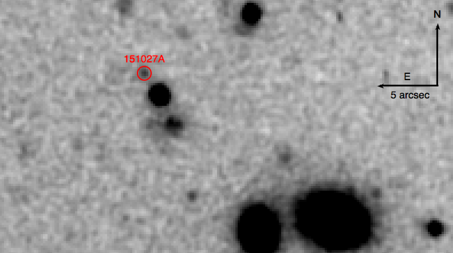
Figure 2: Finding chart obtained with the TNG observation at 19 days. The position of the optical afterglow of GRB 151027A is shown by the red circle. The bright extended source in the SW (Mazaeva et al. 2015; Dichiara et al. 2015) is also visible.

2.3 Radio data

Radio observations with the Very Large Array (VLA) 0.78 days after the trigger, performed at a mean frequency of 21.8 GHz, revealed a source with flux density of $\sim$1.7 mJy (Laskar et al. 2015). Subsequent Giant Meter Radio Telescope (GMRT) observations (Chandra et al. 2015) reported a detection most likely contaminated by a nearby bright unresolved source (P. Chandra - private communication).

We triggered an approved proposal with the Medicina 32m radio telescope and obtained ToO observations with the European VLBI Network (EVN), the Very Long Baseline Array (VLBA), and the 64m Sardinia Radio Telescope (SRT, Bolli et al. 2015; Prandoni et al. in prep.). Details of the data acquisition and reduction are given below. Results of the radio observations are listed in Table 1.

2.3.1 European VLBI (EVN) observations

We observed GRB 151027A with the European VLBI Network on 2015 November 18 and 2016 March 15. The participating stations were Effelsberg (100 m), Medicina (32 m), Torun (32 m), Yebes (40 m), Westerbork (25 m), Onsala (25 m), and Jodrell Bank (25 m). The observing frequency was centred at 4.98 GHz, with $8\times 16$ MHz baseband channels, in dual polarization.

Data were electronically transferred to the central correlator at JIVE via the so-called e–VLBI technique and processed in real time with the software correlator SFXC (Szomoru 2008; Keimpema et al. 2015). We observed in phase reference mode, alternating 1-minute scans on the nearby ($d=0.5^{\circ}$) calibrator J1806+6141 to 2.5-minute scans on the target for a total integration time on target of $\sim 4.2$ hours. We also regularly observed the two check sources J1815+6127 ($d=0.7^{\circ}$) and J1746+6226 ($d=3.0^{\circ}$). We carried out a standard calibration in AIPS, determining amplitude coefficients from gain curves and system temperatures recorded during the observation. We removed phase offsets and phase delays and rates using the phase calibrator J1806+6141. Phase solutions were then transferred to the target. After applying the calibrations, we produced a dirty image of the sky which immediately showed a point-like source. We then cleaned the image.

For the 2015 November observations, we achieve a noise level of 28 $\mu\mathrm{Jy\,beam}^{-1}$. A model-fit to the image plane with the AIPS task JMFIT yielded the following parameters for the source: RA 18h 09m 56.6965s $\pm 0.0001$s, Dec. +61^∘ $21\arcmin\ 13.1210\arcsec\pm 0.0002\arcsec$, peak brightness $(400\pm 50)$ $\mu\mathrm{Jy\,beam}^{-1}$. The component is unresolved, which implies a conservative upper limit to its size of about 1 milliarcsecond. The image is shown in Fig. 3

For the 2016 March observations, we achieve a noise level of $22\,\mu$Jy beam^-1, and the image plane model-fit results are RA 18h 09m 56.6965s $\pm$ 0.0001s, Dec. +61^∘ 21′13.1219″$\pm$ 0.0004″, peak brightness (125 $\pm$ 15) $\mu$Jy beam^-1.

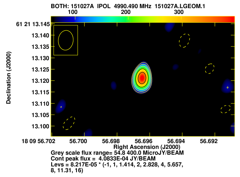
Figure 3: 5 GHz VLBI image of GRB 151027A taken with the EVN on 2015 November 18.

2.3.2 Very Long Baseline Array (VLBA) observations

We observed GRB 151027A with the Very Long Baseline Array (VLBA) 2016 Jan 24, Jan 30, and Feb 6. The observations were carried out at 5, 8, and 15 GHz, with a time partition given in Table 6. At each frequency, our set-up consisted of $8\times 32$ MHz baseband channels in dual polarization. We used the same calibrator–target scheduling pattern as in the EVN observations, with a duty cycle depending on the observing frequency (see Table 6). We carried out the standard calibration in AIPS, following the latest guidelines for VLBA amplitude calibration. We combined the DBCON data with the data from observations at the same frequency taken in different runs; no significant variability is expected on timescales shorter than a week. At 5 and 8 GHz, we clearly reveal a compact source at the image phase tracking centre determined from the EVN observations; we also detect the source at 15 GHz, but only if we use natural weights in the imaging process.

2.3.3 Medicina observations

We observed GRB 151027A with the 32m Medicina radio telescope on 2015 October 31. We observed with the Total Power backend at a central frequency of 24.5 GHz, with a bandwidth of 2 GHz. We performed 1043 cross-scans in right ascension and declination, centred on the position reported by Laskar et al. (2015). The total effective on-source time is 27 minutes. Data were calibrated with scans on NGC7027, and sky opacity was determined and compensated for through regular (about one per hour) skydip scans. No significant emission was detected above a 3 $\sigma$ noise level of 8.0 mJy.

2.3.4 Sardinia Radio Telescope (SRT) observations

We observed GRB 151027A with the 64m Sardinia radio telescope on 2015 October 30-31 between 23:30 UT and 01:30 at 22 GHz, and between 01:30 and 04:30 at 7.2 GHz. The observing strategy was based on cross-scans in azimuth and elevation directions, with the following parameters for each band: at 22 GHz we observed with a bandwidth of 2 GHz with a total of 242 scans for an effective on-source time of 5 minutes; at 7.2 GHz the bandwidth was 680 MHz with 336 scans and a net on-source time of 14 minutes. Owing to scheduling constraints, the observations took place at low elevation, between about 12^∘ and 19^∘. No significant emission was detected above a 3 $\sigma$ noise level of 6.0 mJy and 0.6 mJy respectively at the two frequencies. These values are dominated by the low elevation at high frequency and by confusion at low frequency.

Band	$t-t_{0}$ [s]	$F_{\nu}$ [mJy]	Ref.
1.4 GHz	$1.64\times 10^{6}$	0.312 $\pm\,$ 0.064	[1]
5 GHz	$1.92\times 10^{6}$	0.39 $\pm\,$ 0.05	[2]
5 GHz	$7.69\times 10^{6}$	0.29 $\pm\,$ 0.05	[3]
5 GHz	$1.20\times 10^{7}$	0.15 $\pm\,$ 0.03	[2]
7 GHz	$3.31\times 10^{5}$	$<0.6$	[4]
8.4 GHz	$7.95\times 10^{6}$	0.18 $\pm\,$ 0.03	[3]
15 GHz	$8.51\times 10^{6}$	0.14 $\pm\,$ 0.03	[3]
22 GHz	$6.74\times 10^{4}$	1.7	[5]
22 GHz	$3.31\times 10^{5}$	$<6.0$	[4]
24 GHz	$3.92\times 10^{5}$	$<8.0$	[6]

Table 1: Radio band fluxes and 3$\sigma$ upper limits used in this work.

[1] Chandra & Nayana (2015); [2] this work: EVN observations; [3] this work: VLBA observations; [4] this work: SRT observations; [5] Laskar et al. (2015); [6] this work: Medicina observations;

3 Data analysis and results

3.1 Prompt emission: First and second peaks

During the first two peaks of the light curve, corresponding to the time interval $\sim$0-24 seconds, we extracted three spectra: #1 and #2 corresponding respectively to the rise and decay phase of the first peak and #3 for the entire duration of the second (dimmer) peak (referring to the labelled regions in the middle panel of Fig. 1). We jointly fit the Fermi/GBM (NaI and BGO) and the Swift/BAT spectra with a cutoff power law model (CPL) with a free normalization constant between Fermi and Swift. Start and stop times and the best fit parameters (with 68% confidence errors) and the $\chi^{2}$(dof) are given in Table 2. Spectrum #3 can be fitted only with a simple power law model (i.e. the $E_{\rm peak}$ of the cutoff power law model is unconstrained). These three spectra are shown in the top panels of Fig. 1 where the data (green and red for the GBM and BAT, respectively) and the best fit model (solid black line) are shown.

Dataa	#	startb	stopb	Modelc	$\Gamma$	$E_{\rm peak}$	Ad	kT	ABB	$\chi^{2}$(dof)	P${}^{\rm F-test}_{CPL-CPLBB}$
		s	s			keV	ph cm-2 s-1	keV	ph cm-2 s-1
B+G	1	-0.256	1.792	CPL	0.92${}^{+0.08}_{-0.08}$	207${}^{+29}_{-23}$	2.93${}^{+0.84}_{-0.68}$	-	-	164(244)	-
…	2	1.792	6.912	CPL	1.29${}^{+0.15}_{-0.13}$	69${}^{+16}_{-6}$	6.09${}^{+2.84}_{-1.38}$	-	-	192(272)	-
…	3	17.152	23.296	PL	1.82${}^{+0.08}_{-0.08}$	-	9.43${}^{+3.26}_{-2.43}$	-	-	168(286)	-
X+B+G	4	90	100	CPL+BB	1.26${}_{-0.05}^{+0.04}$	218${}_{-59}^{+103}$	0.71${}_{-0.10}^{+0.09}$	1.23${}_{-0.19}^{+0.33}$	0.041${}_{-0.008}^{+0.009}$	211(256)	3.8$\times 10^{-7}$
…	5	100	110	CPL+BB	1.06${}_{-0.02}^{+0.02}$	316${}_{-41}^{+51}$	0.89${}_{-0.06}^{+0.06}$	3.02${}_{-0.20}^{+0.21}$	0.17${}_{-0.02}^{+0.02}$	279(301)	8.0$\times 10^{-13}$
…	6	110	120	CPL+BB	1.18${}_{-0.03}^{+0.02}$	209${}_{-22}^{+27}$	2.08${}_{-0.16}^{+0.16}$	2.01${}_{-0.08}^{+0.07}$	0.55${}_{-0.04}^{+0.05}$	257(296)	6.3$\times 10^{-35}$
…	7	120	130	CPL+BB	1.50${}_{-0.06}^{+0.05}$	76${}_{-14}^{+22}$	2.71${}_{-0.37}^{+0.37}$	1.12${}_{-0.06}^{+0.07}$	0.51${}_{-0.03}^{+0.03}$	284(293)	8.7$\times 10^{-45}$
X	8	130	140	BB	-	-	-	$0.63^{+0.02}_{-0.02}$	$0.25^{+0.01}_{-0.01}$	39(34)	-
…	9	140	150	PL+BB	$1.53^{+0.27}_{-0.38}$	-	$1.19^{+0.40}_{-0.47}$	$0.43^{+0.04}_{-0.03}$	$0.087^{+0.015}_{-0.013}$	30(26)	2.3$\times 10^{-6}$
…	10	150	160	PL+BB	$2.07_{-0.23}^{+0.19}$	-	$0.86_{-0.21}^{+0.18}$	$0.37_{-0.03}^{+0.03}$	$0.037_{-0.005}^{+0.006}$	36(46)	4.6$\times 10^{-10}$
…	11	160	170	PL	$2.53_{-0.06}^{+0.06}$	-	$1.19_{-0.04}^{+0.04}$	-	-	53(45)	(0.02)e
…	12	170	180	PL	$2.45_{-0.06}^{+0.07}$	-	$1.01_{-0.04}^{+0.04}$	-	-	50(40)	(0.01)e
…	13	180	190	PL	$2.65_{-0.08}^{+0.09}$	-	$0.76_{-0.03}^{+0.09}$	-	-	16(30)	-
…	14	190	200	PL	$2.51_{-0.10}^{+0.10}$	-	$0.57_{-0.03}^{+0.03}$	-	-	25(22)	-
XMM		7.8$\times 10^{5}$	1.3$\times 10^{6}$	PL+BB	$2.09^{+0.03}_{-0.04}$	-	$3.8^{+0.1}_{-0.2}\times 10^{-4}$	$0.11^{+0.03}_{-0.02}$	$3.1^{+2.0}_{-1.1}\times 10^{-6}$	398(345)	5.8$\times 10^{-7}$

Table 2: Prompt emission time resolved spectral analysis. ^aSpectral data used in the fit: B=Swift/BAT, G=Fermi/GBM and X=Swift/XRT. ^bTimes refer to the trigger time of the burst. ^cModels adopted in the fit: CPL=powerlaw with exponential cutoff, PL=powerlaw, BB=blackbody; galactic ($N_{\rm H,gal}$=3.7$\times$10²⁰ cm^-2) and intrinsic ($N_{\rm H}$=4.4$\times$10²¹ cm^-2) absorption is present in all models (using Tuebingen–Boulder ISM absorption model, Wilms et al. 2000). ^dSpectral normalization is computed at 1 keV. ^eIn this case the addition of a BB component is not statistically significant, as suggested by the value of the null hypothesis probability associated with the F–test. The horizontal lines correspond to the differently shaded regions in Fig. 1

3.2 Evidence of a thermal component: Third peak

The third peak of the light curve was observed by BAT and GBM above 10 keV and simultaneously by XRT in the 0.5 – 10 keV energy range. The light curves (see middle panel of Fig. 1) show that the XRT peak is delayed with respect to that observed by BAT and GBM. We selected four time intervals (from 90 s to 130 s after the trigger) where the data from three instruments overlap, and jointly fitted the spectra. This allows us to perform a time resolved spectral analysis over a wide energy range, namely from 0.5 keV to a few MeV.

We fit the spectra with a CPL model. Since the data extend down to 0.5 keV, it is necessary to take into account the galactic and intrinsic absorption. The Tuebingen–Boulder ISM absorption model (Wilms et al. 2000) encoded in the tbabs and ztbabs models of XSPEC is used. We assume the galactic absorption $N_{\rm H,gal}=3.7\times 10^{20}$ cm^-2 and keep it fixed, and we also allow for an intrinsic (at $z$=0.81) absorption. Also in this case we allow a free normalization constant between the Swift/BAT spectrum and the Fermi/GBM (NaI+BGO) spectra. In all the fits we find that this constant is within a factor of 2 and is consistent with 1.0.

If the intrinsic $N_{\rm H}$ is treated as a free parameter, we find that it varies dramatically (by more than one order of magnitude) describing a peak over a 30-second timescale coincident with the flare. We interpret this non-physical feature as being indicative of the possible presence of an additional component during the flare. We therefore fixed the intrinsic $N_{\rm H}$=0.44$\times 10^{22}$ cm^-2 which is the value found by fitting the XRT spectra at very late times (i.e. $>$5 days).

By visual inspection of the fitted spectra and their residuals we noticed systematic deviation from the model in the XRT 0.5-10 keV energy range, making the CPL fit unacceptable. We therefore tried to model this excess by adding the simplest two-parameter thermal blackbody (BB) component. We refitted the data and compared the new fit (i.e. absorbed cutoff power law plus blackbody – CPL+BB) with the old one (i.e. absorbed CPL) through an F–test. We find that in all of the four spectra describing the third emission episode of GRB 151027A there is statistically significant evidence for the presence of a thermal blackbody component. The probability of the F–test (representing the probability that the fit is not significantly improved by the additional BB component) is given in Table 2, along with the spectral parameters of the CPL+BB fit. The four spectra are shown in the bottom panels of Fig. 1.

The addition of the BB component to the CPL is the minimal assumption that can produce a curvature of the spectrum which adapts to the data points. However, we also verified whether the systematic deviation of the data from a simple CPL could also be accommodated by a second CPL. In order to have a similar number of free parameters of the BB, in this case we fixed the second CPL low energy photon index to the value predicted for single electron synchrotron emission, i.e. 2/3. In spectra #3 and #4, when the peaked component is less dominant, the fits performed using CPL+CPL or CPL+BB are statistically equivalent. Afterwards, when the component at low energies represents a considerable fraction of the total flux, the CPL+BB model is statistically preferable.

3.3 X–ray emission in the interval 130–200 seconds

After 130 s, the GBM and BAT data cannot be used for the spectral analysis. We analyse seven XRT spectra (corresponding to regions 8–14 in the middle panel of Fig. 1) in the time interval 130–200 s and fit with an absorbed power law (PL) or an absorbed power law plus a blackbody component (PL+BB). Given the limited energy range 0.5–10 keV we cannot determine the peak of a possible cutoff power law model. For each spectrum the statistical significance of the addition of the thermal component has been estimated through the F–test. For spectrum #8 the best fit is obtained with a pure BB model since the addition of a power law component does not constrain the power law fit parameters. In the following spectra the best fit model is PL+BB, in which the thermal component remains statistically significant up to 160 s. After that, the spectrum is best fitted by a single PL component.

The evolution of the spectral parameters is shown in Table 2 and Fig. 4.

Figure 4: Spectral evolution of GRB 151027A parameters through the entire burst duration. Panel (a) shows the temporal evolution of the non-thermal component spectral index. Panel (b) shows the evolution of the peak energy when the non-thermal component is described by a CPL. Panel (c) shows the BB temperature evolution. The last panel (d) shows the comparison between the fluxes, integrated in the 0.3–10 keV energy range, associated with the thermal (squares) and non-thermal component (points). The colour codes of the different symbols corresponds to the spectral data sets (the same colour coding) shown in Fig.1.

The results of the BAT-GBM-XRT spectral fits were compared with the optical $R$ band detection at 126 s (Pozanenko et al. 2015). The optical detection is compatible with the low energy extrapolation of the model (Fig. 5). This result suggests that the early optical emission could be produced by the same mechanism responsible for the high energy emission and therefore it should not be interpreted as standard afterglow.

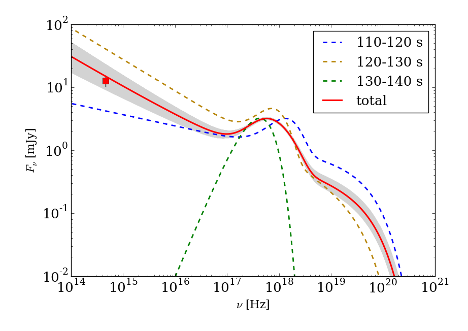
Figure 5: Comparison between the optical $R$ band detection at 126 s (red square, Pozanenko et al. 2015) and the fit of the composite XRT-BAT-GBM spectrum (red solid line). The grey shaded area represents the 1$\sigma$ scatter from the best fit.

3.4 XMM-Newton late time spectrum

The XMM-Newton late time spectral analysis was intended to obtain a more accurate estimate of intrinsic $N_{\rm H}$. We initially performed the fit using a PL model with free intrinsic absorption. From the residual, we noticed that a peaked component should be added to improve the fit. For this reason we refit the spectrum using a PL+BB model with free absorption. The XMM-Newton spectrum showed a still statistical significant thermal component that contributes to only $\sim$8% of the 0.3–10 keV flux. The BB temperature was lower than the one obtained from XRT spectrum # 10 (the last time interval where BB was detected). All the fit parameters are listed in Table 2.1.

The best fit $N_{\rm H}$ parameter obtained in the PL+BB model is fully compatible with the value obtained by the late time XRT spectrum.

The 0.3–10 keV flux corrected by intrinsic and galactic absorption is compatible with the flux measured by XRT at that time and it is shown by the light blue diamond in Fig. 6.

3.5 Radio

As an example of the VLBI data quality, we show in Fig. 3 the EVN image at 5 GHz obtained on 2015 Nov 18. We give in Table 7 (see Appendix A) the basic parameters (noise $\sigma_{\nu}$, peak surface brightness $B_{\nu}$, peak-to-noise ratio, and image resolution) of this and the other images; in Col. 7 we list the total flux density $S_{\nu}$ obtained from a visibility model–fitting carried out in Difmap. Estimating the accuracy of the amplitude scale for VLBI data is traditionally a difficult task. From an inspection of the data quality and of the calibrator images, and taking into account the local noise, we conservatively estimate it to be within 20%.

From the comparison of the EVN and the VLBA 5 GHz data, we find that the source flux density decreased by nearly 50% from day 22 to day 89, and by a further $\sim 50\%$ between day 89 and 140. Moreover, from the comparison of the nearly simultaneous VLBA multi–$\lambda$ data, we determine that the emission region is optically thin, with a spectral index of about $\beta=0.7-0.9$, assuming $F_{\nu}\sim\nu^{-\beta}$ (see fourth panel of Fig. 7).

The position of the source is consistent among the various experiments to within about 1 milliarcsecond. The mean coordinates are r.a. 18h 09m 56.6964s, dec. $+61^{\circ}\ 21\arcmin\ 13.1210\arcsec$. A more accurate astrometric calibration is beyond the scope of the present paper.

3.6 Afterglow light curve and spectral energy distributions

The XRT 0.3–10 keV unabsorbed flux, the $R$ band observations (see Tab. 5) and the radio detections and upper limits (see Tab. 1) were used to build the multiwavelength light curve of the afterglow of GRB 151027A shown in Fig. 6.

We built four spectral energy distributions at different times (1000 s, $1.8\times 10^{4}$ s, $6\times 10^{4}$ s, $7.7\times 10^{6}$ s) combining the data collected from GCNs, UVOT, and XRT observations and also radio VLBA observations. The unabsorbed fluxes are included in Tab. 3 and the four SEDs are shown in Fig. 7.

$\nu$ [Hz]	$F_{\nu}$ [mJy]	$\beta$	$t_{\rm c}$ [s]	Ref.
$5.55\times 10^{14}$	7.98 $\pm\,$0.66	–	1109	[1]
$6.93\times 10^{14}$	5.53 $\pm\,$0.25	–	1034	[1]
$8.57\times 10^{14}$	5.28 $\pm\,$0.19	–	893.4	[1]
$1.14\times 10^{15}$	2.48 $\pm\,$0.18	–	1072	[1]
$1.34\times 10^{15}$	1.66 $\pm\,$0.14	–	1130	[1]
$1.48\times 10^{15}$	1.66 $\pm\,$0.14	–	1086	[1]
XRT	$4.9\times 10^{-10}$	$1.23^{+0.11}_{-0.10}$	993	[2]
$3.72\times 10^{14}$	1.08 $\pm\,$0.039	–	$1.89\times 10^{4}$	[3]
$4.56\times 10^{14}$	1.89 $\pm\,$0.087	–	$1.89\times 10^{4}$	[3]
$6.32\times 10^{14}$	0.851 $\pm\,$0.047	–	$1.89\times 10^{4}$	[3]
XRT	$4.3\times 10^{-11}$	$1.31^{+0.10}_{-0.12}$	$1.84\times 10^{4}$	[2]
$2.19\times 10^{10}$	1.7	–	$6.74\times 10^{4}$	[4]
$1.37\times 10^{14}$	0.600 $\pm\,$0.055	–	$6.34\times 10^{4}$	[5]
$1.84\times 10^{14}$	0.658 $\pm\,$0.061	–	$6.26\times 10^{4}$	[5]
$2.46\times 10^{14}$	0.450 $\pm\,$0.042	–	$6.09\times 10^{4}$	[5]
$3.72\times 10^{14}$	0.297 $\pm\,$0.027	–	$6.58\times 10^{4}$	[5]
$4.56\times 10^{14}$	0.311 $\pm\,$0.034	–	$6.35\times 10^{4}$	[6]
$6.74\times 10^{14}$	0.258 $\pm\,$0.024	–	$6.46\times 10^{4}$	[5]
XRT	$3.5\times 10^{-12}$	$1.24^{+0.18}_{-0.10}$	$6.35\times 10^{4}$	[2]
$5.0\times 10^{9}$	0.29 $\pm\,$ 0.05	–	$7.69\times 10^{6}$	[7]
$8.4\times 10^{9}$	0.18 $\pm\,$ 0.03	–	$7.69\times 10^{6}$	[7]
$1.5\times 10^{10}$	0.14 $\pm\,$ 0.03	–	$7.69\times 10^{6}$	[7]

Table 3: Afterglow spectral energy distributions of GRB 151027A. For the XRT data the 0.3–10 keV flux in erg/cm²/s is shown in addition to the spectral slope $\beta$.

[1] this work: UVOT observations; [2] XRT automatic analysis (http://www.swift.ac.uk/xrt_products/00661775); [3] Yano et al. (2015); [4] Laskar et al. (2015); [5] Cano (2015); [6] Oksanen et al. (2015); [7] this work: VLBA observations.

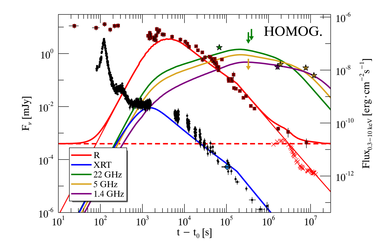
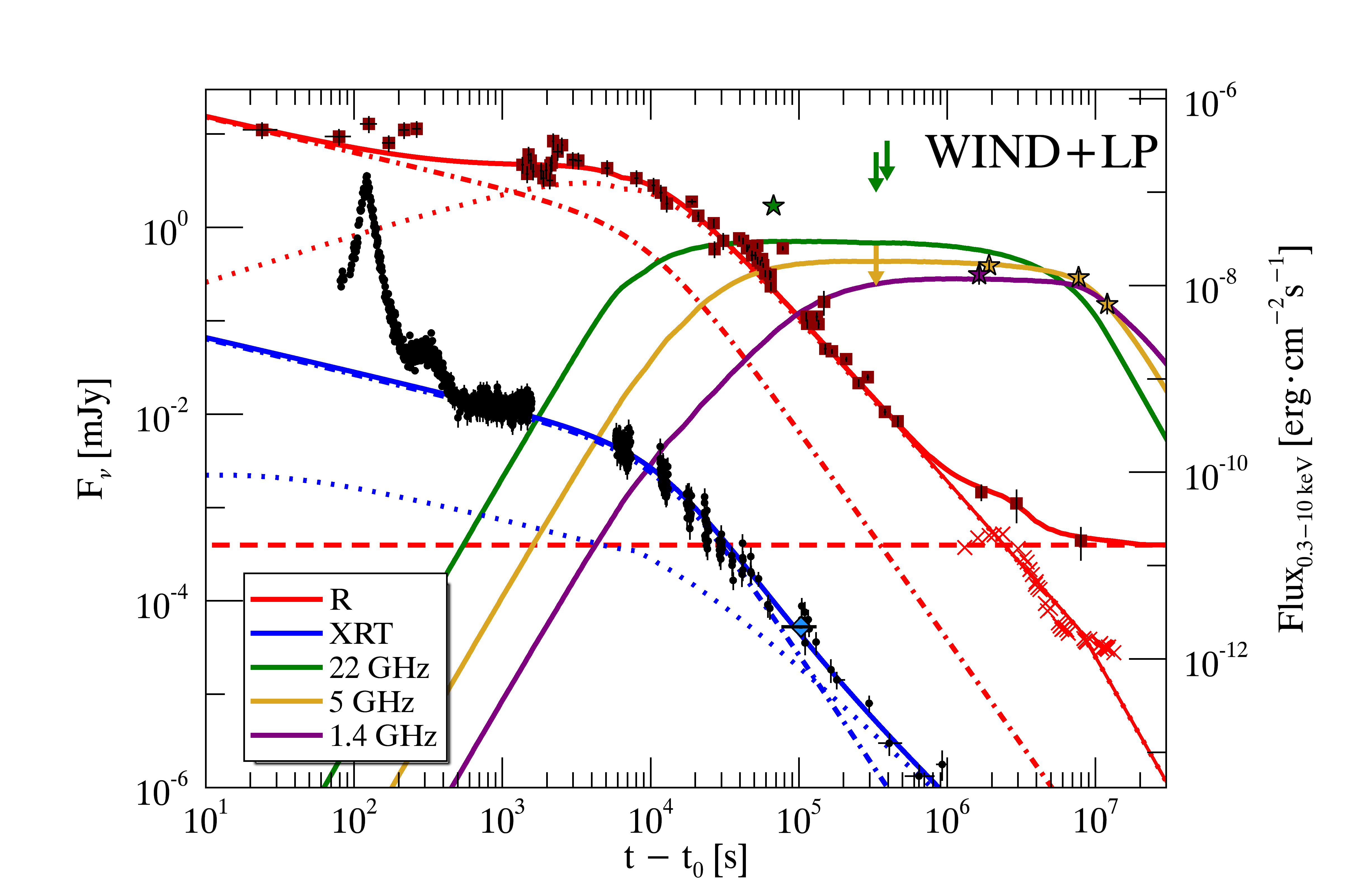
Figure 6: Multiwavelength light curve of the afterglow of GRB 151027A: XRT flux in band 0.3–10 keV (black circles, blue solid lines referring to the right y–axis), $R$ band flux density $F_{\nu}$ (red squares, red solid lines), 22 GHz (green star, green solid lines), 5 GHz radio detections and upper limits (orange stars, orange solid lines) and 1.4 GHz (purple star, purple solid lines). The light blue diamond shows the 0.3–10 keV flux measured by XMM-Newton. The red crosses represent a supernova light curve template obtained by shifting the light curve of SN1998bw at $z$=0.81 (Galama et al. 1998; Clocchiatti et al. 2011). The red dashed line shows the estimated $R$-band flux density of the host galaxy inferred from the LBT observation 92 days after the trigger. The 7 GHz SRT upper limit is shown in orange and compared with the 5 GHz model. The 24 GHz Medicina upper limit is shown in green and compared with the 22 GHz model. Top: Best afterglow modelling with a homogeneous external medium. Bottom: Best solution in the wind medium scenario in addition to a late prompt component. Dotted red and blue lines represent the afterglow forward shock emission in the $R$ and XRT band, respectively. Dash-dotted lines represent the late prompt component.

Figure 7: Spectral energy distributions of the afterglow of GRB 151027A. The four epoch data are collected in Tab. 3. The grey dashed lines represent the prediction of the model with external homogeneous medium density profile. The grey solid lines represent the prediction of the model with wind medium and late prompt. The afterglow component SEDs are shown by the dash-dotted lines (for the wind medium profile), while the late prompt component is shown by the dotted lines. The red long-dashed lines in the second and third panels show the best synchrotron spectrum compatible with the SEDs. The yellow regions show the possible positions of the cooling frequency $\nu_{\rm c}$.

4 Discussion

4.1 Prompt emission and flare

The prompt light curve of GRB 151027A shows three isolated emission peaks. The first two peaks have a standard behaviour with non-thermal spectra both characterized by a hard to soft evolution.

The third peak shows a statistically significant BB component at low energies superimposed on a cutoff power law. Evidence of a thermal emission have also been found in other GRB spectra. Typically it has been detected in the early phases of the prompt emission (Ghirlanda et al. 2003) or it can be present throughout the entire burst duration (Ryde 2004; Bosnjak et al. 2006; Ghirlanda et al. 2013) and it has been detected in X–ray flares (Peng et al. 2014). Furthermore, Starling et al. (2012) and Sparre & Starling (2012) have presented systematic research of thermal signatures in X–ray emission. According to the classification of Ghirlanda et al. (2013), GRB 151027A belongs to Class III of the thermal bursts because the thermal and non-thermal components coexist. Fig. 8 shows the simultaneous evolution of the 0.3–1000 keV and 0.3–10 keV luminosity of the two components.

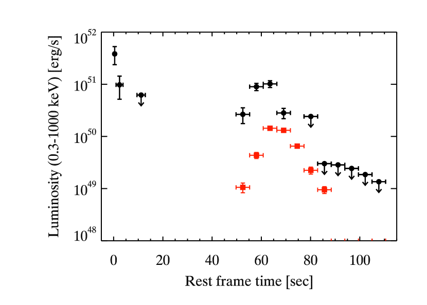
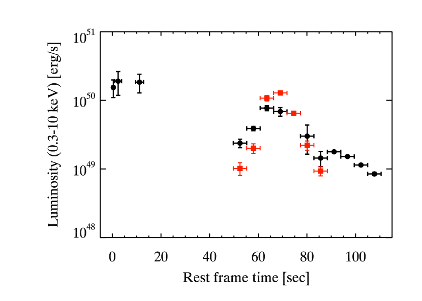
Figure 8: Top: 0.3–1000 keV luminosity as a function of rest frame time divided into thermal (red squares) and non-thermal component (black circles). Upper limits to the non-thermal luminosity are shown when the peak energy of the cutoff powerlaw component is not constrained. Bottom: Same as the top, but for luminosity in the range 0.3–10 keV.

The X–ray flare of GRB 151027A has a very luminous thermal component ($\sim$10⁵⁰ erg s^-1 near the peak) characterized by a low temperature ($kT_{\rm BB}\sim 1$ keV, a factor of $\sim$10 lower than the typical temperature observed in GRB prompt emission, e.g. Ryde 2004). Furthermore, the thermal luminosity peaks later than the non-thermal component and, at its maximum, it contributes to most of the total luminosity in the 0.3–10 keV and to 35% of the 0.3–1000 keV luminosity. In addition, the thermal component is still detected in the XMM-Newton late time spectrum with a luminosity $\sim$5$\times 10^{44}$ erg s^-1, corresponding to $\sim$8% of the 0.3–10 keV emission. In the following, we discuss the possible origin of this blackbody emission.

The hypothesis that the observed blackbody emission is due to a Ib/c SN shock breakout has to be excluded. In fact, the typical X–ray luminosity of such emission is $\sim$10⁴⁵ erg s^-1 (see e.g. Matzner & McKee 1999; Campana et al. 2006; Ghisellini et al. 2007c), which is much lower than the BB luminosity ($\sim$10⁵⁰ erg s^-1) observed at the peak of the flare in GRB 151027A.

Piro et al. (2014) proposed a model based on the emission of a hot plasma cocoon (based on Pe’er et al. 2006) to explain the long-lasting thermal emission observed in the ultra-long GRB 130925A. Starling et al. (2012) also used the cocoon expansion to explain the presence of thermal emission in X–ray spectra of GRB associated with a SN explosion. Even this model cannot be applied to our case because the peak luminosity reached by the thermal component during the flare is larger than the expected value (which is of the order of $10^{47}$ erg s^-1 or greater).

Thermal emission is naturally predicted within the standard fireball scenario, when the relativistically expanding fireball releases the internal photons at the transparency radius (e.g. Goodman 1986; Paczynski 1986; Daigne & Mochkovitch 2002). Owing to the initial huge opacity of the fireball (optical depth $\tau\gg 1$), photons can reach the thermodynamic equilibrium and are characterized by a BB spectrum.

Using the observables associated with the BB spectrum, i.e. the temperature $kT_{\rm BB}$ and the flux $F_{\rm BB}$, we can estimate the fundamental parameters of the fireball (see Ghirlanda et al. 2013). We can first obtain the ratio between the radius of the fireball and its bulk Lorentz factor $R_{\rm T}/\Gamma_{\rm T}$ when it becomes transparent:

$$\frac{R_{\rm T}}{\Gamma_{\rm T}}=2.406\frac{d_{\rm L}(z)}{(1+z)^{2}}\left(\frac{F_{\rm BB}}{\sigma T_{\rm BB}^{4}}\right)^{1/2}{\rm cm}$$ (1)

The evolution of this ratio during the third emission peak is shown in Fig. 9.

In order to test this hypothesis further, we need to make an assumption about when transparency occurs:

(i) It might happen during the acceleration phase when, owing to the high internal pressure, the fireball is still accelerating, converting its internal energy to bulk motion energy. In this case, it is possible to estimate the distance from the central engine $R_{0}$, where the fireball is created, assuming an initial bulk Lorentz factor $\Gamma_{\rm i}=1$. We obtain $R_{0}\sim 10^{11-12}$ cm.

(ii) It might happen during the coasting phase. The internal pressure is no longer sufficient to accelerate the fireball that proceeds with constant bulk Lorentz factor. In this case combining Eq. 1 with the relations shown in Daigne & Mochkovitch (2002) we can obtain $R_{\rm T}$, $\Gamma_{\rm T}$, and $R_{0}$. Differently from the previous case, these values are not unequivocally determined because they depend on the blackbody radiative efficiency $\eta_{\rm BB}$. As in Ghirlanda et al. (2013) we use a radiative efficiency related to the thermal component of about $\eta_{\rm BB}\sim 10^{-2}$, since the blackbody flux varies from $\sim 5\%$ up to $\sim 50$% of the non-thermal flux. Then, we find $R_{\rm T}=10^{13-14}$ cm, $\Gamma_{\rm T}\sim 60$, and $R_{0}\sim 10^{9-10}$ cm (Fig. 10).

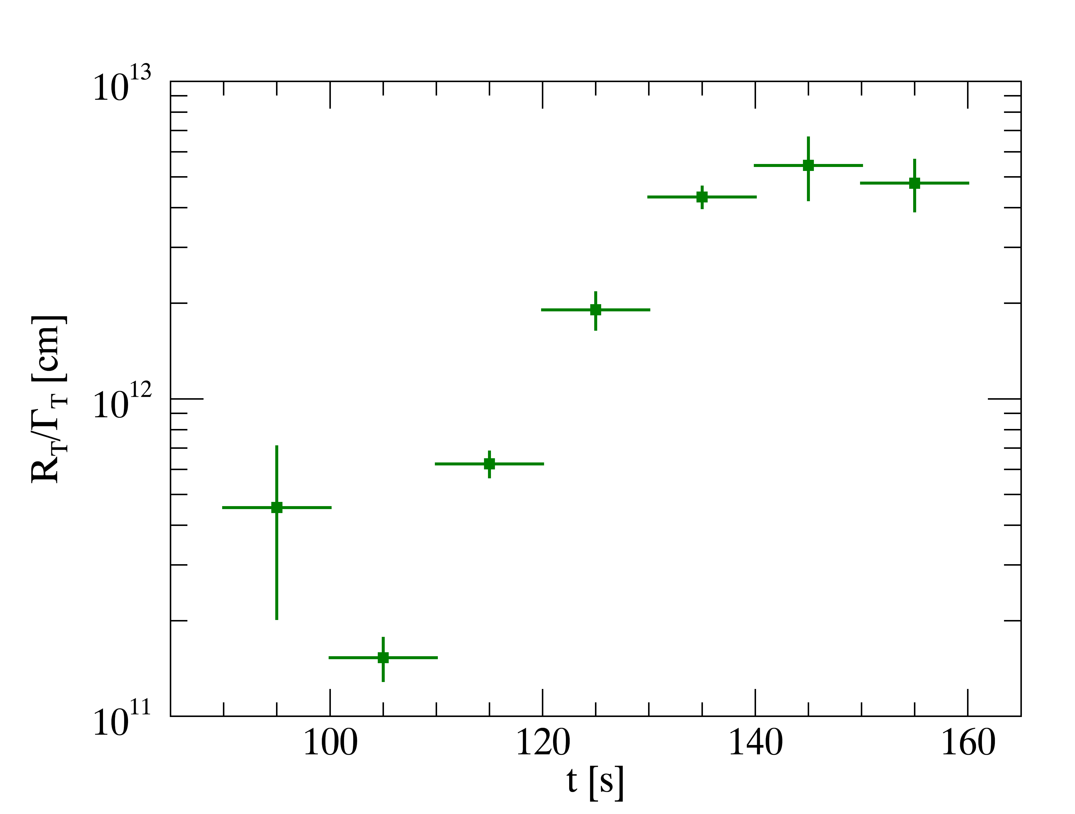
Figure 9: $R_{\rm T}/\Gamma_{\rm T}$ as a function of time obtained by the fit of time resolved spectra of the flare (Eq. 1).

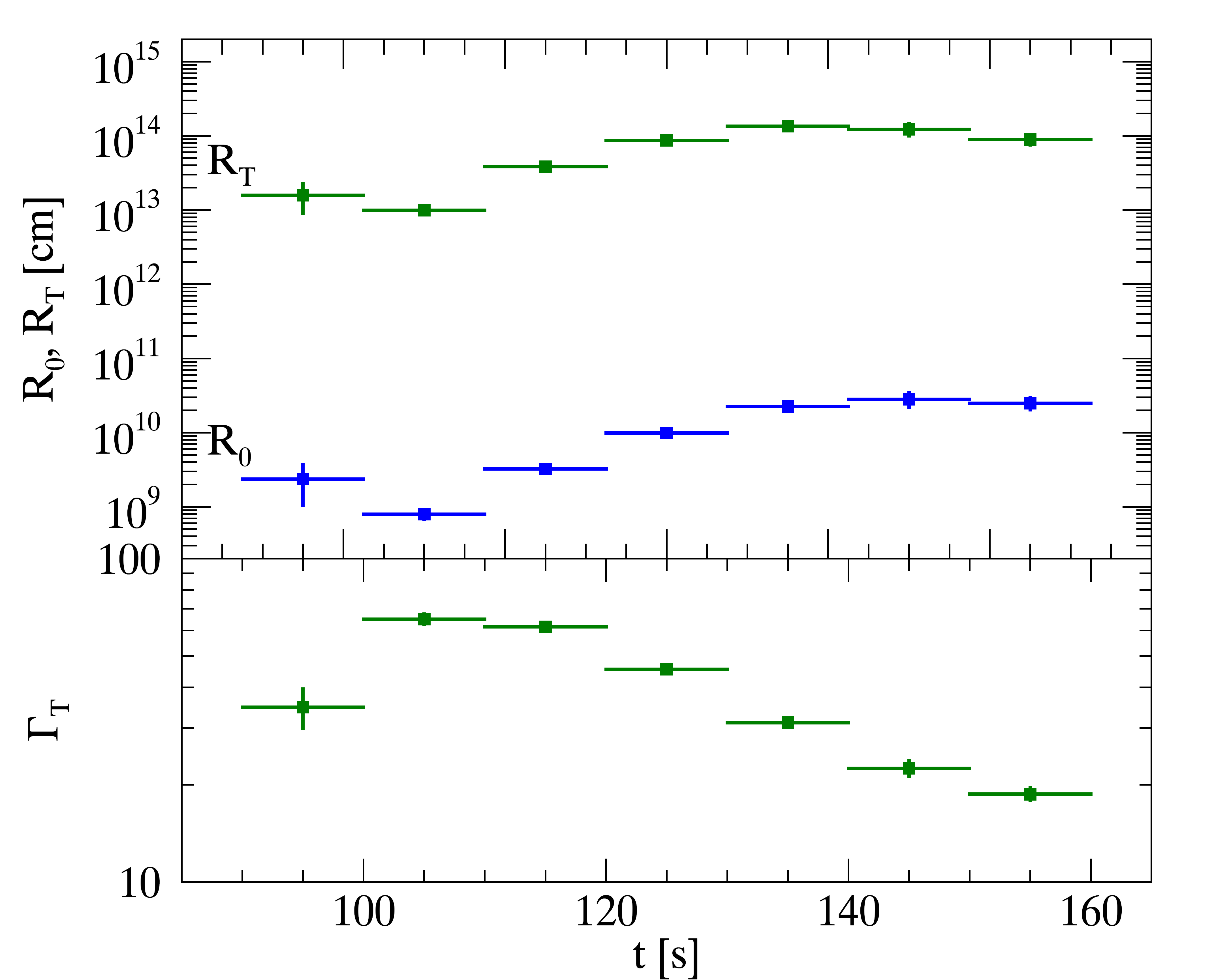
Figure 10: $R_{\rm T}$, $\Gamma_{\rm T}$, and $R_{0}$ as functions of time in the hypothesis that the fireball becomes transparent during the coasting phase. In this case we used $\eta_{\rm BB}=10^{-2}$.

In both cases the value of $R_{0}$ is much higher than expected. Assuming that the progenitor of long GRBs is a newly born compact object (a black hole or a magnetar) produced by the core collapse of a Wolf–Rayet star (Usov 1992; Duncan & Thompson 1992; Woosley 1993; MacFayden & Woosley 1999), we can suppose that the fireball should be formed near the central object, at a few gravitational radii. For a compact object of $5-10\,M_{\odot}$, the gravitational radius is $\sim 10^{6}$ cm, so we expect that $R_{0}\sim 10^{7}$ cm, a value much smaller than the obtained one.

In case (ii), the value we should use for $\eta_{\rm BB}$ in order to get $R_{0}\sim 10^{7}$ is $\sim 10^{-4}$. Such a low radiative efficiency would imply an enormous burst of kinetic energy. Therefore, we expect a very energetic afterglow that is in contrast with what we observe.

Another possible explanation of the significant thermal emission of GRB 151027A is given by the “reborn fireball” model (Ghisellini et al. 2007a). In this scenario the thermal emission is produced by plasma heated in the collision between the relativistic ejecta and the surrounding material released by the progenitor star during its final evolution stages.

If the optical depth after collision is large, a re-acceleration to relativistic speed due to the dissipated internal energy can take place. This process allows the creation of a reborn fireball with a larger initial radius $R_{0}\sim 10^{11}$ cm consistent with the large values inferred for GRB 151027A.

Ghisellini et al. (2007a) assume the target material to be at rest with respect to the central engine. Nevertheless, in our case the relativistic shells that produced the first two prompt emission peaks should have interacted with such material first. For this reason, we must conclude that the optically thick target material was not there when the first prompt photons were emitted.

A possible way around this is to assume the GRB central engine itself is responsible for the production of the target material. At the beginning, shells that produce the initial part of the prompt emission are ejected. Then a denser and slower shell is ejected, which does not emit radiation since it is optically thick. After a quiescent period a quicker shell is ejected and it reaches the slower one. In this scenario the reborn fireball is actually like an internal shock between a thick, mildly relativistic, massive shell with a quicker shell. The collision dissipates energy with non-negligible efficiency since the relative Lorentz factor can be large. The photons produced cannot escape because of the large opacity and the internal thermal energy can be used to re-accelerate the shell. Beyond the photospheric radius the shell emits the blackbody radiation produced by the reprocessing of the trapped photons and a non-thermal component. The decreasing emission of the flare is then due to the quenching of the radiation of the shell and to the off latitude emission.

4.2 Modelling the afterglow

In this section we propose a model for the afterglow light curve from the XRT 0.3–10 keV flux to the optical $R$ band and to the radio frequencies. As was said before, both the X–ray and optical early time flux (for $t_{\rm obs}\,\lower 3.22916pt\hbox{$\sim$}\hbox to0.0pt{\hss\raise 1.1625pt\hbox{$<$}}\,500$ s) is contaminated by the emission of the flare. For this reason, we focus on the observed light curves only for $t_{\rm obs}\,\lower 3.22916pt\hbox{$\sim$}\hbox to0.0pt{\hss\raise 1.1625pt\hbox{$>$}}\,500$ s. At this epoch, the X-ray light curve shows the presence of a plateau phase (Nousek et al. 2006), which is usually related to a late time central engine activity (see e.g. Zhang et al. 2006; Dai & Lu 1998; Zhang & Mészáros 2001; Kumar et al. 2008; Corsi & Mészáros 2009; Metzger et al. 2011; Leventis et al. 2014; van Eerten 2014; Duffell & MacFayden 2014). However, we first attempt to model the multiwavelength long-lasting emission of GRB 151027A as produced uniquely by the forward shock.

4.2.1 Model

The modelling of the observed afterglow light curves has been performed with a semi-analytic model that combines the forward shock dynamics developed in Nava et al. (2013) with the computation of the spectrum of the emitted radiation, based on Nappo et al. (2014), already used in Melandri et al. (2015). The model will be presented in more detail in a future paper in preparation. Here we introduce only the most relevant features.

We assume that the blastwave starts moving at relativistic velocity with an initial bulk Lorentz factor $\Gamma_{0}$, and with an initial kinetic energy $E_{\rm kin,0}$ that is linked to the emitted $\gamma$–ray isotropic energy $E_{\rm\gamma,iso}$ and the efficiency $\eta$ by

$$E_{\rm kin,0}=(1-\eta)E_{\rm\gamma,iso}/\eta$$ (2)

Then the fireball decelerates because of the interaction with the external medium and dissipates its energy (see Nava et al. 2013 for an exhaustive treatment). We assume that a fraction $\epsilon_{\rm e}$ and $\epsilon_{\rm B}$ of the dissipated energy is distributed to the leptons and the magnetic field, respectively. The remaining energy is given to protons. The energy is given to electrons with an energy distribution $Q(\gamma)\propto\gamma^{-p}$. The leptons can cool for synchrotron and synchrotron self-Compton (SSC) emitting a fraction $\epsilon_{\rm rad}$ of their total energy. At each time step we compute the following:

• the synchrotron spectrum in the optically thin and in the self-absorbed regime;

• the $Y$ Comptonization parameter;

• the SSC spectrum;

• the fraction $\epsilon_{\rm rad}$ of injected energy that is actually radiated.

The resulting spectrum is normalized at each time step to the bolometric luminosity obtained by the dynamical evolution. The fireball is assumed spherical, but it is possible to insert a jet break in the light curves when the beaming cone of width $1/\Gamma$ becomes larger than the jet opening angle $\theta_{\rm jet}$, which produces an achromatic steepening of the temporal index $\alpha$. We can describe the propagation of the forward external shock in a circumburst medium (CBM) with a generic density profile $n(R)$. In this work we will test only the two standard cases: homogeneous medium ($n(R)=$ const) and wind–medium ($n(R)\propto R^{-2}$); the first describes the density profile typical of the interstellar medium and the second describes the stratified density profile that can be produced by the intense stellar winds in the final stages of the Wolf–Rayet star evolution.

Parameter	Homogeneous CBM	Wind CBM
	($s=0$)	($s=2$)
$\Gamma_{0}$	125	48
$\epsilon_{\rm e}$	0.22	0.04
$\epsilon_{\rm B}$	$8\times 10^{-5}$	0.06
$n_{0}$	0.08 cm-3	$0.04\,A_{*}$
$\eta$	0.035	0.16
$p$	2.4	2.65
$\theta_{\rm jet}$	$4.2^{\circ}\$	$6.3^{\circ}\$
$E_{\rm\gamma}$ [erg]	$1.1\times 10^{50}$	$2.4\times 10^{50}$
$E_{\rm\gamma,iso}$ [erg]	$3.98\times 10^{52}$	$3.98\times 10^{52}$
Late Prompt Parameters
$T_{\rm A}\,[{\rm s}]$	–	$1\times 10^{5}$
$L_{\rm A}$ [erg/s]	–	$1.3\times 10^{46}$
$\nu_{\rm b}\,[{\rm Hz}]$	–	$1\times 10^{16}$
$\beta_{\rm X}$	–	$1.0$
$\beta_{\rm o}$	–	$0.6$
$\alpha_{\rm fl}$	–	$0.4$
$\alpha_{\rm st}$	–	$2.0$

Table 4: Parameters of GRB 151027A in the homogeneous and wind scenarios. The CBM density is expressed as $n(R)=n_{0}\times R^{-s}$, where $s=0$ represents the case of homogeneous CBM and $s=2$ the case of wind CBM, where the coefficient is expressed in unity of $A_{*}=3\times 10^{35}$ cm^-1. $L_{\rm A}$ is the 0.3–10 keV luminosity of late prompt at $T_{\rm A}$.

4.2.2 Homogeneous CBM scenario

The best result obtained using this modelling hypothesis is represented in the top panel of Fig. 6. The values used for the parameters in this scenario are given in the first column of Tab. 4. The solution was obtained using standard values except for the efficiency $\eta$, which is about an order of magnitude smaller than typical values ($\eta\sim 0.2$). In addition, a remarkably small value for $\epsilon_{\rm B}$ is used because, with a small magnetic field, the cooling frequency $\nu_{\rm c}$ is closer to the value inferred by the modelling of the $\sim$1.8$\times$10⁴s SED with a pure synchrotron spectrum (see yellow region in panel 2 of Fig. 7).

The injection index of the electrons $p=2.4$ is consistent with the slope of the optical spectrum $\beta_{\rm o}$ measured at $t\sim 6\times 10^{4}$ s ($\beta_{\rm o}=(p-1)/2\simeq 0.7-0.9$). Nevertheless, with this choice of $p$, a steepening of the light curve decay ($\Delta\alpha\sim 1$) for $t>2\times 10^{5}$ s is necessary to account for the optical and X–ray late time behaviour. We interpret this achromatic steepening as the jet break (Rhoads 1997; Sari et al. 1999). Using the standard relations for the jet break time in a homogeneous external medium (Sari et al. 1999) we can determine the jet opening angle $\theta_{\rm jet}$$=4.2^{\circ}$.

The collimation corrected $\gamma$-ray emission is $E_{\gamma}=E_{\rm\gamma,iso}(1-\cos\theta_{\rm jet})=1.1\times 10^{50}$ erg, where we used the isotropic energy obtained by Fermi–GBM integrated spectrum $E_{\rm iso}=3.98\times 10^{52}$ erg (cf. §2.1). This result has been compared with the $E_{\rm peak}-E_{\gamma}$ correlation (Ghirlanda et al. 2004, 2007) and the burst is $4\sigma$ off the best fitting line. Using the Fermi–GBM rest frame $E_{\rm peak}=615$ keV, the jet opening angle that would make the GRB consistent with the $E_{\rm peak}-E_{\gamma}$ correlation is $\theta_{\rm jet}=14^{\circ}$, which should have generated an achromatic break in the light curves at $t\sim 5.8\times 10^{6}$ s. No break is observed at this epoch.

Radio 5 GHz observations provide the main evidence that excludes the homogeneous model. Fig. 11 is a zoomed view of Fig. 6 in which the late time 5 GHz model predictions with both homogeneous and wind model are compared with the data. Indeed, the 5 GHz model in the homogeneous case is not compatible with the SRT upper limit at $3.5\times 10^{5}$ s and with the EVN and VLBA observations. This significant incompatibility, in addition to the lack of strong evidence of an achromatic break at $t\sim 2\times 10^{5}$ s, leads us to conclude that the homogeneous density profile does not provide a good modelling of the afterglow of GRB 151027A.

4.2.3 Wind CBM scenario

The best solution obtained in the wind CBM scenario is plotted in the bottom panel of Fig. 6. The corresponding parameters are shown in the second column of Table 4. We adopted standard values for the parameters, except for the density parameter $n_{0}$, which is a factor of 25 smaller than the typical value $A_{*}=\dot{M_{\rm w}}/(4\pi m_{\rm p}v_{\rm w})=3\times 10^{35}$ cm^-1 obtained for a mass loss rate $\dot{M_{\rm w}}=10^{-5}$ M_⊙ yr^-1 and a wind velocity $v_{\rm w}=1000$ km s^-1, typical of a Wolf–Rayet star (Chevalier & Li 1999, 2000).

The injection index $p=2.65$ is compatible with the optical spectral slope of the SED at $\sim 6\times 10^{4}$ s and allows a description of the optical light curve temporal decay, which is better than the value obtained in the homogeneous model.

The 22 GHz VLA observation at 0.78 days after the trigger (Laskar et al. 2015) deviates from the model prediction by a factor of $\sim 2.5$. This inconsistency can be explained with the scintillation caused by the circumburst medium (Goodman 1997), which should modulate the early radio flux of GRB afterglows. For example, in the case of GRB 970508 (Frail et al. 1997; Taylor et al. 1997) the early time observed radio flux is strongly modulated up to a factor of $\sim 4$ at 8.46 GHz.

The prediction for the X–ray afterglow flux (blue dotted line in the bottom panel of Fig. 6) is much lower than the observed value. Furthermore, the X–ray light curve profile shows some elements such as a plateau and a flare that cannot be explained in the standard forward shock scenario. For these reasons, to model the X–ray emission we need to introduce another component of different origin.

The presence of this extra component is also suggested by the SEDs of the afterglow, especially the $\sim$1000 s SED obtained with UVOT and XRT (first panel of Fig. 7). The X–ray flux is much higher than the extrapolation of the power law component of the UVOT emission and requires another component to be consistent. Instead, the single spectral energy distributions taken at $\sim$1.8$\times$10⁴ s and $\sim$6$\times$10⁴ s (panels 2 and 3 in Fig. 7) are compatible with standard synchrotron emission spectrum in slow cooling regime (i.e. the injection frequency is smaller than the cooling frequency, $\nu_{\rm i}<\nu_{\rm c}$; e.g. Panaitescu & Kumar 2000) produced by a leptonic population with injection index $p\sim 2.4-2.8$. Nevertheless, the cooling break frequency is required to evolve as $\nu_{\rm c}\propto t^{-1.7}$. Such evolution is incompatible with the standard scenario in both CBM density profiles and can be accounted for assuming a further component in X–rays evolving differently from the standard forward shock evolution (Blandford & McKee 1976; Granot & Sari 2002) that we generically address as late prompt component (Ghisellini et al. 2007b). This is generated by a long-lasting central engine activity that ejects other shells that can move at relativistic velocity, but with less energy and with a smaller Lorentz factor $\Gamma$. The physical mechanism that produces these shells relies on the nature of the central engine itself, is beyond the scope of the present work, and will not be discussed further. The modelling used for the late prompt component is taken from Ghisellini et al. (2009), in which

• the spectral shape is assumed to be constant in time and described by a broken power law:

  $$L_{\rm late}(\nu,t)=L_{\nu_{\rm b}}(t)\begin{cases}\left(\nu/\nu_{\rm b}\right)^{-\beta_{\rm o}}&\nu\leq\nu_{\rm b}\\ \left(\nu/\nu_{\rm b}\right)^{-\beta_{\rm X}}&\nu>\nu_{\rm b}\\ \end{cases};$$ (3)

• the temporal evolution follows a smoothly broken power law profile:

  $$L_{\rm late}(\nu,t)=L_{\rm late}(\nu,T_{\rm A})\frac{(t/T_{\rm A})^{-\alpha_{\rm fl}}}{1+(t/T_{\rm A})^{\alpha_{\rm st}-\alpha_{\rm fl}}};$$ (4)

• the late prompt emission is present only in the optical and X–ray bands. Between the radio and the optical frequencies and beyond the X-ray frequencies there are exponential cutoffs. The cutoff frequencies are not considered as free parameters of the model.

There are seven parameters needed to describe the late prompt component: $\beta_{\rm X}$, $\beta_{\rm o}$, and $\nu_{\rm b}$ for the spectral behaviour; $\alpha_{\rm fl}$, $\alpha_{\rm st}$, and $T_{\rm A}$ for the temporal evolution; and $L_{\rm A}=\int L_{\rm late}(\nu,T_{\rm A})\,{\rm d}\nu$ for the normalization over the 0.3–10 keV band. The late prompt parameters adopted for the modelling are shown in Tab. 4.

Figure 11: Zoom of the 5 GHz band late time light curve (see Fig. 6). Dashed line represents the homogeneous model and solid line represents the wind model. The 7 GHz SRT upper limit is compared with the 5 GHz model predictions.

Late time EVN and VLBA 5 GHz radio observations and the SRT 7 GHz upper limit are in remarkable agreement with the solution of the wind density profile. In particular the very flat evolution of the 5 GHz light curve (indicated by the SRT upper limit and the 5 GHz observation between $10^{6}$ s and $8\times 10^{6}$ s) can be explained with standard afterglow relations only in the case of a wind profile if the frequency of observation is between the self-absorption frequency $\nu_{\rm a}$ and the injection frequency $\nu_{\rm i}$.

The EVN observation of March 15 shows a very steep decrease in the 5 GHz flux that can be explained by the presence of a jet break between the observations of Feb 6 and Mar 15. Adopting a value of $t_{\rm j}=8\times 10^{6}$ s, the value of the jet angle can be estimated with standard relations (see e.g. Chevalier & Li 2000). We obtain $\theta_{\rm j}=6.3^{\circ}$, corresponding to a collimation corrected energy of $E_{\gamma}=2.4\times 10^{50}$ erg. The late time jet break is consistent with the low value of the density parameter that is inferred from the modelling. In fact, in a low density environment the fireball takes a longer time to decelerate and thus the bulk Lorentz factor $\Gamma$ becomes smaller than $\theta_{\rm jet}^{-1}$ at later times. In this case, the inferred value for $E_{\gamma}$ is fully consistent at 1.4$\sigma$ with the $E_{\rm peak}-E_{\gamma}$ correlation.

The compatibility with the $E_{\rm peak}-E_{\gamma}$ correlation can be considered as indirect evidence, in addition to the radio late time observations (Fig. 11), that lead us to conclude that the blastwave of GRB 151027A is expanding in a medium shaped by the wind of the stellar progenitor.

4.2.4 Possible evidence of SN?

Late time optical observations after 19 days show a flattening in the light curve that can be explained by the presence of a supernova and the host galaxy emission. At 33 days a bump is identified in the optical light curve and it has been compared with a template of SN emission, namely the light curve of SN1998bw (Galama et al. 1998; Clocchiatti et al. 2011) rescaled at $z=0.81$ (red crosses in Fig. 6). In particular, we synthesized the observed-frame $R$-band light curve of SN1998bw as it would appear if it occurred at that redshift using its rest-frame light curves and interpolating over frequency (Cano 2013; Melandri et al. 2014). We then included the SN contribution in the GRB late time light curve without applying any stretch (in flux or time). In Fig. 12 the late time $R$-band light curve already shown in Fig. 6 is zoomed and compared with the modelling without the supernova contribution. Although the model without the supernova component is not incompatible with the LBT observation at $2.8\times 10^{6}$ s, the presence of a supernova emission leads to a better agreement with the late time observations.

Figure 12: Zoom of the $R$-band late time light curve (see Fig. 6). On the left data are modelled with afterglow (solid lines for wind medium, dashed lines for homogeneous medium), host galaxy (dotted line), and supernova component (red crosses), on the right only with afterglow and host galaxy.

If confirmed, it would be the eighth most distant GRB/SN association ever discovered (see e.g. Hjorth & Bloom 2012; Cano et al. 2016). The last LBT observation at 92 days after the trigger suggests the presence of an additional component that we interpret as the emission of the host galaxy. In this case the estimated flux density of the host galaxy is $\sim$ 0.4 $\mu$Jy in the $R$ optical band ($R_{\rm AB}\sim 25$), similar to the flux density of other GRB host galaxies at the same redshift (e.g. Savaglio et al. 2009; Hjorth et al. 2012; Vergani et al. 2015; Perley et al. 2016). Only further observations (at least as deep as the LBT ones) can give a possible confirmation of this hypothesis.

5 Conclusions

GRB 151027A, the 999th GRB observed by Swift, is the first GRB with a bright flare starting $\sim$100 s after the GRB trigger and lasting $\sim$70 s, that has been simultaneously observed from the optical band up to the MeV $\gamma$-ray energy. The time resolved spectral analysis of this flare indicates the presence of a blackbody component that provides up to 35% of the total luminosity in the 0.3–1000 keV band.

In this work we discussed the possible origin of this thermal radiation. Since the radius and the luminosity of the blackbody emission were too large to be interpreted as the photospheric emission of a standard fireball model, we explored a reborn fireball scenario (Ghisellini et al. 2007a) in which the thermal radiation is produced by the energy dissipation due to the collision of a relativistic shell with a more massive, optically thick, slower one.

Intensive follow up campaigns provided a well-sampled multiwavelength afterglow light curve from X-rays to the radio band.

We interpreted the afterglow emission, where possible, in the standard forward shock scenario. We tested two CBM density profiles: the homogeneous (constant density, typical of the interstellar medium) and wind profile (with $n(R)\propto R^{-2}$, typical of the medium surrounding a massive star in the final stages of its evolution). Since the X–ray light curve showed a plateau that cannot be explained by a standard afterglow behaviour, we needed to add a late prompt component (Ghisellini et al. 2007b).

Late time radio observations provide direct evidence of the better agreement of the data with the wind density profile model. In this case a jet break is observed, corresponding to a jet angle $\theta_{\rm jet}=6.3^{\circ}$.

Late time optical observations highlighted the presence of a bump in the light curve that can be interpreted as a supernova signature. The late flattening of the $R$-band light curve allowed us to estimate the host galaxy flux $\sim$0.4 $\mu$Jy ($R_{\rm AB}\sim 25$).

Appendix A Additional tables

Table 5: Optical $R$–band light curve

$t-t_{0}$ [s]	$t_{\rm exp}$ [s]	$F_{\nu}$ [mJy]	Ref.	$t-t_{0}$ [s]	$t_{\rm exp}$ [s]	$F_{\nu}$ [mJy]	Ref.
24	12	11.08 $\pm$ 2.053	[1]	$3.949\times 10^{4}$	150	0.7666 $\pm$ 0.04238	[8]
79.2	30	9.388 $\pm$ 1.739	[2]	$4.195\times 10^{4}$	150	0.7187 $\pm$ 0.04637	[8]
126	30	12.84 $\pm$ 2.379	[2]	$4.457\times 10^{4}$	150	0.6033 $\pm$ 0.04449	[8]
171.6	30	8.027 $\pm$ 1.487	[2]	$4.520\times 10^{4}$	180	0.5967 $\pm$ 0.01649	[9]
217.2	30	11.08 $\pm$ 2.053	[2]	$4.609\times 10^{4}$	180	0.6283 $\pm$ 0.01736	[9]
264	30	11.39 $\pm$ 2.11	[2]	$4.822\times 10^{4}$	1200	0.5018 $\pm$ 0.05558	[10]
1366	30	4.705 $\pm$ 0.8716	[2]	$5.077\times 10^{4}$	1200	0.5018 $\pm$ 0.04165	[10]
1468	30	3.737 $\pm$ 0.6923	[2]	$5.242\times 10^{4}$	150	0.6376 $\pm$ 0.03525	[11]
1501	30	6.033 $\pm$ 1.118	[2]	$5.260\times 10^{4}$	150	0.4411 $\pm$ 0.03253	[11]
1556	30	5.207 $\pm$ 0.9645	[2]	$5.499\times 10^{4}$	180	0.4186 $\pm$ 0.02237	[9]
1612	30	3.986 $\pm$ 0.7384	[2]	$5.643\times 10^{4}$	180	0.4577 $\pm$ 0.01855	[9]
1823	30	4.06 $\pm$ 0.7522	[2]	$5.740\times 10^{4}$	180	0.3942 $\pm$ 0.01707	[9]
1889	30	3.377 $\pm$ 0.6256	[2]	$5.917\times 10^{4}$	180	0.3213 $\pm$ 0.02192	[9]
1973	30	4.098 $\pm$ 0.7591	[2]	$6.344\times 10^{4}$	180	0.3109 $\pm$ 0.03385	[9]
2087	180	3.196 $\pm$ 0.592	[3]	$6.451\times 10^{4}$	180	0.2334 $\pm$ 0.02149	[12]
2105	30	4.619 $\pm$ 0.8557	[2]	$6.452\times 10^{4}$	180	0.3123 $\pm$ 0.01871	[9]
2152	30	4.927 $\pm$ 0.9127	[2]	$7.776\times 10^{4}$	600	0.5978 $\pm$ 0.02203	[13]
2200	30	8.405 $\pm$ 1.557	[2]	$1.119\times 10^{5}$	120	0.1108 $\pm$ 0.01022	[6]
2360	300	6.495 $\pm$ 1.203	[3]	$1.134\times 10^{5}$	120	0.09291 $\pm$ 0.008557	[14]
2523	30	7.595 $\pm$ 1.407	[2]	$1.318\times 10^{5}$	1800	0.1108 $\pm$ 0.01022	[15]
2984	300	5.303 $\pm$ 0.9824	[3]	$1.358\times 10^{5}$	900	0.09216 $\pm$ 0.0085	[15]
3250	300	5.207 $\pm$ 0.9645	[3]	$1.476\times 10^{5}$	360	0.1602 $\pm$ 0.04482	[16]
5083	300	4.331 $\pm$ 0.8022	[3]	$1.506\times 10^{5}$	3000	0.05018 $\pm$ 0.005558	[17]
8012	300	3.377 $\pm$ 0.6256	[3]	$1.668\times 10^{5}$	300	0.04705 $\pm$ 0.001734	[18]
$1.045\times 10^{4}$	300	2.809 $\pm$ 0.5204	[3]	$2.081\times 10^{5}$	3300	0.03877 $\pm$ 0.001786	[19]
$1.173\times 10^{4}$	300	2.358 $\pm$ 0.4368	[3]	$2.523\times 10^{5}$	300	0.02151 $\pm$ 0.001586	[18]
$1.286\times 10^{4}$	300	1.805 $\pm$ 0.3344	[3]	$2.915\times 10^{5}$	4680	0.02942 $\pm$ 0.001378	[17]
$1.893\times 10^{4}$	2220	1.89 $\pm$ 0.08709	[4]	$3.798\times 10^{5}$	4920	(105.8 $\pm\,6.827)\times 10^{-4}$	[19]
$2.092\times 10^{4}$	60	1.332 $\pm$ 0.1229	[5]	$4.639\times 10^{5}$	2280	(84.05 $\pm\,9.309)\times 10^{-4}$	[19]
$2.662\times 10^{4}$	60	1.108 $\pm$ 0.1022	[6]	$1.698\times 10^{6}$	2640	(14.61 $\pm\,2.706)\times 10^{-4}$	[20]
$2.700\times 10^{4}$	300	0.5862 $\pm$ 0.1080	[7]	$2.929\times 10^{6}$	636	(11.08 $\pm\,4.175)\times 10^{-4}$	[21]
$3.089\times 10^{4}$	60	0.7187 $\pm$ 0.1331	[2]	$7.977\times 10^{6}$	4812	$(4.411\pm\,1.662)\times 10^{-4}$	[21]

[1] Wren et al. (2015); [2] Pozanenko et al. (2015); [3] Wiggins (2015) [4] Yano et al. (2015); [5] Xu et al. (2015); [6] Xin et al. (2015); [7] Zhang et al. (2015a); [8] Sahu & Anupama (2015); [9] Oksanen et al. (2015); [10] Hentunen et al. (2015); [11] Sonbas et al. (2015); [12] Cano (2015) [13] Dichiara et al. (2015); [14] Zhang et al. (2015b); [15] Moskvitin (2015); [16] Protsyuk & Kovalchuk (2015); [17] Kozlov et al. (2015); [18] Cenko & Perley (2015); [19] Mazaeva et al. (2015); [20] This work: TNG observation; [21] This work: LBT observations

Table 6: Log of VLBI observations.

Date	Frequency	On source time	Main duty cycle	Notes
	(GHz)	(hrs)	(Cal-Tar-Cal)
2015 Nov 18	5.0	7.0	1-3.5-1	EVN
2016 Jan 24	5.0	0.75	1-3.5-1	VLBA, HN no fringes
2016 Jan 24	8.4	0.81	1-3.5-1	VLBA, HN no fringes
2016 Jan 30	8.4	0.86	1-3.5-1	VLBA, LA, MK, limited time
2016 Jan 30	15	1.00	1.5-3-1.5	VLBA, LA, MK, limited time
2016 Feb 6	15	2.07	1.5-3-1.5	VLBA, MK did not observe
2016 Mar 15	5.0	7.0	1-3.5-1	EVN

Table 7: VLBI results.

$t_{\rm obs}$	Array	$\nu$	$\sigma_{\nu}$	$B_{\nu}$	$B_{\nu}/\sigma_{\nu}$	HPBW	$S_{\nu}$
$[{\rm s}]$		[GHz]	[$\mu\mathrm{Jy\,beam}^{-1}$]	[$\mu\mathrm{Jy\,beam}^{-1}$]		[mas $\times$ mas, ∘]	[mJy]
1.9 $\times$ 106	EVN	5.0	28	407	14.5	$8.67\times 6.57,\ -5.5$	$0.39\pm 0.05$
7.7 $\times$ 106	VLBA	5.0	20	189	9.5	$4.94\times 1.17,\ -28.9$	$0.29\pm 0.05$
7.9 $\times$ 106	VLBA	8.4	37	194	5.2	$1.44\times 0.88,\ -59.7$	$0.18\pm 0.03$
8.5 $\times$ 106	VLBA	15	34	150	4.4	$1.53\times 0.73,\ 40.6$	$0.14\pm 0.03$
1.2 $\times$ 107	EVN	5.0	22	124	5.6	$6.0\times 4.6,\ -40.3$	$0.15\pm 0.03$

References

- Abdo et al. (2009) Abdo, A. A., Ackermann, M., Ajello, M., et al. 2009, ApJ, 706, L138
- Ackermann et al. (2010) Ackermann, M., Asano, K., Atwood, W. B., et al. 2010, ApJ, 716, 1178
- Ackermann et al. (2013) Ackermann, M., Ajello, M., Asano, K., et al. 2013, ApJS, 209, 11
- Ackermann et al. (2014) Ackermann, M., Ajello, M., Asano, K., et al. 2014, Science, 343, 42
- Arnaud (1996) Arnaud, K. A. 1996, Astronomical Data Analysis Software and Systems V, 101, 17
- Balzer et al. (2015) Balzer, B. G., Siegel, M. H., Maselli, A. 2015, GRB Coord. Network, 18502
- Barthelmy et al. (2005) Barthelmy S. D., Barbier, L. M., Cummings, J. R., et al. 2005, Space Sci. Rev., 120, 143
- Bernardini et al. (2011) Bernardini, M. G., Margutti, R., Chincarini, G., Guidorzi, C., Mao, J. 2011, A&A, 526, 27
- Bernardini et al. (2014) Bernardini, M. G., Campana, S., Ghisellini, G., et al. 2014, MNRAS, 439, L80
- Blandford & McKee (1976) Blandford, R. D., & McKee, C. F. 1976, Phys. Fluids, 19, 1130
- Bolli et al. (2015) Bolli, P., Orlati, A., Stringhetti, L., et al. 2015, Journal of Astronomical Instrumentation, 4, 1550008-880
- Bosnjak et al. (2006) Bosnjak, Z., Celotti, A., Ghirlanda, G. 2006, MNRAS, 370, L33
- Burgess et al. (2014) Burgess, J. M., Preece, R. D., Connaughton, V., et al. 2014, ApJ, 784, 17
- Burrows et al. (2005a) Burrows, D. N., Romano, P., Falcone, A., et al. 2005a, Science, 309, 1833
- Burrows et al. (2005b) Burrows, D. N., Hill, J. E., Nousek, J. A., et al. 2005b, Space Sci. Rev., 120, 165
- Campana et al. (2006) Campana, S., Mangano, V., Blustin, A. J., et al. 2006, Nature, 442, 1008
- Cano (2013) Cano, Z. 2013, MNRAS, 434, 1098
- Cano (2015) Cano, Z. 2015, GRB Coord. Network, 18552
- Cano et al. (2016) Cano, Z., Wang, S.-Q., Dai, Z.-G., Wu, X.-F. 2016, arXiv:1604.03549
- Cenko & Perley (2015) Cenko, S. B., & Perley D. A. 2015, GRB Coord. Network, 18537
- Chandra & Nayana (2015) Chandra, P., & Nayana, A. J. 2015, GRB Coord. Network, 18608
- Chevalier & Li (1999) Chevalier, R. A., & Li, Z.-Y. 1999, ApJ, 520, L29
- Chevalier & Li (2000) Chevalier, R. A., & Li, Z.-Y. 2000, ApJ, 536, 195
- Chincarini et al. (2010) Chincarini, G., Mao, J., Margutti, R., et al. 2010, MNRAS, 406, 2113
- Clocchiatti et al. (2011) Clocchiatti, A., Suntzeff, N. B., Covarrubias, R., Candia, P. 2011, AJ, 141, 163
- Corsi & Mészáros (2009) Corsi, A., Mészáros, P. 2009, ApJ, 702, 1171
- Dai & Lu (1998) Dai, Z. G., Lu, T. 1998, A&A, 333, 87
- Daigne & Mochkovitch (2002) Daigne, F., & Mochkovitch, R. 2002, MNRAS, 336, 1271
- Dichiara et al. (2015) Dichiara, S., Kopac, D., Guidorzi, C., Kobayashi, S., Gomboc, A. 2015, GRB Coord. Network, 18510
- Duffell & MacFayden (2014) Duffell, P. C., MacFayden, A. I. 2014, ApJ 791, L1
- Duncan & Thompson (1992) Duncan R. C., Thompson, C. 1992, ApJ, 392, L9
- Evans et al. (2009) Evans, P. A., Beardmore, A. P., Page, K. L., et al. 2009, MNRAS, 397, 1177
- Frail et al. (1997) Frail, D. A., Kulkarni, S. R., Nicastro, L., Feroci, M., Taylor, G. B. 1997, Nature, 389, 261
- Fukugita et al. (1996) Fukugita, M., Ichikawa, T., Gunn, J. E., Doi, M., Shimasaku, K., Schneider, D. P. 1996, AJ, 111, 1748
- Galama et al. (1998) Galama, T. J., Vreeswijk, P. M., van Paradijs, J., et al. 1998, Nature, 395, 670
- Gehrels et al. (2009) Gehrels, N., Ramirez-Ruiz, E., Fox, D. B. 2009, ARA&A, 47, 567
- Ghirlanda et al. (2003) Ghirlanda, G., Celotti, A., Ghisellini, G. 2003, A&A, 406, 879
- Ghirlanda et al. (2004) Ghirlanda, G., Ghisellini, G., Lazzati, D. 2004, ApJ, 616, 331
- Ghirlanda et al. (2007) Ghirlanda, G., Nava, L., Ghisellini, G., Firmani, C. 2007, A&A, 466, 127
- Ghirlanda et al. (2010) Ghirlanda, G., Ghisellini, G., Nava, L. 2010, A&A, 510, L7
- Ghirlanda et al. (2013) Ghirlanda, G., Pescalli, A., Ghisellini, G. 2013, MNRAS, 432, 3237
- Ghisellini et al. (2007a) Ghisellini, G., Celotti, A., Ghirlanda, G., Firmani, C., Nava, L., 2007a, MNRAS, 382, L72
- Ghisellini et al. (2007b) Ghisellini, G., Ghirlanda, G., Nava, L., Firmani, C., 2007b, ApJ, 658, L75
- Ghisellini et al. (2007c) Ghisellini, G., Ghirlanda, G., Tavecchio, F., 2007c, MNRAS, 382, L77
- Ghisellini et al. (2009) Ghisellini, G., Nardini, M., Ghirlanda, G., Nava, L., Celotti, A., 2009, MNRAS, 393, 253
- Ghisellini et al. (2010) Ghisellini, G., Ghirlanda, G., Nava, L., Celotti, A. 2010, MNRAS, 403, 926
- Golenetskii et al. (2015) Golenetskii, S., Aptekar, R., Frederiks, D., et al. 2015, GRB Coord. Network, 18516
- Goodman (1986) Goodman, J. 1986, ApJ, 308, L47
- Goodman (1997) Goodman, J. 1997, New A, 2, 449
- Granot & Sari (2002) Granot, J., & Sari, R. 2002, ApJ, 568, 820
- Gruber et al. (2014) Gruber, D., Goldstein, A., Weller von Ahlefeld, V., et al. 2014, ApJS, 211, 12
- Guiriec et al. (2010) Guiriec, S., Briggs, M. S., Connaughton, V., et al. 2010, ApJ, 725, 225
- Guiriec et al. (2011) Guiriec, S., Connaughton, V., Briggs, M. S., et al. 2011, ApJ, 727, 33
- Guiriec et al. (2013) Guiriec, S., Daigne, F., Hascoët, R., et al. 2013, ApJ, 770, 32
- Hentunen et al. (2015) Hentunen, V., Nissinen, M., Salmi, T. 2015, GRB Coord. Network, 18503
- Hjorth & Bloom (2012) Hjorth J., & Bloom J. S. 2012, Chapter 9 in Gamma-Ray Bursts, eds. C. Kouveliotou, R. A. M. J. Wijers, & S. E. Woosley (Cambridge University Press)
- Hjorth et al. (2012) Hjorth, J., Malesani, D., Jakobsson, P. 2012, ApJ, 756, 187
- Jansen et al. (2001) Jansen, F., Lumb, D., Altieri, B., et al. 2001, A&A, 365, L1
- Keimpema et al. (2015) Keimpema, A., Kettenis, M. M., Pogrebenko, S. V. et al. 2015, ExA, 39, 259
- Kouveliotou et al. (2013) Kouveliotou, C., Granot, J., Racusin, J. D., et al. 2013, ApJ, 779, L1
- Kozlov et al. (2015) Kozlov, V., Andreev, M., Mazaeva, E., Sergeev, A., Volnova, A., Pozanenko, A. 2015, GRB Coord. Network, 18558
- Kumar et al. (2008) Kumar, P., Narayan, R., Johnson J. L. 2008, MNRAS, 388, 1729
- Laskar et al. (2013) Laskar, T., Berger, E., Zauderer, B. A., et al. 2013, ApJ, 776, 119
- Laskar et al. (2015) Laskar, T., Alexander, K., Berger, E. 2015, GRB Coord. Network, 18508
- Leventis et al. (2014) Leventis, K., Wijers, R. A. M. J., van der Horst, A. J. 2014, MNRAS, 437, 2448
- MacFayden & Woosley (1999) MacFayden, A. I., & Woosley, S. E. 1999, ApJ, 524, 262
- Margutti et al. (2010) Margutti, R., Guidorzi, C., Chincarini, G., Bernardini, M. G., Genet, F., Mao, J., Pasotti, F. 2010, MNRAS, 406, 2149
- Maselli et al. (2014) Maselli, A., Melandri, A., Nava, L., et al. 2014, Science, 343, 48
- Maselli et al. (2015) Maselli, A., D’Ai, A., Lien, A. Y., Palmer, D. M., Sbaruffatti, B., Siegel, M. H., Stamatikos, M., Ukwatta, T. N. 2015, GRB Coord. Network, 18478
- Matzner & McKee (1999) Matzner, C. D., & McKee, C. F., 1999, ApJ, 510, 379
- Mazaeva et al. (2015) Mazaeva, E., Volnova, A., Klunko, E., Korobtsev, I., Pozanenko, A. 2015, GRB Coord. Network, 18559
- Meegan et al. (2009) Meegan, C., Lichti, G., Bhat, P. N., et al. 2009, ApJ, 702, 791
- Melandri et al. (2014) Melandri, A., Pian, E., D’Elia, V., et al. 2014, A&A, 567, 29
- Melandri et al. (2015) Melandri, A., Bernardini, M. G., D’Avanzo, P., et al. 2015, A&A, 581, A86
- Metzger et al. (2011) Metzger, B. D., Giannios, D., Thompson, T. A., Bucciantini, N., Quataert, E. 2011, MNRAS, 413, 2031
- Moskvitin (2015) Moskvitin A., 2015, GRB Coord. Network, 18521
- Nappo et al. (2014) Nappo, F., Ghisellini, G., Ghirlanda, G., Melandri, A., Nava, L., Burlon, D. 2014, MNRAS, 445, 1625
- Nava et al. (2011) Nava, L., Ghirlanda, G., Ghisellini, G., Celotti, A. 2011, A&A, 530, A21
- Nava et al. (2013) Nava, L., Sironi, L., Ghisellini, G., Celotti, A., & Ghirlanda, G. 2013, MNRAS, 433, 2107
- Nousek et al. (2006) Nousek, J. A., Kouveliotou, C., Grupe, D., et al. 2006, ApJ, 642, 389
- Oksanen et al. (2015) Oksanen, A. 2015, GRB Coord. Network, 18567
- Paczynski (1986) Paczynski, B. 1986, ApJ, 308, L43
- Palmer et al. (2015) Palmer, D. M., Barthelmy, S. D., Cummings, J. R., et al. 2015, GRB Coord. Network, 18496
- Panaitescu & Kumar (2000) Panaitescu, A., & Kumar, P., 2000, ApJ, 543, 66
- Panaitescu et al. (2013) Panaitescu, A., Vestrand, W. T., Woźniak, P. 2013, MNRAS, 436, 3106
- Pe’er et al. (2006) Pe’er, A., Mészáros, P., Rees, M. J. et al., 2006, ApJ, 652, 482
- Peng et al. (2014) Peng, F.-K., Liang, E.-W., Wang, X.-Y., Hou, S.-J., Xi, S.-Q., Lu, R.-J., Zhang, J., Zhang, B. 2014, ApJ, 795, 155
- Perley et al. (2014) Perley, D. A., Cenko, S. B., Corsi, A., et al. 2014, ApJ, 781, 37
- Perley et al. (2015) Perley, D. A., Hillenbrand, L., Prochaska, J. X. 2015, GRB Coord. Network, 18487
- Perley et al. (2016) Perley, D. A., Krühler, T., Schulze, S., et al. 2016, ApJ, 817, 7
- Piro et al. (2014) Piro, L., Troja, E., Gendre, B., et al. 2014, ApJL, 790, L15
- Pozanenko et al. (2015) Pozanenko, A., Mazaeva, E., Volnova, A., Burhonov, O. 2015, GRB Coord. Network, 18635
- Protsyuk & Kovalchuk (2015) Protsyuk, Y., & Kovalchuk, O. 2015, GRB Coord. Network, 18533
- Rhoads (1997) Rhoads, J. E. 1997, ApJ, 487, L1
- Romano et al. (2006) Romano, P., Campana, S., Chincarini, G., et al. 2006, A&A, 456, 917
- Roming et al. (2005) Roming, P. W. A., Kennedy, T. E., Mason, K. O., et al. 2005, Space Sci. Rev., 120, 95
- Ryde (2004) Ryde, F. 2004, ApJ, 617, 551
- Sahu & Anupama (2015) Sahu, D. K. & Anupama, G. C. 2015, GRB Coord. Network, 18609
- Salvaterra et al. (2012) Salvaterra, R., Campana, S., Vergani, S. D., et al. 2012, ApJ, 749, 68
- Sari et al. (1999) Sari, R., Piran, T., Halpern. J. P. 1999, ApJ, 519, L17
- Savaglio et al. (2009) Savaglio, S., Glazebrook, K., Le Borgne, D. 2009, ApJ, 691, 182
- Schlafly & Finkbeiner (2011) Schlafly, E. F., & Finkbeiner, D. P. 2011, ApJ, 737,103
- Sonbas et al. (2015) Sonbas, E., Guver, T., Gogus, E., Erece, O., Kocak, M., Eryilmaz, S., Kirbiyik, H. 2015, GRB Coord. Network, 18518
- Sparre & Starling (2012) Sparre, M., & Starling, R. L. C. 2012, MNRAS, 427, 2965
- Starling et al. (2012) Starling, R. L. C., Page, K. L., Pe’er, A., Beardmore, A. P., Osborne, J. P. 2012, MNRAS, 427, 2950
- Szomoru (2008) Szomoru, A. 2008, evn..conf, 40
- Taylor et al. (1997) Taylor, G. B., Frail, D. A., Beasley, A. J., Kulkarni, S. R. 1997, Nature, 389, 261
- Toelge et al. (2015) Toelge, K., Yu, H. F., Meegan, C. A., 2015, GRB Coord. Network, 18492
- Usov (1992) Usov, V. V. 1992, Nature, 357, 472
- van der Horst et al. (2014) van der Horst, A. J., Paragi, Z., de Bruyn, A. G., et al. 2014, MNRAS, 444, 3151
- van Eerten (2014) van Eerten, H. J. 2014, MNRAS, 442, 3495
- Vergani et al. (2015) Vergani, S. D., Salvaterra, R., Japelj, J., et al. 2015, A&A, 581, 102
- Vestrand et al. (2014) Vestrand, W. T., Wren, J. A., Panaitescu, A., et al. 2014, Science, 343, 38
- Wiggins (2015) Wiggins, P. 2015, GRB Coord. Network, 18539
- Wilms et al. (2000) Wilms, J., Allen, A., McCray, R. 2000, ApJ, 542, 914
- Woosley (1993) Woosley, S. E. 1993, ApJ, 405, 273
- Wren et al. (2015) Wren, J., Vestrand, W. T., Wozniak, P., Davis, H. 2015, GRB Coord. Network, 18495
- Xin et al. (2015) Xin, L. P., Wang, X. F., Wei, J. Y.,Qiu, Y. L., Deng, J. S., Wang, J., Han, X. H., Wu, C. 2015, GRB Coord. Network, 18515
- Xu et al. (2015) Xu, D., Zhang, C. M., Cao, C., Hu, S. M. 2015, GRB Coord. Network, 18485
- Yano et al. (2015) Yano, Y., Yoshii, T., Saito, Y., et al. 2015, GRB Coord. Network, 18491
- Zhang & Mészáros (2001) Zhang, B., Mészáros, P. 2001, ApJ, 552, 35
- Zhang et al. (2006) Zhang, B., Fan, Y. Z., Dyks, J., Kobayashi, S., Mészáros, P., Burrows, D. N., Nousek, J. A., Gehrels, N. 2006, ApJ, 642, 354
- Zhang et al. (2015a) Zhang, J., Mao, J., Bai, J. 2015a, GRB Coord. Network, 18493
- Zhang et al. (2015b) Zhang, J., Mao, J., Bai, J. 2015b, GRB Coord. Network, 18513