Unified ab initio formulation of flexoelectricity and strain-gradient elasticity

Abstract

The theory of flexoelectricity and that of nonlocal elasticity are closely related, and are often considered together when modeling strain-gradient effects in solids. Here I show, based on a first-principles lattice-dynamical analysis, that their relationship is much more intimate than previously thought, and their consistent simultaneous treatment is crucial for obtaining correct physical answers. In particular, I identify a gauge invariance in the theory, whereby the energies associated to strain-gradient elasticity and flexoelectrically induced electric fields are individually reference-dependent, and only when summed up they yield a well-defined result. To illustrate this, I construct a minimal thermodynamic functional incorporating strain-gradient effects, and establish a formal link between the continuum description and ab initio phonon dispersion curves to calculate the relevant tensor quantities. As a practical demonstration, I apply such a formalism to bulk SrTiO₃, where I find an unusually strong contribution of nonlocal elasticity, mediated by the interaction between the ferroelectric soft mode and the transverse acoustic branches. These results have important implications towards the construction of well-defined thermodynamic theories where flexoelectricity and ferroelectricity coexist. More generally, they open exciting new avenues for the implementation of hierarchical multiscale concepts in the first-principles simulation of crystalline insulators.

I Introduction

Flexoelectricity, the polarization response of an insulating material to a strain gradient, has sparked widespread interest in the past few years as a viable route towards novel electromechanical device concepts. Zubko et al. (2013); Nguyen et al. (2013); Yudin and Tagantsev (2013) Flexoelectricity is a close relative of piezoelectricity, which describes the coupling between strain and polarization. Unlike the latter, which is present only in crystals that break inversion symmetry, it is a universal property of all insulators. The main drawback is that flexoelectricity is negligibly small in macroscopic samples, and this has limited its practical interest until very recently. The realization that, by downscaling the sample, one can enhance the effect in a proportion that is roughly inverse with its size, has motivated the current “revival”. A number of interesting functionalities and potential device applications have been reported recently, including the possibility of rotating Catalan et al. (2011) or switching Lu et al. (2012) the ferroelectric polarization by mechanical means, or of obtaining a pseudo-piezoelectric effect that is comparable in magnitude to the existing commercial units. Cross (2006)

Prior to practical exploitation it is crucial, however, to improve our understanding of how flexoelectricity works at the nanoscale. It being a higher-order effect, both the theoretical analysis and the interpretation of the experimental results are highly nontrivial, calling for advanced simulation techniques to cope with the many existing subtleties. While both first-principles and continuum modeling of flexoelectricity have undergone impressive progress in the past few years, there are strengths and limitations to either approach, suggesting that only a combined effort will eventually prove itself effective. Continuum treatments, for example, are best suited at capturing the complexity and length scales of a typical flexoelectric measurement, which often involve nontrivial experimental setups and boundary conditions. Their main disadvantage is that the quantitative values of the model parameters, and sometimes even the specific form of the coupling terms, are not always obvious to infer from the existing data, physical common sense or basic symmetry considerations. This is precisely the area where electronic-structure techniques could help immensely, by providing a solid microscopic foundation to the higher-level description; yet, the cross-fertilization between the two research areas has remained very limited to date. Identifying the obstacles that have prevented such an exchange until now, and devising concrete avenues for overcoming them, appears crucial for future progress.

At the most basic level, flexoelectricity can be studied via a three-step procedure: first, classical elasticity is used to solve for the equilibrium strain field in the sample; next, the polarization due to the strain gradients is computed, and finally the Poisson equation of electrostatics is used to compute the electric potential in some specified electrical boundary conditions. This approach is ideally suited, for example, to studying the direct flexoelectric effect, i.e. the electrical response to a well-defined mechanical perturbation of the sample. Providing quantitative first-principles support to such a working strategy is now well within reach, as methods Stengel (2013a, b) for computing the materials-specific values of the bulk flexoelectric coefficients Hong and Vanderbilt (2011, 2013); Stengel (2014) and of the relevant surface contributions Stengel (2014) have been convincingly demonstrated.

Recent works, however, have emphasized the interest of estimating not only the electrical potential, but also the energy that is associated with flexoelectric phenomena. This is necessary, for example, for understanding the impact of flexoelectricity on the toughness of materials Abdollahi et al. (2015) (strain gradients are huge in the proximity of a crack tip, suggesting that they may be crucial for a correct estimation of the energy release rate), or more generally for performing a self-consistent solution of the electromechanical problem. Abdollahi et al. (2014) This goal is much more challenging to achieve, and presents several potential difficulties that need to be carefully considered prior to practical implementation.

The first concern is, of course, ensuring that a bulk thermodynamic functional is well defined, e.g. it should be immune to the known reference potential dependence Stengel (2015, 2013a) that characterizes the flexoelectric tensor components. In a nutshell, the loss of periodicity that a strain gradient entails forces us to abandon the notion of a “universal” macroscopic electric field, and replace it with the more elusive concept of deformation potential; Bardeen and Shockley (1950) the latter depends on the (arbitrary) choice of the band feature that is taken as a reference, and is therefore nonunique. Such an ambiguity constitutes a clear problem at the moment of incorporating flexoelectric effects in a thermodynamic functional: An obvious consequence, for example, is that the Maxwell energy of the electric fields generated by a strain gradient is no longer a well-defined physical quantity.

A second source of concern is making sure that the thermodynamic functional contains all the necessary ingredients for a realistic description of the physical properties of interest. In this context, several independent groups Abdollahi et al. (2014); Mao and Purohit (2014) have advocated the inclusion of strain-gradient elasticity Mindlin and Eshel (1968); Askes and Aifantis (2011) (SGE) in flexoelectric models. SGE has gained increasing popularity in recent years as a nonlocal correction to classical elasticity that is, in principle, able to capture mechanical size effects at the nanoscale. Its dependence on the strain gradient squared is of the same order as the Maxwell energy of the flexoelectrically generated electric fields (the latter are linear in the strain gradient, and the electrostatic energy depends quadratically on them), suggesting that these two terms should indeed be treated together. Unfortunately, the fundamental knowledge of SGE is to date very limited. Its practical use in continuum models involving flexoelectricity has mostly been motivated by stability concerns, Abdollahi et al. (2015) while comparatively little has been done towards implementing a materials-specific treatment of the corresponding physical constants.

To gain a quantitatively accurate description of SGE, extracting the relevant coefficients from ab initio electronic structure simulations appears to be an excellent idea, particularly in light of the experimental difficulties at estimating their values with an acceptable degree of accuracy. In this context, the pioneering work of Maranganti and Sharma Maranganti and Sharma (2007a, b) deserves a special mention. These authors developed a lattice-dynamical framework to compute the SGE tensor components from first-principles, and reported results for a reasonably wide range of materials including metals, semiconductors and insulators. While their conclusions were skeptical regarding the relevance of SGE for nanotechnologies in general, there are several good reasons to revisit the problem in a more fundamental framework. Indeed, there are many convincing indications that SGE may be strongly enhanced by flexoelectric couplings: Axe et al. Axe et al. (1970) demonstrated long ago that the presence of a “soft” optical phonon (as is typical in ferroelectric materials) may produce an anomalous dispersion of the transverse acoustic branch, and similar arguments were recently invoked to explain the antiferroelectric transition in PbZrO₃ Tagantsev et al. (2013). Since SGE is associated precisely with the dispersion of the acoustic branches, it is reasonable to expect that nonlocal elastic effects may be particularly strong in such materials. Unfortunately, the database of crystalline solids that were considered in Ref. Maranganti and Sharma, 2007a did not contain any ferroelectric perovskite, thus a quantitative verification of these speculations is still missing. Even at the qualitative level, there is a clear need to establish a sound theoretical formalism describing both flexoelectricity and SGE from a fundamental perspective, and clearly relating either macroscopic property to the microscopic physics of the insulating crystal.

Here I propose a general strategy to address the aforementioned questions by constructing a continuum theory, incorporating flexoelectricity and other strain-gradient effects, directly from first principles, via a number of well-defined, controlled approximations. A long-wave expansion of the dynamical matrix of the crystal around the Brillouin zone center, where the continuum fields are associated with the transverse lattice modes therein, naturally provides such a framework. By appropriately choosing the order (in powers of the wavevector $q$) at which the Taylor expansion is truncated, one can readily decide, in an unbiased manner, what physical properties to include or exclude from the model, and yet rest assured that the higher-level description is still exact (i.e. of full ab initio accuracy) and well-defined at the targeted length scales.

To demonstrate these ideas in practice, I will show that bulk SrTiO₃ is an excellent model system, and will use it to discuss to a number of key topics, including: the relationship between flexoelectric and nonlocal elastic effects; the role of the long-range electrostatic interactions, especially in light of the aforementioned reference-potential dependence; some peculiarities of (incipient) ferroelectric materials, where strain-gradient effects are expected to be particularly strong. I find that: (i) The energies associated to strain-gradient elasticity and flexoelectricity are both reference-dependent in the sense specified in Ref. Stengel, 2015, but their respective arbitrariness cancels out when the two terms are summed up – explicit inclusion of both is therefore crucial for ensuring that the functional is well defined; (ii) The flexoelectric contribution to the SGE energy is systematically negative, i.e. it results in a softening of the elastic response at short length scales; (iii) The SGE energy diverges in a vicinity of a ferroelectric transition, where the coupling between the transverse acoustic and optical soft-mode branch may lead to a markedly nonlocal elastic response.

To substantiate the above statements, I introduce the concept of energy flexocoupling tensor, which describes the coupling between a macroscopic strain gradient and an arbitrary zone-center optical mode, and report a complete calculation of its independent entries in bulk SrTiO₃. This, together with the “frozen-ion” Hong and Vanderbilt (2011) flexoelectric and strain-gradient elasticity tensors, provides complete information to describe both flexoelectric and SGE effects in bulk SrTiO₃, both at the electronic and lattice-mediated levels. In addition, I use the formalism developed here to address a number of related subtleties, regarding for example the static or dynamic nature of the SGE and flexocoupling constants, and whether both coexist as separately measurable contributions. Kvasov and Tagantsev (2015) I will show that, in this respect, the strain-gradient elasticity tensor behaves similarly to the flexoelectric Stengel (2013a) tensor: it is an intrinsically dynamic object, and hence its individual components generally depend on how the mass density of the crystal is distributed among the basis atoms of the primitive cell. Yet, for any deformation field at rest, such mass dependence cancels out due to the mechanical equilibrium condition, yielding “effective” SGE coefficients that are static quantities, as one would expect. Stengel (2013a) Finally, I shall briefly discuss the thermodynamic stability of continuum models involving strain-gradient effects, demonstrating how the formalism developed here naturally provides alternative routes to addressing some long-standing Askes and Aifantis (2011) issues in this context.

This work is organized as follows: In Sec. II I shall introduce some general concepts regarding the continuum energy functional and its mapping onto the discrete lattice model. In Sec. III I shall explicitly derive the coupling terms via a long-wave perturbative expansion of the harmonic force constants. In Sec. IV I shall present the numerical results for SrTiO₃. In Sec. V and Sec. VI, I shall discuss the aforementioned stability issues and draw some general conclusions.

II General background

II.1 Continuum thermodynamic functional

Classical elasticity is commonly described in terms of the following Lagrangian density,

$$\mathcal{L}({\bf u},\dot{\bf u})=\frac{\rho_{\rm M}}{2}|\dot{\bf u}|^{2}-\frac{1}{2}\bm{\varepsilon}\cdot\bm{\mathcal{C}}\cdot\bm{\varepsilon},$$ (1)

where $\bm{\varepsilon}$ is the symmetrized strain tensor, $\bm{\mathcal{C}}$ is the fourth-rank elastic tensor, ${\bf u}({\bf r})$ is the displacement field and $\rho_{\rm M}$ is the mass density of the crystal. In order to describe nonlocal effects, which may become important at very short length scales, strain-gradient corrections have been proposed, typically in the following form,

$$E^{\rm SGE}=\frac{1}{2}\nabla\bm{\varepsilon}\cdot{\bf H}\cdot\nabla\bm{\varepsilon},$$ (2)

where ${\bf H}$ is the sixth-order strain-gradient elasticity (SGE) tensor, also known as “hyperelastic” tensor. This formulation is good enough for a metal, but necessarily incomplete for an arbitrary insulator: Flexoelectricity states that strain gradients are universally associated with an electric polarization,

$$P_{\alpha}=\mu^{\rm II}_{\alpha\lambda,\beta\gamma}\frac{\partial\varepsilon_{\beta\gamma}}{\partial r_{\lambda}},$$ (3)

where $\bm{\mu}^{\rm II}$ is the total type-II Stengel (2013a) flexoelectric tensor (including electronic and lattice-mediated contributions). This means that, when dealing with strain gradient elasticity, additional electrostatic terms are necessary to account for the Maxwell energy of the macroscopic longitudinal fields

$$E^{\rm M}=\frac{1}{2}\frac{|{\bf P_{\parallel}}|^{2}}{\epsilon_{0}\epsilon},$$ (4)

where ${\bf P_{\parallel}}$ stands for the irrotational component of ${\bf P}$, $\epsilon$ is the static dielectric constant (assuming it to be isotropic for simplicity), and $\epsilon_{0}$ is the permittivity of vacuum. As ${\bf P}$ is linear in the strain gradient amplitude, $E^{\rm M}$ goes like the strain gradient squared, i.e. it is of the same order as $E^{\rm SGE}$. In a way, the relationship between strain-gradient elasticity and flexoelectricity parallels that existing between classical elasticity and piezoelectricity. In both cases, the stiffness to a mechanical deformation is influenced by the electrical boundary conditions, and such dependence boils down to the Maxwell energy associated to the open-circuit electric fields. The “flexoelectric energy”, from this perspective, is just one of the contributions to the SGE energy, pretty much the same way as the “piezoelectric energy” (i.e. the direct copuling of the zone-center optical modes to the strain) contributes to the elastic tensor. Thus, just like in the case of the elastic tensor in a piezoelectric material, Wu et al. (2005) one can define different versions of the SGE tensor depending on the electrical boundary conditions that are applied to the crystal. In the remainder of this work, unless otherwise specified, we shall assume that ${\bf H}$ is defined under short-circuit boundary conditions; this is important for reasons that shall become clear shortly.

The above functional contains the minimal amount of physical ingredients to describe, at the same time, flexoelectricity and strain-gradient elasticity, provided that the deformations are smooth enough (i.e. that higher-order gradients of $\bm{\varepsilon}$ can be neglected) and their amplitude is small (linear limit). Of course, more sophisticated choices are possible, e.g. by explicitly treating additional fields (together with the mechanical deformation) as independent dynamical variables in the Lagrangian density. The most obvious strategy in this context would be to explicitly treat the ferroelectric “soft-mode”, which might be unavoidable in most systems of practical interest. (Ferroelectric perovskites are, among crystalline materials, the most promising and well studied from the point of view of flexoelectricity.) As we shall see, the specific choice of the target functional is largely irrelevant to our scopes: This work will mostly focus on how to extract the basic ingredients (in the form of coupling coefficients) from an ab initio model – these can easily be incorporated later in a variety of continuum Lagrangians. To avoid unnecessary complications, I shall stick to the formulation described above throughout this work, and briefly discuss some useful alternatives in Sec. V.

II.2 Reciprocal-space formulation

In order to bring the continuum functional into a form that is directly compatible with ab initio lattice dynamics, it is convenient to Fourier-transform the displacement field ${\bf u}$ as follows,

$${\bf u}({\bf r})=\frac{1}{\sqrt{(2\pi)^{3}}}\int d^{3}q\,{\bf U}({\bf q})e^{i{\bf q\cdot r}}.$$ (5)

The Lagrangian density can be then written in reciprocal space as (for clarity, I use Latin indices for the wavevector components and Greek indices otherwise)

$$\tilde{\mathcal{L}}({\bf U},\dot{\bf U}) = \,\,\,\frac{\rho_{\rm M}}{2}|\dot{\bf U}|^{2}-\frac{1}{2}U_{\alpha}U_{\beta}q_{i}q_{j}c_{\alpha\beta,ij}$$ (6)

$$-\frac{1}{2}U_{\alpha}U_{\beta}q_{i}q_{j}q_{k}q_{l}h_{\alpha\beta,ijkl}$$

$$-\frac{1}{2}\frac{|{\bf q\cdot P}|^{2}}{\epsilon_{0}\epsilon q^{2}},$$

where

$${P}_{\alpha}=-\mu^{\rm I}_{\alpha\beta,jk}U_{\beta}q_{j}q_{k}.$$ (7)

and the reciprocal-space coupling tensors are related to the real-space ones via a symmetrization of the indices,

$$c_{\alpha\beta,ij} = {\rm sym}_{(ij)}\,\mathcal{C}_{\alpha i,\beta j},$$ (8)

$$\mu^{\rm I}_{\alpha\beta,ij} = {\rm sym}_{(ij)}\,\mu^{\rm II}_{\alpha i,\beta j},$$ (9)

$$h_{\alpha\beta,ijkl} = {\rm sym}_{(ijkl)}\,H_{\alpha ij,\beta kl}.$$ (10)

The first thing that one can note from the above formulas is that classical elasticity is an $\mathcal{O}(q^{2})$ effect, while both the electrostatic and SGE energy terms are $\mathcal{O}(q^{4})$. This is consistent with the observation that I have made in the previous Section, that the Maxwell energy of the flexoelectric fields and the energy associated with SGE effects should be regarded as intimately related and of comparable importance. From the technical point of view, this implies that some specific precautions need to be taken when calculating ${\bf h}$ from first principles. Given the nonanalytic character of electrostatic interactions (due to the $q^{2}$ factor at the denominator) it is of primary importance to define (and calculate) ${\bf h}$ in short-circuit electrical boundary conditions, otherwise a tensorial expression such as that of Eq. (2) would not be possible.  At first sight, this observation appears to be problematic to implement here, as the notion of macroscopic electric field is ambiguous in presence of strain gradients. Stengel (2015) As we shall see in the following, however, such arbitrariness in the definition of ${\bf h}$ is necessary in order to guarantee that the functional as a whole be well defined, as it exactly cancels with the equal (and opposite) reference dependence that is implicit in the Maxwell term.

II.2.1 Gauge invariance

To understand the origin of the reference dependence, note that one can always rewrite the flexoelectric tensor by separating an isotropic contribution from the remainder, $\bm{\mu}^{\prime}$ (I shall assume in the next few equations that $\bm{\mu}$ is represented in type-I form and omit the corresponding superscript),

$$\mu_{\alpha\beta,\gamma\lambda}=\frac{V_{0}\epsilon_{0}\epsilon}{2}(\delta_{\alpha\lambda}\delta_{\beta\gamma}+\delta_{\alpha\gamma}\delta_{\beta\lambda})+{\mu}^{\prime}_{\alpha\beta,\gamma\lambda}.$$ (11)

$V_{0}$ has the dimension of a potential, and is used here to emphasize the physical meaning of the new term in Eq. (11): this is essentially a relative deformation potential that modifies the definition of the macroscopic electric field. The longitudinal polarization then reads as

$${\bf q\cdot P}=-V_{0}\epsilon_{0}\epsilon q^{2}{\bf q\cdot U}-\mu^{\prime}_{i\beta,jk}U_{\beta}q_{i}q_{j}q_{k}.$$ (12)

As a result, the original Maxwell energy can be rewritten as,

$$\frac{1}{2}\frac{|{\bf q\cdot P}|^{2}}{\epsilon_{0}\epsilon q^{2}}=\frac{1}{2}\frac{|{\bf q}\cdot{\bf P}^{\prime}|^{2}}{\epsilon_{0}\epsilon q^{2}}+\Delta E,$$ (13)

where the polarization has been redefined as

$$P^{\prime}_{i}=-\mu^{\prime}_{i\beta,jk}U_{\beta}q_{j}q_{k},$$ (14)

and the remaining term is

$$\Delta E=\frac{\epsilon_{0}\epsilon}{2}V_{0}^{2}q^{2}({\bf q\cdot U})^{2}-V_{0}({\bf q\cdot U})\mu^{\prime}_{i\beta,jk}U_{\beta}q_{i}q_{j}q_{k}.$$ (15)

A key point here is that $\Delta E$ is an analytic function of ${\bf q}$, and therefore can be readily reabsorbed into the SGE energy via a redefinition of the ${\bf h}$ tensor. This leads to one of the main results of this work: There is a sort of gauge invariance in the combined theory of flexoelectricity and strain-gradient elasticity in insulators, whereby the SGE and electrostatic energies are separately ill-defined, but their sum is invariant with respect to a simultaneous gauge transformation of both the $\bm{\mu}$- and ${\bf h}$-tensors. In other words, the arbitrariness of the reference, which can be conveniently rationalized within the theory of deformation potentials, Stengel (2015); Van de Walle and Martin (1989); Resta et al. (1990) only affects the way the total energy is partitioned between the electrostatic and SGE parts, without affecting the physical answers that one extracts from the functional as a whole. Note that the expression “gauge invariance” is loosely borrowed from electromagnetism, where there also exists a freedom in the choice of the potentials (scalar and vector) that enter the governing equations, and yet the physically mesurable quantities are unsensitive to such a choice. The analogy, for the purposes of the present work, stops here: for example, it is not obvious how to identify a counterpart of the magnetic field in the context of the electromechanical effects under study.

An interesting consequence of the above considerations is that in an isotropic medium the electrostatic energy becomes an analytic function of ${\bf q}$, and therefore can be reabsorbed into the strain-gradient squared term. This implies that the long-ranged part of the flexoelectrically generated electric fields is, in fact, entirely related to the anisotropy of the electromechanical response.

II.2.2 Symmetrization of the indices

The symmetrization of the tensor indices that we have performed when moving from real space to reciprocal space has no consequences regarding the flexoelectric and elastic tensors: In both cases, symmetrization preserves the number of independent entries, and the relationship between the symmetrized and unsymmetrized representations is readily invertible. (In the flexoelectric case, the two forms of the tensor have been indicated as “type-I” and “type-II” in earlier works; Stengel (2013a) I shall follow the same convention here.) Things differ in the SGE case: In the lowest-symmetry material the ${\bf h}$-tensor has $6\times 15=90$ independent entries, after taking into account the invariance of $h_{\alpha\beta,ijkl}$ under either $\alpha\beta$ exchange or $ijkl$ permutation. This is much smaller than the total number of entries of the real-space ${\bf H}$-tensor, which is $171$ (the strain-gradient tensor has 18 components, and ${\bf H}$ can be regarded as a symmetric square matrix). Thus, contrary to the cases of standard elasticity and flexoelectricity, one cannot invert the relationship between reciprocal- and real-space SGE coefficients.

This fact has sometimes been regarded as a limitation of the lattice-dynamical method at computing the SGE coefficients. (A reciprocal-space representation of the Lagrangian density is typically performed in the context of lattice-dynamical studies.) To emphasize this apparent difficulty, it has become common practice to indicate ${\bf H}$ as the static SGE tensor, and ${\bf h}$ as the dynamic one. Such an appellation is, however, prone to confusion:  A strain gradient is an inherently dynamic object (for example, a purely longitudinal gradient of the type $\varepsilon_{11,1}$ cannot be sustained by any conceivable combination of static surface loads Stengel (2013a)), so even the purportedly static ${\bf H}$-tensor components have, in fact, a dynamic nature. (I shall come back to this important point in Sec. III.10.) To avoid misunderstandings, in the remainder of this work I shall refer to ${\bf H}$ as the “type-II” SGE tensor (it is associated to strain gradients in type-II form), and to ${\bf h}$ as the “symmetrized” SGE tensor.

In order to better understand the relationship between ${\bf H}$ and ${\bf h}$, and the physical nature of the information that has been lost upon symmetrization of the indices, it is useful to go back to real space, and write the SGE energy in type-I form (i.e., replace $\nabla\bm{\varepsilon}$ with the second gradient of the displacement field ${\bf u}$). Via two subsequent integrations by parts, one can rewrite the energy as a function of ${\bf u}$ and its fourth gradient, plus a number of surface terms. One can then show that the volume contribution only depends on the ${\bf h}$-tensor components; in other words, by replacing ${\bf H}$ with ${\bf h}$ one leaves the governing bulk equations unaltered, only the boundary conditions change. Thus, the distinction between ${\bf H}$ and ${\bf h}$ is rooted, rather than in their static or dynamic nature, in the fact that the latter is a purely bulk property, while the former contains additional surface-specific information.

Surface contributions are, of course, important for the description of flexoelectric effects in a finite object, even in the thermodynamic limit of a macroscopically thick sample. We expect that the local piezoelectric and elastic properties of the boundary, which might markedly differ from those of the homogeneous bulk material, will affect the SGE response of a finite sample in a qualitatively similar way. However, because of their surface-specific nature, one cannot generally estimate the corresponding physical constants in the context of bulk calculations. In this work we shall restrict our analysis to the bulk part of the energy functional, and on physical phenomena (acoustic phonons) where surface contributions play no role. One must keep in mind, however, that to attack a more general class of deformations, as for example the response of a slab to bending, careful considerations of the aforementioned surface terms is unavoidable; we shall defer their treatment to a future publication.

II.3 From discrete to continuum

I shall illustrate in the following how the continuum theory that has been outlined in the previous Section can be derived via a well-defined approximation of the discrete lattice model. The Lagrangian of a crystalline system can be written as

$$L(u,\dot{u})=T(\dot{u})-V(u),$$ (16)

where $u$ represents the displacements of the atoms from their equilibrium locations. Within the harmonic approximation, the kinetic and potential terms respectively read as

$$T(\dot{u}) = \frac{1}{2}\sum_{l\kappa\alpha}m_{\kappa}(\dot{u}^{l}_{\kappa\alpha})^{2},$$ (17)

$$V(u) = \frac{1}{2}\sum_{l\kappa l^{\prime}\kappa^{\prime}}{\bf u}^{l}_{\kappa}\cdot\bm{\Phi}^{ll^{\prime}}_{\kappa\kappa^{\prime}}\cdot{\bf u}^{l^{\prime}}_{\kappa^{\prime}}.$$ (18)

I shall use the convention from now on that $l$ and $l^{\prime}$ are cell indices, $\kappa$ and $\kappa^{\prime}$ are sublattice indices, and $\alpha$, $\beta$, etc. are Cartesian directions. $m_{\kappa}$ is the atomic mass of specie $\kappa$, and $\bm{\Phi}^{ll^{\prime}}_{\kappa\kappa^{\prime}}$ is the real-space force-constant matrix of the periodic crystal.

As above, we move to reciprocal space via the following definition,

$${\bf u}^{l}_{\kappa}=\frac{\Omega}{(2\pi)^{3}}\int_{\rm BZ}d^{3}q\,{\bf u}_{\kappa}^{\bf q}\,e^{i{\bf q}\cdot{\bf R}_{l}},$$ (19)

where ${\bf R}_{l}$ is a Bravais lattice vector indicating the location of the $l$-th cell. One obtains the Lagrangian density in reciprocal space,

$$L = \frac{\Omega}{(2\pi)^{3}}\int_{\rm BZ}d^{3}q\,L^{\bf q},$$ (20)

$$L^{\bf q}(u,\dot{u}) = T^{\bf q}(\dot{u})-V^{\bf q}(u),$$ (21)

$$T^{\bf q}(\dot{u}) = \frac{1}{2}\sum_{\kappa}m_{\kappa}\dot{\bf u}^{\bf q}_{\kappa}\cdot\dot{\bf u}^{\bf q}_{\kappa},$$ (22)

$$V^{\bf q}(u) = \frac{1}{2}\sum_{\kappa\kappa^{\prime}}{\bf u}^{\bf q}_{\kappa}\cdot\bm{\Phi}^{\bf q}_{\kappa\kappa^{\prime}}\cdot{\bf u}^{\bf q}_{\kappa^{\prime}}.$$ (23)

We can now move to a normal mode representation, where the (mutually coupled) atomic displacements are replaced by a set of independent harmonic oscillators, whose amplitudes $v_{j}$ are the new independent variables of the problem,

$$L^{\bf q}(v,\dot{v})=\frac{M}{2}(\dot{v}_{j{\bf q}}^{2}-v_{j{\bf q}}^{2}\omega_{j{\bf q}}^{2}).$$ (24)

Here $\omega_{j{\bf q}}^{2}$ are the eigenvalues of the dynamical matrix, which can be conveniently represented in an operator form,

$$\hat{D}({\bf q})|j{\bf q}\rangle = \omega_{j{\bf q}}^{2}|j{\bf q}\rangle,$$ (25)

$$\langle\alpha\kappa|\hat{D}({\bf q})|\beta\kappa^{\prime}\rangle = \frac{1}{\sqrt{m_{\kappa}m_{\kappa^{\prime}}}}\Phi^{\bf q}_{\alpha\kappa,\beta\kappa^{\prime}}.$$ (26)

($|j{\bf q}\rangle$ is the $j$-th mode eigenvector at ${\bf q}$; $|\alpha\kappa\rangle$ indicates a hypothetical mode where the atom $\kappa$ displaces along $r_{\alpha}$ while the other sublattices remain still; all bras and kets are assumed to be normalized to unity.) Note that the mass factor $M$ is, in principle, arbitrary, but is most appropriately set as the total mass of the unit cell: As we shall see shortly, such a choice leads to a direct identification of the mode amplitudes $v_{j{\bf q}}$ with the continuum deformation field. The normal mode amplitudes are related to the atomic displacements via

$$u^{\bf q}_{\kappa\alpha}=v_{j{\bf q}}\sqrt{\frac{M}{m_{\kappa}}}\langle\kappa\alpha|j{\bf q}\rangle.$$ (27)

As such a linear relationship between the $u^{\bf q}_{\kappa\alpha}$ and the $v_{j{\bf q}}$ variables exists, what we have done so far is simply a change of variables, but we really haven’t made any explicit assumption about the static or dynamic nature of the theory.

At this point we are ready to operate an adiabatic approximation, by supposing that, at the energy and time scale of the phenomena under study, the optical modes are infinitely fast, and can be considered as separated from the acoustic branches. In other words, the optical modes are always in their equilibrium state in the instantaneous deformation field provided by the “heavy” acoustic modes. This implies that the required information on the continuum-theory tensors has to be sought in the long-wave behavior of the lowest three eigenvalues of the dynamical matrix, i.e. those describing the acoustic phonon branches. In particular, the corresponding tensor components are trivially related to the long-wave expansion terms of the squared eigenfrequencies by a factor of $\rho_{\rm mass}=M/\Omega$, i.e. the mass density of the crystal. (This is the total mass of the unit cell, $M=\sum_{\kappa}m_{\kappa}$, divided by its volume, $\Omega$.) How to expand the dynamical matrix eigenvalues will be explained in the next Section.

III Lattice-dynamical theory

III.1 Variational formulation

Considering an acoustic phonon mode with wavevector ${\bf q}=q\hat{\bf q}$, where the direction $\hat{\bf q}$ shall be kept fixed for the time being, in a vicinity of the $\Gamma$-point (center) of the Brillouin zone. Its squared frequency can be written as a constrained variational functional of the eigendisplacements vector, $|v(q)\rangle$,

$$G(q)=\langle v(q)|\hat{D}(q)|v(q)\rangle-X(q)(\langle v(q)|v(q)\rangle-1),$$ (28)

where the dynamical matrix operator, $\hat{D}(q)$, is related to the force-constant matrix, $\bm{\Phi}^{\bf q}$, as specified in Eq. (26). (Note that the nonanalytic terms related to long-range interactions are included in $\hat{D}(q)$, i.e., this is the full dynamical matrix.) $X(q)$ is a Lagrange multiplier taking care of the normalization constraint – at the variational minimum it corresponds to the lowest eigenvalue of $\hat{D}(q)$,

$$X(q)=E(q),\qquad\hat{D}(q)|v(q)\rangle=E(q)|v(q)\rangle.$$ (29)

This, in turn, relates to the phonon frequency as $E(q)=\omega^{2}(q)$.

Before going through the analytical derivations, it is useful to introduce here the concept of “mixed electrical boundary conditions” (MEBC), which was originally proposed, in the context of flexoelectricity, by Hong and Vanderbilt. Hong and Vanderbilt (2011, 2013) It consists in imposing open-circuit conditions along a given spatial direction (which translates in constraining the corresponding component of the electric displacement field, ${\bf D}$, to zero), and short-circuit (that is, a vanishing projection of the electric field vector, ${\bf E}$) in the normal plane. This regime is crucially important to understand in the context of a long-wavelength phonon, where MEBC naturally arise along the propagation direction, $\hat{\bf q}$. (Other physical contexts where MEBCs occur are, e.g., an unsupported slab in vacuum, or a parallel-plate capacitor in open circuit. Stengel et al. (2009)) In fact, MEBCs are responsible for the strongly nonanalytic behavior of the phonon response functions in a vicinity of ${\bf q=0}$; conversely, if we fix the direction $\hat{q}$, the electrical boundary conditions remain fixed as well, which implies that the response becomes a smooth function of the one-dimensional parameter $q$.

III.2 $2n+1$ theorem and long-wave expansion.

The dynamical matrix and its eigenvectors can be then expanded as a perturbation series in the small parameter $q$,

$$\hat{D}(q) = \hat{D}^{(0)}+q\hat{D}^{(1)}+q^{2}\hat{D}^{(2)}+\ldots,$$ (30)

$$|v(q)\rangle = |v^{(0)}\rangle+q|v^{(1)}\rangle+q^{2}|v^{(2)}\rangle+\ldots.$$ (31)

By plugging these expansions into the eigenvalue problem of Eq. (29) one can readily compute $|v^{(n)}\rangle$ for an arbitrary $n$. Such a procedure has been pushed in earlier works Born and Huang (1954); Tagantsev (1986); Hong and Vanderbilt (2013); Stengel (2013a) up to $\mathcal{O}(q^{2})$, which is enough to describe both piezoelectricity ($n=1$) and flexoelectricity ($n=2$).

Here we are interested, rather than in the eigenvectors, in the $q$-expansion of the dynamical matrix eigenvalues. This can be conveniently obtained by expanding the constrained functional $G(q)$, rather than directly $E(q)$. The advantage is that, by means of the $2n+1$ theorem Gonze (1995), one can systematically construct even-order $G^{(2n)}$ functionals (odd-order terms are forbidden by time-reversal symmetry, which is assumed to hold throughout this work) that are variational in the eigendisplacements, $|v^{(n)}\rangle$. As the strain and strain gradient effects show up, respectively, at the first and second order in $q$, one needs to push the expansion of the energy to second and fourth order if one wishes to describe the same effects in a variational context.

Before going through the derivations, it is useful to make contact with earlier work on flexoelectricity, by recalling the expansion of the force-constant matrix that was used in Ref. Stengel, 2013a,

$$\tilde{\Phi}^{\bf q} = \tilde{\Phi}^{(0,\hat{\bf q})}-iq\tilde{\Phi}^{(1,\hat{\bf q})}-\frac{q^{2}}{2}\tilde{\Phi}^{(2,\hat{\bf q})}+$$ (32)

$$i\frac{q^{3}}{3!}\tilde{\Phi}^{(3,\hat{\bf q})}+\frac{q^{4}}{4!}\tilde{\Phi}^{(4,\hat{\bf q})}+\ldots$$

The symbol $\hat{\bf q}$, appearing next to the perturbative order, highlights that all the above expansion terms depend on the direction along which the differentiation is taken. (I stress that this dependence cannot be expressed in a tensorial form, as the macroscopic electric fields contribution is nonanalytic in ${\bf q}$.) I shall drop this symbol henceforth, keeping it implicit to avoid overburdening the notation. We have, at a given order $n$,

$$D^{(n)}_{\kappa\alpha,\kappa^{\prime}\beta}=\frac{(-i)^{n}}{n!}\frac{1}{\sqrt{m_{\kappa}m_{\kappa^{\prime}}}}\tilde{\Phi}^{(n)}_{\kappa\alpha,\kappa^{\prime}\beta}.$$ (33)

III.3 Order zero

At the lowest order, the functional reads as

$$G^{(0)}=\langle v^{(0)}|\hat{D}^{(0)}|v^{(0)}\rangle.$$ (34)

Since we are considering an acoustic phonon, we have

$$v^{(0)}_{\kappa\alpha}=\hat{U}_{\alpha}\sqrt{\frac{m_{\kappa}}{M}},$$ (35)

where $\hat{U}_{\alpha}$ is a real-space vector of unit length and $M=\sum_{\kappa}m_{\kappa}$ is the total mass of the cell. This clarifies the motivation for our choice of $M$ as the mass factor in Eq. (24): via Eq. (27) it is trivial to check that the atomic sublattice displacements associated with $|v^{(0)}\rangle$ are simply ${\bf u}^{l}_{\kappa}=\hat{\bf U}$, i.e. the amplitudes of the $|v(q)\rangle$ modes can be directly interpreted as a deformation field in reciprocal space.

Because of translational invariance, of course, $G^{(0)}=0$. There is, at first sight, a difficulty here as the ground state at $q=0$ is threefold degenerate. Such a degeneracy reflects the arbitrariness in choosing the acoustic phonon branch that one wishes to study (among one longitudinal and two transverse). This is simply fixed by choosing a displacement direction $\hat{\bf U}$ to define the $q=0$ state via Eq. (35) once and for all, and then sticking to it throughout the subsequent derivations; such a procedure uniquely determines the higher-order $G^{(n)}$ expansion terms.

III.4 Order two

At second order, we have

$$G^{(2)} = \langle v^{(1)}|\hat{D}^{(0)}|v^{(1)}\rangle+$$ (36)

$$\langle v^{(1)}|\hat{D}^{(1)}|v^{(0)}\rangle+\langle v^{(0)}|\hat{D}^{(1)}|v^{(1)}\rangle+$$

$$\langle v^{(0)}|\hat{D}^{(2)}|v^{(0)}\rangle.$$

By differentiating with respect to $\langle v^{(1)}|$, and by imposing that we are at a stationary point, we obtain the variational minimum condition for $|v^{(1)}\rangle$,

$$\hat{D}^{(0)}|v^{(1)}\rangle=-\hat{D}^{(1)}|v^{(0)}\rangle.$$ (37)

By replacing the dynamical matrix expansion terms with their explicit expression in terms of the force-constant matrix we obtain

$$\sum_{\kappa^{\prime}\beta}\Phi^{(0)}_{\kappa\alpha,\kappa^{\prime}\beta}\sqrt{\frac{M}{m_{\kappa^{\prime}}}}v^{(1)}_{\kappa^{\prime}\beta}=i\sum_{\kappa^{\prime}\beta}\Phi^{(1)}_{\kappa\alpha,\kappa^{\prime}\beta}\hat{U}_{\beta},$$ (38)

where we could remove the tilde on the $\Phi$ expansion terms after observing that the crystal is not piezoelectric. We obtain

$$v^{(1)}_{\kappa\alpha}=i\hat{U}_{\beta}\hat{q}_{\gamma}\,\sqrt{\frac{m_{\kappa}}{M}}\,\Gamma^{\kappa}_{\alpha,\beta\gamma},$$ (39)

where $\Gamma^{\kappa}_{\alpha,\beta\gamma}$ is the internal-strain response Stengel (2013a); Martin (1972) of the cell, describing the displacement of the atom $\kappa$ along $\alpha$ that is induced by a uniform strain of the type $\varepsilon_{\beta\gamma}$.

By inserting Eq. (37) into Eq. (36) we can achieve a simpler expression for the second-order functional,

$$G^{(2)}=\langle v^{(0)}|\hat{D}^{(2)}|v^{(0)}\rangle-\langle v^{(1)}|\hat{D}^{(0)}|v^{(1)}\rangle.$$ (40)

Finally, by replacing again $\hat{D}^{(n)}$ with $\Phi^{(n)}$, we have

$$G^{(2)}=\frac{1}{M}\hat{\bf U}\cdot\left[-\frac{1}{2}\Phi^{(2)}-\Gamma^{\rm T}\cdot\Phi^{(0)}\cdot\Gamma\right]\cdot\hat{\bf U}.$$ (41)

It is straightforward to show Stengel (2013a); Born and Huang (1954) that the above formula can be, in turn, rewritten as

$$G^{(2)}=\frac{\mathcal{C}_{\alpha\lambda,\beta\gamma}\hat{q}_{\lambda}\hat{q}_{\gamma}\hat{U}_{\alpha}\hat{U}_{\beta}}{\rho_{\rm mass}},$$ (42)

where $\bm{\mathcal{C}}$ is the relaxed-ion elastic tensor and $\rho_{\rm mass}$ is the mass density, thus recovering the well-known result of classical elasticity. Note that the $\bm{\Gamma}$-dependent part in Eq. (41) is the internal-strain relaxation contribution to the elastic constant, which is negative definite. ($\Phi^{(0)}$ has only positive or zero eigenvalues, given the requirement of lattice stability.)

Based on the considerations of Sec. II.3, one can readily write the corresponding potential energy density (to be incorporated in the continuum Lagrangian density of Sec. II.1) as

$$E^{\rm elas}=\frac{\rho_{\rm mass}}{2}U^{2}q^{2}G^{(2)}=\frac{1}{2}c_{\alpha\beta,ij}U_{\alpha}U_{\beta}q_{i}q_{j},$$ (43)

consistent with Eq. (6). The fact that the elastic energy of Eq. (43) enjoys an analytic expression in a tensorial form rests on our assumption of a nonpiezoelectric crystal. As we shall see in the following Sections, a careful consideration of electrostatic long-range effects is necessary in order to achieve a closed expression at higher orders.

III.5 Order four

At the fourth order, the functional reads as

$$G^{(4)} = \langle\tilde{v}^{(2)}|\hat{D}^{(0)}|\tilde{v}^{(2)}\rangle+$$ (44)

$$\langle v^{(1)}|\hat{D}^{(1)}|\tilde{v}^{(2)}\rangle+\langle\tilde{v}^{(2)}|\hat{D}^{(1)}|v^{(1)}\rangle+$$

$$\langle v^{(1)}|\hat{D}^{(2)}|v^{(1)}\rangle+$$

$$\langle\tilde{v}^{(2)}|\hat{D}^{(2)}|v^{(0)}\rangle+\langle v^{(0)}|\hat{D}^{(2)}|\tilde{v}^{(2)}\rangle+$$

$$\langle v^{(1)}|\hat{D}^{(3)}|v^{(0)}\rangle+\langle v^{(0)}|\hat{D}^{(3)}|v^{(1)}\rangle+$$

$$\langle v^{(0)}|\hat{D}^{(4)}|v^{(0)}\rangle,$$

to be minimized with the condition that $|\tilde{v}^{(2)}\rangle$ be orthogonal to the subspace spanned by the three acoustic (A) branches at the zone center, i.e., $\langle\tilde{v}^{(2)}|v^{(0)}_{\rm A}\rangle=0$. The tilde sign is meant to emphasize that $|\tilde{v}^{(2)}\rangle$, unlike $|v^{(0,1)}\rangle$, have a nonanalytic dependence on the wavevector direction $\hat{\bf q}$. This is due to the fact that the electrical boundary conditions are themselves a consequence of $\hat{\bf q}$: the longitudinal component of the electric displacement field must vanish, whereas the electric field must vanish in the transversal plane. Thus, one should keep in mind that all tilded quantities are defined in “mixed electrical boundary conditions” Hong and Vanderbilt (2011) (MEBC), i.e. they implicitly contain the electrostatic contribution of the longitudinal fields along the propagation direction. If $\hat{\bf q}$ is fixed, as we have insofar assumed while performing the $q$-expansions, one does not really need to worry about this issue, whose detailed treatment is deferred to Section III.6.

Differentiation of $G^{(4)}$ with respect to $\langle\tilde{v}^{(2)}|$ leads to

$$\hat{D}^{(0)}|\tilde{v}^{(2)}\rangle=-\hat{Q}(\hat{D}^{(1)}|v^{(1)}\rangle+\hat{D}^{(2)}|v^{(0)}\rangle),$$ (45)

where the operator $\hat{Q}$ is a projector on the optical modes manifold. By introducing the optical-phonon eigenmodes at the zone center, $|\tilde{v}^{(0)}_{l}\rangle$ (again, we use a tilde to remind the reader that these are eigenvectors of the dynamical matrix with the electrostatic terms included, i.e. they correspond to the correct longitudinal and transverse optical modes in the ${\bf q}\rightarrow 0$ limit), we can expand $|\tilde{v}^{(2)}\rangle$ as follows,

$$|\tilde{v}^{(2)}\rangle=-\sum_{l}|\tilde{v}^{(0)}_{l}\rangle\frac{\tilde{f}_{l}}{M\tilde{\omega}_{l}^{2}},$$ (46)

where we have introduced the energy flexocoupling coefficients in MEBC along $\hat{\bf q}$,

$$\tilde{f}_{l}=M\langle\tilde{v}^{(0)}_{l}|(\hat{D}^{(1)}|v^{(1)}\rangle+\hat{D}^{(2)}|\tilde{v}^{(0)}\rangle).$$ (47)

(A more in-depth discussion of these important quantities is deferred to Sec. III.7.) Based on this expression, we can simplify the fourth-order energy as

$$G^{(4)} = -\sum_{l}\frac{\tilde{f}_{l}^{2}}{M^{2}\tilde{\omega}_{l}^{2}}+$$ (48)

$$\langle v^{(1)}|\hat{D}^{(2)}|v^{(1)}\rangle+$$

$$\langle v^{(1)}|\hat{D}^{(3)}|v^{(0)}\rangle+\langle v^{(0)}|\hat{D}^{(3)}|v^{(1)}\rangle+$$

$$\langle v^{(0)}|\hat{D}^{(4)}|v^{(0)}\rangle.$$

Remarkably, just like the flexoelectric tensor, one can decompose the strain-gradient contribution to the acoustic frequency dispersion into three parts. The first line in Eq. (48) describes the contribution of lattice-mediated effects, i.e. is related to the (adiabatic) relaxation of the optical modes (internal strains) within the deformation field produced by the acoustic phonon. The second and third line is a “mixed” (lattice and electronic) contribution, due to the dispersion of the (nonpolar) optical modes that couple directly to the strain, and is absent in materials like SrTiO₃ (see Section IV). The fourth line is the purely electronic (“frozen-ion”) contribution; it is sometimes referred to as the “self-dispersion” of the acoustic branch, and is always present even in the simplest monoatomic model.

The functional $G^{(4)}$ can be readily interpreted as the hyperelastic coefficient in MEBC, referred to the propagation direction $\hat{\bf q}$ and to the polarization $\hat{\bf U}$ of the branch,

$$G^{(4)}=\frac{\tilde{h}}{\rho_{\rm mass}}.$$ (49)

One would be tempted, at this point, to establish a direct link between the coefficients $\tilde{h}$ and the ${\bf h}$-tensor, similarly to what we have done in Sec. III.4 for the classical elasticity case at $\mathcal{O}(q^{2})$. Before doing this, however, we need to stop for a second and deal with the electrostatic energy. This, as we said, is implicitly contained in the $\hat{D}^{(n)}$ operators, which implies that $\tilde{h}$ contains both the SGE and Maxwell energy (see Sec. II.1). We need to separate the two in order to achieve a proper tensorial representation as that of Eq. (6).

III.6 Electrostatic energy

The formulas derived insofar work equally well for a longitudinal or transversal phonon, but one must keep in mind that the electrical boundary conditions, hard-wired in the definition of the $|\tilde{v}^{(2)}\rangle$ eigenmodes, differ depending on the wavevector direction and on the transverse versus longitudinal regime. For this reason, this theory cannot be directly transformed into an energy functional of the system. Before taking such a step, one needs to separate the electrostatics from the other interactions, and describe them explicitly in a physically consistent form.

The macroscopic fields concern each of the expansion terms, $D^{(0)}$, $D^{(1)}$ and $D^{(2)}$, whose behavior is nonanalytic. Stengel (2013a); Pick et al. (1970) Such a direction dependence is famously responsible, in the case of optical phonons, for the LO-TO splitting at the zone center. In the acoustic case under consideration here the eigenvectors at lower ($n=0,1$) orders are not affected (at order $n=0$ this is an obvious consequence of the acoustic sum rule; at $n=1$ this follows our assumption that the crystal is nonpiezoelectric). It is then convenient, first of all, to rewrite the $G^{(4)}$ functional of Eq. (44) by eliminating its explicit dependence on $|\tilde{v}^{(2)}\rangle$. To this end, we combine Eq. (37) and Eq. (45) to write

$$|\tilde{v}^{(2)}\rangle=-\widetilde{D}^{(0)}\,\bar{D}^{(2)}\,|v^{(0)}\rangle,$$

where

$$\bar{D}^{(2)}=D^{(2)}-(D^{(1)}\cdot\widetilde{D}^{(0)}\cdot D^{(1)}),$$ (50)

and $\widetilde{D}^{(0)}$ is the pseudoinverse  of the zone-center dynamical matrix. (We have dropped the hat symbols starting from this Section, as it should be clear by now that the ${D}^{(n)}$ represent Hermitian operators.) After substituting $|\tilde{v}^{(2)}\rangle$ in Eq. (44), we obtain

$$G^{(4)} = -\langle v^{(0)}|\,\bar{D}^{(2)}\,\widetilde{D}^{(0)}\,\bar{D}^{(2)}\,|v^{(0)}\rangle$$ (52)

$$+\langle v^{(1)}|D^{(2)}|v^{(1)}\rangle$$

$$+\langle v^{(1)}|D^{(3)}|v^{(0)}\rangle+\langle v^{(0)}|D^{(3)}|v^{(1)}\rangle$$

$$+\langle v^{(0)}|D^{(4)}|v^{(0)}\rangle,$$

We have thus achieved an expression for $G^{(4)}$ where the nonanalyticity is only carried by the operators, and not by the eigenvectors.

We shall proceed by separating such nonanalytic (NA) multipolar interactions from the dynamical matrix, i.e. write

$$D^{(n)}=\mathcal{D}^{(n)}+D^{(n),{\rm NA}},$$ (53)

where $\mathcal{D}^{(n)}$ represents the expansion terms of the dynamical matrix without macroscopic fields, and $D^{(n),{\rm NA}}$ are the analogous expansion terms of

$$\langle\alpha\kappa|D^{{\bf q},{\rm NA}}|\beta\kappa^{\prime}\rangle=\frac{1}{\sqrt{m_{\kappa}m_{\kappa^{\prime}}}}\Phi^{{\bf q},{\rm NA}}_{\alpha\kappa,\beta\kappa^{\prime}}.$$ (54)

The explicit expression of $\Phi^{{\bf q},{\rm NA}}$, as derived in Ref. Stengel, 2013a, consists in the electrostatic interaction between the multipoles induced by atomic displacements. This can be expressed in the present context as

$$D^{{\bf q},{\rm NA}}=\frac{4\pi}{\Omega M}\frac{|\mathcal{Q}{(q)}\rangle\langle\mathcal{Q}{(q)}|}{\xi{(q)}},$$ (55)

where

$$\mathcal{Q}^{(q)}_{\kappa\beta}=\sqrt{\frac{M}{m_{\kappa}}}\left(-iqQ^{(1,\hat{\bf q})}_{\kappa\beta}-\frac{q^{2}}{2}Q^{(2,\hat{\bf q})}_{\kappa\beta}+i\frac{q^{3}}{3!}Q^{(3,\hat{\bf q})}_{\kappa\beta}+\ldots\right),$$ (56)

and

$$\xi{(q)}=q^{2}\epsilon^{(2,\hat{\bf q})}_{\infty}+q^{4}\epsilon^{(4,\hat{\bf q})}_{\infty}+\ldots$$ (57)

Here $Q^{(n,\hat{\bf q})}_{\kappa\beta}$, are the longitudinal (along $\hat{\bf q}$) components of the dynamical multipole tensors associated to the displacement of an atom $\kappa$ along $\beta$; for example,

$$Q^{(1,\hat{\bf q})}_{\kappa\beta}=Z^{*}_{\kappa,\alpha\beta}\hat{q}_{\alpha}$$ (58)

is the longitudinal component of the dynamical dipole tensor $Z^{*}_{\kappa,\alpha\beta}$, more commonly known as the Born effective charge tensor. $\epsilon_{\infty}^{(2,\hat{\bf q})}$ is the corresponding element of the electronic (high-frequency) dielectric tensor,

$$\epsilon_{\infty}^{(2,\hat{\bf q})}=\hat{\bf q}\cdot\bm{\epsilon}_{\infty}\cdot\hat{\bf q},$$ (59)

and $\epsilon^{(4,\hat{\bf q})}_{\infty}$ is related to the (purely electronic) dielectric dispersion. (The latter quantity is irrelevant in the context of the present work, and we won’t discuss it any further.) At the lowest (zero) order we have the usual Pick et al. (1970); Cochran and Cowley (1962) dipole-dipole term, which is responsible for the LO-TO splitting in polar crystals,

$$D^{(0,{\rm NA})}=\frac{4\pi}{\Omega M}\frac{|Z(\hat{\bf q})\rangle\langle Z(\hat{\bf q})|}{\hat{\bf q}\cdot\bm{\epsilon}_{\infty}\cdot\hat{\bf q}},$$ (60)

where

$$Z_{\kappa\beta}^{(\hat{\bf q})}=\sqrt{\frac{M}{m_{\kappa}}}Z^{*}_{\kappa,\alpha\beta}\hat{q}_{\alpha},$$ (61)

while at higher orders in $q$ quadrupoles, octupoles and higher-order multipoles are also involved.

After rewriting the pseudoinverse of the zone-center dynamical matrix by means of the Sherman-Morrison formula,

$$\widetilde{D}^{(0)}=\widetilde{\mathcal{D}}^{(0)}-\frac{4\pi}{M\Omega}\frac{\widetilde{\mathcal{D}}^{(0)}|Z(\hat{\bf q})\rangle\langle Z(\hat{\bf q})|\widetilde{\mathcal{D}}^{(0)}}{{\hat{\bf q}}\cdot\bm{\epsilon}_{\rm static}\cdot{\hat{\bf q}}}.$$ (62)

some cumbersome but otherwise straightforward algebra leads to the following result for the fourth-order energy,

$$G^{(4)} = -\langle v^{(0)}|\,\bar{\mathcal{D}}^{(2)}\,\widetilde{\mathcal{D}}^{(0)}\,\bar{\mathcal{D}}^{(2)}\,|v^{(0)}\rangle$$ (64)

$$+\langle v^{(1)}|\mathcal{D}^{(2)}|v^{(1)}\rangle$$

$$+\langle v^{(1)}|\mathcal{D}^{(3)}|v^{(0)}\rangle+\langle v^{(0)}|\mathcal{D}^{(3)}|v^{(1)}\rangle$$

$$+\langle v^{(0)}|\mathcal{D}^{(4)}|v^{(0)}\rangle$$

$$+\frac{4\pi\Omega}{M}\frac{\mu_{\hat{\bf q}}^{2}}{{\hat{\bf q}}\cdot\bm{\epsilon}_{\rm static}\cdot{\hat{\bf q}}}.$$

Here $\mu_{\hat{\bf q}}$ is the longitudinal (along $\hat{\bf q}$) component of the total (electronic and ionic) flexoelectric polarization induced by the strain gradient that is associated to the phonon eigenmode,

$$\mu_{\hat{\bf q}}=-\hat{q}_{\alpha}\hat{U}_{\beta}\hat{q}_{\gamma}\hat{q}_{\lambda}\mu^{\rm I}_{\alpha\beta,\gamma\lambda},$$ (65)

where

$$\mu^{\rm I}_{\alpha\beta,\gamma\lambda}=\frac{dP_{\alpha}}{d\eta_{\beta,\gamma\lambda}}$$ (66)

is the type-I Stengel (2013a) flexoelectric tensor [$\eta_{\beta,\gamma\lambda}$ is the mixed partial derivative along $r_{\gamma}$ and $r_{\lambda}$ of the displacement field $u_{\beta}({\bf r})$].

The above derivation has led to a simple and physically transparent result: the nonanalytic contribution to $G^{(4)}$,

$$G^{(4,{\rm NA})}=\frac{4\pi\Omega}{M}\frac{\mu^{2}}{\epsilon_{\rm static}},$$ (67)

simply corresponds to the Maxwell energy density of the flexoelectrically induced electric fields,

$$E^{\rm Max}=\frac{\rho_{\rm mass}}{2}U^{2}q^{4}G^{(4,{\rm NA})},$$ (68)

as we anticipated in Sec. II.1. The remainder of $G^{(4)}$ is analytic, i.e. it can be expressed in a tensorial form, and can be directly associated with the strain-gradient elasticity term of Eq. (6),

$$E^{\rm SGE}=\frac{\rho_{\rm mass}}{2}U^{2}q^{4}\left(G^{(4)}-G^{(4,{\rm NA})}\right).$$ (69)

Thus, the above derivation provides us with a comforting proof that our fourth-order energy functional is indeed correct, and physically consistent with the continuum formulation of Sec. II.1.

Before moving on, it is useful to emphasize two further facts regarding the connection between the lattice-dynamical result of Eq. (64) and the continuum functional of Eq. (6). First, the decomposition of the dynamical matrix into analytic and nonanalytic contributions is nonunique, which relates to the arbitrariness, discussed in Sec. II.2, in the separation between flexo-electrostatic and strain-gradient elasticity contributions to the energy. As we said, this can be readily interpreted as a gauge freedom of the theory. (In Sec. IV we shall quantitatively assess how different choices of the reference potential affect the partition between $E^{\rm SGE}$ and $E^{\rm Max}$ in some selected cases.) Second, it should be noted that each of the different contributions (lattice-mediated, mixed and electronic) to $E^{\rm SGE}$ [as inferred from Eq. (64) and Eq. (69)] enjoys a slightly different tensorial representation. Leaving aside the mixed term (which in any case is absent from the calculations presented in Sec. IV), the electronic term can be directly mapped into a symmetrized form,

$$E^{\rm SGE,el} = \frac{1}{2}U_{\alpha}U_{\beta}q_{i}q_{j}q_{k}q_{l}\bar{h}_{\alpha\beta,ijkl},$$ (70)

$$\bar{h}_{\alpha\beta,ijkl} = \frac{1}{4!}\sum_{\kappa\kappa^{\prime}}\Phi^{(4,ijkl)}_{\kappa\alpha,\kappa^{\prime}\beta},$$ (71)

where the bar symbol is a reminder that lattice-mediated effects are not included. The short-circuit $\bar{h}$ coefficient along a given direction is related to the corresponding MEBC coefficient, $\tilde{h}^{\rm el}=\langle v^{(0)}|D^{(4)}|v^{(0)}\rangle$, by

$$\tilde{h}^{\rm el}=\bar{h}+4\pi\frac{\bar{\mu}_{\hat{\bf q}}^{2}}{\epsilon_{\infty}},$$ (72)

where the second term on the right-hand side is the electrostatic energy due to the purely electronic flexoelectric effect. (Note that the longitudinal flexoelectric coefficient $\bar{\mu}_{\hat{\bf q}}$ can be inferred from the dynamical octupole tensor. Resta (2010); Hong and Vanderbilt (2011); Stengel (2013a)) As we shall demonstrate shortly, the lattice-mediated contribution is most naturally written, instead, in a separable type-II representation,

$$E^{\rm SGE,LM} = \frac{1}{2}\nabla\bm{\varepsilon}\cdot{\bf H}^{\rm LM}\cdot\nabla\bm{\varepsilon}.$$ (73)

III.7 Energy flexocoupling tensor

Assuming that we have suppressed the macroscopic electric fields (after associating them with a given energy reference that we choose once and for all), the strain-gradient elastic energy associated with the deformation field reads as

$$G^{(4,{\rm SGE})} = -\sum_{l}\frac{f_{l}^{2}}{M^{2}\omega_{l}^{2}}+$$ (74)

$$\langle v^{(1)}|\mathcal{D}^{(2)}|v^{(1)}\rangle+$$

$$\langle v^{(1)}|\mathcal{D}^{(3)}|v^{(0)}\rangle+\langle v^{(0)}|\hat{D}^{(3)}|v^{(1)}\rangle+$$

$$\langle v^{(0)}|\mathcal{D}^{(4)}|v^{(0)}\rangle.$$

Here we have introduced the short-circuit energy flexocoupling coefficients,

$$f_{l}=M\langle v^{(0)}_{l}|(\mathcal{D}^{(1)}|v^{(1)}\rangle+\mathcal{D}^{(2)}|v^{(0)}\rangle),$$ (75)

which describe the coupling between an arbitrary strain gradient component and the transverse optical (TO) modes at $\Gamma$; consistently, $\omega_{l}$ now stands for the frequency of the $l$-th TO mode. It is convenient to express the dependence on $\hat{\bf q}$ and ${\bf U}$ explicitly, which leads to a (type-I) tensor representation for the $f_{l}$ coefficients,

$$f_{l}=-\hat{U}_{\beta}\hat{q}_{\gamma}\hat{q}_{\lambda}f^{\rm I}_{l\beta,\gamma\lambda}.$$ (76)

Just like for the flexoelectric tensor, one can readily switch back and forth from a type-I to a type-II representation Stengel (2013a) (recall that the former is associated to second gradients of the displacement, while the latter is associated to first gradients of the symmetric strain) of the flexocoupling tensor via

$$f^{\rm I}_{l\beta,\gamma\lambda}={\rm sym}_{(\gamma\lambda)}\,f^{\rm II}_{l\lambda,\beta\gamma}$$ (77)

This allows us to write the lattice-mediated contribution to the SGE energy directly in a separable type-II form, as required by Eq. (2),

$$H^{\rm LM}_{\beta\beta^{\prime},\gamma\gamma^{\prime}\lambda\lambda^{\prime}} = -\frac{1}{M\Omega}\sum_{l}\frac{f^{\rm II}_{l\beta,\gamma\lambda}f^{\rm II}_{l\beta^{\prime},\gamma^{\prime}\lambda^{\prime}}}{\omega_{l}^{2}}.$$ (78)

This also shows that the lattice-mediated contribution is always negative, as expected.

The ${\bf f}$-tensor introduced here bear a close resemblance to the flexocoupling coefficients described, e.g., by Yudin and Tagantsev Yudin and Tagantsev (2013) (YT), with the important difference that the former have the physical dimension of an energy, while the latter are expressed as a voltage. In a simple cubic material we can trace an exact link between the two by writing

$$f^{\rm YT}_{l}=\frac{f_{l}}{Z^{*}_{l}},$$ (79)

i.e. by dividing the energy coefficient by the dynamical charge associated to the mode $l$. Based on such arguments, one could be tempted to rewrite our expressions for the strain-gradient energy by using the voltage coefficients as defined in Eq. (79). This, however, would only be applicable to a very restricted range of materials: First, the energy coefficients (unlike the voltage ones) can be used to describe the coupling between a strain gradient and a nonpolar optical mode – these, of course, do not contribute to the polarization, but they do contribute to the energetics (we shall see a concrete example in Sec. IV). Second, the mode effective charge appearing at the denominator in Eq. (79) is generally a three-dimensional vector, not a scalar – such a formula can only be effectively applied to cubic crystals, while its adaptation to less symmetric material classes remains unclear. Clearly, our present formalism based on the energy coefficients $f_{l}$ is more general without entailing any additional burden in the formulas, and therefore preferrable.

We can now use the above derivations to connect to earlier ab initio works on flexoelectricity. For example, one can express the $\mathcal{O}(q^{2})$ contribution to the acoustic eigenmode (under short circuit EBC), $|v^{(2)}\rangle$, in two different tensorial forms: either based on $f_{l\beta,\gamma\lambda}$,

$$|v^{(2)}\rangle = -\sum_{l}|v^{(0)}_{l}\rangle\frac{f_{l}}{M\omega_{l}^{2}}$$ (80)

$$= -\sum_{l}|v^{(0)}_{l}\rangle\frac{U_{\beta}\hat{q}_{\gamma}\hat{q}_{\lambda}f_{l\beta,\gamma\lambda}}{M\omega_{l}^{2}},$$

or in terms of the flexoelectric internal-strain tensor, $L^{\kappa}_{\alpha\lambda,\beta\gamma}$, that was introduced in Ref. Stengel, 2013a,

$$v^{(2)}_{\kappa\alpha}=-\hat{U}_{\beta}\hat{q}_{\gamma}\hat{q}_{\lambda}\,\sqrt{\frac{m_{\kappa}}{M}}\,L^{\kappa}_{\alpha\lambda,\beta\gamma}.$$ (81)

[By comparing Eq. (80) and Eq. (81) one trivially obtains ${\bf L}$ as a function of $f_{l\beta,\gamma\lambda}$ and the optical mode eigendisplacements and frequencies.]

It is useful in this context to express the lattice-mediated (LM) contribution to the flexoelectric tensor as

$$\mu^{\rm I,LM}_{\xi\beta,\gamma\lambda}=\frac{1}{\Omega}\sum_{l}\frac{Z^{*}_{l\xi}f_{l\beta,\gamma\lambda}}{M\omega_{l}^{2}}$$ (82)

where we have introduced the dynamical charge associated to the $l$-th polar mode,

$$Z^{*}_{l\alpha}=\sum_{\kappa\rho}Z^{*}_{\kappa,\alpha\rho}\sqrt{\frac{M}{m_{\kappa}}}\langle\kappa\rho|v^{(0)}_{l}\rangle.$$ (83)

(Usually the mass factor $M$ is assumed to be arbitrary; for the above formulas to be valid, it is necessary to choose it as the total mass of the unit cell.) The above formulas nicely parallel the known expression for the lattice contribution to the dielectric permittivity, which in the present notation reads as

$$\epsilon^{\rm ion}_{\alpha\beta}=\sum_{l}\frac{4\pi}{M\Omega}\frac{Z^{*}_{l\alpha}Z^{*}_{l\beta}}{\omega_{l}^{2}}.$$ (84)

As we shall see shortly, the presence of $\omega_{l}^{2}$ at the denominator in the expressions for the hyperelastic (SGE) energy, flexoelectric polarization and dielectric permittivity has important implications in materials like SrTiO₃: these are characterized by a “soft” polar mode with small frequency, which means that its contributions to the above physical quantities can be very large.

III.8 Special case: cubic perovskites

Since the $\bm{\Gamma}$-tensor (referring to the internal atomic relaxations induced by a uniform strain) identically vanishes in the cubic perovskite structure, the expression for the fourth-order functional simplifies to

$$G^{(4,{\rm SGE})} = -\sum_{l}\frac{f_{l}^{2}}{M^{2}\omega_{l}^{2}}+\langle v^{(0)}|\mathcal{D}^{(4)}|v^{(0)}\rangle.$$ (85)

In other words, the “mixed” contribution to the SGE energy vanishes, leaving only the electronic and lattice-mediated terms behind. Thanks to the symmetry, the fifteen normal modes of the crystal can then be grouped together as five vector fields, by breaking up the index $l=1,\ldots,15$ into a mode index $j=1,\ldots,5$ and a Cartesian index $\alpha$. Correspondingly, the flexocoupling tensor can be written in a form that more closely resembles that of the flexoelectric tensor,

$$f_{l\beta,\gamma\lambda}=f^{j}_{\alpha\beta,\gamma\lambda}.$$ (86)

This form is particularly convenient, as for a given $j$ the tensor $f^{j}_{\alpha\beta,\gamma\lambda}$ has the same symmetries as the flexoelectric tensor, e.g., in cubic materials there are only three independent components.

Most importantly, in incipient ferroelectrics like SrTiO₃ the lowest polar mode has a small frequency, and is therefore expected to dominate the energetics (given the $\omega^{-2}$ prefactor in $E^{\rm SGE}$), provided that the flexocoupling coefficients $f^{j}_{\alpha\beta,\gamma\lambda}$ are all comparable in magnitude. Under such conditions one can, therefore, neglect the contributions from the stiff polar modes, and retain only the soft mode, with frequency $\omega_{1}$, that we describe as a three-dimensional vector. In order to avoid overburdening of the indices, we can choose a specific propagation $(\hat{\bf q})$ and displacement $(\hat{\bf U})$ direction. The relevant components of the flexocoupling tensor can be then represented by a vector quantity, ${\bf f}_{1}$, where the subscript refers to the lowest TO1 mode, and is related to the full tensor as

$$f_{1\alpha}=f^{j=1}_{\alpha\beta,\gamma\lambda}\hat{U}_{\beta}\hat{q}_{\gamma}\hat{q}_{\lambda}.$$ (87)

One can then perform the following approximations

$$\frac{E^{\rm SGE}}{U^{2}q^{4}} \approx -\frac{1}{2M\Omega}\frac{|{\bf f}_{1}|^{2}}{\omega_{1}^{2}},$$ (88)

$$\mu_{\hat{\bf q}} \approx \frac{1}{\Omega}\frac{Z^{*}_{1}\,(\hat{\bf q}\cdot{\bf f}_{1})}{M\omega_{1}^{2}},$$ (89)

$$\epsilon_{\rm static} \approx \frac{4\pi}{M\Omega}\frac{(Z^{*}_{1})^{2}}{\omega_{1}^{2}}.$$ (90)

Based on the above, we readily obtain the dominant contribution to the electrostatic energy,

$$\frac{E^{\rm Max}}{U^{2}q^{4}}=\frac{4\pi}{2}\frac{\mu_{\hat{\bf q}}^{2}}{\epsilon_{\rm static}}\approx\frac{1}{2M\Omega}\frac{(\hat{\bf q}\cdot{\bf f}_{1})^{2}}{\omega_{1}^{2}}.$$ (91)

Summarizing, the overall strain gradient-related contributions to the total energy go like

$$\frac{E^{\rm tot}}{U^{2}q^{4}}\approx\frac{1}{2M\Omega}\frac{(\hat{\bf q}\cdot{\bf f}_{1})^{2}-|{\bf f}_{1}|^{2}}{\omega_{1}^{2}}.$$ (92)

This means that the soft-mode contribution is irrelevant along the longitudinal direction, but can be large for phonons that produce a transverse flexoelectric polarization, where it may lead to a considerable softening of the elastic response at short length scales. (Such a length scale, in fact, diverges as $\omega_{1}\rightarrow 0$.) This is fully consistent with the observation of Refs. Axe et al., 1970 and Kvasov and Tagantsev, 2015 that the dominant source of dispersive behavior in the acoustic phonon branch is due to the interaction with a low-energy optical mode; LO modes lie higher in energy, and therefore contribute comparatively less to the anomalous acoustic dispersion described in the above works.

III.9 Experimental determination of ${\bf f}$

Based on the conclusion of the previous Section, that the dispersion of transversal acoustic (TA) modes is dominated by their interaction with the soft polar branch, Kvasov and Tagantsev Kvasov and Tagantsev (2015) proposed that the experimentally measured phonon frequencies may be used to infer the value of the corresponding flexocoupling tensor components, $f^{1}_{\alpha\beta,\gamma\lambda}$. (Our numerical results of Section IV provide quantitative support to this statement.) The authors correctly observed that the values of the coefficients determined this way are inherently dynamic quantities (i.e., directly depend on the atomic masses). This fully agrees with the conclusions of this work: one can easily show that $f^{j}_{\alpha\beta,\gamma\lambda}$ as defined here coincide with Eqs. (42) and (43) of Ref. Stengel, 2013a, where the mass dependence is explicit.

A related question that has been raised recently consists in whether or not two separately measurable contributions to ${\bf f}$ exist, one of static and the other of dynamic nature. Ref. Kvasov and Tagantsev, 2015 claims that the answer is positive: the dynamic and static effects would manifest themselves differently once the expansion of the TA frequency is pushed to higher orders in the wavevector $q$, allowing in principle for an experimental separation of the two.

By using the theoretical formalism developed in this work, it is not difficult to verify this statement – it suffices to apply the $2n+1$ theorem to higher perturbatives orders in $q$, and look for any signature of the “flexodynamic” tensor introduced in Ref. Kvasov and Tagantsev, 2015. Specializing to the case of cubic SrTiO₃, the sixth-order functional reads as

$$G^{(6)} = \langle v^{(2)}|(\hat{D}^{(2)}-X^{(2)})|v^{(2)}\rangle+$$ (93)

$$\langle v^{(2)}|\hat{D}^{(4)}|v^{(0)}\rangle+\langle v^{(0)}|\hat{D}^{(4)}|v^{(2)}\rangle+$$

$$\langle v^{(0)}|\hat{D}^{(6)}|v^{(0)}\rangle,$$

where we have used the fact that the phonon eigenmode contains only even-order contributions (i.e. $|v^{(1,3,\ldots)}\rangle=0$). The above expression, as $G^{(4)}$, only depends on the flexocoupling coefficients $f_{l}$ via $|v^{(2)}\rangle$, i.e. there is no direct dependence on the “flexodynamic” effect, contrary to the arguments of Ref. Kvasov and Tagantsev, 2015. In more detail, for a TA mode the dominant term at low temperatures is the first row of Eq. (93), which can be written as

$$G^{(6)} \approx \sum_{jl}\frac{f_{l}f_{j}}{M^{2}\omega_{l}^{2}\omega_{j}^{2}}\left(\langle v^{(0)}_{l}|\hat{D}^{(2)}|v^{(0)}_{j}\rangle-\frac{\mathcal{C}}{\rho_{\rm mass}}\delta_{lj}\right)$$ (94)

$$\approx \frac{{f}_{1}^{2}(g_{11}-\mathcal{C}\Omega)}{M^{3}\omega_{1}^{4}}.$$

Here $\mathcal{C}$ is the relevant component of the elastic tensor, $M$ and $\Omega$ are as usual the total mass and volume of the primitive cell, and we have introduced, in analogy with the definition of the energy flexocoupling coefficient $f_{l}$, the correlation matrix Kvasov and Tagantsev (2015); Yudin and Tagantsev (2013)

$$g_{lj}=M\langle v^{(0)}_{l}|\hat{D}^{(2)}|v^{(0)}_{j}\rangle.$$ (95)

$g_{lj}$ has the dimension of energy; it describes the quadratic dispersion of the optical branches and their mutual interaction at $\mathcal{O}(q^{2})$. The discrepancy between our conclusions and those of Ref. Kvasov and Tagantsev, 2015 may originate from the inclusion of a kinetic cross-term between the strain and polar degrees of freedom in the phenomenological thermodynamic functional of Refs. Kvasov and Tagantsev, 2015 and Yudin and Tagantsev, 2013; such a term is absent from our lattice-dynamical treatment, which is based on a normal mode representation.

This derivation corroborates the argument of Ref. Stengel, 2013a: distinguishing between dynamic and static contributions to the flexoelectric effect is somewhat artificial, as the two quantities are not separately measurable. We stress that, even if the individual components of the flexoelectric tensor are inherently dynamic quantities, and therefore relevant to sound waves, they are perfectly appropriate to address static phenomena as well, Stengel (2013a) thus there is no need to consider a different tensor for each context.

III.10 Static or dynamic?

In the previous Section we have questioned the dynamic or static nature of some key quantities involved in the present formalism, i.e., the flexocoupling coefficients. This is a natural context to raise the same question about the SGE tensor components: Are they static or a dynamic? To answer this question, one needs to go back to the formulas we have derived so far, and inspect them to see whether they contain any explicit dependence on the atomic masses: if they do, then the corresponding physical quantity must be a dynamic one.

We shall separately focus on two physical quantities, the purely electronic and lattice-mediated contributions to the SGE energy, as described respectively by the tensors $\bar{\bf h}$ of Eq. (71) and ${\bf H}^{\rm LM}$ of Eq. (78). Clearly, the electronic tensor $\bar{\bf h}$ is a static one: It is independent of the masses [it can be written as a double sublattice sum of the force-constant matrix at fourth order in $q$, see Eq. (71)], consistent with its physical interpretation. (One can think, at least in the context of a calculation, of forcing the atoms by hand into a macroscopic strain-gradient pattern, and let the electrons relax in such a static deformation field.) The lattice-mediated part, on the other hand, is generally dynamic in nature, consistent with the known Stengel (2013a) mass dependence of the flexoelectrically induced internal strains. To see this, it is instructive to write ${\bf H}^{\rm LM}$ in terms of zone-center force-constant matrix and the internal strain response tensor, ${\bf L}$,

$${\bf H}^{\rm LM}=-{\bf L}\cdot\Phi^{(0)}\cdot{\bf L},$$ (96)

which follows trivially from Eq. (81) after observing that $H^{\rm LM}=-\rho_{\rm mass}\langle v^{(2)}|\mathcal{D}^{(0)}|v^{(2)}\rangle$. The individual components of ${\bf L}$ are dynamic, Stengel (2013a) and this characteristic directly propagates to ${\bf H}^{\rm LM}$.

The latter observation does not imply by any means that the scopes of the present theory are limited to dynamic effects: In fact, the present definition of ${\bf H}^{\rm LM}$ is perfectly suited to describing the energy associated with static deformation fields as well. To see this, suppose we have an inhomogeneous deformation field at rest under the action of a static external load (e.g., applied to a far-away portion of the crystal). Then, due to the mechanical equilibrium condition, the mass dependence disappears Stengel (2013a) from the effective internal strains that arise at any point in the crystal and, consequently, from the overall SGE energy. Thus, the same considerations that have been made in the case of flexoelectricity are equally valid in the case of strain gradient elasticity: individual tensor components are dynamic, but their overall contribution becomes static (and hence, mass-independent) at mechanical rest.

IV Results: Bulk SrTiO₃

IV.1 Computational parameters

	TO1	TO2	TO3	LO1	LO2	LO3
$\omega_{l}$ (cm-1)	36.33	170.18	556.20	164.32	457.46	790.77
$Z^{*}_{l}$ ($e$)	22.65	5.97	11.64	0.41	8.05	24.88

Table 1: Lattice-dynamical properties of bulk SrTiO₃. The table shows the frequency and dynamical charge of the IR-active zone-center optical modes. (The silent mode has a frequency of $\omega_{\rm S}=234.0$ cm^-1 and its dynamical charge is zero by symmetry.) The calculated dielectric constants are $\epsilon_{\infty}$=6.18, $\epsilon_{\rm static}$=1846.0. Calculations are performed at the theoretical equilibrium lattice parameter $a_{0}$=3.85 Å.

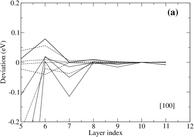
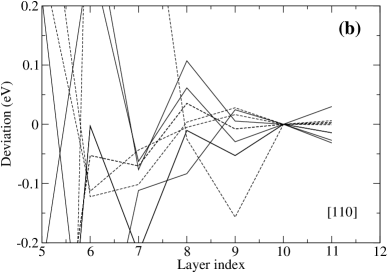
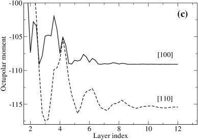
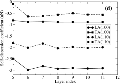
Figure 1: Convergence of various quantities with the real-space cutoff of the interatomic force constants along a given direction. (a-b): Flexocoupling coefficients along [100] and [110]; solid and dashed lines refer to longitudinal and transverse modes, respectively; the reported values are the deviations with respect to the $n=10$ point. (c): Electronic octupolar moments; the converged values are $\tilde{O}_{100}=-109.1$ a.u. and $\tilde{O}_{110}=-115.4$ a.u. (to be compared with $\tilde{O}_{100}=-108.8$ a.u. and $\tilde{O}_{110}=-115.3$ a.u., obtained in Ref. Stengel, 2014). (d) Electronic contribution to the fourth-order dispersion ($\tilde{h}^{\rm el}$).

Our calculations are performed within the local-density approximation Perdew and Wang (1992) to density-functional theory. The interactions between valence electrons and ionic cores are described by separable norm-conserving pseudopotentials in the Troullier-Martins Troullier and Martins (1991) form, generated with the fhi98PP code. Fuchs and Scheffler (1999) The reference states (the numbers in brackets indicate the core radius in bohr) of the isolated neutral atom used for the generation of the pseudopotentials are $2s$(1.4), $2p$(1.4) and $3d$(1.4) for O, $4s$(1.5), $4p$(1.5) and $4d$(2.0) for Sr and $3s$(1.3), $3p$(1.3) and $3d$(1.3) for Ti. The local angular-momentum channel is $l=2$ for Sr and O, $l=0$ for Ti. The cutoff for the wavefunction plane-wave basis is set to 300 Ry to ensure optimal accuracy in the numerical differentiations in $q$-space. The surface Brillouin zone of the SrTiO₃ primitive cell is sampled by means of a $12\times 12\times 12$ Monkhorst-Pack mesh. The long-wave expansion of the dynamical matrix is performed via the following procedure.

First, we calculate the full dynamical matrix, by means of density-functional perturbation theory Gonze (1997); Gonze and Lee (1997); Baroni et al. (2001) as implemented in ABINIT, Gonze et al. (2009) on a regularly spaced stripe of ${\bf q}$ points in reciprocal space. Compatibly with the chosen $k$-point set, we use $\Gamma$-centered stripes of 12 points spanning a line in reciprocal space, either along [100] or [110]. (The dynamical matrix at $\Gamma$ is corrected with the nonanalytical term that corresponds to the direction in ${\bf q}$-space under study, which we separately calculate by means of a standard electric field response calculation.) Second, we operate a one-dimensional Fourier transform on each matrix element, which provides us with the real-space force constants along a given direction. Such force constants decay exponentially in real space, and their moments can be therefore calculated very accurately. The convergence of any quantity with respect to the real-space cut off of the interatomic constants can be also easily monitored. These moments provide us with the desired long-wave expansion terms of the $\hat{D}$-matrices (i.e. those with the nonanalytic electrostatic terms included). Next, parallel with the analysis of the interatomic force constants we perform an analogous Fourier processing of the induced charge density, which provides us with the electronic octupolar moments, and hence with the longitudinal components of the flexoelectric tensor. Finally, by using the known relationships between short-circuit and open-circuit flexoelectric response, we appropriately combine the charge octupoles and the calculated $\hat{D}$-matrices to extract the full flexocoupling tensor components and, in turn, all the necessary quantities to study SGE and flexoelectricity in bulk SrTiO₃.

In Table 1 we report the calculated values of a few standard lattice-dynamical and dielectric properties of bulk SrTiO₃: the optical mode frequencies, their associated dynamical charges and the dielectric constant (both in the static and high-frequency limits). These quantities are shown here both for reference, and also because they are directly involved in the higher-order tensors describing the strain-gradient response of the crystal. To calculate the latter, and thereby demonstrate the formalism developed in this work, a number of additional basic ingredients are needed: the flexocoupling coefficients ($\tilde{f}$), the electronic octupolar moments, and the relevant frozen-ion SGE coefficients ($\tilde{h}$). Since these quantities are calculated as a real-space moment of some Fourier-transformed lattice-dynamical quantity, one must choose a cutoff distance beyond which the lattice sum (or the integral) is truncated. The convergence of each of the aforementioned quantities with respect to such a cutoff (expressed in number of atomic monolayers) is shown in Fig. 1. In all cases the convergence is excellent, e.g., it is of the order of 0.1 eV (i.e., well below 1%) in the flexocoupling coefficients along [110], and even (much) better in the [100] case. We shall initially report the values of the aforementioned quantities as calculated under “mixed electrical boundary conditions” (MEBC). Hong and Vanderbilt (2011) (longitudinal modes experiences an open-circuit environment, while short-circuit is naturally imposed by the periodicity of the lattice in the transverse plane), and later discuss how to recast them in a tensorial form by separating the electrostatic contribution. Consequently, the octupolar moments, $\tilde{O}_{\hat{\bf q}}$, reported in Fig. 1 are related to the longitudinal component of the frozen-ion flexoelectric tensor by $\mu_{\hat{\bf q}}=\epsilon_{\infty}\tilde{O}_{\hat{\bf q}}/6\Omega$.

IV.2 Flexocoupling coefficients in MEBC

	$[100]$		$[110]$
	L	T	L	T
A	137.13	43.46	132.02	48.59
1	$-$83.45	$-$44.53	$-$65.53	$-$27.89
2	108.45	5.84	52.15	29.92
3	$-$155.16	$-$22.87	$-$100.36	$-$89.90
S	0.00	43.70	57.33	$-$13.65

Table 2: Calculated energy flexocoupling coefficients in MEBC, corresponding to acoustic phonon modes propagating along [100] and [110]. Labels refer to the self-coupling of the acoustic mode (A), to the IR-active optical modes (1-3) and to the silent mode (S). L and T indicate longitudinal and transverse polarization, respectively. The character of the IR-active modes is consistent with the L or T label. Values are in eV units.

The central quantity that one needs when dealing with either flexoelectricity or strain-gradient elasticity is the flexocoupling tensor – for this reason we shall describe its calculation in detail. The first step, which will be outlined in this section, is the calculation of the longitudinal and transverse flexocoupling coefficients, $\tilde{f}^{\rm L,T}_{\hat{\bf q}}$, along the [100] or [110] direction in ${\bf q}$-space. These are given by the second moments (along the direction $\hat{\bf q}$) of the “bare” dynamical matrix, $\hat{D}$, i.e., with the electrostatic interactions included; this means that MEBC are naturally imposed along $\hat{\bf q}$.

One must keep in mind that the coefficients that one obtains this way are specialized to the direction $\hat{\bf q}$ and to the polarization (longitudinal or transverse) of the mode: For example, some of the $\tilde{f}$ coefficients describe the interaction between longitudinal acoustic (LA) and longitudinal optic (LO) modes ($\tilde{f}^{\rm L}$), while others couple transverse acoustic (TA) modes to transverse optic (TO) phonons ($\tilde{f}^{\rm T}$).  As TO and LO modes experience dissimilar electrical boundary conditions, they differ even at the Brillouin zone center; this implies that $\tilde{f}^{\rm L}$ coefficients cannot be mixed or compared to $\tilde{f}^{\rm T}$ coefficients, let alone treated as the components of a single tensor. (The practical procedure to extract a proper tensorial expression will be discussed shortly.)

The calculated values of the $\tilde{f}_{\hat{\bf q}}$ coefficients are reported in Table 2. In addition to the coupling to the IR-active modes, which are sensitive to the above considerations on the electrical boundary conditions, we also show the “self-coupling” of the acoustic branch (these directly relate to the relevant component of the elastic tensor), and the coupling to the “silent” (S) mode. The latter, of course, does not carry a dynamical dipole and is therefore irrelevant for flexoelectricity; still, as we shall see in the following Section, it does contribute to strain-gradient elasticity.

IV.3 Acoustic phonon dispersion

	$[100]$		$[110]$
	L	T	L	T
A	$-$2.93	$-$0.89	$-$2.03	$-$0.56
1	$-$10.76	$-$62.69	$-$6.64	$-$24.59
2	$-$2.35	$-$0.05	$-$0.54	$-$1.29
3	$-$1.61	$-$0.07	$-$0.67	$-$1.09
S	0.00	$-$1.46	$-$2.50	$-$0.14
Total	$-$17.65	$-$65.16	$-$12.39	$-$27.67

Table 3: Contributions to the dispersion of the acoustic branches in a vicinity of $\Gamma$, corresponding to the $\tilde{h}$ coefficient defined in the text. Longitudinal and transverse phonon modes propagating along [100] and [110] are considered. Labels correspond th the self-dispersion (A), IR-active optical modes (1-3) and silent mode (S). Values are in nN.

In Table 3 we report the calculated values of the $\tilde{h}$ coefficients, referring to nonlocal elastic effects in MEBC. These coefficients are further decomposed into a purely electronic (self-dispersion) term, which we shall indicate as “frozen-ion” (FI) hereafter, and a number of lattice-mediated (LM) contributions, which are associated to the relaxation of each zone-center optical modes, either IR-active or silent. (Such a decomposition is in all respects equivalent to the better-known case of linear elasticity, where the corresponding materials constants are also conveniently split into a FI and a LM contribution.) It is clear from the table that all the values are negative, i.e. both effects lead to a systematic softening of the elastic response of the crystal at short length scales. The physical mechanisms that lie behind this observation are quite dissimilar in the FI and LM cases, so I shall discuss them separately in the following, starting from the former.

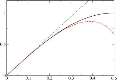
Figure 2: Dispersion relation of a linear chain (black curve) as approximated by local elasticity (green dot-dashed) and SGE (red dashed).

	First-principles		Model
	L	T	L	T
$[100]$	$-$2.93	$-$0.89	$-$4.77	$-$1.51
$[110]$	$-$2.03	$-$0.56	$-$2.30	$-$0.85
$[111]$	$-$1.87	$-$0.38	$-$1.51	$-$0.54

Table 4: Frozen-ion contribution to the SGE coefficients in MEBC (“first-principles”) compared with a rough estimation based on the 1st-neighbor lattice model described in the text (“model”). The model values were obtained by setting the $a$ parameter to the periodicity of the lattice along the phonon directions, i.e. $a_{0}$, $a_{0}/\sqrt{2}$, and $a_{0}/\sqrt{3}$ respectively along [100], [110] and [111]. Values are in nN.

To understand the origin of the self-dispersion of the acoustic branches it is instructive to consider the simple textbook model of a linear chain of atoms interacting with first-neighbor springs. The dispersion of the LA branch is trivially given by

$$\omega^{2}(q)=2\frac{k}{m}[1-\cos(qa)],$$ (97)

where $k$ is the spring constant, $m$ is the mass and $a$ is the lattice spacing. By performing a long-wave expansion to $\mathcal{O}(q^{4})$, analogously to the procedure used in the remainder of this work, one readily obtains a continuum energy functional for this system,

$$E=\frac{q^{2}}{2}\mathcal{C}+\frac{q^{4}}{2}\tilde{h},$$ (98)

where the elastic and hyperelastic constants are

$$\mathcal{C} = \,\,\,\frac{ka^{2}}{\Omega},$$ (99)

$$\tilde{h} = -\frac{ka^{4}}{12\Omega}.$$ (100)

(We have introduced the volume factor $\Omega$ by supposing that the chain of atoms is, in fact, a chain of atomic planes, consistent with the three-dimensional nature of the SrTiO₃ crystal under study.) In Fig. 2 we show a comparison of the phonon dispersion as predicted by the continuum SGE functional with the exact discrete reference. This analysis allows us to relate the two elastic coefficient as

$$\tilde{h}=-a^{2}\mathcal{C}/12.$$ (101)

This result implies that $\tilde{h}$ is primarily due to the discreteness of the lattice, and will produce measurable effects at a lengthscale that is comparable to the interatomic spacing, $a$. While SrTiO₃ is undoubtedly more complicated than this toy model, it is interesting to compare the predictions of Eq. (101) with the actual values of $\tilde{h}$ calculated from first-principles, to see if, at least qualitatively, the above ideas are correct. As one can readily appreciate from Table 4, the two sets of values display a consistent trend, and even quantitatively they lie within a factor of two in all cases, confirming that we are indeed on the right track. Such an agreement tells us that the FI contribution to strain-gradient elasticity is utterly small, and becomes relevant only at a lengthscale that is comparable to the interatomic spacing. (Similar conclusions were drawn in Ref. Maranganti and Sharma, 2007a.) Its inclusion in a continuum thermodynamic functional appears therefore of limited interest, except for guaranteeing the gauge invariance of the theory as we shall see in Section IV.5.

The LM contribution, related to the optical modes, is negative by construction, and in the transverse cases is largely dominated by the ferroelectric “soft” mode. (In the longitudinal case, the overall value of $\tilde{h}$ is more equally distributed.) That the soft mode plays a dominant role in $\tilde{h}$ is no surprise, given its very low transverse frequency (recall that the squared frequency appears at the denominator in the SGE energy) in our computational model of SrTiO₃. After the inclusion of the LM contributions, the resulting characteristic length scales (usually defined in the literature as $\xi=\sqrt{\mathcal{C}/|\tilde{h}|}$), are significantly larger compared to the previous estimation of $\xi\sim a/\sqrt{12}$, obtained at the frozen-ion level. Still, the value of $\xi$ hardly reaches 1 nm in the present first-principles model of SrTiO₃, questoning again the general relevance of the SGE (and flexoelectric) energy in continuum simulations of macroscopic phenomena. It is important, however, to emphasize a notable consequence of the theory presented so far: the above length scale diverges near a ferroelectric phase transition, i.e. when the frequency of the soft mode tends to zero. This suggests that SGE may lead to interesting physical effects whenever an optical phonon undergoes a critical behavior, and that lattice-mediated flexoelectric/SGE effects cannot a priori be neglected in such a regime.

IV.4 Macroscopic coupling tensors

	$C_{xx,xx}$	$C_{xy,xy}$	$C_{xx,yy}$
Dynamical matrix	386.2	122.4	112.6
Strain	386.2	122.4	112.6

Table 5: Calculated elastic tensor of bulk SrTiO₃. Values in the upper row were obtained by using the dynamical matrix approach described in this work. The lower row was obtained by taking finite differences of the calculated stress tensor while varying the strain around the equilibrium cubic configuration. Values are in GPa.

In this Section we shall proceed to extracting, from the results presented so far, the elastic and flexocoupling coefficients in a proper tensorial form. Regarding the elastic tensor, it can be trivially extracted from the [100] and [110] “flexocoupling” coefficients of the acoustic mode with itself. As there are four calculated values and three independent entries, the redundancy can be used as a consistency check. A second numerical test consists in comparing the values calculated this way to a more standard calculation of $\bm{\mathcal{C}}$, performed via finite differences in the strain. As one can see from the results reported in Table 5, the two procedures show essentially perfect agreement: deviations are smaller than 0.1 GPa in all cases.

Recasting the $\tilde{f}$ coefficient into a tensorial form is more delicate, and requires two preliminary steps: (i) the nonanalytic electrostatic terms need to be removed from $\hat{D}^{(2)}$, thereby obtaining $\mathcal{D}^{(2)}$; (ii) the basis of zone center-eigenmodes on which $\mathcal{D}^{(2)}$ is projected need to be calculated under isotropic short-circuit conditions, rather than MEBC. Then, just like in the elastic case, we have three independent entries and four independent values for each optical mode; this is again a stringent test of the overall consistency of the implementation. (In practice, we treat the [100] values as exact, and average the error on the [110]-related terms. The deviation is very small, of the order of 0.1–0.2 eV.) The resulting values, which are one of the main results of this work, are reported in Table 6.

Note, first of all, the strong reference dependence of the individual coefficients, which can even change sign in some cases when going from a $p$-type to a $n$-type regime. (We use “$p$-type” and “$n$-type” as shortcuts to indicate that either the valence-band edge or the conduction-band edge was chosen as the reference potential.) What this really means physically is that, if we think of SrTiO₃ as a doped semiconductor, the coupling between strain gradients and zone-center optical phonons will strongly depend on the character of the majority carriers (electrons or holes). If SrTiO₃ is in a perfectly insulating state, on the other hand, the choice of one or the other reference is completely arbitrary – what changes is just the physical meaning of the “electrostatic potential” that stems from a self-consistent solution of the electromechanical problem.

	$f_{xx,xx}$		$f_{xx,yy}$		$f_{xy,xy}$
	$n$-type	$p$-type	$n$-type	$p$-type
1	$-$51.1	$-$90.2	5.1	$-$34.0	$-$44.5
2	74.4	64.1	14.8	4.5	5.8
3	$-$181.6	$-$201.7	$-$1.4	$-$21.6	$-$22.9
S	0.0	0.0	27.3	27.3	43.7

Table 6: Calculated type-II energy flexocoupling coefficients (in eV units). For the longitudinal $(xx,xx)$ and transverse $(xx,yy)$ components, both the $n$-type and $p$-type values are shown, while the shear $(xy,xy)$ coefficient is reference-independent. The three components are often indicated in the literature as $f_{11}$, $f_{12}$ and $f_{44}$, respectively.

Not all the coupling coefficients are affected by such a reference dependence, though: The shear components $f^{j}_{xy,xy}$ (also known in the literature as $f_{44}$) are unsensitive to this arbitrariness. A closer look allows us to identify an additional linear combination of the $f$-coefficients where the ambiguity cancels out,

$$f^{\rm T}_{110}=\frac{1}{2}(f_{11}-f_{12}),$$ (102)

which is relevant for a transversally polarized (i.e., with the displacement vector oriented along [$1\bar{1}0$]) acoustic phonon propagating along [110]. Transverse phonons along any conceivable direction are described by a linear combination of the $f_{44}$ and $f^{\rm T}_{110}$ coefficients, and the reference independence is consistent with the preservation of translational periodicity along the displacement direction. Regarding the actual values, in the case of the soft mode (TO1) we obtain

$$\frac{f^{\rm TO1}_{44}}{Z^{*}_{\rm TO1}}\,\, = -1.96\,\,{\rm V}$$ (103)

$$\frac{f^{\rm TO1}_{11}-f^{\rm TO1}_{12}}{2Z^{*}_{\rm TO1}} = -1.24\,\,{\rm V}.$$ (104)

(We converted the flexocoupling coefficients to voltage units by dividing them by the mode dynamical charge for a better comparison with existing literature data.) These values seem to be in overall agreement with the existing experimental estimates ($|f_{11}-f_{12}|=$1.2–1.4 V, $|f_{44}|=$1.2–2.4 V) Kvasov and Tagantsev (2015); Yudin and Tagantsev (2013); Zubko et al. (2013); Hehlen et al. (1998).

An independent first-principles calculation of such quantities was recently reported in Ref. Kvasov and Tagantsev, 2015. Our results present significant quantitative differences, especially regarding the [110] coefficient (a value of -0.2 V was reported by Kvasov and Tagantsev). Such a discrepancy may be in part due to differences in the general computational setup (e.g. exchange and correlation functionals, pseudopotentials), but also in the specific procedure that one uses to extract the $f$-tensor from the linear-response data. We stress that a correct treatment of the electrical boundary conditions, as we have extensively discussed in the course of this work, is essential for a reliable calculation of ${\bf f}$. Interestingly, if we were to estimate the transverse components of ${\bf f}$ from the TA dispersion curves (by assuming, following Ref. Yudin and Tagantsev, 2013, that TO1 is the dominant source of curvature of the branch), we would make an error of 2% and 6%, respectively in the [100] and [110] coefficient (this can be easily inferred from the data of Table 3).

IV.5 Gauge invariance of LA phonons

	$n$-type	$p$-type	$\varphi$
A	$-$3.043	$-$2.934	$-$17.276
1	$-$257.089	$-$82.421	$-$5693.678
2	$-$5.926	$-$7.985	$-$0.828
3	$-$5.488	$-$4.449	$-$18.815
El.	253.899	80.142	5712.950
Total	$-$17.647	$-$17.647	$-$17.647

Table 7: Decomposition of the dispersion of the LA phonon along [100] into self-dispersion (A), optical modes (1-3) and electrostatic (El.) contributions. Three different assumptions for the short-circuit boundary conditions are shown: $p$-type screening (flat valence band), $n$-type screening (flat conduction band) and electrostatic screening (flat macroscopic electrostatic potential, $\varphi$). The overall result is independent of this choice, and coincides with the value ($-$17.646 nN) calculated under open-circuit conditions (see Table 3). Values are in nN.

It is useful, before closing this long Section, to perform a further consistency check of the formalism, this time by focusing on the gauge invariance. Apart from the obvious validation purposes, this exercise will provide a quantitative flavor on exactly how much the reference potential ambiguity affects the partition between SGE and Maxwell energy. As a representative example, I will focus on the dispersive behavior of the LA phonon branch along [100], whose analysis has already been presented in the first column of Table 3. In Table 3, however, the total $\tilde{h}$ coefficient was decomposed into the contributions from the LO modes and the open-circuit self-dispersion of the LA branch. Here I shall, instead, decompose the same value into contributions from TO modes, the short-circuit self-dispersion of the branch [as given by Eq. (72)], and the Maxwell energy of the flexoelectrically induced electric fields. Of course, depending on the choice of the reference potential, the individual pieces will vary but the overall sum must remain the same.

The results of this new decomposition, performed for three different choices of the reference potential are shown in Table 7. (Next to the $p$-type and $n$-type results, I also show a decomposition performed by using the bare electrostatic potential as a reference – the corresponding column is marked as $\varphi$.) The contribution of the optical phonons, as expected, is largely dominated by the soft mode (TO1). Such a contribution, which is negative definite, strongly depends on the reference, and becomes very large in the case of the bare electrostatic reference. This negative term, however, is almost exactly cancelled in all cases by an equally large and positive contribution from the Maxwell energy. The overall sum, which depends on the slight discrepancy between these two values and on the (much smaller) residual contribution from self-dispersion and other optical modes, is gauge-independent as expected, and accurately matches the value reported in Table 3.

This analysis highlights two important facts that were already anticipated earlier. First, a consistent description of strain-gradient elasticity is necessary for building a well-defined functional that incorporates flexoelectric effects. Second, insisting on choosing the electrostatic potential as a reference, as implicitly assumed in earlier ab initio works, Stengel (2014); Hong and Vanderbilt (2013) may lead to an awkward partition of the energetics between two extremely large terms, which are opposite in sign and almost exactly cancel. (This is unpalatable in practical implementations of the theory, as numerical errors might affect the two terms in a dissimilar way, and thus be artificially amplified.) This corroborates the arguments of Ref. Stengel, 2015, where the choice of the valence and conduction band edges as a reference when modeling flexoelectric phenomena was advocated for closely related reasons. Since calculations of flexoelectricity are usually performed (as in this work) in the framework of density-functional theory, adopting the valence-band edge as the energy reference appears as the most sensible choice: This is the only band energy that is, in principle, correctly described within “exact” DFT, while the physical meaning of other single-particle eigenvalues (including the conduction-band minimum) is less clear.

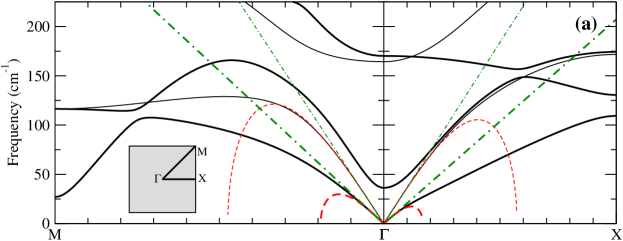
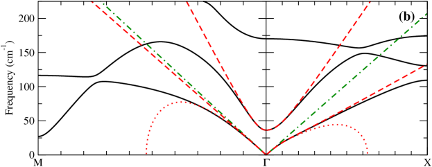
Figure 3: (a): Lattice-dynamical analysis of the continuum strain-gradient theory of Section II.1, applied to the SrTiO₃ case. Black solid curves represent the dispersion of the Fourier-interpolated ab initio phonon frequencies (thin and thick correspond, respectively, to longitudinal and transverse branches); green dot-dashed lines correspond to the linear dispersion given by classical elasticity; red dashed curves correspond to the continuum model. The inset indicates the paths in the 2D Brillouin zone that correspond to the reported phonon branches. (b): Revised continuum functional of Eq. (106), either with (dotted curves) or without (dashed curves) the “background” SGE term; only transverse modes are shown.

V Discussion

	$\Omega\mathcal{C}$	$f$	$g$
$[100]$	43.46	$-$44.53	94.26
$[110]$	48.59	$-$27.89	199.57

Table 8: Elastic constant, soft-mode flexocoupling coefficient and correlation energy (self-correlation of the soft-mode branch) associated to a transverse phonon propagating along the two directions considered in this work. Values are reported in eV.

With all the numerical data in our hands, we can now go back to the continuum thermodynamic functional proposed in Section II.1, and validate its accuracy against our reference first-principles model of SrTiO₃. Given the lattice-dynamical nature of the formalism, comparing the phonon spectrum of the continuum Lagrangian with the corresponding first-principles dispersion curves appears as an excellent way to assess the quality of the approximations that have been adopted so far. Maranganti and Sharma (2007a)

In Fig. 3 I plot the transverse and longitudinal acoustic phonon branches along [100] and [110] as predicted by the continuum model, and the whole ab initio phonon spectrum along the same directions in reciprocal space. The first observation that one can make is that the continuum model does not seem to reproduce the first-principles results very accurately: the agreement between the two breaks down only a short distance away from the zone center. For slighty larger values of $q$, the continuum curves dip downwards and plunge below zero. (In fact, the restoring force associated to larger wavevectors becomes negative, leading to an imaginary frequency and hence to an instability of the model.) This behavior is common to both longitudinal and transverse branches, although it is much more pronounced in the case of the latter. The fact that, by plugging the calculated values of the relevant coupling tensors into the strain-gradient functional of Section II.1, one obtains a pathological behavior (i.e. a thermodynamically unstable model) is no big surprise: The strain-gradient tensor ${\bf h}$ is systematically negative and enters the Hamiltonian with the highest order in the wavevector $q$, $\mathcal{O}(q^{4})$. Such a “sign” issue is well known in the literature, and seems to be a rather ubiquitous occurrence in the physics of many crystalline materials. Maranganti and Sharma (2007a) What is, on the other hand, surprising is how serious the problem is in the present SrTiO₃ case: Instabilities here occur unusually close to the zone center (compared, e.g. to the cases that were reported in Ref. Maranganti and Sharma, 2007a), which is a consequence of the strong coupling between the transverse soft-mode and acoustic branches.

Fixing this issue appears as a daunting task if one wishes to keep working with the simple strain-gradient functional of Section II.1. As we have discussed at length in the previous Section, the fourth-order dispersion of the TA branches is dominated by the interaction with the ferroelectric soft mode. As a consequence of this interaction, the SGE energy acquires a negative contribution that is inversely proportional to the square of $\omega$, the transverse soft-mode frequency. In phenomenological theories of ferroelectrics one typically assumes that this frequency follows a critical temperature behavior as

$$\omega^{2}\propto(T-T_{\rm C}),$$ (105)

where $T_{\rm C}$ is the Curie temperature; this means that the continuum model of Sec. II.1 becomes unstable at a length scale $\xi$ that diverges as $(T-T_{\rm C})^{-1/2}$. This appears difficult to fix in practical implementations; plus, the adiabatic approximation that regards optical modes as “fast” variables becomes unjustified in a proximity of $T_{\rm C}$.

An obvious way to circumvent this issue consists in modifying the functional of Sec. II.1 by promoting the soft mode to an independent degree of freedom, as it is commonly done in the ferroelectric literature. Yudin and Tagantsev (2013) For example, specializing for simplicity  to a given transverse branch along a fixed propagation direction, one can write

$$\mathcal{L}(u,\dot{u},\phi,\dot{\phi}) = \frac{\rho_{\rm mass}}{2}(\dot{\phi}^{2}-\phi^{2}\omega^{2})+\frac{\rho_{\rm mass}}{2}|\dot{u}|^{2}$$ (106)

$$-\frac{1}{2}\mathcal{C}(u^{\prime})^{2}-\frac{1}{2\Omega}g(\phi^{\prime})^{2}-\frac{1}{\Omega}f\phi^{\prime}u^{\prime}$$

$$-\frac{1}{2}h^{\rm B}(u^{\prime\prime})^{2}.$$

Here $\phi$ is the soft-mode amplitude, $g$ its correlation energy (see Section III.9), $f$ the corresponding flexocoupling coefficient, and $\mathcal{C}$ the elastic constant. The contributions to the SGE energy that are not due to the soft mode have been grouped into the “background” SGE coefficient $h^{\rm B}$; primed symbols refer to spatial derivatives along the propagation direction. It is straightforward to show that the Lagrangian of Eq. (106) reproduces, up to fourth order in $q$, the same dispersive behavior of the acoustic phonon branch as the simpler functional of Sec. II.1; thus, the two formulations provide an equally accurate description of SGE effects.

To understand why the new functional is preferrable to that of Sec. II.1 in the present SrTiO₃ case, in Fig. 3(b) we present a lattice-dynamical analysis of the dispersion curves as calculated from Eq. (106), either by including (dotted curves) or neglecting (dashed curves) the background SGE term. In the approximate ($h^{\rm B}=0$) version, which we shall discuss first, the instabilities have disappeared completely; this is a consequence of suppressing the negative $\mathcal{O}(q^{4})$ SGE contribution due to $h^{\rm B}$. One can show that the resulting functional is thermodynamically stable at any value of $\omega$ if the (now highest) $\mathcal{O}(q^{2})$ term is defined positive. This requires the following condition Axe et al. (1970); Yudin and Tagantsev (2013) to be satisfied along all directions in $q$-space,

$$\Omega\mathcal{C}g>f^{2}.$$ (107)

In Table 8 I report the values of the relevant parameters calculated in the present first-principles model of SrTiO₃ along [100] and [110]; the stability criterion, Eq. (107), is clearly satisfied in both cases. Note that although there is no explicit SGE term, the implicit contribution of the soft mode to the SGE energy, which constitutes more than 90% of the total, is correctly described via the flexocoupling term. This observation explains the remarkable accuracy of the resulting acoustic dispersion curves [dashed curves in Fig. 3(b)], especially along the [100] direction.

For several different reasons (e.g., to ensure the gauge invariance of the theory, or to study physical phenomena where strain gradients are exceptionally large Abdollahi et al. (2015), or more simply in nonferroelectric materials), one may be interested in a more accurate (i.e. beyond the soft-mode approximation) treatment of the SGE energy. If this is the case, it becomes necessary to reincorporate the background SGE effects that have been neglected in the last few paragraphs. The complete functional of Eq. (106), with the correct $h^{\rm B}$ coefficient included, yields the acoustic phonon branches that are shown as dotted curves in Fig. 3(b). While there are some improvements in the description of the dispersion in a vicinity of the zone center, most clearly along the [110] direction, the systematically negative sign of $h^{\rm B}$ brings us back to the stability issues that we have already mentioned when commenting on panel (a). [Note that the critical wavevector at which the instabilities occur is much larger than in panel (a), since part of the SGE energy has been delegated to the flexocoupling term, and is now almost unsensitive to the soft-mode frequency, $\omega$.]

The fact that most contributions to the SGE energy are negative (and hence prone to instabilities when incorporated in a continuum model) in most materials – the present results for SrTiO₃ are no exception – was observed before, Maranganti and Sharma (2007a) and several workarounds have been proposed over the years. Askes and Aifantis (2011) A popular strategy consists in replacing the unstable strain gradients with stable inertia or acceleration gradients. Askes and Aifantis (2011) This way, the dispersion of an acoustic phonon branch along a given direction can be, in principle, adjusted to match the first-principles results even without introducing an explicit SGE term. When moving to the 3D case, however, it appears unlikely that one could replace the information contained in the SGE tensor entirely via this trick. The SGE tensor, as we have shown in Sec. III.10, describes both static and dynamic effects, and while inertia gradients may be used to reproduce the latter, they cannot obviously mimick the former.

The concepts developed in this work naturally suggest two additional strategies that could be used, as an alternative to (or in combination with) the inertia gradients, to construct thermodynamically stable SGE functionals. The first, which would be ideally suited to a numerical implementation, consists in discretizing the field equations, e.g., via “quasicontinuum” methods. Dupuy et al. (2005) Such techniques have been successfully applied in the past to modeling the elastic properties of materials and nanostructures in a multiscale framework. Palla et al. (2010) Discretization naturally introduces a low-pass filter in the (spatial) frequency spectrum of the allowed solutions, and therefore looks particularly promising in the present context, where the problematic instabilities occur at exceptionally short length scales. Moreover, such an approach is consistent with the physical origin of, at least, part of the SGE energy (the frozen-ion contribution), which is precisely related to the discrete nature of the atomic lattice (see Sec. IV.3).

A second possibility involves incorporating an auxiliary vector field in the continuum model, whose physical parameters (zone-center frequency, correlation and flexocoupling coefficient) are such that: (i) the auxiliary mode is adiabatically separated from both the soft mode and the acoustic branches; (ii) its contribution to the SGE energy is equal or more negative than any calculated $h^{\rm B}$ coefficient; (iii) the stability condition Eq. (107) is satisfied. Given (i-iii), one is left then with a positive-defined ${\bf h}^{\rm B}$ tensor [the contribution from the auxiliary field, in the form of Eq. (78), must be subtracted from ${\bf h}^{\rm B}$ in order to keep the overall SGE energy unaltered]. This implies that, by introducing an additional degree of freedom in the model, and by carefully engineering its (flexo)coupling to the deformation field, one can always obtain a stable functional, and yet an exact (in relationship to the first-principles reference model) treatment of all the contributions to the SGE energy.

Exploring the details of such an approach (or of the discretization route that I have mentioned earlier) would bring me far from the main scopes of this work, and I defer it to a future publication. Still, the above discussion highlights the advantages of the strategy used in this work, i.e. of approaching continuum problems with a fundamental lattice-dynamical mindset. This way, one can not only extract realistic material-specific values of the coefficients, but also provide firm microscopic foundations to the higher-level theory, and possibly devise effective solutions to existing mathematical puzzles.

VI Conclusions

I have derived a unified formulation of flexoelectricity and strain-gradient elasticity in crystalline insulators, and discussed its implications for (incipient) ferroelectric materials. The ideas presented here are immeditely relevant to a vast range of physical phenomena involving spatial inhomogeneities in the strain or other order parameters. Such studies have traditionally been the almost exclusive realm of phenomenological approaches; this work clearly demonstrates that a fully ab initio route, via a hierachical multiscale framework, is a powerful (and very realistic) alternative.

In the present implementation, first-principles data have been used as the “exact” reference on which the continuum model is built. One should keep in mind, in this context, that ab initio approaches are not free from limitations: on one hand, there are the well-known accuracy concerns related to the approximate treatment of the exchange and correlation energy; on the other hand, direct electronic-structure methods are only practical at zero temperature, which at first sight thwarts their applicability to the accurate study of ferroelectric materials. Neither of the above two issues is, in fact, a drawback of the method described here. The present multiscale strategy is completely general, and readily applicable to an arbitrary microscopic model. (This can be either an ab initio or a classical atomistic description.) Furthermore, the long-wave approximation, combined with the quasicontinuum approach that I have mentioned in Sec. V, can be regarded as a powerful, systematic tool to construct effective Hamiltonian Zhong et al. (1994, 1995); Ponomareva et al. (2012) models. The latter have been successfully used during the past two decades as a means to exploring finite-temperature and other effects in complex ferroelectric systems. In this respect, this work may open interesting new avenues towards overcoming the stringent time- and length-scale limitations of direct ab initio approaches; exploring these opportunities will be an interesting topic for future studies.

Based on the above considerations, I expect this work to promote a closer synergy between condensed-matter theorists that are active in the field of continuum modeling with those in the first-principles community, with many exciting opportunities for future collaboration. Apart from the obvious application to flexoelectricity, the methodologies developed here are directly relevant to ferroelectrics at large, and more generally to any physical system where electrical and mechanical degrees of freedom couple in nontrivial ways.

References

- Zubko et al. (2013) P. Zubko, G. Catalan, and A. K. Tagantsev, “Flexoelectric effect in solids,” Annu. Rev. Mater. Res. 43, 387–421 (2013).
- Nguyen et al. (2013) Thanh D. Nguyen, Sheng Mao, Yao-Wen Yeh, Prashant K. Purohit, and Michael C. McAlpine, “Nanoscale flexoelectricity,” Advanced Materials 25, 946–974 (2013).
- Yudin and Tagantsev (2013) P. V. Yudin and A. K. Tagantsev, “Fundamentals of flexoelectricity in solids,” Nanotechnology 24, 432001 (2013).
- Catalan et al. (2011) G. Catalan, A. Lubk, A. H. G. Vlooswijk, E. Snoeck, C. Magen, A. Janssens, G. Rispens, G. Rijnders, D. H. A. Blank, and B. Noheda, “Flexoelectric rotation of polarization in ferroelectric thin films,” Nature Materials 10, 963–967 (2011).
- Lu et al. (2012) H. Lu, C.-W. Bark, D. Esque de los Ojos, J. Alcala, C. B. Eom, G. Catalan, and A. Gruverman, “Mechanical writing of ferroelectric polarization,” Science 336, 59–61 (2012).
- Cross (2006) L. E. Cross, “Flexoelectric effects: Charge separation in insulating solids subjected to elastic strain gradients,” J. Mater. Sci. 41, 53 (2006).
- Stengel (2013a) M. Stengel, “Flexoelectricity from density-functional perturbation theory,” Phys. Rev. B 88, 174106 (2013a).
- Stengel (2013b) M. Stengel, “Microscopic response to inhomogeneous deformations in curvilinear coordinates,” Nature Communications 4, 2693 (2013b).
- Hong and Vanderbilt (2011) J. Hong and D. Vanderbilt, “First-principles theory of frozen-ion flexoelectricity,” Phys. Rev. B 84, 180101(R) (2011).
- Hong and Vanderbilt (2013) J. Hong and D. Vanderbilt, “First-principles theory and calculation of flexoelectricity,” Phys. Rev. B 88, 174107 (2013).
- Stengel (2014) M. Stengel, “Surface control of flexoelectricity,” Phys. Rev. B 90, 201112(R) (2014).
- Abdollahi et al. (2015) Amir Abdollahi, Christian Peco, Daniel Millán, Marino Arroyo, Gustau Catalan, and Irene Arias, “Fracture toughening and toughness asymmetry induced by flexoelectricity,” Phys. Rev. B 92, 094101 (2015).
- Abdollahi et al. (2014) Amir Abdollahi, Christian Peco, Daniel Millán, Marino Arroyo, and Irene Arias, “Computational evaluation of the flexoelectric effect in dielectric solids,” Journal of Applied Physics 116, 093502 (2014).
- Stengel (2015) Massimiliano Stengel, “From flexoelectricity to absolute deformation potentials: The case of SrTiO3,” Phys. Rev. B 92, 205115 (2015).
- Bardeen and Shockley (1950) J. Bardeen and W. Shockley, “Deformation potentials and mobilities in non-polar crystals,” Phys. Rev. 80, 72–80 (1950).
- Mao and Purohit (2014) S. Mao and P. K. Purohit, “Insights into flexoelectric solids from strain-gradient elasticity,” J. Appl. Mech. 81, 081004 (2014).
- Mindlin and Eshel (1968) R. D. Mindlin and N. N. Eshel, “On first strain-gradient theories in linear elasticity,” Int. J. Solids Structures 4, 109–124 (1968).
- Askes and Aifantis (2011) Harm Askes and Elias C. Aifantis, “Gradient elasticity in statics and dynamics: An overview of formulations, length scale identification procedures, finite element implementations and new results,” International Journal of Solids and Structures 48, 1962 – 1990 (2011).
- Maranganti and Sharma (2007a) R. Maranganti and P. Sharma, “A novel atomistic approach to determine strain-gradient elasticity constants: Tabulation and comparison for various metals, semiconductors, silica, polymers and the (ir) relevance for nanotechnologies,” Journal of the Mechanics and Physics of Solids 55, 1823 – 1852 (2007a).
- Maranganti and Sharma (2007b) R. Maranganti and P. Sharma, “Length scales at which classical elasticity breaks down for various materials,” Phys. Rev. Lett. 98, 195504 (2007b).
- Axe et al. (1970) J. D. Axe, J. Harada, and G. Shirane, “Anomalous acoustic dispersion in centrosymmetric crystals with soft optic phonons,” Phys. Rev. B 1, 1227–1234 (1970).
- Tagantsev et al. (2013) A. K. Tagantsev, K. Vaideeswaran, S. B. Vakhrushev, A. V. Filimonov, R. G. Burkovsky, A. Shaganov, D. Andronikova, A. I. Rudskoy, A. Q. R. Baron, H. Uchiyama, D. Chernyshov, A. Bosak, Z. Ujma, K. Roleder, A. Majchrowski, J. H. Ko, and N. Setter, “The origin of antiferroelectricity in PbZrO3,” Nat Commun 4, 2229 (2013).
- Kvasov and Tagantsev (2015) Alexander Kvasov and Alexander K. Tagantsev, “Dynamic flexoelectric effect in perovskites from first-principles calculations,” Phys. Rev. B 92, 054104 (2015).
- Wu et al. (2005) X. Wu, D. Vanderbilt, and D. R. Hamann, “Systematic treatment of displacements, strains, and electric fields in density-functional perturbation theory,” Phys. Rev. B 72, 035105 (2005).
- Note (1) Issues of this kind are, again, well known in the piezoelectric case, where the elastic coefficients need to be defined under short-circuit electrical boundary conditions for to behave as a tensor. Wu et al. (2005).
- Van de Walle and Martin (1989) Chris G. Van de Walle and Richard M. Martin, “Absolute deformation potentials: Formulation and ab initio calculations for semiconductors,” Phys. Rev. Lett. 62, 2028–2031 (1989).
- Resta et al. (1990) R. Resta, L. Colombo, and S. Baroni, “Absolute deformation potentials in semiconductors,” Phys. Rev. B 41, 12358–12361 (1990).
- Note (2) The terms “static” and “dynamic” may refer to the physical nature of a given effect, or to the procedure that one uses to measure or calculate it. In this work I shall use the former meaning. Static properties can be studied by dynamical means and viceversa, so the two categories do not always overlap.
- Stengel et al. (2009) Massimiliano Stengel, Nicola A. Spaldin, and David Vanderbilt, “Electric displacement as the fundamental variable in electronic-structure calculations,” Nature Physics 5, 304–308 (2009).
- Born and Huang (1954) Max Born and Kun Huang, Dynamical Theory of Crystal Lattices (Oxford University Press, Oxford, 1954).
- Tagantsev (1986) A. K. Tagantsev, “Piezoelectricity and flexoelectricity in crystalline dielectrics,” Phys. Rev. B 34, 5883 (1986).
- Gonze (1995) Xavier Gonze, “Perturbation expansion of variational principles at arbitrary order,” Phys. Rev. A 52, 1086–1095 (1995).
- Martin (1972) Richard M. Martin, “Piezoelectricity,” Phys. Rev. B 5, 1607–1613 (1972).
- Pick et al. (1970) Robert M. Pick, Morrel H. Cohen, and Richard M. Martin, “Microscopic theory of force constants in the adiabatic approximation,” Phys. Rev. B 1, 910–920 (1970).
- Note (3) The matrix inversion is performed only on the optical modes subspace, leaving a null eigenvalue on the translational part.
- Cochran and Cowley (1962) W. Cochran and R.A. Cowley, “Dielectric constants and lattice vibrations,” Journal of Physics and Chemistry of Solids 23, 447 – 450 (1962).
- Resta (2010) R. Resta, “Towards a bulk theory of flexoelectricity,” Phys. Rev. Lett. 105, 127601 (2010).
- Perdew and Wang (1992) J. P. Perdew and Y. Wang, “Accurate and simple analytic representation of the electron-gas correlation energy,” Phys. Rev. B 45, 13244 (1992).
- Troullier and Martins (1991) N. Troullier and J. L. Martins, “Efficient pseudopotentials for plane-wave calculations,” Phys. Rev. B 43, 1993–2006 (1991).
- Fuchs and Scheffler (1999) M. Fuchs and M. Scheffler, “Ab initio pseudopotentials for electronic structure calculations of polyatomic systems using density-functional theory,” Computer Phys. Commun. 119, 67–98 (1999).
- Gonze (1997) Xavier Gonze, “First-principles responses of solids to atomic displacements and homogeneous electric fields: Implementation of a conjugate-gradient algorithm,” Phys. Rev. B 55, 10337–10354 (1997).
- Gonze and Lee (1997) X. Gonze and C. Lee, “Dynamical matrices, Born effective charges, dielectric permittivity tensors, and interatomic force constants from density-functional perturbation theory,” Phys. Rev. B 55, 10355 (1997).
- Baroni et al. (2001) S. Baroni, S. de Gironcoli, and A. Dal Corso, “Phonons and related crystal properties from density-functional perturbation theory,” Rev. Mod. Phys. 73, 515 (2001).
- Gonze et al. (2009) X. Gonze, B. Amadon, P.-M. Anglade, J.-M. Beuken, F. Bottin, P. Boulanger, F. Bruneval, D. Caliste, R. Caracas, M. Côté, T. Deutsch, L. Genovese, Ph. Ghosez, M. Giantomassi, S. Goedecker, D.R. Hamann, P. Hermet, F. Jollet, G. Jomard, S. Leroux, M. Mancini, S. Mazevet, M.J.T. Oliveira, G. Onida, Y. Pouillon, T. Rangel, G.-M. Rignanese, D. Sangalli, R. Shaltaf, M. Torrent, M.J. Verstraete, G. Zerah, and J.W. Zwanziger, “ABINIT: First-principles approach to material and nanosystem properties,” Computer Phys. Commun. 180, 2582 – 2615 (2009).
- Note (4) Since we are dealing with high-symmetry directions, the two subspaces of the longitudinal and transverse phonons are decoupled, and can be treated independently.
- Hehlen et al. (1998) B. Hehlen, L. Arzel, A. K. Tagantsev, E. Courtens, Y. Inaba, A. Yamanaka, and K. Inoue, “Brillouin-scattering observation of the TA-TO coupling in SrTiO3,” Phys. Rev. B 57, R13989–R13992 (1998).
- Note (5) The calculation of the full correlation matrix in a correct tensorial form presents some additional subtleties regarding the treatment of the long-range electrostatics and the gauge invariance; these would require a long digression in order to be adequately clarified.
- Dupuy et al. (2005) L. M. Dupuy, E. B. Tadmor, R. E. Miller, and R. Phillips, “Finite-temperature quasicontinuum: Molecular dynamics without all the atoms,” Phys. Rev. Lett. 95, 060202 (2005).
- Palla et al. (2010) Pier Luca Palla, Stefano Giordano, and Luciano Colombo, “Lattice model describing scale effects in nonlinear elasticity of nanoinhomogeneities,” Phys. Rev. B 81, 214113 (2010).
- Zhong et al. (1994) W. Zhong, David Vanderbilt, and K. M. Rabe, “Phase transitions in BaTi from first principles,” Phys. Rev. Lett. 73, 1861–1864 (1994).
- Zhong et al. (1995) W. Zhong, David Vanderbilt, and K. M. Rabe, “First-principles theory of ferroelectric phase transitions for perovskites: The case of BaTiO3,” Phys. Rev. B 52, 6301–6312 (1995).
- Ponomareva et al. (2012) I. Ponomareva, A. K. Tagantsev, and L. Bellaiche, “Finite-temperature flexoelectricity in ferroelectric thin films from first principles,” Phys. Rev. B 85, 104101 (2012).