Field theoretical model of multilayered Josephson junction
and dynamics of Josephson vortices
Abstract
Multi-layered Josephson junctions are modeled in the context of a field theory, and dynamics of Josephson vortices trapped inside insulators are studied. Starting from a theory consisting of complex and real scalar fields coupled to a U(1) gauge field which admit parallel domain-wall solutions, Josephson couplings are introduced weakly between the complex scalar fields. The domain walls behave as insulators separating superconductors, where one of the complex scalar fields has a gap. We construct the effective Lagrangian on the domain walls, which reduces to a coupled sine-Gordon model for well-separated walls and contains more interactions for walls at short distance. We then construct sine-Gordon solitons emerging in an effective theory in which we identify Josephson vortices carrying singly quantized magnetic fluxes. When two neighboring superconductors tend to have the same phase, the ground state does not change with the positions of domain walls (the width of superconductors). On the other hand, when two neighboring superconductors tend to have -phase differences, the ground state has a phase transition depending on the positions of domain walls; when the two walls are close to each other (one superconductor is thin), frustration occurs because of the coupling between the two superconductors besides the thin superconductor. Focusing on the case of three superconductors separated by two insulators, we find for the former case that the interaction between two Josephson vortices on different insulators changes its nature, i.e., attractive or repulsive, depending on the positions of the domain walls. In the latter case, there emerges fractional Josephson vortices when two degenerate ground states appear due to spontaneous charge-symmetry breaking, and the number of the Josephson vortices varies with the position of the domain walls. Our predictions should be verified in multilayered Josephson junctions.
1 Introduction
The Josephson effect is one of the most striking macroscopic quantum phenomena, which was theoretically predicted and experimentally confirmed in the 1960s [1, 2, 3, 4, 5]. The phenomenon is realized by a system consisting of two superconductors which are shielded by a thin insulator and are weakly interacted, called the Josephson junction. Due to the phase difference of macroscopic wavefunctions of the two superconductors, an electric current is induced even without any voltage difference between the superconductors. Now the effect became a basic ingredient in condensed-matter physics and is written in many standard textbooks (for example, see Refs.[6, 7]). Due to recent progress, the effect can be seen not only in the standard Josephson junctions but also in various weak links of superconductors consisting of new materials : graphene [8] and topological insulators [9, 10], for example. The Josephson effect is also important for engineering science. The superconducting quantum interference device (SQUID) [11] and superconducting qubits [12] are the typical examples of the application of the phenomenon.
When a magnetic field is applied parallel to a Josephson junction made of type-II superconductors, vortices (magnetic flux tubes) in the type-II superconductors are absorbed into the insulator. Such magnetic vortices trapped inside an insulator are called Josephson vortices or fluxoids [13]. The dynamics of Josephson vortices can be described by the sine-Gordon model [14, 15, 16, 17, 18]. On the other hand, studies of the vortices in various complex setups are frequently done by using the simulations of the Ginzburg-Landau (GL) model: 3D GL calculation in anisotropic mesoscopic superconductors [19], vortex-antivortex pair generation in the presence of applied electric current [20], time-dependent calculation of the vortices under an external source [21, 22, 23, 24], and so on. Josephson vortex is not a mere conceptual object in theoretical physics, but a detectable one: it is directly observed by using scanning tunneling microscopy on the surface of Si(111)-()-In [25] and in a lateral superconductor-normal-superconductor (SNS) network of superconducting Pb nanocrystals linked together by an atomically thin Pb wetting layer [26].
Some materials have structures similar to Josephson junctions. Oxide high- superconductors have a multi-layer structure of superconductors (planes of Cu2O) and insulators (other atomic layers) [27]. The coupling between the layered superconductors varies with the materials. The coupling in BSCCO (Bi2Sr2CaCu2O8+δ) [28, 29, 30, 31] is especially weak, and it is known that these materials behave like multilayered Josephson junctions, from the analysis of their current-voltage characteristics and the specific property of high-frequency electromagnetic waves: the terahertz laser is produced continuously by BSCCO due to its Josephson plasma oscillation [14, 32, 33, 34, 35], which is a collective motion of Josephson vortices and superconducting electrons and very important for applications in engineering [34, 35]. Not only the natural multilayered structure of Josephson junctions, but the artificial multilayered superconductors and insulators are also available with the development of precise processing technology: artificial construction of high- superconductors started already in the last 1980s [36], and more recently, the experiment of mesoscopic superconducting rings which make a layered structure is performed [37], for example. These developments enable us to test the theoretical prediction in various experimental setups.
In this study, we propose a simple field theoretical model describing multilayered Josephson junctions and we study the dynamics of Josephson vortices. The model for an -layered Josephson junction can be described by the model. This is a multicomponent extension of the previous study of two superconducting layers with one junction [38, 39]. We start from the (1) gauge theory with one real and complex scalar fields, similarly to the Ginzburg-Landau theory for a single superconductor. We consider the critical coupling, which is known as the Bogomol’nyi-Prasado-Sommerfield (BPS) limit in the field theory language. This assumption technically simplifies the treatment but is not essential for the dynamics of Josephson vortices. Taking the strong coupling limit of it, we obtain a massive model, where parallel domain walls are allowed behaving as insulators. Then, Josephson terms are introduced between superconductors perturbatively. We construct the low-energy effective Lagrangian of the domain walls (insulating junctions) and find that it reduces to a coupled sine-Gordon model [40, 41] in the limit of well-separated domain walls (thick superconductors) while it contains more general interaction for domain walls at short distances (thin superconductors). The effective theory allows sine-Gordon solitons carrying quantized magnetic fluxes, which we identify as Josephson vortices. Focusing on the case, where two domain walls (three superconductors and two insulators) exist, we investigate the dependence of the effective potential and the sine-Gordon solitons on the distance of the domain walls (the thickness of the middle superconductor). There are essentially the two cases depending on the Josephson coupling: When two neighboring superconductors tend to have the same phase, the ground state does not depend on the positions of domain walls (the width of the middle superconductor). When two neighboring superconductors tend to have the -phase differences, the ground state has a phase transition depending on the positions of domain walls; when the two walls are close to each other (the middle superconductor is thin), frustration occurs because of the coupling between the two superconductors besides the middle superconductor. We study dynamics of Josephson vortices both as sine-Gordon solitons in the effective theory and as full numerical configurations. In the unfrustrated case, the interaction of Josephson vortices at the two neighboring insulators changes its nature, i.e., the interaction is attractive when the two insulators are well-separated (the middle superconductor is thick), while the interaction is repulsive when they are close to each other (the middle superconductor is thin). In the frustrated case, fractional sine-Gordon solitons emerge when two degenerate ground states appear due to spontaneous charge-symmetry breaking, depending on the distance of two domain walls.
This paper is organized as follows. In Sec. 2, we construct the field theoretical model of a multilayered Josephson junction. We derive the massive model in the strong coupling limit of a (1) gauge theory coupled with real and complex scalar fields, and give the domain wall solutions. Then, the Josephson terms are introduced to the model and the effective theory of domain walls is derived. In Sec. 3, multilayered Josephson junctions in the model are explained. After a brief review of the case, where there is one domain wall, we study the case of two domain walls in . In Sec. 4, we numerically investigate the properties of Josephson vortices: the vacuum structure, the interaction between the vortices, the profiles of sine-Gordon solitons, energy densities and fluxes are studied for various setups. Section 5 is devoted to a summary and discussion. We make a comment on the possibility of realization in superconductors and discuss possible extensions such as supersymmetry and non-Abelian (color) superconductors.
2 Field theoretical model of a multi-layered Josephson junction
2.1 A model without Josephson interactions
We start with the following -invariant Abelian-Higgs system111In this paper, we study only the static problem. We consider a relativistic theory that shares common properties with non-relativistic theories usual for condensed matter systems, as far as we concentrate on static problems. See Refs. [42, 43] for corresponding non-relativistic theory.
| (1) |
where () are charged scalar fields, are Abelian gauge fields and are their field strength. In terms of the Ginzburg-Landau model, , where is the magnetic field and the electric field, are the multicomponent superconductor order parameters, the second term correspond to the kinetic term of them and their couplings to and , and the third term corresponds to their self-interaction. This Lagrangian has the global symmetry which rotates the complex scalar fields . The scalar potential is minimized when the scalar fields have vacuum expectation values (VEV; i.e., condensations) such that
| (2) |
As well as the gauge symmetry, the global symmetry is spontaneously broken to by the nonzero VEVs of the charged scalar fields . Therefore, the low-energy degrees of freedom are the Nambu-Goldstone (NG) modes parametrizing the complex projective space
| (3) |
In other words, this system is described by the nonlinear sigma model when the energy scale is much smaller than the masses and of the massive photon and massive scaler field, respectively. [ and are the penetration depth and coherence length, respectively.]
Let us deform the model so that only one of can have a nonzero VEV by introducing a neutral real scalar field and mass parameters . We then add the following terms into the original Lagrangian:
| (4) |
The potential in the total Lagrangian is minimized when the scalar fields satisfy
| (5) |
There are degenerated ground states labeled by , each of which is characterized by the following VEVs of the scalar fields
| (8) |
In the following, we consider domain walls interpolating these discrete generate vacua (see Fig. 1). It will turn out that they have the role of insulating junctions in the following discussions.
To discuss the property of the domain walls, it is convenient to consider a limit in which the system is described by a simplified model. Since the mass of the fluctuation of is , its dynamics is decoupled in the low-energy limit . The parameters explicitly break the symmetry to the Cartan subgroup and hence give masses to the NG modes. Therefore, in the low-energy regime where , the system is described by the nonlinear sigma model with mass terms. The corresponding action can be obtained by taking the limit , and then eliminating the heavy degrees of freedom and by solving their equations of motion:
| (9) |
where the charged scalar fields must satisfy the constraint . To write down the effective Lagrangian, it is convenient to introduce the inhomogeneous coordinates of defined by
| (10) |
where we have used the gauge transformation to fix the overall phase so that . Then, we can rewrite the original Lagrangian in the limit into the following form
| (11) |
where and the Fubini-Study metric of is given by
| (12) |
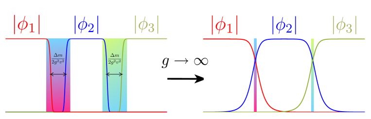
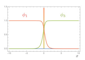
Figure 1 shows a domain-wall configuration for before and after taking the limit. The regions with different condensations are separated by the domain walls, whereas there is no condensation inside the walls. Thus, the domain walls can be regarded as the insulating junctions separating each superconductor in terms of Josephson junctions in condensed matter physics. The width of the wall can be estimated as (for ) and hence the sigma model limit corresponds to a thin-wall limit.
2.2 Domain wall solutions: inserting insulators
Next, let us consider domain-wall solutions in the massive nonlinear sigma model in Eq. (11) [44]. Suppose that the fields depend only on one of the spatial coordinates . Then the energy of the system can be rewritten as
| (13) |
Since the total derivative term is a constant for a fixed boundary condition, the energy is minimized when satisfy
| (14) |
The domain-wall solution is given by
| (15) |
where and are arbitrary parameters. Going back to the original description in terms of , we can see that there are domain walls interpolating the regions with different condensations (see Fig. 1).
The parameters are related to the domain-wall positions, which can be read from the energy density of the configuration
| (16) |
This is small in the regions where only one of the terms in the logarithm is large. Therefore, the domain walls are localized where any two terms in the logarithm are of the same order of magnitude. Suppose that the masses are ordered as . Then we can determine their positions as [45]
| (17) |
where and .
The parameters are related to the phases of . In the regions where only one of is nonzero, can be eliminated by gauge transformations. On the th domain wall (), there is an overlap of and , so that the relative phase cannot be eliminated. Since those relative phases are rotated by the global symmetry, can be viewed as the NG modes associated with the symmetry broken by the domain walls.
Now let us derive the low-energy effective model describing the dynamics of the degrees of freedom living on the domain walls. To write down the effective Lagrangian, it is convenient to introduce the complex moduli parameters defined by
| (18) |
In the low-energy regime, we can assume that weakly depends on time and the coordinates on the domain walls. Then substituting the solution into the original Lagrangian (11), we obtain the effective action of the form
| (19) |
where are the spatial directions perpendicular to . The constants are the tensions (energy per unit area) of the domain walls and the moduli space metric is given by
| (20) |
The effective theory in the nonrelativistic case can be found in Ref. [42] for the model.
In the following, we consider modifications to the domain-wall effective Lagrangian in the presence of Josephson terms and then study the solitons, assuming that the domain walls are static and the Josephson terms are weak.
2.3 Introduction of Josephson interactions
In this subsection, we construct the effective Lagrangian of the domain walls in the presence of Josephson terms. Let us consider the following deformation term which breaks the global symmetry:
| (21) |
where is a Hermitian matrix whose diagonal elements are all equal to zero. This term induces a potential term in the domain-wall effective action. For small , the leading order effective potential can be obtained by simply substituting the domain-wall solution Eq. (15) into and integrating over :
| (22) |
where .
The domain-wall effective action with this potential can be regarded as multilayered Josephson junctions; when the expectation values of are localized in different domains, they can be viewed as bulk superconductors, and the domain walls in between correspond to thin insulators as depicted in Fig. 1. Since the essence of the model as the multilayered Josephson junctions is summarized in the case, we focus on concrete calculations in the case after reviewing the case of .
3 Multi-layered Josephson junctions
3.1 A single Josephson junction of two superconductors and a Josephson vortex in it: a review
For with , the domain wall solution in the massive model takes the form [46]
| (23) |
where and are arbitrary parameters corresponding to the position and phase of the domain wall. In the case of , we can always redefine the phase of so that the coupling constant in the Josephson term is real and positive. For small , the effective action on the domain wall is given by the sine-Gordon model [38]
| (24) |
The potential term has the minimum at .
As is well known, the sine-Gordon model has kink solutions which are characterized by a nontrivial winding of . The equation describing static kink solutions can be found by setting , assuming that depends only on a spatial coordinate and rewriting the energy density as
| (25) |
This is minimized when satisfies
| (26) |
and the solution is given by
| (27) |
where is an arbitrary parameter corresponding to the kink position. The total derivative term in Eq. (25) gives the mass of the kink:
| (28) |
This object has a quantized magnetic flux: using Eq. (9), we find that
| (29) |
This is precisely a Josephson vortex, which is a magnetic vortex trapped inside an insulator [13].
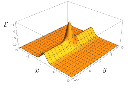
Figure 2 shows a numerical solution of the original model without taking the sigma model limit. The domain wall is localized along the line , on which the kink is localized at .
In the case of , the phase of can always be absorbed into a constant shift of , i.e., a redefinition of the phases of . As we will see, in the case of , one of cannot be absorbed by shift of and the property of the kinks depends on its value.
3.2 Three-layered Josephson junctions
Next, let us consider the case. In the following, we set
| (30) |
for simplicity. By the redefinition , the phases of are shifted as
| (31) |
This implies that the phase of does not change, and hence there is a physical phase parameter which cannot be eliminated by the redefinition. By appropriately choosing the phases of , we can always set
| (32) |
When or , the Hermitian matrix becomes a real symmetric matrix, so that the Josephson term preserves the charge conjugation symmetry
| (33) |
In the following, we focus on these two special cases: are all positive () or negative ().
To write down the effective action of the domain walls, it is convenient to use the phase differences
| (34) |
Note that and we have set in Eq. (10) by using the gauge transformation.
In this setup, the domain-wall solution is given by
| (35) |
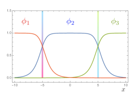
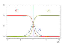
where and are the positions of two domain walls (see Fig. 3).
 |
 |
 |
| (a) | (b) | (c) |
Here we consider the large-tension limit in which dynamics of and are negligible 222In addition, we need the condition , to satisfy the potential from the 2nd-order perturbation induced by the interaction of 1st and 2nd layer and that of 2nd and 3rd layer, which is of order , is negligible compared to the 1st-order interaction of 1st and 3rd layer, which is of order .. The phase part of the effective Lagrangian takes the form
| (36) | ||||
where and are given by
| (37) |
The function can be viewed as the relative distance between the walls (see Appendix D of [47] for more details). Since for large , the parameter can be viewed as the asymptotic relative distance as we have seen in the previous section. For negative , the function gives the precise definition of the relative distance (see Fig. 5).
The effective potential is given by
| (38) | ||||
Since the potential depends only on , we set in the following. By the redefinition of the coupling constants , the parameter becomes an overall constant of the effective action, so that we can set in the classical discussion.
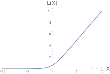
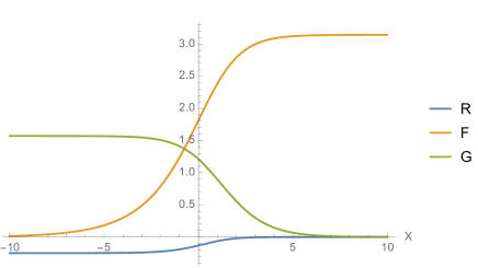
Figure 5 shows the plot of the functions , and . Since and are small for large , the interaction between and ( and ) is negligible for well separated walls and hence the effective action reduces to that for two independent walls. On the other hand, the interaction terms become relevant when two walls approach each other. Note that, for in the limit , the effective Lagrangian is independent of and reduces to that of a single wall depending only on .
The structure of minima of depends on the signs of . In the following, we restrict ourselves to the case where . Then, there are two cases: and . We study the potential, the vacuum structure, and the properties of sine-Gordon solitons in each case.
To find solutions of equations of motion, we numerically solve the gradient flow equations
| (39) |
where is a fictitious time and is the effective action corresponding to Eq. (36). Starting with an initial condition with a nontrivial topological number, we can find a minimum of by taking the limit. Although we cannot take the limit if there is no stable minimum in the topological sector, quasistable configurations can be obtained by solving the gradient flow equation for a sufficiently long time interval.
4 Interaction between Josephson vortices
4.1 : the same phases
Here, we study the properties of sine-Gordon solitons in the effective theory with .
4.1.1 Ground state
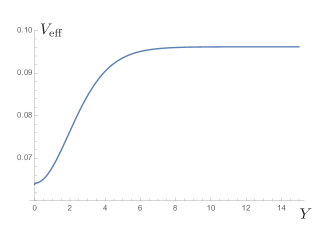
In this case, the minimum of is always located at (mod ) irrespective of the distance between two walls.
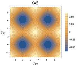
Figure 6 shows effective potentials at and . Although the shapes of the potential are different, the minima of the potential can be seen at (mod ) in both cases.
4.1.2 : the vortex-vortex interaction
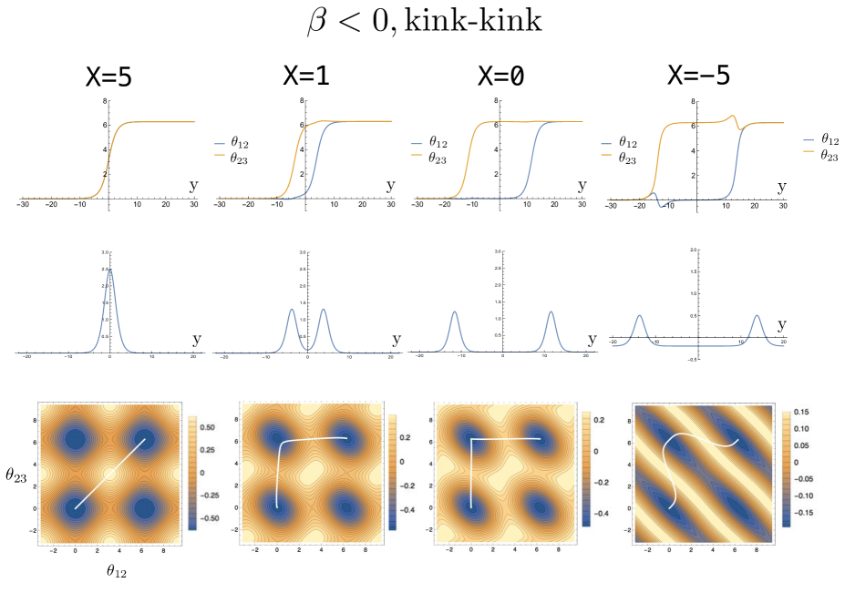
Figure 7 shows the sine-Gordon solitons on domain walls with and various values of . We call these solitons “ kinks”, since each phase degree of freedom has a single winding number. As shown in the figure with , the two solitons tend to merge with each other for large ; i.e., there is an attractive force between them. The leading order interaction potential for large can be obtained by substituting the two sine-Gordon kink configurations,
| (40) |
into the domain-wall effective action, since this is a solution of the equation of motion in the large- limit. The interaction between and gives the leading order term
| (41) |
Since the phases and tend to align with each other, the interaction potential is minimized when and hence there is a attractive force for large (see the left panel of Fig. 8). Ignoring -independent terms, we find that
| (42) |
On the other hand, as becomes smaller, the two kinks start to depart from each other, as can be seen in the figure with and in Fig. 7. Thus, the interaction becomes repulsive for small . In the limit, this configuration is reduced to two sine-Gordon kinks in the single-wall effective action and their interaction is known to be repulsive. Note that configurations in Fig. 7 are quasistable, implying that the distance between the kinks becomes larger as the fictitious time goes by.
4.1.3 : the vortex-anti-vortex interaction
Figure 9 shows configurations of “-kink.” In this case, the asymptotic interaction potential between the kink and antikink takes the form
| (43) |
As can be seen from Fig. 8, the asymptotic interaction for large is repulsive for large and attractive for small . Actually, for , we have checked by numerical calculations that the interaction is repulsive for large and attractive for small . The interaction changes its sign around . These results are consistent with the expectations from the potential of Eq. (43).
As two domain walls approach each other, the repulsive force at large changes to an attractive one suddenly at , implying the attraction for all range of .
At , the potential is almost constant along and there is almost no localized energy. This means that the kink on a domain wall and antikink on the other domain wall annihilate each other.
4.2 : -phases and frustration
Next, we study the properties of sine-Gordon solitons for .
4.2.1 Ground state
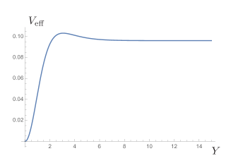
In this case, the ground state structure changes depending on the distance of two walls.
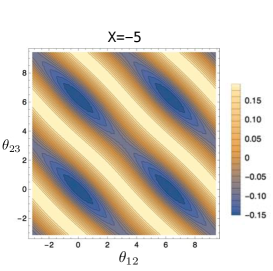
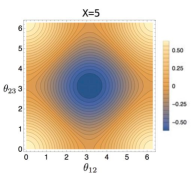
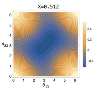
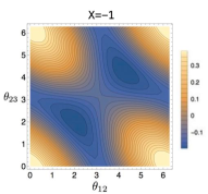
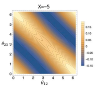
Figure 11 shows the effective potential at . For large , the term is dominant in and its minimum is located at (mod ). On the other hand, as becomes smaller, the term , which has minima at (mod ), becomes relevant. The two conditions, and , cannot be satisfied simultaneously and hence there is a frustration for small .
We can easily see that is a stationary point of :
| (44) |
At this point, the charge conjugation symmetry is preserved. The Hessian (the determinant of the second derivatives) of around the stationary point is given by
| (45) |
Here is a monotonically decreasing function such that and and hence there is a critical value at which changes its sign. Since for large , the point is a stable minimum when two domain walls are well separated. On the other hand, for , the minimum splits into a pair of points which are exchanged by the charge conjugation. Thus, is the critical value at which the charge conjugation symmetry is spontaneously broken. For , the critical value is
| (46) |
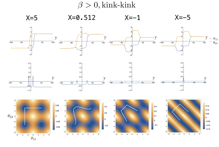
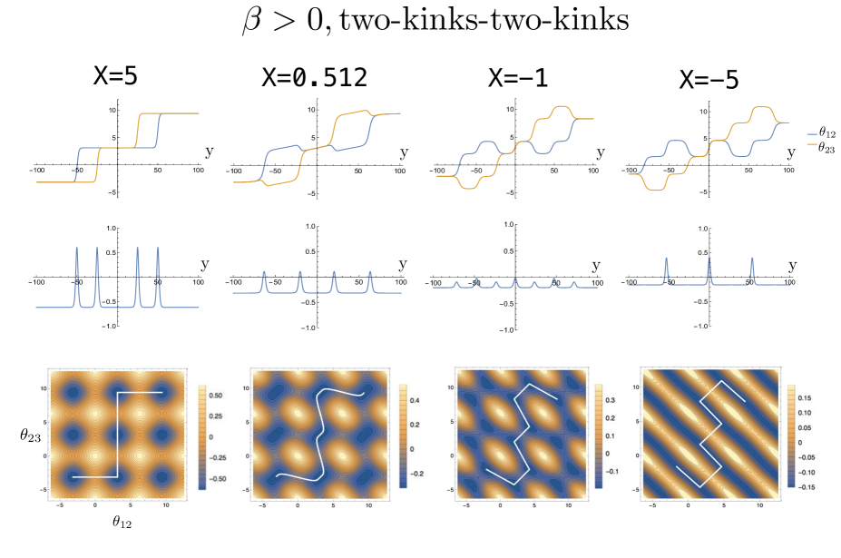
4.2.2 : the vortex-vortex interaction
Figure 11 shows the configurations of solitons with . At , the two solitons weakly repel each other. The asymptotic interaction potential between them takes the same form as Eq. (42) with the opposite sign. At , the minimum of the potential splits into the pair of vacua and there emerges another kink connecting them. For small , solitons connect the two vacua , as shown in the right figures in Fig. 11. Although it appears that there are three kinks (see case in Fig.11), two of them have very small energy since becomes unphysical as . Thus, only one kink is left in the small- limit.
Distribution of magnetic fluxes in the Josephson junction gives the important information of Josephson vortices, and is one of the main subjects of studies of the Josephson effect [19, 20, 21, 22, 23, 24]. For the vortex-vortex interaction in the frustrated case, a remarkable consequence of the change of vacuum structure can be seen in the magnetic flux:
| (47) |
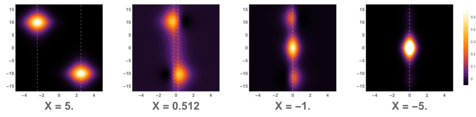
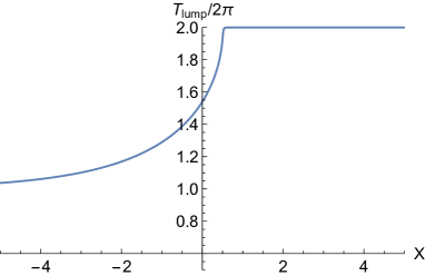
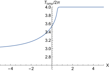
Figures. 12 and 13 show the magnetic flux distribution and the total flux of the solitons in Fig. 11, respectively. For , there are two units of magnetic flux. On the other hand, for , the flux begins to decrease due to the emergence of two vacua: each soliton becomes a “fractional soliton,” which connects a pair of inequivalent vacua. The configuration in the small- limit has one unit of magnetic flux since the solitons connect and .
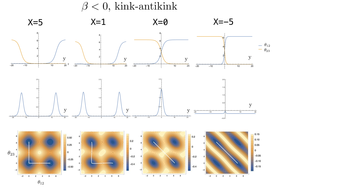
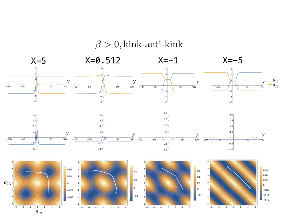
4.2.3 : the vortex-anti-vortex interaction
Figure 14 shows the configurations of solitons. At , both the kink and antikink are located around . The asymptotic interaction potential between them takes the same form as Eq. (43) with the opposite sign. Since the minimum is located at , the kink and anti-kink keep a small distance between them. As becomes smaller, the solitons change their form and their masses gradually decrease due to the change of the potential. Finally, no localized energy is left at since only the relative phase has kinks and it becomes unphysical in the small- limit. Note that flux is always zero in this case.
4.2.4 : the vortex-vortex interaction
5 Summary and discussions
We have proposed the model as a model to describe an -layered Josephson junction. To illustrate use, we have studied dynamics of Josephson vortices by studying the sine-Gordon solitons on multiple domain walls. For , we have investigated the two cases in which the charge conjugation symmetry is preserved. When the coupling constants are all positive, the vacuum structure on the domain walls is independent of their relative distance, whereas the structure changes at a critical distance when are all negative.
In the former case, the interaction between Josephson vortices on different domain walls changes with the distance between two domain walls. For solitons (kink-kink configuration), the interaction is attractive at large and repulsive at small . In the case of the solitons (kink-antikink configuration), the interaction is repulsive at large and attractive at small for , while it becomes attractive for all ranges of for .
In the latter case, the properties of the Josephson vortices change depending on the distance between the domain walls. There is a critical value at which the charge conjugation symmetry is spontaneously broken on the domain walls. For , the total magnetic flux is constant, whereas for , the flux gradually decreases as becomes smaller and hence there emerge fractional sine-Gordon solitons.
Here we comment on the related studies with our frustrated multiband superconductors.
In Ref. [48], the system of two-band superconductors is discussed and the collective excitation with respect to the fluctuations of the relative phase of two condensates is found, which is a kind of Josephson effect. The excitation, the Leggett mode, is actually observed in experiments on Mg-B2 [49, 50]. Theoretically, the excitation with fractional flux quanta is discussed in several works [51, 52, 53, 54, 37, 55]. In the stream of the studies, the system with three or more condensations and frustration between them has recently been given attention. In Ref. [56], the system was studied in which three superconductor bands are connected via repulsive pair-scattering terms, where a time-reversal-symmetry breaking (TRSB) state emerges. The Ginzburg-Landau theory is derived from the multiband BCS Hamiltonian in the general case in Ref. [57]. In Refs. [58, 59, 59], Josephson junctions between chiral and regular superconductors were considered: the asymmetric critical currents, subharmonic Shapiro steps, symmetric Fraunhofer patterns [58], and the fractional flux and its plateau in magnetization curve [59, 60] are studied by using Bogoliubov–de Gennes and the time-dependent Ginzburg-Landau equation. Also, in Ref.[61], the phase diagram of the system was investigated in the - plane.
Here we address several discussions.
In this system, the plasma oscillations occur. Due to the change of vacuum structure, the properties of plasma oscillations, such as dispersion relations, vary with the positions of domain walls. This is a peculiar property for the multilayered Josephson junctions. The analysis will be reported elsewhere.
It is curious as to whether there is a real system described by the model. The system constructed of three superconductors and two thin insulators in between may be described by the model. If the strength of the couplings can be changed and the distance between the two insulators can be controlled, we can see the change of the interaction between the solitons, and the emergence of the fractional sine-Gordon solitons.
We consider another possible experimental setup than the normal layers, which is pictorially shown in Fig. 17. Superconductors 1 (sc1), 2 (sc2), and 3 (sc3) are divided by thin insulators (black lines). The sc2 has the form of an acute-angled triangle. In this setup, the pairwise coupling of sc1 and sc3 is dominant in the upper part. On the other hand, the couplings between sc1 and sc2, and sc2 and sc3, become dominant in the lower part. There occurs frustration around the node of the insulators, and we could see the fractional vortices on the thin insulators. The distance of sc1 and sc3 is spatially and moderately dependent on the position of the vertical direction of Fig. 17. We may realize the situation that we want somewhere in the vertical direction. If we can make the setup artificially or accidentally in experiment, and make many vortices on the insulators especially around the node, we may observe a fractional vortex by manipulating a vortex using the scanning tunneling microscope and by placing it on the node.
An appropriate setup might be also realized in Bose-Einstein condensates (BECs) of ultracold-atomic gases. Mixture of two or more condensates of hyperfine states of a single atom provide multicomponent BECs. When they are repulsive a phase separation occurs to form domain walls. We can introduce Rabi oscillations to provide Josephson couplings. In this case, in principle, one might consider both unfrustrated [62] and frustrated [63] cases.
In this paper, we have regarded the domain walls as infinitely heavy and analyze the sine-Gordon kinks by fixing the positions of the domain walls. Without such an assumption, the domain walls can move giving flexible Josephson junctions. The analysis of full dynamics of the system, i.e., the time and space dependence of domain walls and the sine-Gordon solitons on the walls, should be interesting, as in Ref. [64] for the two component case.
The model admits a junction of domain walls which meet at a junction point [65], if we introduce complex masses for . More generally, the model admits a network of junctions. The effective action of such a network was obtained in Ref. [66]. This can be applied to a -shaped insulator of Josephson junctions of three superconductors if we introduce Josephson interactions. Introducing Josephson interaction to this case is an interesting problem.
In this paper, we applied magnetic field in parallel with insulators so that vortices are absorbed along the insulators to become Josephson vortices. If we apply magnetic field orthogonal to the insulators, magnetic vortices end up with the insulators, where two magnetic vortices in neighboring superconductors are connected by pancake vortices [27]. The same configurations without the Josephson interaction is a D-brane soliton [67, 68]. In particular, the most general analytic solutions in the model (relevant for layered Josephson junctions) was obtained in Ref. [68]. The effective action and dynamics of such a system were studied in Ref. [47] without the Josephson interaction. Introducing the Josephson interactions in this system should be interesting for the study of pancake vortices in field theory.
If we consider a quadratic Josephson term instead of the linear Josephson term considered in this paper, the system can be made supersymmetric by appropriately adding fermions as was shown for the case [69]. In this case, the minimum Josephson vortices carry half fluxes, and the total configurations are 1/4 BPS preserving a quarter of supersymmetry. The situation should be the same for the case of the multilayered Josephson junction studied in this paper.
Domain-wall solutions in non-Abelian gauge theory were constructed in Refs. [45, 70]. A non-Abelian generalization of Josephson junctions was proposed in Refs. [71] in which a junction of two non-Abelian (color) superconductors was discussed. The low-energy effective action of the non-Abelian domain wall (insulator) can be described by a chiral Lagrangian [72] with a pion mass term (non-Abelian sine-Gordon model) [73], admitting a non-Abelian sine-Gordon soliton [73, 74] which corresponds to a non-Abelian Josephson vortex [71]. A multilayered non-Abelian Josephson junction is one of the possible future directions.
Acknowledgments
We would like to thank Zhao Huang for useful comments and discussions and Naoki Yamamoto for a discussion at the early stage of this work. This work is supported by the Ministry of Education, Culture, Sports, Science, and Technology (MEXT) Supported Program for the Strategic Research Foundation at Private Universities “Topological Science” (Grant No. S1511006). The work of M.N. is also supported in part by a Grant-in-Aid for Scientific Research on Innovative Areas “Topological Materials Science” (KAKENHI Grant No. 15H05855) and “Nuclear Matter in Neutron Stars Investigated by Experiments and Astronomical Observations” (KAKENHI Grant No. 15H00841) from the MEXT of Japan and by a Japan Society for the Promotion of Science (JSPS) Grant-in-Aid for Scientific Research (KAKENHI Grant No. 16H03984). H.I. was supported by the RSF grant 15-12-20008.
m

References
- [1] B. D. Josephson, “The relativistic shift in the Mössbauer effect and coupled superconductors,” Dissertation for the annual election of fellows, Trinity College, Cambridge (1962); “Possible new effects in superconductive tunneling,” Phys. Lett. 1, 251-253 (1962); “Coupled superconductors,” Rev. Mod. Phys. 36, 216-220 (1964); “Supercurrents through barriers,” Adv. Phys. 14, 419-451 (1965); Superconductivity (R.D.Parks, Ed.) Vol.1, Marcel Dekker, New York, Chap.9, 423-448 (1969); “The discovery of tunneling supercurrents,” Rev. Mod. Phys. 46, 251-254 (1974).
- [2] P. W. Anderson and J. M. Rowell, “Probable observation of the Josephson superconducting tunneling effect,” Phys. Rev. Lett 10, 230-232 (1963).
- [3] S. Shapiro, “Josephson currents in superconducting tunneling: The effect of microwaves and other observations,” Phys. Rev. Lett.11, 80-82 (1963).
- [4] J. M. Rowell, “Magnetic Field Dependence of the Josephson Tunnel Current,” Phys. Rev. Lett. 11, 200-202 (1963).
- [5] P.G. De Gennes, “Boundary effects in superconductors,” Rev. Mod. Phys. 36, 225-237 (1964).
- [6] M. Tinkham, “Introduction to Superconductivity” (McGraw Hill, 1996).
- [7] A. Barone and G. Parteno, “Physics and Applications of the Josephson Effect” (Wiley, 1982).
- [8] H.B. Heersche, P. Jarrillo-Herrero, O.O. Oostinga, L.M.K. Vandersypen and A.F. Morpurgo, “Bipolarsupercurrent in graphene,” Nature 446, 56-59 (2007).
- [9] M. Veldhorst et al., “Josephson supercurrent through a topological insulator surface state,” Nature Mater. 11, 417-421 (2012).
- [10] J.R. Williams, A.J. Bestwick, P. Gallagher, S.S. Hong, Y. Cui, A.S. Bleich, J.G. Analytis, I.R. Fisher, D. Goldhaber-Gordon, “Unconventional Josephson effect in hybrid superconductor-topological insulator devices,” Phys. Rev. Lett.109, 056803 (2012).
- [11] R. C. Jaklevic, J. Lambe, A. H. Silver and J. E. Mercereau, “Quantum interference effects in Josephson tunneling,” Phys. Rev. Lett. 12, 159-160 (1964); “Quantum Interference from a Static Vector Potential in a Field-Free Region,” Phys. Rev. Lett. 12, 274-275 (1964); “Macroscopic Quantum Interference in Superconductors,” Phys. Rev. 140, A1628-1637 (1965).
- [12] M. Devoret and R. Schoelkopf, “Superconducting circuits for quantum information: An outlook,” Science 339, 1169-1174 (2013).
- [13] A. V. Ustinov, “Solitons in Josephson junctions,” Physica D 123, 315-329 (1998).
- [14] P.W. Anderson, “Special effects in superconductivity” in “Lectures on the Manybody Problem,” Ravello, 1963 (E.R. Caianiello, Ed.), Vol.2, Academic, 113-135 (1964).
- [15] A. Barone, “Flux flow effect in Josephson tunnel junctions,” J. Appl. Phys. 42, 2747 (1971).
- [16] J.Rubinstein, “Sine-Gordon equation,” J. Math. Phys. 11, 258-266 (1970).
- [17] A.C. Scott, F.Y.F. Chu and D.W. McLaughlin, “The soliton: A new concept in applied science,” Proc. IEEE 61, 1443-1483 (1973).
- [18] G.B. Witham, “Linear and Nonlinear Waves” (Wiley-Interscience, New York, 1975).
- [19] C-Y Liu, G.R.Berdiyorov and M.V.Milosevic, “Vortex states in layered mesoscopic superconductors,” Phys.Rev.B83, 104524(2011).
- [20] G.R.Berdiyorov, M.V.Milosevic, S.Savel’ev, F.Kusmartsev and F.M.Peeters, “Parametric amplification of vortex-antivortex pair generation in a Josephson junction,” Phys.Rev.B90, 134505 (2014).
- [21] G.R.Berdiyorov, S.E.Savel’ev, M.V.Milosevic, F.V.Kusmartsev and F.M.Peeters, “Synchronized dynamics of Josephson vortices in artificial stacks of SNS Josephson junctions under both dc and ac bias currents,” Phys.Rev.B87, 184510 (2013).
- [22] G.R.Berdiyorov, S.E.Savel’ev, F.V.Kusmartsev and F.M.Peeters, “In-phase motion of Josephson vortices in stacked SNS Josephson junctions: effect of ordered pinning,” Supercond. Sci. Technol. 26 (2013) 125010.
- [23] G.R.Berdiyorov, K.Harrabi, J.P.Maneval and F.M.Peeters, “Effect of pinning on the response of superconducting strips to an external current,” Supercond. Sci. Technol. 28 (2015) 025004.
- [24] G.R.Berdiyorov, M.V.Milosevic, L.Covaci, and F.M.Peeters, “Fectification by an Imprinted Phase in a Josephson Junction,” Phys.Rev.Lett.107, 177008 (2011).
- [25] S. Yoshizawa, H. Kim, T. Kawakami, Y. Nagai, T. Nakayama, X. Hu, Y. Hasegawa and T. Uchihashi, “Imaging Josephson Vortices on the Surface Superconductor Si(1,1,1)-()-In using a Scanning Tunneling Microscompe,” Phys. Rev. Lett. 113, 247004 (2014).
- [26] D. Roditchev et al., “Direct observation of Josephson vortex cores,” Nature Physics 11, 332-337 (2015).
- [27] G. Blatter, M. V. Feigel’man, V. B. Geshkenbein, A. I. Larkin, and V. M. Vinokur, “Vortices in high-temperature superconductors,” Rev. Mod. Phys. 66, 1125-1388 (1994)
- [28] H. Maeda, Y. Tanaka, M. Fukutomi and T. Asano, “A New High- Oxide Superconductor without a Rare Earth Element,” Japan J. of Appl. Phys. 27, L209-L210 (1988).
- [29] M. A. Subramanian et al., “A New High-Temperature Superconductor: Bi2Sr3-xCaxCu2O8+y,” Science 239, 1015-1017 (1988).
- [30] S. A. Sunshine et al., “Structure and physical properties of single crystals of the 84-K superconductor Bi2.2Sr2Ca0.8Cu2O8+δ,” Phys. Rev. B 38(R), 893-896 (1988).
- [31] J. L. Tallon et al., “High- superconducting phases in the series Bi2.1(Ca,Sr)n+1CunO2n+4+δ,” Nature 333, 153-156 (1988).
- [32] B. D. Josephson, Quantum Fluids (D.F.Brewer, Ed.). North Holland, Amsterdam, 174-179 (1966).
- [33] A. J. Dahm, A. Denenstein, T. F. Finnegan, D. N. Langenberg and D. J. Scalapino, “Study of the Josephson Plasma Resonance,” Phys. Rev. Lett. 20, 859-863 (1968); Errata: Phys. Rev. Lett. 20, 1020 (1968).
- [34] L. Ozyuzer et al., “Emission of coherent THz radiation from superconductors,” Science 318, 1291-1293 (2007).
- [35] U. Ulrich Welp, K. Kadowaki and R. Kleiner, “Superconducting emissions of THz radiation,” Nature Photon. 7, 702-710 (2013).
- [36] J.-M. Triscone, M.G. Karkut, L. Antognazza, O. Brunner and Ø.Fischer, “Y-Ba-Cu-O/Dy-Ba-Cu-O Superlattices: A First Step towards the Artificial Construction of High- Superconductors,” Phys. Rev. Lett.63, 1016-1019 (1989).
- [37] H. Bluhm, N.C. Koshnick, M.E. Huber and K.A. Moler, “Magnetic Response of Mesoscopic Superconducting Rings with Two Order Parameters,” Phys. Rev. Lett.97, 237002 (2006).
- [38] M. Nitta, “Josephson vortices and the Atiyah-Manton construction,” Phys. Rev. D 86, 125004 (2012) [arXiv:1207.6958 [hep-th]].
- [39] M. Kobayashi and M. Nitta, “Sine-Gordon kinks on a domain wall ring,” Phys. Rev. D 87, no. 8, 085003 (2013) [arXiv:1302.0989 [hep-th]].
- [40] S. Sakai, P. Bodin and N. F. Pedersen, “Fluxons in thin-film superconductor-insulator superlattices,” Jour. Appl. Phys.73, 2411 (1993).
- [41] N. F. Pedersen and S. Sakai, “Josephson plasma resonance in superconducting multilayers,” Phys. Rev. B58, 2820 (1998).
- [42] M. Kobayashi and M. Nitta, “Nonrelativistic Nambu-Goldstone Modes Associated with Spontaneously Broken Space-Time and Internal Symmetries,” Phys. Rev. Lett. 113, no. 12, 120403 (2014) [arXiv:1402.6826 [hep-th]].
- [43] M. Kobayashi and M. Nitta, “Nonrelativistic Nambu-Goldstone modes propagating along a Skyrmion line,” Phys. Rev. D 90, no. 2, 025010 (2014) [arXiv:1403.4031 [hep-th]].
- [44] J. P. Gauntlett, D. Tong and P. K. Townsend, “Multidomain walls in massive supersymmetric sigma models,” Phys. Rev. D 64, 025010 (2001) [hep-th/0012178]; D. Tong, “The Moduli space of BPS domain walls,” Phys. Rev. D 66, 025013 (2002) [hep-th/0202012].
- [45] Y. Isozumi, M. Nitta, K. Ohashi and N. Sakai, “Construction of non-Abelian walls and their complete moduli space,” Phys. Rev. Lett. 93, 161601 (2004) [hep-th/0404198]; Y. Isozumi, M. Nitta, K. Ohashi and N. Sakai, “Non-Abelian walls in supersymmetric gauge theories,” Phys. Rev. D 70, 125014 (2004) [hep-th/0405194]; M. Eto, Y. Isozumi, M. Nitta, K. Ohashi, K. Ohta and N. Sakai, “D-brane construction for non-Abelian walls,” Phys. Rev. D 71, 125006 (2005) [hep-th/0412024].
- [46] E. R. C. Abraham and P. K. Townsend, “Q kinks,” Phys. Lett. B 291, 85 (1992). E. R. C. Abraham and P. K. Townsend, “More on Q kinks: A (1+1)-dimensional analog of dyons,” Phys. Lett. B 295, 225 (1992). M. Arai, M. Naganuma, M. Nitta and N. Sakai, “Manifest supersymmetry for BPS walls in N=2 nonlinear sigma models,” Nucl. Phys. B 652, 35 (2003) [hep-th/0211103]; M. Arai, M. Naganuma, M. Nitta and N. Sakai, “BPS wall in N=2 SUSY nonlinear sigma model with Eguchi-Hanson manifold,” In *Arai, A. (ed.) et al.: A garden of quanta* 299-325 [hep-th/0302028].
- [47] M. Eto, T. Fujimori, T. Nagashima, M. Nitta, K. Ohashi and N. Sakai, “Dynamics of Strings between Walls,” Phys. Rev. D 79, 045015 (2009) [arXiv:0810.3495 [hep-th]].
- [48] A.J. Leggett, “Number-Phase Fluctuations in Two-Band Superconductors,” Prog. Theor. Phys. 36, 901-930 (1966).
- [49] G. Blumberg, A. Mialitsin, B.S. Dennis, M.V. Klein, N.D. Zhigadlo and J. Karpinski, “Observation of Leggett’s Collective Mode in a Multiband MgB2 Superconductor,” Phys. Rev. Lett. 99, 227002 (2007).
- [50] J. Nagamatsu, N. Nakagawa, T. Muranaka, Y. Zenitani and J. Akimitsu, “Superconductivity at 39K in magnesium diboride,” Nature 410, 63 (2001).
- [51] M. Sigrist and D.F. Agterberg, “The Role of Domain Walls on the Vortex Creep Dynamics in Unconventional Superconductors,” Prog. Theor. Phys. 102, 965 (1999).
- [52] Y. Tanaka, “Soliton in Two-Band Superconductor,” Phys. Rev. Lett. 88, 017002 (2001).
- [53] E. Babaev, “Vortices with Fractional Flux in Two-Gap Superconductors and in Extended Faddeev Model,” Phys. Rev. Lett. 89, 067001 (2002).
- [54] A. Gurevich and V.M. Vinokur, “Interband Phase Modes and Nonequilibrium Soliton Structures in Two-Gap Superconductors,” Phys. Rev. Lett. 90, 047004 (2003).
- [55] V. Vakaryuk, V.Stanev, W.C. Lee and A. Levchenko, “Topological Defect-Phase Soliton and the Pairing Symmetry of a Two-Band Superconductor: Role of the Proximity Effect,” Phys. Rev. Lett. 109, 227003 (2012).
- [56] V. Stanev and Z. Tešanović, “Three-band superconductivity and the order parameter that breaks time-reversal symmetry”, Phys. Rev. B81, 134522 (2010).
- [57] N.V. Orlova, A.A. Shanenko, M.V. Milošević, F.M. Peeters, A.V. Vagov and V.M. Axt, “Ginzburg-Landau theory for multiband superconductors: Microscopic derivation,” Phys. Rev. B87, 134510 (2013).
- [58] Z. Huang and X. Hu, “Josephson effects in three-band superconductors with broken time-reversal symmetry,” Appl. Phys. Lett. 104, 162602 (2014).
- [59] Z. Huang and X. Hu, “Fractional flux plateau in magnetization curve of multicomponent superconductor loop,” Phys. Rev. B92, 214516 (2015).
- [60] Z. Huang and X. Hu, “Vortices with Fractional Flux Quanta in Multi-Band Superconductors,” J. Supercond. Novel Magn. 29, 597-600 (2016).
- [61] Y. Takahashi, Z. Huang and X. Hu, “- Phase Diagram of Multi-component Superconductors with Frustrated intercomponent Couplings,” Jour. Phys. Soc. Japan 83, 034701 (2014).
- [62] M. Eto and M. Nitta, “Vortex trimer in three-component Bose-Einstein condensates,” Phys. Rev. A 85, 053645 (2012) [arXiv:1201.0343 [cond-mat.quant-gas]]; M. Eto and M. Nitta, “Vortex graphs as N-omers and CP(N-1) Skyrmions in N-component Bose-Einstein condensates,” Europhys. Lett. 103, 60006 (2013) [arXiv:1303.6048 [cond-mat.quant-gas]].
- [63] N.V. Orlova, P.K. Kuopanportti and M.V. Milošević, “Skyrmionic vorex lattices in coherently coupled three-component Bose-Einstein condensates,” Phys. Rev. A94, 023617 (2016) [arXiv:1603.05813 [cond-mat]].
- [64] P. Jennings and P. Sutcliffe, “The dynamics of domain wall Skyrmions,” J. Phys. A 46, 465401 (2013) [arXiv:1305.2869 [hep-th]].
- [65] M. Eto, Y. Isozumi, M. Nitta, K. Ohashi and N. Sakai, “Webs of walls,” Phys. Rev. D 72, 085004 (2005) [hep-th/0506135]; M. Eto, Y. Isozumi, M. Nitta, K. Ohashi and N. Sakai, “Non-Abelian webs of walls,” Phys. Lett. B 632, 384 (2006) [hep-th/0508241].
- [66] M. Eto, T. Fujimori, T. Nagashima, M. Nitta, K. Ohashi and N. Sakai, “Effective Action of Domain Wall Networks,” Phys. Rev. D 75, 045010 (2007) [hep-th/0612003]; M. Eto, T. Fujimori, T. Nagashima, M. Nitta, K. Ohashi and N. Sakai, “Dynamics of Domain Wall Networks,” Phys. Rev. D 76, 125025 (2007) [arXiv:0707.3267 [hep-th]].
- [67] J. P. Gauntlett, R. Portugues, D. Tong and P. K. Townsend, “D-brane solitons in supersymmetric sigma models,” Phys. Rev. D 63, 085002 (2001) [hep-th/0008221]; M. Shifman and A. Yung, “Domain walls and flux tubes in N=2 SQCD: D-brane prototypes,” Phys. Rev. D 67, 125007 (2003) [hep-th/0212293].
- [68] Y. Isozumi, M. Nitta, K. Ohashi and N. Sakai, “All exact solutions of a 1/4 Bogomol’nyi-Prasad-Sommerfield equation,” Phys. Rev. D 71, 065018 (2005) [hep-th/0405129].
- [69] R. Auzzi, M. Shifman and A. Yung, “Domain Lines as Fractional Strings,” Phys. Rev. D 74, 045007 (2006) [hep-th/0606060].
- [70] M. Eto, Y. Isozumi, M. Nitta, K. Ohashi and N. Sakai, “Solitons in the Higgs phase: The Moduli matrix approach,” J. Phys. A 39, R315 (2006) [hep-th/0602170].
- [71] M. Nitta, “Josephson junction of non-Abelian superconductors and non-Abelian Josephson vortices,” Nucl. Phys. B 899, 78 (2015) [arXiv:1502.02525 [hep-th]]; M. Nitta, “Josephson instantons and Josephson monopoles in a non-Abelian Josephson junction,” Phys. Rev. D 92, no. 4, 045010 (2015) [arXiv:1503.02060 [hep-th]].
- [72] M. Eto, M. Nitta, K. Ohashi and D. Tong, “Skyrmions from instantons inside domain walls,” Phys. Rev. Lett. 95, 252003 (2005) [hep-th/0508130]; M. Eto, T. Fujimori, M. Nitta, K. Ohashi and N. Sakai, “Domain walls with non-Abelian clouds,” Phys. Rev. D 77, 125008 (2008) [arXiv:0802.3135 [hep-th]]; M. Shifman and A. Yung, “Localization of nonAbelian gauge fields on domain walls at weak coupling (D-brane prototypes II),” Phys. Rev. D 70, 025013 (2004) [hep-th/0312257].
- [73] M. Nitta, “Non-Abelian Sine-Gordon Solitons,” Nucl. Phys. B 895, 288 (2015) [arXiv:1412.8276 [hep-th]]; M. Eto and M. Nitta, “Non-Abelian Sine-Gordon Solitons: Correspondence between Skyrmions and Lumps,” Phys. Rev. D 91, no. 8, 085044 (2015) [arXiv:1501.07038 [hep-th]].
- [74] T. Yanagisawa, “Chiral sine-Gordon model,” Europhys. Lett. 113, no. 4, 41001 (2016) [arXiv:1603.07103 [hep-th]].